| Issue |
A&A
Volume 689, September 2024
|
|
|---|---|---|
| Article Number | A245 | |
| Number of page(s) | 25 | |
| Section | Astronomical instrumentation | |
| DOI | https://doi.org/10.1051/0004-6361/202450320 | |
| Published online | 17 September 2024 | |
Large Interferometer For Exoplanets (LIFE)
XIII. The value of combining thermal emission and reflected light for the characterization of Earth twins
1
ETH Zurich, Institute for Particle Physics & Astrophysics,
Wolfgang-Pauli-Str. 27,
8093
Zurich,
Switzerland
e-mail: This email address is being protected from spambots. You need JavaScript enabled to view it.
2
National Center of Competence in Research PlanetS,
Gesellschaftsstrasse 6,
3012
Bern,
Switzerland
3
NASA Postdoctoral Program Fellow, NASA Goddard Space Flight Center,
Greenbelt,
MD,
USA
e-mail: This email address is being protected from spambots. You need JavaScript enabled to view it.
4
ETH Zurich, Department of Earth Sciences,
Sonneggstrasse 5,
8092
Zurich,
Switzerland
5
NASA Goddard Space Flight Center,
Greenbelt,
MD,
USA
6
American University,
4400 Massachusetts Ave NW,
Washington,
DC
20016,
USA
7
Max-Planck-Institut für Astronomie,
Königstuhl 17,
69117
Heidelberg,
Germany
8
Department of Astronomy, The University of Michigan
West Hall 323, 1085 S. University Avenue
Ann Arbor,
MI
48109,
USA
9
Lunar & Planetary Laboratory, University of Arizona,
Tucson,
AZ,
USA
10
Department of Physics and Astronomy, York University,
4700 Keele St.,
Toronto,
ON
M3J 1P3,
Canada
Received:
10
April
2024
Accepted:
23
June
2024
Abstract
Context. Following the recommendations to NASA (in the Astro2020 Decadal survey) and ESA (through the Voyage2050 process), the search for life on exoplanets will be a priority in the next decades. Two concepts for direct imaging space missions are being developed for this purpose: the Habitable Worlds Observatory (HWO) and the Large Interferometer for Exoplanets (LIFE). These two concepts operate in different spectral regimes: HWO is focused on reflected light spectra in the ultraviolet, visible, and near-infrared (UV/VIS/NIR), while LIFE will operate in the mid-infrared (MIR) to capture the thermal emission of temperate exoplanets.
Aims. In this study, we aim to assess the potential of HWO and LIFE to characterize a cloud-free Earth twin orbiting a Sun-like star at a distance of 10 pc, both as separate missions and in synergy with each other. We aim to quantify the increase in information that can be gathered by joint atmospheric retrievals on a habitable planet.
Methods. We performed Bayesian retrievals on simulated data obtained by an HWO-like mission and a LIFE-like one separately, then jointly. We considered the baseline spectral resolutions currently assumed for these concepts and used two increasingly complex noise simulations, obtained using state-of-the-art noise simulators.
Results. An HWO-like concept would allow one to strongly constrain H2O, O2, and O3 in the atmosphere of a cloud-free Earth twin, while the atmospheric temperature profile is not well constrained (with an average uncertainty ≈100 K). LIFE-like observations would strongly constrain CO2, H2O, and O3 and provide stronger constraints on the thermal atmospheric structure and surface temperature (down to ≈10 K uncertainty). For all the investigated scenarios, both missions would provide an upper limit on CH4. A joint retrieval on HWO and LIFE data would accurately define the atmospheric thermal profile and planetary parameters. It would decisively constrain CO2, H2O, O2, and O3 and find weak constraints on CO and CH4. The significance of the detection is in all cases greater than or equal to the single-instrument retrievals.
Conclusions. Both missions provide specific information that is relevant for the characterization of a terrestrial habitable exoplanet, but the scientific yield can be maximized by considering synergistic studies of UV/VIS/NIR+MIR observations. The use of HWO and LIFE together will provide stronger constraints on biosignatures and life indicators, with the potential to be transformative for the search for life in the Universe.
Key words: methods: statistical / planets and satellites: atmospheres / planets and satellites: terrestrial planets
© The Authors 2024
 Open Access article, published by EDP Sciences, under the terms of the Creative Commons Attribution License (https://creativecommons.org/licenses/by/4.0), which permits unrestricted use, distribution, and reproduction in any medium, provided the original work is properly cited.
This article is published in open access under the Subscribe to Open model. This email address is being protected from spambots. You need JavaScript enabled to view it. to support open access publication.
1 Introduction
The characterization of temperate terrestrial exoplanets and the search for signatures of biology on these worlds are two primary goals that the astronomical community will strive to achieve in the next decades. In general, current and near-future observatories will not be able to directly detect the signal from the atmospheres of habitable terrestrial planets: their flux is too small compared to their host stars, and their small angular separation poses a challenge for current high-contrast imaging instrumentation. Only some specific targets will be available for near-term studies (e.g., planets orbiting nearby stars, or systems orbiting M dwarfs) through transit spectroscopy (using, e.g., JWST, see Greene et al. 2016; Dyrek et al. 2024) or direct imaging (using e.g., ELT/METIS, see Quanz et al. 2015; Bowens et al. 2021). Nevertheless, none of the currently planned missions will provide direct measurements of the atmospheric composition of a statistically significant sample of temperate terrestrial exoplanets around Sun-like stars. We will require more sensitive observatories and instruments to directly image a sample of rocky temperate exoplanets and determine what are considered the prime targets in the search for life beyond the Solar System.
The US Astro2020 Decadal survey (National Academies of Sciences, Engineering, and Medicine 2021) recommended the pursuit of a technical and scientific study for the Habitable Worlds Observatory (HWO), an ultraviolet (UV), visible (VIS), and near-infrared (NIR) (UV/VIS/NIR) “high-contrast direct imaging mission with a target off-axis inscribed diameter of approximately 6 meters”, which shares design and technology heritage with the pre-Decadal mission concept studies HabEx (Habitable Exoplanet Observatory, Gaudi et al. 2020) and LUVOIR (Large UV/Optical/IR Surveyor, Peterson et al. 2017). At the same time, the ESA Voyage 2050 Senior Committee report (Voyage 2050 Senior Committee 2021) recommended the study of temperate exoplanets in the mid-infrared (MIR) as a potential strategy for the upcoming decade. A European-led effort to develop the MIR space-based nulling interferometer, the Large Interferometer For Exoplanets (LIFE) (Quanz et al. 2022a,b), is currently being pursued for this purpose. In virtue of their different starlight suppression technologies, these two facilities will likely cover partly different regions of the target parameter space. LIFE will offer more flexibility to detect and characterize planets orbiting F, G, K, and M stars, thanks to the large effective aperture size enabled by ultra-stable nulling interferometry. HWO will be focusing on F, G, and K stars, since the inner working angle of a coronagraph impacts the detection of habitable zones closer to the star (e.g., Earth-like planets orbiting late K and M dwarfs). Still, there is an overlap in planets that will be studied by both missions – even in the realm of already-known exoplanets, as is shown in Carrión-González et al. (2023).
Both concepts are still in the early stages of their development, and we therefore rely on notional designs and approximations to better define the scope and the current technical challenges related to both missions. The community has been implementing strategies to simulate observations and data analyses of specific planet archetypes to gather information on the minimum and preferred mission requirements.
In this context, Bayesian atmospheric retrieval frameworks have been and remain a valuable methodology (see, e.g., Madhusudhan 2018). Such frameworks apply Bayes’ theorem to infer probability distributions of planetary properties from simulated empirical data and provide a statistically robust method to select the best theoretical model that best explains the data. This makes them not only the gold standard for analyzing and interpreting observations but also essential analysis tools when it comes to designing future missions. Simulated observations that take into account different architectures of the instruments can be fed to a Bayesian retrieval framework, to know what the retrieval process would infer from each hypothetical observation. This allows us to evaluate different architectures in terms of wavelength range, spectral resolution, (R) and signal-to-noise ratio, (S/N) as a function of specific mission goals.
Various studies of this kind have been carried out for generic or idealized versions of HabEx- or LUVOIR-type instruments (e.g., Feng et al. 2018; Damiano & Hu 2022; Robinson & Salvador 2023; Latouf et al. 2023a,b), focusing on specific planet archetypes and simplifying assumptions about bandpass limitations and noise simulation. For HWO, a similar approach is being used to define a more accurate observing strategy for various planetary scenarios (e.g., Young et al. 2023).
In a previous study assessing the capabilities of the LIFE mission concept by Konrad et al. (2022) (LIFE Paper III), we performed atmospheric retrievals on a cloud-free Earth twin at a distance of 10 pc to understand the minimum requirements to correctly characterize biosignatures of a living planet. We expanded our work in Alei et al. (2022a) (LIFE Paper V), in which we analyzed the potential of a LIFE-like mission to characterize the Earth at various stages of its bio-geological evolution. Further studies have also been performed on a Venus twin (Konrad et al. 2023, i.e., LIFE Paper IX) and on real Earth satellite data (Mettler et al. 2024). Exploratory studies on the detectability of phosphine and capstone signatures have also been carried out within the LIFE series (Angerhausen et al. 2023; Angerhausen et al. 2024, i.e., LIFE Papers VIII and XII).
When it comes to characterization, the study of exoplanetary atmospheres at various wavelengths provides us with separate unique windows into the physics and chemistry of the target. From the chemical point of view, specific molecules can be more spectrally active in one wavelength range and only be constrained through observations at those characteristic wavelengths (e.g., O2 in the UV/VIS/NIR and CO2 in the MIR). When it comes to physical quantities and processes, reflected light observations could provide us with knowledge of the dynamics, cloud composition, and albedo of the planet, as well as having direct access to surface biosignatures and ocean glint (see, e.g., Williams & Gaidos 2008; Sagan et al. 1993). On the other hand, thermal emission observations would provide information on the planetary dimensions, the thermal structure of the atmosphere, and its composition by directly measuring the planetary radiation, without having to rely on the knowledge of the stellar spectrum.
Observations in each wavelength range come with their drawbacks and degeneracies. In reflected light, radius and albedo are extremely coupled, especially when clouds are present (see, e.g., Feng et al. 2018). Yet, while complicated, observations in this wavelength range could still infer some information on hazes and cloud production in planetary atmospheres (see, e.g., Robinson & Salvador 2023), which is essential for an accurate energy balance calculation and for ultimately understanding the nature of a given atmosphere. On the other hand, observations in the MIR would be less sensitive to patchy clouds (see, e.g., LIFE Paper V), allow for higher confidence in the characterization of the thermal and chemical composition of the atmosphere, and provide us with a more precise measurement of the radius (e.g., from the search phase of LIFE, see Dannert et al. 2022 i.e., LIFE Paper II), which would help to disentangle the radius-albedo degeneracy.
In this work, we provide the first qualitative assessment of the scientific impact of a synergistic approach between the two potential future missions. We further provide an overview of the unique strengths of missions exploring the UV/VIS/NIR and MIR wavelength range to characterize a cloud-free Earth-like planet.
We aim to answer the following research questions: (1) What the scientific potential is of these two separate missions that explore two different wavelength regions. (2) The extent to which a joint atmospheric retrieval of UV/VIS/NIR and MIR data would improve the characterization of a cloud-free Earth twin, and whether the detection of the most relevant biosignatures and habitability-related species would improve by considering data from both wavelength ranges. (3) How the assumed noise model would affect the results when analyzing data from different instruments separately and jointly.
These are urgent questions to answer in order to provide realistic mission requirements, inform the design phase, and plan precursor studies accordingly. Such a study is critical at this point in time, as the community working on futuregeneration missions is being formed and organized. Understanding synergies between US-led and Europe-led missions is relevant to motivating and uniting the community to support both.
In the remainder of the manuscript, we approximate the HWO concept with a 6-meter inscribed LUVOIR-B-like instrument, to be able to leverage the knowledge acquired and the tools developed for the LUVOIR Final Report (The LUVOIR Team 2019), which are yet to be modified in any significant way for HWO. For the LIFE concept, we consider the currently assumed baseline architecture (Quanz et al. 2022b; Dannert et al. 2022, i.e., Papers I and II of the LIFE Series).
We describe how we produced the simulated observations and the updates we made on the atmospheric retrieval framework in Sect. 2. We describe in Sect. 3 our results for the sets of retrievals, considering both single-instrument and joint retrievals in each set. We compare the single-instrument results with previous studies and we discuss the impact of multi-instrument observations, as well as our limitations, in Sect. 4. We draw our conclusions in Sect. 5.
2 Methods
In this section, we describe the calculation of the input spectrum and the simulated observed spectra, updates to the Bayesian retrieval framework compared to previous studies (see LIFE Papers III and V), and the details of the sets of retrievals we consider in this study.
2.1 Input spectrum
For all retrievals performed in this study, we assumed a simplified cloud-free Earth-like atmosphere. We assumed a pressure-independent atmospheric composition (i.e., the composition was the same for all atmospheric layers) and the pressure-temperature (P-T) profile was assumed to be a fourth-order polynomial (5 parameters) that represented the best fit to the U.S. Standard Atmosphere 1976 (United States Committee on Extension to the Standard Atmosphere 1976). The use of such simplified atmospheric profiles allowed us to reduce the uncertainty linked to the variability of the atmospheric profiles and abundances. The input values for each parameter used in the retrieval are shown in Table D.1.
Assuming this simplified atmosphere, we produced a theoretical spectrum using petitRADTRANS (Mollière et al. 2019). To calculate the spectrum, we used HITRAN 2020 opacity tables, calculated assuming air broadening and a line cutoff of 25 cm−1 (see Table D.2) and UV opacities for CO2, O2, H2O, O3, CH4, N2O, and CO from the MPI-MAINZ UV/VIS Spectral Atlas (Keller-Rudek et al. 2013). We also considered all possible collision-induced absorption (CIA) opacities and Rayleigh scatterers (see Table D.3).
The star-planet system was assumed to be at a distance of 10 pc. This distance has been used in previous studies (see LIFE Papers III and V). The planet was assumed to be illuminated on only one hemisphere by a Sun-like star (T* = 5778 K, R* = 1 R⊙) as if the system was face-on, or an edge-on planetary orbit seen at quadrature. To do this, we employed the scattering of direct light treatment implemented in petitRADTRANS, which is explained in more detail in Appendix A.
2.2 Simulating observed spectra
In this work, we simulated three sets of observations assuming (1) a high-resolution low-noise case (used for validation), (2) a baseline resolution and simplified noise scenario, and (3) a baseline resolution with a higher-fidelity noise calculation. For each set, we produced two simulated observed spectra (one for the UV/VIS/NIR and one for the MIR wavelength ranges, respectively), assuming different spectral resolutions and noise instances.
For the validation set (see Appendix B), we assumed a spectral resolution of R = 1000 and we only considered photon noise, the S/N of which is 50 at a reference wavelength point (0.55 μm for HWO and 11.2 μm for LIFE). Such a high-resolution low-noise scenario was chosen to both validate the retrieval framework after the updates that were performed, as well as to simulate the proof of concept of what could be the performance of such idealized missions. The choice of the reference wavelength points was based on the continuum emission of the spectrum and it has previously been adopted by other studies, such as Feng et al. (2018) for LUVOIR and Konrad et al. (2022) and Alei et al. (2022a) for LIFE (LIFE Papers III and V).
The other two sets of retrievals assumed more realistic spectral resolutions and noise values, considering two different noise instances. The first set considered a more simplified noise scenario, while the second set assumed higher-fidelity noise simulations obtained with the available noise simulators for the two missions. The simulated observations and the corresponding wavelength-dependent S/N for both missions are shown in Figs. 1 and 2.
Concerning the simplified noise set, we assumed the current baseline resolutions for the instruments (R = 7 between 0.2–0.51 μm, R = 140 between 0.51–1 μm, R = 70 between 1–2.0 μm for HWO considering the values from the LUVOIR-B concept; R = 50 between 4–18.5 μm for LIFE). We considered constant error bars (i.e., the same flux value for uncertainty) at each flux point. The value of the flux uncertainty was calculated to correspond to a value of S/N = 10 at the two reference wavelength points. Then, that constant value was assumed throughout the whole wavelength range for the two instruments. This implementation has been used in the literature for UV/VIS/NIR studies (see, e.g., Feng et al. 2018; Damiano & Hu 2022; Robinson & Salvador 2023; Young et al. 2023).
In the higher-fidelity simulated noise set, we assumed more realistic uncertainty values using state-of-the-art noise simulators for the two concepts. The theoretical input spectrum was fed to both the LIFE simulator LIFESIM (as is described in Dannert et al. 2022, i.e., LIFE Paper II) and the HWO noise simulator included in the Planetary Spectrum Generator (PSG)1 (Villanueva et al. 2022). The settings used in LIFESIM to produce a simulated LIFE observation are shown in Table D.4. The settings used in the PSG LUVOIR-B simulator are collected in Table D.5.
We set up the simulators to be as similar as possible, despite them being in different states of development. The LIFE simulator LIFESIM considers astrophysical noise, while the PSG HWO simulator includes also instrumental noise. However, given the outcome of the Decadal Survey, the HWO simulator will probably undergo significant changes to be adapted to the HWO concept. Still, these two simulators represent the current knowledge of the architecture and the expected noise from the two missions, which will be further refined in the upcoming years.
The S/N generated by LIFESIM was scaled to a reference value of 10 at 11.2μm, similar to the previous papers in the LIFE series (LIFE Papers III and V). For HWO, we calculated the S/N for each of the wavelength portions of the spectrum separately, so that it would have a value of S/N = 10 at three reference wavelength points: 0.35μm for the UV range (R = 7 between 0.2 and 0.51μm); 0.55μm for the VIS range (R = 140 between 0.51 and 1 μm); and 1.2μm for the NIR range (R = 70 between 1 and 2.0μm). Also, in this case the choice of wavelength reference points for the UV and NIR was based on the peak of the continuum emission in the bands.
Compared to the simplified noise scenario, the HWO S/N changes by up to a factor of about two at wavelength bands that feature specific spectral signatures (see bottom panel of Fig. 1): the noise around the UV O3 line between 0.25 and 0.4μm and in the NIR range between 1 and 1.5μm is lower compared to the previous set of runs that considered a simplified noise scenario. For LIFE, the noise almost doubles at wavelengths between 15 and 18.5μm (see bottom panel of Fig. 2) compared to the simplified noise scenario.
For all retrievals, we considered the same physical parameters of the star-planet system (Table D.6). These values are consistent with previous studies in the LIFE series except for the exozodi level. While previous works in the series assumed a value of three times the zodiacal dust level (see, e.g., LIFE Papers III and V), the PSG LUVOIR-B simulator assumed a default value of 4.5 times the local zodiacal dust level. We therefore assumed the higher value of the two to compare results.
In both instruments, the throughput acting on a point source is dependent on the source position relative to its host star and the wavelength of the observation. Therefore, the shape of the observed spectra will also depend on the planet’s position. In this work, for the sake of correcting for this effect, we have assumed perfect knowledge of the position of the planet. Hence, the observed flux and its related noise are normalized by the wavelength-dependent throughput of the system. We did not randomize each flux data point by the noise. Rather, we assumed that the noise is the uncertainty on the theoretical data flux. We briefly discuss the implications of this approximation in Sect. 4.4.
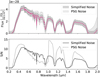 |
Fig. 1 Simulated observation of an Earth twin by the HWO concept assuming a simplified noise and a higher-fidelity noise instances. Top panel: the simulated observed flux at a distance of 10 pc between 0.2 and 2 μm for the two noise scenarios: simplified noise at constant error bars (shaded dark gray area with solid edges) and higher-fidelity simulated noise obtained with PSG (shaded light gray area with dotted edges). Bottom panel: signal-to-noise ratio (S/N) as a function of wavelength for the two noise instances: simplified noise (solid line) and PSG-simulated noise (dotted line). |
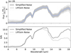 |
Fig. 2 Simulated observation of an Earth twin by the LIFE concept assuming a simplified noise and a higher-fidelity noise instances. Top panel: simulated observed flux at a distance of 10 pc between 4 and 18.5 μm for the two noise scenarios: simplified noise at constant error bars (shaded dark gray area with solid edges) and higher-fidelity simulated noise obtained with LIFESIM (shaded light gray area with dotted edges). Bottom panel: signal-to-noise ratio (S/N) as a function of wavelength for the two noise instances: simplified noise (solid line) and LIFESIM-simulated noise (dotted line). |
2.3 Updates on the Bayesian retrieval framework and setup
The Bayesian atmospheric retrieval framework used in previous studies (e.g., LIFE Papers III and V) has been updated to allow the correct simultaneous retrieval of both MIR and UV/VIS/NIR spectra. Generally, any Bayesian atmospheric retrieval framework is composed of two main modules: first, a parameter estimation module (pyMultiNest in this case, Buchner et al. 2014) to iteratively sample the prior space to retrieve the best subset of parameters that explains the data (the posteriors); and second, a forward model (petitRADTRANS in this case, Mollière et al. 2019) is used to calculate the spectrum corresponding to a set of parameters. The majority of the updates were performed to allow the use of features that were implemented in petitRADTRANS for LIFE Paper V (see Appendix A of Alei et al. 2022a) but that were not considered in the previous studies.
Firstly, we adapted the existing retrieval framework to handle multiple input spectra simultaneously to account for different resolutions, S/N, and wavelength ranges that are specific to the different instruments. We achieved this by calculating theoretical spectra at a resolution of R = 200, which is higher than the maximum foreseen resolution, and then binning these down to the input wavelength points at each retrieval iteration. For this step, we used the spectral rebinning tool SpectRes (Carnall 2017).
Secondly, we considered the atmospheric and surface scattering of both direct light and thermal atmospheric radiation as additional processes compared to previous studies. We assumed to know the stellar radius and temperature, incident angle, and the distance of the stellar-planet system fixed in the retrievals. We next introduced the surface reflectivity, rs, as a parameter to be retrieved in the various runs. In the case of a thin, cloud-free atmosphere, the surface reflectance makes up for the majority of the albedo of the planet. Therefore, having rs as a free parameter allows us to qualitatively analyze any degeneracy between albedo and radius at UV-VIS wavelengths (see, e.g., Gaudi et al. 2020; Feng et al. 2018). We refer to Appendix A for more details on the scattering treatment and the definition of the surface reflectance.
In the retrieval, we considered the same set of opacities that were used to calculate the input spectrum (see Table D.2). The retrieval framework also takes into account CIA and Rayleigh scattering (see Table D.3). This choice was made to minimize the biases that the use of different opacity line lists might cause. We refer to Alei et al. (2022b) for more details on such systematic errors.
The parameters considered in all retrievals and the assumed priors are described in Table D.1. Here, the priors are displayed as follows: 𝒰(x, y) represents a uniform (boxcar) prior with equal probability between a lower threshold, x, and an upper threshold, y; 𝒢(μ, σ) denotes a prior shaped like a Gaussian distribution with mean, μ, and standard deviation, σ). The priors are generally consistent with our previous studies (see LIFE Papers III and V), with differences in the assumed radius and mass priors. The radius prior is uniform between 0.5 and 2 R⊕, and the mass prior is a Gaussian with a mean of one and a standard deviation of 0.5 M⊕. These priors are wider than what we assumed in previous papers in the LIFE series. While LIFE will be able to gather narrower priors on the radius from the search campaign by measuring the emitted flux of the planet (see LIFE Paper II for details), the same assumptions could not be made in the case of reflected light measurements obtained with HWO. To allow both concepts to be comparable fairly, we selected larger priors that are realistic estimates of what could be a product of prior measurements that precede a prior detailed characterization campaign.
As in LIFE Papers III and V, in the retrieval we assumed the presence of a filling gas whose abundance is 1 − ∑(Xi), where Xi is the abundance of the chemical species included as free parameters (see Table D.1). The filling gas has a molecular weight of 28, assuming an N2-dominated mixture that is realistic for terrestrial planets. The filling gas only contributes to the mean molecular weight of the atmosphere and it is not spectroscopically active.
The retrieval also includes N2 as a free parameter to allow the inclusion of N2 Rayleigh scattering cross sections and N2-related CIA (see Table D.3). In principle, we could expect any gas (or mixture) of similar abundance and cross section to be able to model the same Rayleigh feature in the reflection spectrum. The use of N2 in our retrievals is to be interpreted as a representation of a noninteracting bulk Rayleigh scatterer with an average molecular weight of 28. To ensure this distinction is clear, we labeled this parameter in our plots as X2.
2.4 Methods for the significance analysis
Ultimately, when performing retrievals on either simulated or real data, we are interested in the significance of the detection of the main free parameters. In this work, we used established methodologies to quantify the significance of the detection of each atmospheric species with the single-instrument runs and the joint retrieval run.
2.4.1 Bayes factor
One well-known metric to quantify the robustness of a detection is the Bayes factor (see, e.g., Parviainen 2018, and references therein). The Bayes factor analysis allows us to compare two models to determine which one best reproduces the data with the smallest number of parameters. We can derive the Bayes factor by calculating the ratio of the Bayesian evidence, ![Mathematical equation: $\[\mathcal{Z}\]$](/articles/aa/full_html/2024/09/aa50320-24/aa50320-24-eq3.png) (D|ℳi), of two sets of models, given the data, D:
(D|ℳi), of two sets of models, given the data, D:
![Mathematical equation: $\[\mathcal{K}=\frac{\mathcal{Z}\left(\mathbf{D} \mid \mathcal{M}_1\right)}{\mathcal{Z}\left(\mathbf{D} \mid \mathcal{M}_2\right)}.\]$](/articles/aa/full_html/2024/09/aa50320-24/aa50320-24-eq4.png) (1)
(1)
By choosing as ℳ1 (ℳ2) a model that includes (excludes) a specific species in the atmosphere and comparing the Bayesian evidence, we can determine if the presence of that atmospheric species as a free parameter in the model is justified by the data. Jeffreys’ scale (Jeffreys 1998) allows us to then determine which model is preferred and with what confidence (see Table 1).
Jeffrey’s scale (Jeffreys 1998).
2.4.2 “Sigma” interpretation of the Bayes factor
Following Benneke & Seager (2013), we were also able to calibrate between Bayesian and frequentist detections by relating the value of 𝒦 to a level of significance. This conversion is possible provided the priors are either unimodal symmetric distributions or uniform, as it is in this study. In addition, the priors have to be the same for both models involved in the test. Then, the tests in the Bayesian and frequentist regimes become equivalent, since the priors cancel out (see Trotta 2017). However, the tests do not have the same meaning and interpretation due to the different frameworks. With the Bayesian interpretation, the posterior probability, P(ℳ1|D) gives probabilistic support that ℳ1 is more likely to be correct in comparison to ℳ2, provided that the two models exhaust the space of possible models. On the other hand, the frequentist P-value gives the probability of observing a test statistic value that is larger or equal to the one we observe, if the null hypothesis, ℋ0 (here associated with ℳ2), were to be correct. The P-value allows one to reject ℋ0 for a chosen type I error value. To ease up interpretation, the P-values are translated to a “sigma” value, as is frequently used in astronomy (see, e.g., Benneke & Seager 2013). This is to be interpreted as a complementary metric to the Bayes factor to determine the strength of the detection. In this case, only positive values are allowed, since no conclusive statement on the strength of the detection can be given when log10(𝒦) < 0 (i.e., when ℳ2, the model that excludes that species, is preferred). In Table 2, we show some relevant frequentist significance values and the corresponding Bayes factors and evidence strengths. We used these reference values to convert the 𝒦 values into “sigma.”
2.4.3 Mean-squared error
Since we are dealing with a simulated data scenario, we can exploit the knowledge of the true value to determine the precision and accuracy of the various retrievals. We used the mean-squared error, a metric that takes into account the variance of the posterior distribution and the distance of the mean of the posterior distribution from the true value. The mean-squared error of an “estimator” parameter, ![Mathematical equation: $\[\hat{\theta}\]$](/articles/aa/full_html/2024/09/aa50320-24/aa50320-24-eq9.png) , compared to the true parameter, θ, is defined as
, compared to the true parameter, θ, is defined as
![Mathematical equation: $\[\operatorname{MSE}(\hat{\theta})=\operatorname{Bias}(\theta, \hat{\theta})^2+\operatorname{Var}(\hat{\theta}),\]$](/articles/aa/full_html/2024/09/aa50320-24/aa50320-24-eq10.png) (2)
(2)
where Bias is the bias of the estimator, defined as the difference between the estimated value and the true value, and Var is the variance of the estimator. In our scenario, this translates into
![Mathematical equation: $\[\mathrm{MSE}=(\mu-\tau)^2+\sigma^2,\]$](/articles/aa/full_html/2024/09/aa50320-24/aa50320-24-eq13.png) (3)
(3)
where μ is the mean of the posterior distribution, τ is the true value, and σ is the standard deviation of the posterior distribution.
Since the priors assumed for various parameters span different ranges, we divided the posterior distribution of each parameter by the corresponding prior, so that the normalized posterior would become a value in the [0, 1] interval instead of the [x,y] interval. For the mass, whose prior was Gaussian, we assumed the edges of the prior to be 0 and the 5σ value from the mean of the Gaussian (3.5 M⊕). This allows us to represent all of the parameters with a single metric.
While this metric will not be available when dealing with real observations (since there will not be any true value to compare against), it can be useful at this stage of the development of the two future-generation concepts. By looking for the smallest MSE, we can identify the scenario that provides the most precise and accurate estimates of relevant parameters. To better appreciate such small variations, we used the square root of the mean squared error for our analyses. A similar metric to evaluate the performance of different retrieval runs has been used in other recent works such as Hayoz et al. (2023).
Translation table between some relevant frequentist significance values and their Bayesian interpretation, adapted from Benneke & Seager (2013) and Jeffreys (1998).
3 Results
We performed retrievals on the sets described in Sec. 2. Each set in turn contains three retrievals performed on either UV/VIS/NIR data (HWO-like), MIR data (LIFE-like), or joint retrievals on UV/VIS/NIR+MIR data (HWO+LIFE-like). These have been associated with the same colors throughout the manuscript (see Table 3 for details). We describe our results for the idealized high-resolution low-noise scenario (used for validation) in Appendix B. Here, we focus on the simplified noise scenario in Sec. 3.1, and the high-fidelity noise scenario in Sec. 3.2.
Details on the models run for each retrieval set and their color.
3.1 Simplified noise scenario
In this set of retrievals, we assumed the current baseline resolutions for LIFE and HWO. These are: R = 50 from 4 to 18.5μm for LIFE; R = 7 (0.2–0.5μm), R = 140 (0.515–1μm), and R = 70 (1.01–2μm) for HWO. For this set of retrievals, we kept a simplified noise instance (for more details see Sec. 2.2). In Figs. 3–5, we show a comparison of the retrieved spectra, the P-T profiles, and the posteriors for the three models in this set. The Bayes factors and confidence levels in σ values are shown in Fig. 6 and Table D.7. The values of the square root of the MSE are shown as bar plots in Fig. 7. The corner plot and a table containing the retrieved estimates with their 1σ uncertainty for each parameter can be found in Fig. D.1.
As is shown in Fig. 3, the retrieved spectrum is always within the noise uncertainty (shaded gray area) for all models. For the single-instrument retrievals, the retrieved spectra show larger uncertainties at short wavelengths where the noise is higher, as well as in some prominent lines. Such uncertainties on the retrieved spectrum are smaller in the HWO+LIFE retrieval, as we would expect from a retrieval performed on a larger amount of data which exploits a larger information content compared to the retrievals on a single wavelength range.
Regarding the characterization of the thermal structure of the atmosphere, the retrieval on LIFE data infers a more precise and accurate characterization of the atmosphere, though with increasing uncertainties toward lower pressures. This is related to the physics of the problem: as the majority of the radiation in the thermal emission spectrum comes from the deeper layers of the atmosphere and the surface, it is much easier to constrain the deeper layers of the atmosphere rather than the upper layers. The retrieved value of the ground pressure is around log10(P0) = −0.13, which corresponds to about 0.74 bar, with an uncertainty of ≈0.3 dex. The true surface pressure value is within an uncertainty of 1σ. The surface temperature is estimated as T0 = 284 ± 10 K, very close to the true value of 286 K.
The HWO run does not obtain the same accuracy on the thermal profile, with much wider uncertainties across all pressures. The ground pressure is overestimated as log10(P0) = 0.33 ± 0.25, which corresponds to ≈2.1 bar, a factor two larger than the expected value. The surface temperature is also much more loosely constrained at T0 = 335 ± 55 K, about 50 K hotter than the true value.
For the joint HWO+LIFE retrieval, the surface pressure is also slightly overestimated (retrieved log10(P0) = 0.27 ± 0.2, which corresponds to around 1.8 bar), though less than the HWO-only run.
The ground temperature retrieval obtained with a joint retrieval is more precise and accurate than any of the singleinstrument retrievals, with a retrieved ground temperature of T0 = 286 ± 6 K. The P-T profile is also retrieved correctly, with similar uncertainties as the LIFE retrieved profile (see Fig. 4) at lower pressures, but even smaller uncertainties in the deeper layers of the atmosphere.
When it comes to the characterization of the mass and radius, there is no substantial difference between the various runs (see Figs. 5 and D.1). The radius is accurately retrieved by all models with an uncertainty of 0.1 R⊕ or less. Specifically, the retrievals of LIFE and HWO are comparable with each other, while the HWO+LIFE one gets a more accurate constraint on the radius up to an uncertainty of 0.05 R⊕. The mass is consistently retrieved in all three retrievals, but its estimate is not significantly more precise than the input prior.
Regarding the reflectance, the HWO and HWO+LIFE retrievals correctly retrieve the value with comparable uncertainty, while LIFE alone does not manage to constrain this parameter. This shows that only the reflected-light portion of the spectrum contains enough information to correctly retrieve the reflectance of the planet, which was to be expected and which is confirmed by the idealized high-resolution low-noise scenario (see Appendix B).
By observing the posteriors in Fig. 5 we note that, generally, the posteriors of the joint retrievals are significantly smaller than the posteriors of the single models, especially when the LIFE and HWO retrievals are not consistently retrieving a parameter. The HWO+LIFE posteriors place themselves at the intersection of the posteriors of the single-instrument runs; this translates into smaller uncertainties on the estimates of most parameters and a greater decoupling of all correlated parameters. In other words, compared to single-instrument retrievals, a joint retrieval reduces the subset of possible parameters that can reproduce the data, particularly so when two or more parameters are correlated (e.g., the pressure and the main absorbing species of the atmosphere). This means that the joint retrieval correctly leverages the total amount of information available in the two wavelength ranges, as one would expect from the retrieval of complementary data.
Figures 5–7 quantify what we observed so far. The retrieval of the atmospheric species with LIFE is consistent with the previous papers in the series: LIFE can decisively constrain the abundance of H2O and CO2 (with more than 5σ confidence level), as well as strongly constrain O3 (3σ confidence). However, it is not sensitive to the bulk scatterer X2, O2, and CO, and can only retrieve upper limits on N2O and CH4. On the other hand, the HWO run poses strong constraints on O2 and H2O (5σ), while O3 is weakly constrained (at a <2σ confidence level). The other molecules (CH4, CO, CO2, N2O) are unconstrained or constrained with very broad upper limits. Through HWO retrievals, it is also possible to estimate the abundance of the bulk absorber X2 (see Sec. 4.1). The joint retrieval can retrieve with higher precision the species that were already retrieved in both the single-instrument retrievals. For all the molecules we retrieved, the HWO+LIFE retrieval obtains equal or higher confidence levels (Fig. 6) compared to the singleinstrument cases. Notably, it is possible to have a decisive detection of O3 compared to a weak and strong detection of the HWO and LIFE retrievals, respectively. This result is however dependent on the noise simulation, as will be seen in the next set of retrievals and further discussed in Sec. 4.3.
The mean-squared-error metric is also valuable to quantify the improvement of the joint retrieval compared to the singleinstrument scenarios (Fig. 7): for all the parameters considered in the retrieval, the estimate provided by the multi-instrument retrieval is comparable or significantly better in precision and accuracy compared to the single-instrument estimates (i.e., the value of ![Mathematical equation: $\[\sqrt{\mathrm{MSE}}\]$](/articles/aa/full_html/2024/09/aa50320-24/aa50320-24-eq16.png) of the HWO+LIFE retrieval for each parameter is the same or lower than the one from the single-instrument retrievals).
of the HWO+LIFE retrieval for each parameter is the same or lower than the one from the single-instrument retrievals).
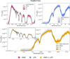 |
Fig. 3 Retrieved spectra for the “simplified noise” retrieval set. Left panel: pure HWO retrieval (magenta). Central panel: pure LIFE retrieval (blue). Right panel: HWO+LIFE retrieval (yellow). In all panels, the 2σ and the 1σ intervals are shown in increasingly darker hues, as well as the input spectra (black lines) with error bars (gray-shaded areas) for comparison. |
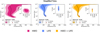 |
Fig. 4 Retrieved pressure-temperature profiles for the “simplified noise” retrieval set. Left panel: pure HWO retrieval (magenta). Central panel: pure LIFE retrieval (blue). Right panel: HWO+LIFE retrieval (yellow). In all panels, the 2σ and the 1σ intervals are shown in increasingly darker hues, as well as the input profiles (black lines) for comparison. Inside each panel, the inset plot shows the 2D posterior space of the ground pressure and temperature. In all panels and the inset plots, the surface pressure and temperature point in the P-T space is shown as a red square marker. |
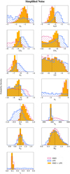 |
Fig. 5 Posterior density distributions from the “simplified noise” retrieval set. The black lines indicate the expected values for every parameter. HWO posteriors are shown in magenta with diagonal hatching. LIFE posteriors are shown in cyan with crossed hatching. HWO+LIFE posteriors are shown as fully colored yellow histograms. |
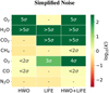 |
Fig. 6 Bayes factor and confidence levels values for each retrieved spectroscopically active species in the “simplified noise” retrieval set. The heatmap is color-coded according to the Bayes factor values log10(𝒦) and the confidence levels (in “sigma” values) are labeled within each cell whenever log10(𝒦) is positive. The Bayes factor values were obtained by performing a retrieval including and excluding the molecule of interest and then using Eq. (1). These were then converted into σ through Table 2. The Bayes factor values can be found in Table D.7. |
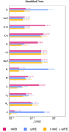 |
Fig. 7 Square root of the mean squared error (see Eq. (3)) for relevant parameters in the “simplified noise” retrieval set. |
3.2 Higher-fidelity Planetary Spectrum Generator and LIFE SIM simulated noise scenario
In this set of retrievals, we used the same “baseline” resolutions as the previous set but assumed a more complex noise instance, which was generated by the currently available noise simulators for the LIFE and the HWO concepts (as is described in Sec. 2.2). The results of this set of retrievals are shown in Figs. 8–10. The Bayes factor and confidence level values of the atmospheric species are shown in Fig. 11. The numeric values of the Bayes factor are reported in Table D.8. The square root of the mean squared error for the retrieved parameters is shown in Fig. 12. The corner plot and the retrieved estimates with their 1σ uncertainty for each parameter can be found in Fig. D.2.
The P-T profile is accurately retrieved with LIFE. On the other hand, the HWO run overestimates the ground pressure and temperature and constrains the atmospheric profile more loosely. The joint retrieval overestimates the ground pressure, but still retrieves a more accurate and precise estimate of the ground temperature compared to the single-instrument runs (T0 = 287 ± 6 K for the HWO+LIFE run compared to T0 = 336 ± 60 K for the HWO run and T0 = 285 ± 11 K for the LIFE run, compared to the true value of 286 K).
Regarding the atmospheric characterization (see Figs. 10–12) we observe some differences compared to the previous set of models. The retrieval on HWO data estimates with strong or decisive confidence (≥3σ confidence level) the abundances of O2, H2O, and O3. The confidence on the O3 detection is a definite improvement compared to the previous set, though at the expense of a lack of confidence in the retrieval of an upper limit of CO.
The performance of the LIFE retrieval does not significantly change in this scenario. Also for this set of retrievals, the joint retrieval of UV/VIS/NIR + MIR data produces results at least as confident as the single-instrument runs, estimating all free parameters with higher accuracy and precision compared to HWO- and LIFE-only retrievals (see Fig. 12). However, the joint retrieval is not able to confidently estimate CH4, CO, or N2O.
4 Discussion
In this section we discuss the results, focusing on the singleinstrument observations (Sec. 4.1), the joint observations (Sec. 4.2), and the impact of noise (Sec. 4.3). We discuss the limitations of our work in Sec. 4.4. To benchmark our results with the literature whenever possible, we compare the singleinstrument runs we performed in this work with other HWO-and LIFE-centered studies in Appendix C.
4.1 Strengths of single-instrument observations
In all the retrieval sets performed in this study, we can directly compare the potential of the two mission concepts in characterizing a Modern Earth-twin exoplanet. Most of the differences lie in the intrinsic planetary spectral features that are observable in different wavelength bands. Molecular oxygen has sharp features in the visible reflected-light spectrum, while ozone is prominent both in the UV (<0.3μm) and in the MIR (around 9.6μm). The CO2 band at 15μm is also a readily detectable feature, while H2O absorbs across most wavelengths. Because of these differences, we can retrieve with higher confidence specific molecules in the two wavelength ranges (see Figs. 5, 10, and B.3, as well as Tables D.7, D.8). In all baseline scenarios (simplified noise and high-fidelity noise), from the HWO retrievals we performed we can estimate O2, H2O, and O3; on the other hand, LIFE retrievals allow us to estimate CO2, H2O and O3. In both wavelength ranges, we also have upper limits on CH4 and N2O (see Figs. 5 and 10), though with very weak or no confidence for the baseline values. This is in agreement with what was found in the literature and our previous studies (see Appendix C). Importantly, even in the idealized scenario (photon noise only, R = 1000 and S/N = 50, see Appendix B), the single-instrument runs would still not be able to constrain CO and N2O for the HWO case, or O2 for the LIFE case (see Fig. B.5).
Observations in the UV/VIS/NIR are especially sensitive to the scattering processes (both Rayleigh and surface scattering), while MIR measurements would directly retrieve an estimate of the thermal structure of the atmosphere. These are results that can be observed clearly in all the runs (see, e.g., Figs. 5, 10, and B.3). Specifically, in the HWO retrievals the Rayleigh slope is well reproduced by the forward model (see, e.g., Figs. 3, 8, and B.1). The Rayleigh slope in the UV/VIS/NIR spectrum is mainly impacted by the most abundant molecules, which could be spectrally active (e.g., O2) or inactive (e.g., the bulk scatterer X2, which would correspond to N2 in an Earth-twin scenario). While the abundance of spectrally active species can be constrained through absorption lines in the spectrum, X2 can only be constrained through the modeling of the Rayleigh slope. With HWO-like observations, we would be able to infer the presence of a bulk scatterer X2, though further studies would be needed to properly assess the nature of the absorber itself (see Hall et al. 2023).
A correct retrieval of X2 and its contribution to scattering at short wavelengths in turn breaks the degeneracy between radius and reflectance: at short wavelengths, the planetary spectrum would become opaque because of Rayleigh scattering, so most of the incident flux never reaches the surface (see, e.g., Gaudi et al. 2020) – this allows these parameters to be retrieved with greater accuracy. On the other hand, retrievals of data at UV/VIS/NIR wavelengths cannot constrain the pressure-temperature profile to more than tens of degrees of uncertainty, even in the best-case scenario (see Fig. B.2). This result informs us that there is simply not enough information in the reflectedlight spectrum to accurately pinpoint the thermal profile of the atmosphere. At the baseline resolutions, HWO-like retrievals have the potential of also overestimating the ground pressure (see Figs. 4 and 9). This biased result is coupled with a lower estimate of the abundance of some molecules in the HWO-only runs (e.g., O2, H2O, O3), as a result of the well-known pressure-abundance degeneracy, observed in many previous studies (see Appendix C).
From the MIR point of view, strong absorption lines of CO2, H2O, and O3 allow one to precisely fit the P-T profile in the denser layer of the atmosphere (see, e.g., Figs. 4, 9, and B.2). LIFE retrievals fail to constrain the surface reflectance, rs. This was expected, since the stellar and thermal radiation that is scattered by the surface at MIR wavelengths is so little to be below the noise level. The only exception is the high-resolution case: the impact of the scattered light on the spectrum is greater than the noise level for surface reflectances higher than 0.3–0.4, which allows the retrieval framework to provide an upper limit on this parameter for MIR-only data. Still, other estimates of the albedo of the planet are accessible through LIFE-like retrievals. For example, from an accurate estimate of the radius, which LIFE would gather from the search campaign, it would be possible to get an estimate of the equilibrium temperature of the planet and, as a consequence, the Bond albedo of the planet (see, e.g., Konrad et al. 2023, i.e., LIFE Paper IX, for details).
When it comes to the interpretation of these results, single-instrument retrievals would allow us to gather plenty of information to characterize the atmosphere of a planet and its habitability. Retrievals performed considering only UV/VIS/NIR data would in principle allow us to determine that the planet has water vapor in the atmosphere, though the high uncertainty on the surface temperature and pressure would still make it unclear whether there could be liquid water on the surface. It would also be possible to detect oxygen, which is a key biosignature for Earth-like life, but the lack of accurate characterization of additional molecules such as CH4 and CO to constrain the redox state of the atmosphere would not necessarily rule out the abiotic false positive case, where oxygen is generated by non-biological processes such as photolysis (see, e.g., Domagal-Goldman et al. 2014; Meadows et al. 2018).
On the other hand, retrievals on MIR data (LIFE retrievals, in blue) could provide very strong constraints on CO2, H2O, and O3, which could in principle also point to the presence of a potentially inhabited planet. However, the relationship between O2 and its photo-chemical byproduct, O3, is not linear (see Segura et al. 2003; Kozakis et al. 2022). Also in this case, a low-quality estimate of CH4 might hinder the vetting of O2 in a potential abiotic scenario. Nevertheless, assuming higher baseline resolution and S/N levels for LIFE (see, e.g., LIFE Papers III and IX) would mitigate this problem by allowing a stronger constraint on the CH4 abundance. Earth-like abundances of N2O would also be not possible to detect at this resolution and noise level. A more accurate and precise characterization of the thermal profile of the atmosphere, possible through MIR retrievals, would provide more stringent results on the potential for liquid water on the surface, though no direct measurement of the surface reflectivity (and potential water and vegetation features) would be available.
These statements only apply in the case of modern Earth analogs, which are the focus of this study. Other scenarios might behave differently, depending on the atmospheric composition. An example is the Archean Earth scenario, when CO2 and CH4 were likely much more abundant in the atmosphere. The simultaneous detection of CO2 and CH4 is believed to be a signature of life on early Earth (Krissansen-Totton et al. 2018). The higher abundance of these two molecules in the early Earth would make the detection of these within reach of both HWO (see, e.g., Young et al. 2024a,b; Damiano & Hu 2022) and LIFE (see, e.g., Alei et al. 2022a, i.e., LIFE Paper V). Another example would be an atmosphere with enhanced biogenic N2O. Angerhausen et al. (2024, i.e., LIFE Paper XII) found that this molecule could be detectable with LIFE-like observations if present at plausible biological production fluxes.
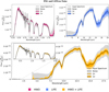 |
Fig. 8 Retrieved spectra for the “PSG and LIFESIM noise” retrieval set. Left panel: pure HWO retrieval (magenta). Central panel: pure LIFE retrieval (blue). Right panel: HWO+LIFE retrieval (yellow). In all panels, the 2σ and the 1σ intervals are shown in increasingly darker hues, as well as the input spectra (black lines) with error bars (gray-shaded areas) for comparison. |
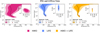 |
Fig. 9 Retrieved pressure-temperature profiles for the “PSG and LIFESIM noise” retrieval set. Left panel: pure HWO retrieval (magenta). Central panel: pure LIFE retrieval (blue). Right panel: HWO+LIFE retrieval (yellow). In all panels, the 2σ and the 1σ intervals are shown in increasingly darker hues, as well as the input profiles (black lines) for comparison. Inside each panel, the inset plot shows the 2D posterior space of the ground pressure and temperature. In all panels and the inset plots, the surface pressure and temperature point in the P-T space is shown as a red square marker. |
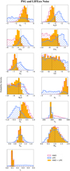 |
Fig. 10 Posterior density distributions from the “PSG and LIFESIM noise” retrieval set. The black lines indicate the expected values for every parameter. HWO posteriors are shown in magenta with diagonal hatching. LIFE posteriors are shown in cyan with crossed hatching. HWO+LIFE posteriors are shown as fully colored yellow histograms. |
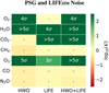 |
Fig. 11 Bayes factor and confidence levels values for each retrieved spectroscopically active species in the “PSG and LIFESIM noise” retrieval set. The heatmap is color-coded according to the Bayes factor values, log10(𝒦), and the confidence levels (in “sigma” values) are labeled within each cell whenever log10(𝒦) is positive. The Bayes factor values were obtained by performing a retrieval including and excluding the molecule of interest and then using Eq. (1). These were then converted into σ through Table 2. The Bayes factor values can be found in Table D.8. |
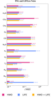 |
Fig. 12 Square root of the mean squared error (see Eq. (3)) for relevant parameters in the “PSG and LIFESIM noise” retrieval set. |
4.2 Complementarity of multi-instrument observations
From what we have seen in this study, multi-instrument observations are clearly helpful for reducing biases and overall enhancing the quality of the results. For each set, the posterior distributions of the joint retrieval run are mostly at the intersection of the single-instrument results (see the corner plots in Figs. B.5, D.1, and D.2). The posteriors also show a reduced bias and a smaller variance around the true value (see the mean-squared-error bar plots in Figs. 7, 12, and B.4).
Having data spanning a larger wavelength range translates into an increase in the number of spectral features to compare the forward model against when performing a Bayesian retrieval. It further becomes easier to disentangle overlapping features, by including more bands where each specific molecule can be more unambiguously detected. This limits the range of parameter space that can accurately reproduce the data, shrinking uncertainties (see Figs. 5, 12, and B.3). From the point of view of the atmospheric structure, different wavelength bandpasses sample different pressures throughout the atmosphere, allowing us to have a more precise thermal structure when including data from HWO and from LIFE, compared to the single-instrument counterparts (see Figs. 4, 9, and B.2).
At the baseline resolution values (simplified noise and high-fidelity noise scenarios) a joint HWO+LIFE retrieval on a cloud-free Earth-like planet would yield very strong constraints on O2, O3, CO2, and H2O, as well as weak constraints on CH4 and CO. In our runs, the confidence level for the detection of each of the considered species in the joint retrieval scenario is at least equal to the larger one between the two single-instrument retrievals and it increases considerably in some cases (e.g., O3, see Figs. 7 and 12). This shows that, whenever enough information is stored in one portion of the wavelength spectrum, this is also similarly detected with a joint retrieval. If, however, both portions of the spectrum contain information on a specific parameter, then the joint retrieval performance is magnified.
The joint retrievals also slightly overestimate the ground pressure. This is probably due to the UV/VIS/NIR spectrum which, as we have discussed in the previous subsection, is not sensitive to the atmospheric thermal profile but that has a marginally higher resolution than the MIR thermal emission spectrum. Therefore, the forward model might favor the strong O2 lines in the reflected spectrum, which tend to skew the result toward high pressures and low abundances, as it happens in the HWO-only retrievals. The overestimation of the ground pressure would in principle slightly increase the range of temperatures at which water can be liquid. However, the precise and accurate estimate of the surface temperature (retrieved with an uncertainty of ≈5 K when considering joint retrievals) would be more convincing about the habitability of a promising target, compared to the single-instrument runs.
A joint retrieval would therefore provide the highest quality of information available for a target. While an increase in the quality of the results compared to the single-instrument retrievals may seem quite obvious since the joint retrieval can leverage all the available information throughout the wavelength range, this represents a strong validation of our base assumption that the sum of both missions would be greater than each separately. This set of runs also serves as a “proof of concept” for a joint characterization of a terrestrial planet since it highlights how transformational the multi-wavelength observation of a promising planet could be, especially when trying to characterize the habitability of a potential candidate host for life.
Furthermore, a detailed characterization of both the reflected and the thermal portions of the planetary spectrum would help break the radius-albedo ambiguity by enabling an energy-budget analysis of the planet. By constraining both the albedo and the abundance of various greenhouse gases, it would be possible to estimate the expected greenhouse effect given the observed surface temperature and atmospheric profile, which would be a prerequisite for an accurate assessment of the habitability of the planet. Estimating the surface temperature with high precision would also refine the search for life by determining the likelihood of the presence of surface water; this would be a key piece of information needed to identify a promising target for further in-depth study, and it would likely not be prior available information.
Finally, the population-level results will be much more robust with both reflected light and thermal emission. Observations in both wavelength ranges will help us characterize the diversity of the planetary atmospheres that both missions will observe, paving the way for an unbiased, complete picture of the demographics of the sample.
4.3 Impact of noise
At this stage, accurate noise models that are specific to the two concepts are not yet fully developed. The development of these tools is strongly coupled with the architecture trades and the technological assessments that are currently in progress and will be executed over the coming years. However, it is assumed that we will be dealing with very small signals. In this “low-quality” data regime, different noise instances might be the reason for the detection or non-detection of specific molecules.
In this study, we used various noise instances to explore the impact that noise has in the retrievals. As is explained in Sec. 2.1, the noise level was the only difference between the “simplified noise” and “PSG and LIFESIM noise” retrievals. By comparing these sets of retrievals (see Sec. 3) we find that a more complex noise modeling causes some differences in the results. The most noticeable one is the detection of O3, which can be decisively detected thanks to the lower noise level in the UV band in the high-fidelity noise set compared to the very weak confidence in the detection in the simplified noise set. This highlights the great impact that accurate noise modeling could have in defining the requirements of future-generation missions and in prioritizing some architectures compared to others. As we progress in the definition of the various concepts, the noise models will need to be updated and these results will likely change. It is therefore important at this stage of the concepts’ maturation to benchmark results and to simulate observations through atmospheric retrievals, since these will provide information that will be fed back into the definition of the preferred architectures.
4.4 Known limitations of this study
The results discussed in this work are valid within the assumptions that were made. To simplify the problem and to provide a first-order overview, we used a simplified, cloud-free scenario that is not purely motivated by physics and is unlikely to be found in reality. In this scenario, it is possible to disentangle the correlation between the radius and the albedo through a high-resolution characterization of the Rayleigh cross section in the UV/VIS/NIR. However, this would most likely not be the case when clouds and hazes are present (see, e.g., Feng et al. 2018; Robinson & Salvador 2023; Damiano & Hu 2022). A MIR observation should be less prone to such issues (see LIFE Paper IX).
Furthermore, we used a simplified retrieval framework to allow for reasonable computing time (see Sec. 2.3 for details). Some further biases in the detection of the most abundant species in the atmosphere (the bulk scatterer X2 and O2) could have been caused by pyMultiNest, since this nested sampling algorithm has been found to undersample the edges of the prior space (see Appendix D of Himes 2022), which is the case for these two molecules. This bias could have especially negatively influenced the retrievals in the UV/VIS/NIR range, for which it was possible to constrain such molecules. Retrievals on the MIR portion of the spectrum would not have suffered from this bias, since not enough information about these molecules is contained in this range.
We assumed that we would perfectly know the geometry of the planet-star system, set at quadrature, and that the planet signal was fixed: rotation and atmospheric dynamics that happen on daily or seasonal timescales could be ignored. In reality, the phase of the system is likely to be unknown in this kind of observation and will need to be accurately modeled in retrievals.
Finally, we did not randomize the individual spectral points according to the noise, but rather we considered the noise as an uncertainty to the theoretically simulated flux points. This has been done in previous studies (see Appendix C), but it could lead to an overestimation of the results. In the Appendix of LIFE Paper III we compared the results of retrievals on non-randomized and randomized flux points, showing that results on non-randomized spectra could be interpreted as average estimates of the randomized-spectra results.
These issues will be overcome and improved in future studies. Some other limitations are however much more rooted in the development of these concepts themselves and the technical challenges that stem from that.
First of all, the noise treatment should be improved and updated as long as the iterations for various architecture trades proceed. Given the impact that noise could have on the confidence of the detection of important life-related molecules (as is shown by comparing the two baseline sets of retrievals), it is mandatory to keep refining the instrumental parameters that have an impact on the noise. This will also help define the observing time required for each observation to achieve the desired S/N. Once we get a better understanding of the processes that cause the spectral shape of the noise to change with exposure time, it will be possible to simulate accurate noise instances at the required observing time, instead of scaling a template noise to the desired S/N as it was done in this study. Retrieval benchmark studies will then need to be repeated to identify the architecture that yields the best possible results.
HWO will very likely include a coronagraph. This will require the presence of specific, multiple spectral bandpasses in the three wavelength ranges. We would not necessarily expect to have access to a complete spectrum of the planet in the UV/VIS/NIR range, like it was assumed here. Although some initial studies on the observation strategy (Young et al. 2023) and on how these bandpasses should be defined for HWO (Latouf et al. 2023a,b) were performed, these are still to be confirmed. Since acquisitions in the same wavelength range are limited to one bandpass at a time (Young et al. 2023) and since we would deal with long exposure times (of the order of hours, or even days), it is likely that the geometry of the planet-star system would change between one acquisition and another. This would complicate the modeling and the retrieval of realistic results.
We used a relatively large prior on the radius to allow for comparable retrieval results for both wavelength ranges of interest. However, a LIFE-like mission should be able to provide more stringent constraints on the radius from the search campaign (see LIFE Paper II) which could be used as prior for retrievals in both wavelength ranges and therefore potentially allow a more accurate retrieval of the planetary radius. Similarly, we could imagine that an improvement in the prior estimate of the mass (e.g., leveraging prior observations and/or the search campaign of a MIR LIFE-like mission) would improve the results.
At this stage, it is entirely plausible that the two missions will not fly at the same time, but rather one before the other. The added complexity of multi-epoch observations might bring its own set of challenges, as the geometry of the observation has likely changed and phase modeling will need to be taken into account. In the context of finding more robust clues for the presence of life on an exoplanet, joint retrievals on UV/VIS/NIR+MIR data might not be the best strategy, as one would have to merge data at different ephemerids. It might be more efficient to use the posteriors of a retrieval performed on data from one mission as priors for retrievals performed in the other spectral range. However, as we have seen in this study, biases are present in single-instrument retrievals. Therefore, it would be more realistic to select only the results we are more confident in to feed into future retrievals. For example, one should be more confident in the radius estimate given by retrievals in the MIR, rather than the UV/VIS/NIR. Similarly, the detection of O2 through UV/VIS/NIR could be fed into retrievals on MIR data to improve the determination of the molecular weight of the atmosphere. Given the strong complementarity of these results, such strategies might play a role in maximizing the yield from these missions. Further studies are required to assess which parameters are more likely to be constrained by which concept (and wavelength range) over a variety of case scenarios that go beyond a cloud-free Earth twin.
5 Conclusions
In this study, we performed atmospheric Bayesian retrievals on simulated data from an HWO-like mission and a LIFE-like one to assess the science potential of the two concepts separately and in synergy with each other for the characterization of a simplified Earth twin. To do this, we produced simulated observations of a cloud-free terrestrial planet both in reflected light and thermal emission. Furthermore, the retrieval routine that we developed for previous LIFE-related studies (e.g., Konrad et al. 2022; Alei et al. 2022a; Konrad et al. 2023; Mettler et al. 2024) has been updated to consider both UV/VIS/NIR and MIR spectra.
We considered two scenarios: a simplified noise model at constant error bars considering the baseline resolutions for the various wavelength ranges of interest, and a more complicated noise model using the current noise simulators available for LIFE and “6-m LUVOIR-B” as a template for HWO.
We conclude that:
Retrievals considering purely data from one of the two instruments would not provide a full characterization of the atmosphere and thermal structure of the planet. A retrieval on UV/VIS/NIR data alone strongly constrains O2 and H2O, and retrieves an upper limit on CH4. A retrieval on MIR data strongly constrains CO2, H2O, and O3, and also an upper limit on CH4. Neither of the two concepts can sufficiently constrain Earth-like abundances of CO and N2O, which are both relevant, to rule out abiotic processes (for the former) and assess metabolic activity (for the latter) (see, e.g., Schwieterman et al. 2018). LIFE retrievals would constrain the thermal profile of the atmosphere, while HWO retrievals would allow one to constrain the surface reflectance (in the absence of clouds).
Independent of the noise and the spectral resolution, a joint UV/VIS/NIR+MIR retrieval can improve the confidence level of the detection of the main potential biosignatures and bioindicators. Retrievals on UV/VIS/NIR+MIR constrain all the species that the single-instrument runs estimate, but increase the confidence of the estimates themselves: O2, CO2, H2O, and O3 would be detected with decisive confidence, while CO and CH4 could be weakly detected. Joint retrievals also improve the estimation of the surface temperature and pressure, as well as the radius.
Different noise assumptions can critically impact the results: the most realistic noise scenario (PSG and LIFESIM noise) would allow one to strongly retrieve O3 on UV/VIS/NIR -only data, while it would be only possible to get a low-significance constraint on that species in the simplified noise case. This result suggests that a higher-fidelity noise model could allow more accurate results that could drive the definition of the requirements of these missions. Further, the spectral resolution and S/N reference values are still up for discussion and in this work we only explored a small section of the R-S/N parameter space. The refinement of science requirements will be an iterative process that will continue over time as technological progress is made and as noise simulators take more and more realistic instrumental processes into account.
This has been the first study on the possible synergies between HWO and LIFE in characterizing habitable exoplanets, in support of the development of both by the community. Both wavelength ranges provide us with a specific set of unique information and come with specific drawbacks. Yet, the scientific yield of synergistic observations in the UV/VIS/NIR+MIR range has the potential to be greater than the sum of its parts. Having access to multiple spectral windows onto the atmosphere of a potentially habitable planet could be transformative for the search for life in the Universe.
Acknowledgements
E.A. work has been partly carried out within the framework of the NCCR PlanetS supported by the Swiss National Science Foundation under grants 51NF40_182901 and 51NF40_205606. E.A. research was partly supported by an appointment to the NASA Postdoctoral Program at the NASA Goddard Space Research, administered by Oak Ridge Associated Universities under contract with NASA. S.P.Q. work has been carried out within the framework of the NCCR PlanetS supported by the Swiss National Science Foundation under grants 51NF40_182901 and 51NF40_205606. E.O.G gratefully acknowledges the financial support from the Swiss National Science Foundation (SNSF) under project grant number 200020_200399. V.K. is supported by the GSFC Sellers Exoplanet Environments Collaboration (SEEC) and the Exoplanets Spectroscopy Technologies (ExoSpec). P.M. acknowledges support from the European Research Council under the European Union’s Horizon 2020 research and innovation program under grant agreement No. 832428. E.A. acknowledges T. Birbacher, F. Dannert, S. Gaudi, S. Mahadevan, B. Mennesson, A. Roberge, G. Villanueva, and A. Young for their expertise and useful discussions. We thank an anonymous reviewer for the helpful comments. CRediT author statement. E.A.: Conceptualization, Methodology, Software, Validation, Formal Analysis, Investigation, Data Curation, Writing - Original Draft, Visualization; S. P. Quanz: Conceptualization, Resources, Writing – Review and Editing, Supervision, Project Administration, Funding Acquisition; B. S. Konrad: Methodology, Software, Writing – Review and Editing; E. Garvin: Formal Analysis, Writing – Review and Editing; V. Kofman: Methodology, Writing – Review and Editing; A. Mandell: Methodology, Writing – Review and Editing; D. Angerhausen: Writing – Review and Editing; P. Mollière: Writing – Review and Editing; M. Meyer: Writing – Review and Editing; T. Robinson: Writing – Review and Editing; S. Rugheimer: Writing – Review and Editing. Software. This research made use of: Astropy2, a community-developed core Python package for Astronomy (Astropy Collaboration 2013, 2018); Matplotlib3 (Hunter 2007); pandas (Pandas development team 2020); petitRADTRANS (Mollière et al. 2019); PSG (Villanueva et al. 2022).
Appendix A Scattering of terrestrial exoplanets in reflected light
petitRADTRANS (Mollière et al. 2019) performs radiative transfer calculations including scattering through the Feautrier method (Feautrier 1964). We used the Feautrier method in LIFE Paper V only considering the thermal planetary radiation and we refer to Appendix A of LIFE Paper V for details on the implementation of that process, as well as Mollière (2017). Here, we report the main equations and we discuss the additional terms that are now taken into account to calculate the scattering by direct stellar light.
The radiative transfer equation (see Eq. A.1) depends linearly on the intensity, so planetary and stellar radiation fields can be treated in an additive way.
![Mathematical equation: $\[\mu \frac{d I}{d \tau}=-I+S.\]$](/articles/aa/full_html/2024/09/aa50320-24/aa50320-24-eq19.png) (A.1)
(A.1)
In this equation, μ = cos θ where θ is the angle between a light ray and the surface normal, τ is the optical depth, I is the intensity, and S is the source function.
In the Feautrier algorithm, the intensity vectors parallel and anti-parallel to the direction of a light ray (I+ and I−, respectively) are defined. The radiative transfer equation is then solved for the sum and the difference of these two rays (see LIFE Paper V). Two boundary conditions need to be defined at the top of the atmosphere (TOA; corresponding to P = 0) and at the surface (P = Ps). In the case of planetary radiation scattering only (used in LIFE Paper V), the conditions are:
![Mathematical equation: $\[I_{+}(P=0, \mu)=0 \quad \forall \mu\]$](/articles/aa/full_html/2024/09/aa50320-24/aa50320-24-eq20.png) (A.2)
(A.2)
![Mathematical equation: $\[I_{-}\left(P=P_s, \mu\right)=e_s B\left(T_s\right)+r_s J^{s c a t}\left(P_s\right).\]$](/articles/aa/full_html/2024/09/aa50320-24/aa50320-24-eq21.png) (A.3)
(A.3)
Where es is the surface emissivity; rs is the surface reflectance; B(Ts) is the blackbody emission of the surface; and Jscat the average scattered intensity of the radiation that comes from the top layers. The interpretation of these conditions is that: (1) there is no planetary radiation coming from the top of the atmosphere and (2) the light going upward from the surface is composed by the thermal emission of the surface itself (as the blackbody radiation of the surface scaled by the surface emissivity) and by a portion of the incoming planetary radiation that is reflected by the surface (as the average scattered intensity of the radiation that comes from the top layers scaled by the surface reflectance). Jscat is calculated as follows:
![Mathematical equation: $\[J^{s c a t}\left(P_s\right)=\int_0^1 I_{+}\left(P_s\right) d \mu\]$](/articles/aa/full_html/2024/09/aa50320-24/aa50320-24-eq22.png) (A.4)
(A.4)
In the case of scattering of stellar radiation, it is possible to split the incoming stellar intensity into two components: the incoming stellar radiation ![Mathematical equation: $\[I_*^{d i r}\]$](/articles/aa/full_html/2024/09/aa50320-24/aa50320-24-eq23.png) along the TOA incidence angle that survives down to a given layer of interest and which gets attenuated through absorption and scattering, and the stellar light that is scattered (potentially multiple times) in the atmosphere
along the TOA incidence angle that survives down to a given layer of interest and which gets attenuated through absorption and scattering, and the stellar light that is scattered (potentially multiple times) in the atmosphere ![Mathematical equation: $\[I_*^{{scat }}\]$](/articles/aa/full_html/2024/09/aa50320-24/aa50320-24-eq24.png) .
.
![Mathematical equation: $\[I_*=I_*^{d i r}+I_*^{{scat }}\]$](/articles/aa/full_html/2024/09/aa50320-24/aa50320-24-eq25.png) (A.5)
(A.5)
The radiative transfer equation for these components becomes (ϵ being the photon destruction probability):
![Mathematical equation: $\[\frac{d I_*^{d i r}}{d \tau}+\frac{d I_*^{s c a t}}{d \tau}=-I_*^{d i r}-I_*^{s c a t}+(1-\epsilon)\left(J_*^{d i r}+J_*^{s c a t}\right)\]$](/articles/aa/full_html/2024/09/aa50320-24/aa50320-24-eq26.png) (A.6)
(A.6)
Which can be split into two equations:
![Mathematical equation: $\[\frac{d I_*^{d i r}}{d \tau}=-I_*^{d i r}\]$](/articles/aa/full_html/2024/09/aa50320-24/aa50320-24-eq27.png) (A.7)
(A.7)
![Mathematical equation: $\[\frac{d I_*^{s c a t}}{d \tau}=-I_*^{s c a t}+(1-\epsilon)\left(J_*^{d i r}+J_*^{s c a t}\right)\]$](/articles/aa/full_html/2024/09/aa50320-24/aa50320-24-eq28.png) (A.8)
(A.8)
Equation A.7 is the regular attenuation of the direct light while crossing the atmosphere. Its solution is:
![Mathematical equation: $\[I_*^{d i r}=I_*^{d i r}(0, \mu) e^{-\tau / \mu}\]$](/articles/aa/full_html/2024/09/aa50320-24/aa50320-24-eq29.png) (A.9)
(A.9)
Where ![Mathematical equation: $\[I_*^{d i r}(0, \mu)\]$](/articles/aa/full_html/2024/09/aa50320-24/aa50320-24-eq30.png) is the irradiation at the TOA.
is the irradiation at the TOA.
For Eq. A.8, the calculation of ![Mathematical equation: $\[J_*^{d i r}\]$](/articles/aa/full_html/2024/09/aa50320-24/aa50320-24-eq31.png) is dependent on the geometry of the problem.
is dependent on the geometry of the problem.
In the case of isotropic stellar irradiation, ![Mathematical equation: $\[I_*^{d i r}(0, \mu)\]$](/articles/aa/full_html/2024/09/aa50320-24/aa50320-24-eq32.png) is integrated over all possible angles (−90° to +90° angle between the ray and the direction normal to the surface, which corresponds to the light that comes from the top). This translates as:
is integrated over all possible angles (−90° to +90° angle between the ray and the direction normal to the surface, which corresponds to the light that comes from the top). This translates as:
![Mathematical equation: $\[I_*^{d i r}(0)= \begin{cases}F_*^{d i r}(0) / \pi, & \text { if } \mu<0 \\ 0, & \text { otherwise }\end{cases}\]$](/articles/aa/full_html/2024/09/aa50320-24/aa50320-24-eq33.png) (A.10)
(A.10)
Where ![Mathematical equation: $\[F_*^{d i r}(0)\]$](/articles/aa/full_html/2024/09/aa50320-24/aa50320-24-eq34.png) is the stellar flux scaled at the distance of the planet. The average direct intensity over all angles is then:
is the stellar flux scaled at the distance of the planet. The average direct intensity over all angles is then:
![Mathematical equation: $\[J_*^{d i r}=\frac{1}{2} \int_{-1}^1 I_*^{d i r} d \mu=\int_0^1 I_*^{d i r} d \mu\]$](/articles/aa/full_html/2024/09/aa50320-24/aa50320-24-eq35.png) (A.11)
(A.11)
For non-isotropic irradiation (i.e., the stellar irradiation is incident under an angle θ* of cosine μ*), the value of ![Mathematical equation: $\[F_*^{d i r}(0)\]$](/articles/aa/full_html/2024/09/aa50320-24/aa50320-24-eq36.png) is:
is:
![Mathematical equation: $\[F_*^{d i r}(0)=\int_{\Delta \Omega_*} I_*^{d i r} \mu d \Omega \approx I_*^{d i r}(0) \mu_* \Delta \Omega_*\]$](/articles/aa/full_html/2024/09/aa50320-24/aa50320-24-eq37.png) (A.12)
(A.12)
Where ΔΩ* is the solid angle subtended by the stellar disk from the atmospheric location. In this case, ![Mathematical equation: $\[J_*^{d i r}\]$](/articles/aa/full_html/2024/09/aa50320-24/aa50320-24-eq38.png) is:
is:
![Mathematical equation: $\[J_*^{d i r}=\frac{I_*^{d i r} \Delta \Omega_*}{4 \pi}=\frac{F_*^{d i r}(0) e^{-\tau / \mu_*} \Delta \Omega_*}{4 \pi \mu_*}\]$](/articles/aa/full_html/2024/09/aa50320-24/aa50320-24-eq39.png) (A.13)
(A.13)
The stellar light that can be scattered at the surface is then calculated analogously to Eq. A.4 for the stellar radiation field and added to the planetary radiation field. Jscat will now automatically include both contributions from the atmospheric thermal radiation, and the stellar one, scattered at least once inside the atmosphere.
To meet the boundary condition, the mean direct radiation must be included in the term that takes into account the portion of radiation reflected by the surface. Therefore, Equation A.3 becomes
![Mathematical equation: $\[I_{-}\left(P_{{surf }}\right)=e_s ~B\left(T_{{surf }}\right)+r_s\left[J^{{scat }}\left(P_{{surf }}\right)+J_*^{{dir }}\left(P_{{surf }}\right)\right]\]$](/articles/aa/full_html/2024/09/aa50320-24/aa50320-24-eq40.png) (A.14)
(A.14)
In our study, we simulated the quadrature phase of the planet by assuming a non-isotropic scenario with a specific angle θ* = 77.756 degrees. In principle, every region of the planet would have a specific angle of incidence of the stellar light, so we should take into account the reflected spectrum of each pixel encompassed by the field of view. In the case of a Lambertian surface, which is what we assumed in this study, this calculation can be simplified by averaging the angles across the field of view. This produces an “average” incident direct light angle of 77.756 degrees, which allowed us to run a single radiative transfer simulation with reasonable results. For more information on this treatment, used widely in the Planet Spectrum Generator suite, we refer to the PSG Handbook (Villanueva et al. 2022).
The surface reflectance rs assumed in the scattering calculation is a free parameter in our runs. It represents the specific reflectance of the surface material. In principle, petitRADTRANS can assume a wavelength-dependent reflectance of a custom surface. The user can take advantage of known reflectivity databases (e.g., the United States Geological Survey Spectral Library, Kokaly et al. 2017) to fill this variable. In this study, we assumed a wavelength-independent value of rs of 0.1 (an average value for habitable water-rich terrestrial planets) both when producing the input spectrum and when retrieving the rs estimate.
The value of rs was therefore different from what is commonly assumed to be the albedo of the planet as a whole, as no contribution from the atmosphere was considered aside from the extinction of the incoming ray that is reflected by the surface. However, in the case of thin enough atmospheres with no clouds such as the one considered in this study, the majority of the scattered light that would be detected originates from the surface. For this reason, in this specific case, rs can be considered a proxy for planetary albedo. The Bond albedo of the planet a posteriori can be retrieved from the planetary radius estimate and the stellar luminosity, as it was done in Konrad et al. (2023); Mettler et al. (2024).
Appendix B Idealized high-resolution low-noise scenario
In this set of runs, we simulated the spectrum of a cloud-free Earth at R = 1000 with uncertainties based on a S/N = 50 at 0.55μm and 11.2μm, only taking photon noise into account. This serves as a validation of the updated retrieval routine and represents an idealistic best-case scenario. In Figs. B.1, B.2, and B.3, we show the best fit of the spectrum compared to the input data, the retrieved P-T profiles, and the posteriors of the main physical and chemical parameters for this retrieval set. The corresponding corner plot is shown as Fig. B.5. The square root of the mean squared error for various parameters is shown in Fig. B.4.
As can be noticed in Fig. B.1, we are able to accurately and precisely reproduce the input spectra in all the scenarios. The 1-, 2-, and 3σ envelopes of the retrieved spectrum lie well within the photon noise uncertainty. For better clarity of this set of plots, we do not show the σ envelopes for the best-retrieved spectra in this case, but only the best fit.
Retrieving an accurate P-T profile is satisfactory with LIFE: the profile is correctly determined down to pressures of approximately 10−3 bar. This is expected, since for a cloud-free thin-atmosphere scenario the majority of the contribution to the thermal emission spectrum is coming from the lower, denser layers of the atmosphere. In the LIFE retrieval, the surface pressure and temperature are also retrieved with high precision and accuracy (with a 1 σ uncertainty of 0.06 dex for the pressure, and only 0.5 K for the temperature). The HWO retrieval is less accurate, as can be seen from the larger envelopes in the P-T profile. The retrieval of surface temperature and pressure is relatively accurate (the 1σ interval uncertainty of T0 is around 15 K in this case). The joint retrieval can estimate the P-T profile with better accuracy and precision than the single-instrument retrievals. Fig. B.3 shows that, in the case of the idealized HWO+LIFE retrieval, the uncertainties on the surface pressure and temperature are reduced (up to a 1σ uncertainty of 0.03 dex for P0 and 0.3 K for T0). This result stems from the high quality of the spectrum, which allows the retrieval framework to correctly model pressure and thermal broadening of each line – and especially the deeper layers of the atmosphere that contribute the most to the spectrum.
The retrieval of the radius is very accurate and precise in all three retrievals: the estimate of the radius and corresponding 1σ uncertainty is 1 ± 0.01 R⊕ or lower for all scenarios. Retrievals that include MIR data (LIFE and HWO+LIFE retrievals) can leverage the thermal emission of the planet, which provides a strong constraint on the radius of the planet (see, e.g., LIFE Paper III). On the other hand, the result of the HWO retrieval is dependent on the assumptions made in this study. Since we neglect clouds and assume a perfect knowledge of the geometry of the system, the radius/albedo degeneracy in the UV/VIS/NIR can be easily disentangled. This will likely not be the case in reality, as is discussed in Sec. 4.4.
Concerning the planetary mass, even the most idealized scenario of a MIR LIFE-like retrieval only slightly further constrains the mass of the planet compared to the prior (retrieving a mass of Mp1 = 1.08 ± 0.30 M⊕). This happens because of the well-known degeneracy between gravity and chemical abundances, which contribute to the scale height of the atmosphere (see LIFE Papers III and V for details). On the other hand, the UV/VIS/NIR retrieval allows for a more precise estimate of the mass with an uncertainty of about 10%, but a less accurate result (estimating Mp1 = 0.88 ± 0.10 M⊕). Considering both wavelength ranges together would instead improve the mass estimate to Mp1 = 0.94 ± 0.07 M⊕, with the true value within the 1σ confidence interval.
The surface reflectance is accurately and precisely determined by the HWO retrieval. On the other hand, the LIFE retrieval can only rule out surface reflectances higher than 0.3–0.4. Further, there are slight correlations between rs and the major atmospheric absorbers in the MIR. The combined HWO+LIFE retrieval retrieved this parameter correctly. The surface reflectance is also impacted, like the radius, by the assumptions we make in these studies regarding geometry and clouds (see Sec. 4.4).
At such high spectral resolution and S/N, the retrievals are generally precise and accurate at retrieving the abundances of the main atmospheric species. There are, however, a few exceptions. Even in the most idealized HWO retrieval, it is not possible to have a detection of CO and N2O (only upper limits are retrieved). These two molecules do not have significant lines in this wavelength range (the opacity being 3–4 orders of magnitude fainter than the main absorbers in this range, such as O2 and H2O). In the idealized LIFE retrieval, O2 cannot be sufficiently constrained, because of the lack of significant lines in the MIR wavelength range. CO has a strong detection peak around the true value, but lower abundances cannot be entirely ruled out. This is due to its main spectral features being at short MIR wavelengths (≤4.5μm), where the noise is large due to the lower thermal emission of the planet. These spectral lines also overlap with features of more abundant species (mainly H2O, CO2, and O3) which makes the less abundant species harder to detect.
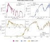 |
Fig. B.1 Best-fit spectra retrieved in the “idealized high-resolution low-noise” retrieval set (photon noise only at S/N = 50, R = 1000) for the three scenarios. Left panel: Pure HWO retrieval (magenta). Central panel: Pure LIFE retrieval (blue). Right panel: HWO+LIFE retrieval (yellow). In all panels, the best-fit spectra are compared with the input spectra (black lines) with error bars (gray-shaded areas). |
 |
Fig. B.2 Retrieved pressure-temperature profiles for the “idealized high-resolution low-noise” retrieval set (photon noise only at S/N = 50, R = 1000). Left panel: Pure HWO retrieval (magenta). Central panel: Pure LIFE retrieval (blue). Right panel: HWO+LIFE retrieval (yellow). In all panels, the 2σ and the 1σ intervals are shown in increasingly darker hues, as well as the input profiles (black lines) for comparison. Inside each panel, the inset plot shows the 2D posterior space of the ground pressure and temperature. In all panels and the inset plots, the surface pressure and temperature point in the P-T space is shown as a red square marker. |
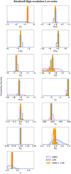 |
Fig. B.3 Posterior density distributions from the “idealized highresolution low-noise” retrieval set (photon noise only at S/N = 50, R = 1000). The black lines indicate the expected values for every parameter. HWO posteriors are shown in magenta with diagonal hatching. LIFE posteriors are shown in cyan with crossed hatching. HWO+LIFE posteriors are shown as fully colored yellow histograms. |
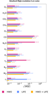 |
Fig. B.4 Square root of the mean squared error (see Equation 3) for relevant parameters in the “idealized high-resolution low-noise” retrieval set (photon noise only at S/N = 50, R = 1000). |
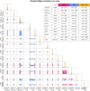 |
Fig. B.5 Corner plot for the posterior distributions from the “idealized high-resolution low-noise” retrieval set (photon noise only at S/N = 50, R = 1000). The black lines indicate the expected values for every parameter. The median and 1σ uncertainties for relevant retrieved and derived parameters are shown in the table in the top right corner. The scenarios are color-coded according to Table 3. |
When retrieving over the entire wavelength range, not only are all the species correctly retrieved, but there is a considerable increase in the precision of the retrieved estimate (a factor 2–10 on the 1σ uncertainty between a retrieval performed on only one portion of the spectrum, compared to the joint retrieval, see Fig. B.4).
Appendix C Comparison with previous works
While the current study is, to our knowledge, the first retrieval study that considers the joint performance of a direct imaging UV/VIS/NIR mission (HWO-like) together with a MIR mission (LIFE-like), many retrieval studies in the last few years have tackled the potential of future-generation instruments in characterizing Earth-like planets. We deem it useful to compare the single-instrument retrievals we performed against previous studies in the field.
C.1 HWO-like simulations
From the UV/VIS/NIR point of view, none of the previous studies can be directly compared with ours because of strong differences in the setup. However, we will discuss similarities between our results and the ones in Feng et al. (2018), Damiano & Hu (2022), Robinson & Salvador (2023), and Young et al. (2023).
The work performed in Feng et al. (2018) concerned a study on the preferred resolution and S/N to allow the characterization of an Earth twin. The authors considered an albedo model coupled with a direct-imaging noise simulator to provide the observed planet-to-star flux ratio. Their retrieval framework included cloud parameters, at the expense of a simplified atmosphere parameterization (isothermal P-T profile with only H2O, O2, O3 considered in the retrieval). The parameter estimation module used Markov Chain Monte Carlo instead of Nested Sampling. Furthermore, in Feng et al. (2018) only a wavelength range between 0.4–1.0μm was considered, at resolutions 70 and 140. Like in our “PSG and LIFESIM noise” set of retrievals, the S/N was wavelength-dependent and set to a reference value of 5, 10, 15, 20 at 0.55μm. To compare with our results, we will focus on the S/N = 10 and R = 140 results, which match the quality of the VIS band in this work.
In Feng et al. (2018) the correlation between gravity, pressure, and atmospheric abundances is also present. However, the authors notice a strong radius-albedo degeneracy, which is not noticeable in our case given the absence of clouds. Gravity and mass remain unconstrained compared to the priors in Feng et al. (2018), which is consistent with our results. In both studies H2O, O3, and O2 are detected successfully at this resolution and S/N, though wider uncertainties are present in Feng et al. (2018) compared to our study. This can be explained by the larger information content that we exploit in our retrieval, since we consider both UV and NIR wavelengths, while Feng et al. (2018) is focused on the VIS range.
Damiano & Hu (2022) performed retrievals using a reflected light forward model and considering H2O, CO2, O2, O3, and CH4 as free parameters, assuming N2 as a filler gas. In their work, the atmosphere was assumed to be isothermal and clouds were also taken into account. The authors considered a variety of scenarios: an Earth-like atmosphere, an early Earth, a CO2-dominated atmosphere with O2 and clouds, and a dry CO2-dominated atmosphere. For every scenario, they focused their attention on the information content of the NIR band to correctly characterize the atmosphere. They explored various resolutions and S/N values. The authors retrieved their error bars by fixing the S/N at the reference wavelength bin corresponding to the maximum value of the spectrum, which may vary depending on the scenarios. To compare our results with this work, we focus on the modern Earth scenario with R = 140/40 for VIS and NIR and S/N = 10, which is the closest setup to the one we simulate. These retrievals correctly identify the main components of the atmosphere (N2, O2, H2O, O3) and do not constrain CO2 and CH4, which is consistent with our results. According to the authors, to have an upper limit on the methane abundance, it would be necessary to increase the S/N to 20. Despite the differences in the parameterization of the P-T profile, also in Damiano & Hu (2022) the ground pressure is found to be overestimated.
A more recent study by Robinson & Salvador (2023) explored the detectability of an Earth twin through HabEx and LUVOIR varying the wavelength range and S/N in each band (considering three cases: optical only at S/N = 35, UV/VIS/NIR at S/N = 20, and VIS/NIR at S/N = 10/45). The authors used a single-scene albedo model for the reflected light spectrum and a constant error bar S/N whose reference points were at 0.4μm for the UV, 0.55μm for the VIS, and 1μm in the NIR. Their results on the VIS retrieval at S/N = 35 were consistent with higher S/N cases in Feng et al. (2018). As for our comparison, we discuss our results (specifically, the HWO retrieval in the simplified noise scenario) with the Robinson & Salvador (2023) retrieval on the whole UV/VIS/NIR range, which is the most similar setup despite a factor 2 difference in the S/N. The authors successfully retrieve O2, H2O, O3, and only retrieve upper limits for CO2 and CH4, in line with our results. By comparing our results with Fig. 10 in Robinson & Salvador (2023) we can observe similar variances in the posteriors of the constrained species, except for the O3 posterior. In our model, we cannot rule out abundances lower than 10−7, while the species is constrained in the earlier study. This is probably a result to be expected when increasing the S/N to 20, though such retrieval was not performed in this work.
Finally, we compare our results with a recent publication by Young et al. (2023). Here, the authors used atmospheric retrievals to identify the best observing strategy for the HWO coronagraph. They performed retrievals on various combinations of wavelength bandpass regions, defining a decision tree that would allow us to differentiate between a modern Earthlike planet and an Archean Earth-like planet. They used the same retrieval framework as Robinson & Salvador (2023) with a nominal S/N = 10 and the current baseline resolutions for the UV/VIS/NIR range (R = 7/140/70). When performing retrievals for all the considered bandpasses (three in total, centered at 0.75μm, 0.85μm, and 1.65μm with a 20% bandpass width each), Young et al. (2023) retrieve H2O, O2, and get upper limits on CO2 and CH4. This is consistent with what we find in the HWO retrievals. On the other hand, we find better constraints on the albedo and radius of the planet compared to Young et al. (2023). This is to be expected considering that our retrievals can leverage the full UV/VIS/NIR spectrum and neglect clouds, which have been known to impact these parameters. Young et al. (2023) also considered different priors on these parameters compared to our studies, which can explain the differences in the results. The mass is unconstrained (compared to the chosen prior) in both studies, and the ground temperature and pressure show similar uncertainties.
C.2 LIFE-like simulations
Regarding the MIR portion of the spectrum, we compare our results with Konrad et al. (2022); that is, LIFE Paper III. The forward model and the retrieval routine used in LIFE Paper III is overall consistent with the one used in this study, apart from the updates mentioned in Alei et al. (2022a) (LIFE Paper V) and Sec. 2.3 of this manuscript. In Konrad et al. (2022), a grid of spectral resolutions, S/N values, and wavelength ranges were explored. The S/N was calculated through LIFESIM, in a very similar way to that described in Sec. 2.1. To compare with the present work, we focus on the retrieval performed in LIFE Paper III considering R = 50, S/N = 10, and 4–18.5μm. We find very similar results between this model and the LIFE retrieval in the “PSG and LIFESIM noise” set. N2, O2, CO, N2O are unconstrained in both models. On the other hand, CO2, O3 and H2O are constrained though the mean of the posterior in our set of models is slightly shifted toward higher pressures by about 0.5 dex, a result of the slightly underestimated ground pressure that we observe in our run. In both cases, an upper limit on methane can be retrieved, though it is impossible to rule out abundances below 10−6. This happens because the methane abundance is right at the sensitivity limit of the instrument at this resolution and S/N (see Konrad et al. 2022, for more details).
The setup of the framework validation is also consistent with the “high-resolution low-noise” set of results shown in this manuscript (i.e., R = 1000, S/N = 50 only considering photon noise). The precise and accurate P-T profile retrieval in our model is consistent with the previous work, as are the estimates of the major components of the atmosphere. As was expected in the MIR, the validation run in Konrad et al. (2022) also does not detect O2 nor significantly reduces the estimate of the mass of the planet.
Appendix D Ancillary plots and tables
In this section, we collect some ancillary plots and tables. In Table D.1 we list all the parameters, the priors, and the true values assumed in the retrievals. In Tables D.2, D.3, D.4, and D.5 we show details concerning the molecular opacities, the CIA and the Rayleigh opacities used in the forward model, and the simulation settings used in LIFESIM and the PSG simulators. We report in Tables D.7 and D.8 the Bayes factor for the two baseline sets of retrievals. In Figs. D.1, and D.2 we show the corner plots and the retrieved estimates of relevant parameters for the two baseline retrieval runs.
Summary of the parameters used in the retrievals, their expected values, and their prior distributions.
References for the molecular opacities used in the retrievals.
References for the CIA and Rayleigh opacities used in the retrievals.
Simulation settings used in LIFESIM.
Simulation settings used in the PSG “6-m LUVOIR-B” simulator for each wavelength bandpass.
Physical parameters used in the noise simulation.
Bayes factor for each retrieved spectrally active species in the “simplified noise” retrieval set.
Bayes factor for each retrieved spectrally active species in the “PSG and LIFESIM noise” retrieval set.
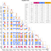 |
Fig. D.1 Corner plot for the posterior distributions from the “simplified noise” retrieval set. The black lines indicate the expected values for every parameter. The median and 1σ uncertainties for relevant retrieved and derived parameters are shown in the table in the top right corner. The scenarios are color-coded according to Table 3. |
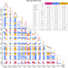 |
Fig. D.2 Corner plot for the posterior distributions from the “PSG and LIFESIM noise” retrieval set. The black lines indicate the expected values for every parameter. The median and 1σ uncertainties for relevant retrieved and derived parameters are shown in the table in the top right corner. The scenarios are color-coded according to Table 3. |
References
- Alei, E., Konrad, B. S., Angerhausen, D., et al. 2022a, A&A, 665, A106 [NASA ADS] [CrossRef] [EDP Sciences] [Google Scholar]
- Alei, E., Konrad, B. S., Mollière, P., et al. 2022b, SPIE, 12180, 121803L [Google Scholar]
- Angerhausen, D., Ottiger, M., Dannert, F., et al. 2023, Astrobiology, 23, 183 [NASA ADS] [CrossRef] [Google Scholar]
- Angerhausen, D., Pidhorodetska, D., Leung, M., et al. 2024, AJ, 167, 128 [NASA ADS] [CrossRef] [Google Scholar]
- Astropy Collaboration (Robitaille, T. P., et al.) 2013, A&A, 558, A33 [NASA ADS] [CrossRef] [EDP Sciences] [Google Scholar]
- Astropy Collaboration (Price-Whelan, A. M., et al.) 2018, AJ, 156, 123 [Google Scholar]
- Benneke, B., & Seager, S. 2013, ApJ, 778, 153 [Google Scholar]
- Bowens, R., Meyer, M. R., Delacroix, C., et al. 2021, A&A, 653, A8 [NASA ADS] [CrossRef] [EDP Sciences] [Google Scholar]
- Buchner, J., Georgakakis, A., Nandra, K., et al. 2014, A&A, 564, A125 [NASA ADS] [CrossRef] [EDP Sciences] [Google Scholar]
- Carnall, A. C. 2017, arXiv e-prints [arXiv:1705.05165] [Google Scholar]
- Carrión-González, Ó., Kammerer, J., Angerhausen, D., et al. 2023, A&A, 678, A96 [NASA ADS] [CrossRef] [EDP Sciences] [Google Scholar]
- Damiano, M., & Hu, R. 2022, AJ, 163, 299 [NASA ADS] [CrossRef] [Google Scholar]
- Dannert, F. A., Ottiger, M., Quanz, S. P., et al. 2022, A&A, 664, A22 [NASA ADS] [CrossRef] [EDP Sciences] [Google Scholar]
- Domagal-Goldman, S. D., Segura, A., Claire, M. W., Robinson, T. D., & Meadows, V. S. 2014, ApJ, 792, 90 [CrossRef] [Google Scholar]
- Dyrek, A., Ducrot, E., Lagage, P. O., et al. 2024, A&A, 683, A212 [NASA ADS] [CrossRef] [EDP Sciences] [Google Scholar]
- Feautrier, P. 1964, Comptes Rendus Academie des Sciences, 258, 3189 [NASA ADS] [Google Scholar]
- Feng, Y. K., Robinson, T. D., Fortney, J. J., et al. 2018, AJ, 155, 200 [NASA ADS] [CrossRef] [Google Scholar]
- Gaudi, B. S., Seager, S., Mennesson, B., et al. 2020, arXiv e-prints [arXiv:2001.06683] [Google Scholar]
- Gordon, I., Rothman, L., Hargreaves, R., et al. 2022, J. Quant. Spectrosc. Radiat. Transf., 277, 107949 [NASA ADS] [CrossRef] [Google Scholar]
- Greene, T. P., Line, M. R., Montero, C., et al. 2016, ApJ, 817, 17 [NASA ADS] [CrossRef] [Google Scholar]
- Hall, S., Krissansen-Totton, J., Robinson, T., Salvador, A., & Fortney, J. J. 2023, AJ, 166, 254 [NASA ADS] [CrossRef] [Google Scholar]
- Harvey, A. H., Gallagher, J. S., & Levelt Sengers, J. M. H. 1998, J. Phys. Chem. Ref. Data, 27, 761 [NASA ADS] [CrossRef] [Google Scholar]
- Hayoz, J., Cugno, G., Quanz, S. P., et al. 2023, A&A, 678, A178 [NASA ADS] [CrossRef] [EDP Sciences] [Google Scholar]
- Himes, M. D. 2022, PhD thesis, University of Central Florida, USA [Google Scholar]
- Hunter, J. D. 2007, Comput. Sci. Eng., 9, 90 [NASA ADS] [CrossRef] [Google Scholar]
- Jeffreys, H. 1998, The Theory of Probability, Oxford Classic Texts in the Physical Sciences (Oxford: Oxford University Press), 432 [Google Scholar]
- Karman, T., Gordon, I. E., van der Avoird, A., et al. 2019, Icarus, 328, 160 [Google Scholar]
- Keller-Rudek, H., Moortgat, G. K., Sander, R., & Sörensen, R. 2013, Earth Syst. Sci. Data, 5, 365 [NASA ADS] [CrossRef] [Google Scholar]
- Kofman, V., & Villanueva, G. L. 2021, J. Quant. Spectrosc. Radiat. Transf., 270, 107708 [NASA ADS] [CrossRef] [Google Scholar]
- Kokaly, R. F., Clark, R. N., Swayze, G. A., et al. 2017, USGS Spectral Library Version 7 [Google Scholar]
- Konrad, B. S., Alei, E., Quanz, S. P., et al. 2022, A&A, 664, A23 [NASA ADS] [CrossRef] [EDP Sciences] [Google Scholar]
- Konrad, B. S., Alei, E., Quanz, S. P., et al. 2023, A&A, 673, A94 [NASA ADS] [CrossRef] [EDP Sciences] [Google Scholar]
- Kozakis, T., Mendonça, J. M., & Buchhave, L. A. 2022, A&A, 665, A156 [NASA ADS] [CrossRef] [EDP Sciences] [Google Scholar]
- Krissansen-Totton, J., Olson, S., & Catling, D. C. 2018, Sci. Adv., 4 [Google Scholar]
- Latouf, N., Mandell, A., Villanueva, G., et al. 2023a, arXiv e-prints [arXiv:2311.16015] [Google Scholar]
- Latouf, N., Mandell, A. M., Villanueva, G. L., et al. 2023b, AJ, 166, 129 [NASA ADS] [CrossRef] [Google Scholar]
- Madhusudhan, N. 2018, in Handbook of Exoplanets, eds. H. J. Deeg, & J. A. Belmonte (Berlin: Springer), 104 [Google Scholar]
- Meadows, V. S., Reinhard, C. T., Arney, G. N., et al. 2018, Astrobiology, 18, 630 [Google Scholar]
- Mettler, J.-N., Konrad, B. S., Quanz, S. P., & Helled, R. 2024, ApJ, 963, 24 [NASA ADS] [CrossRef] [Google Scholar]
- Mollière, P. 2017, PhD thesis, Heidelberg University, Germany [Google Scholar]
- Mollière, P., Wardenier, J. P., van Boekel, R., et al. 2019, A&A, 627, A67 [Google Scholar]
- National Academies of Sciences, Engineering, and Medicine, 2021 (Washington, DC: The National Academies Press) [Google Scholar]
- Pandas development team, T. 2020, https://doi.org/10.5281/zenodo.3509134 [Google Scholar]
- Parviainen, H. 2018, Bayesian Methods for ExoplanetScience, ed. H. J. Deeg, & J. A. Belmonte (Cham: Springer International Publishing), 1567 [Google Scholar]
- Peterson, B. M., Fischer, D., & LUVOIR Science and Technology Definition Team. 2017, in American Astronomical Society Meeting Abstracts, 229, 405.04 [NASA ADS] [Google Scholar]
- Quanz, S. P., Crossfield, I., Meyer, M. R., Schmalzl, E., & Held, J. 2015, Int. J. Astrobiol., 14, 279 [Google Scholar]
- Quanz, S. P., Absil, O., Benz, W., et al. 2022a, Exp. Astron., 54, 1197 [NASA ADS] [CrossRef] [Google Scholar]
- Quanz, S. P., Ottiger, M., Fontanet, E., et al. 2022b, A&A, 664, A21 [NASA ADS] [CrossRef] [EDP Sciences] [Google Scholar]
- Robinson, T. D., & Salvador, A. 2023, Planet. Sci. J., 4, 10 [NASA ADS] [CrossRef] [Google Scholar]
- Sagan, C., Thompson, W. R., Carlson, R., Gurnett, D., & Hord, C. 1993, Nature, 365, 715 [NASA ADS] [CrossRef] [Google Scholar]
- Schwieterman, E. W., Kiang, N. Y., Parenteau, M. N., et al. 2018, Astrobiology, 18, 663 [CrossRef] [Google Scholar]
- Segura, A., Krelove, K., Kasting, J. F., et al. 2003, Astrobiology, 3, 689 [NASA ADS] [CrossRef] [Google Scholar]
- Sneep, M., & Ubachs, W. 2005, J. Quant. Spectrosc. Radiat. Transf., 92, 293 [NASA ADS] [CrossRef] [Google Scholar]
- Thalman, R., Zarzana, K. J., Tolbert, M. A., & Volkamer, R. 2014, J. Quant. Spectrosc. Radiat. Transf., 147, 171 [NASA ADS] [CrossRef] [Google Scholar]
- Thalman, R., Zarzana, K. J., Tolbert, M. A., & Volkamer, R. 2017, J. Quant. Spectrosc. Radiat. Transf., 189, 281 [NASA ADS] [CrossRef] [Google Scholar]
- The LUVOIR Team 2019, arXiv e-prints [arXiv:1912.06219] [Google Scholar]
- Trotta, R. 2017, arXiv e-prints [arXiv:1701.01467] [Google Scholar]
- United States committee on Extension to the Standard Atmosphere 1976, U.S. Standard Atmosphere, 1976, NOAA - SIT 76 (National Oceanic and Amospheric [sic] Administration) [Google Scholar]
- Villanueva, G. L., Liuzzi, G., Faggi, S., et al. 2022, Fundamentals of the Planetary Spectrum Generator (USA: Geronimo Villanueva) [Google Scholar]
- Voyage 2050 Senior Committee. 2021, https://www.cosmos.esa.int/documents/1866264/1866292/Voyage2050-Senior-Committee-report-public.pdf/e2b2631e-5348-5d2d-60c1-437225981b6b?t=1623427287109 [Google Scholar]
- Williams, D. M., & Gaidos, E. 2008, Icarus, 195, 927 [NASA ADS] [CrossRef] [Google Scholar]
- Young, A. V., Crouse, J., Arney, G., et al. 2023, arXiv e-prints [arXiv:2311.07530] [Google Scholar]
- Young, A. V., Crouse, J., Arney, G., et al. 2024a, Planet. Sci. J., 5, 7 [NASA ADS] [CrossRef] [Google Scholar]
- Young, A. V., Robinson, T. D., Krissansen-Totton, J., et al. 2024b, Nat. Astron., 8, 101 [Google Scholar]
All Tables
Translation table between some relevant frequentist significance values and their Bayesian interpretation, adapted from Benneke & Seager (2013) and Jeffreys (1998).
Summary of the parameters used in the retrievals, their expected values, and their prior distributions.
Simulation settings used in the PSG “6-m LUVOIR-B” simulator for each wavelength bandpass.
Bayes factor for each retrieved spectrally active species in the “simplified noise” retrieval set.
Bayes factor for each retrieved spectrally active species in the “PSG and LIFESIM noise” retrieval set.
All Figures
|
Fig. 1 Simulated observation of an Earth twin by the HWO concept assuming a simplified noise and a higher-fidelity noise instances. Top panel: the simulated observed flux at a distance of 10 pc between 0.2 and 2 μm for the two noise scenarios: simplified noise at constant error bars (shaded dark gray area with solid edges) and higher-fidelity simulated noise obtained with PSG (shaded light gray area with dotted edges). Bottom panel: signal-to-noise ratio (S/N) as a function of wavelength for the two noise instances: simplified noise (solid line) and PSG-simulated noise (dotted line). |
| In the text | |
|
Fig. 2 Simulated observation of an Earth twin by the LIFE concept assuming a simplified noise and a higher-fidelity noise instances. Top panel: simulated observed flux at a distance of 10 pc between 4 and 18.5 μm for the two noise scenarios: simplified noise at constant error bars (shaded dark gray area with solid edges) and higher-fidelity simulated noise obtained with LIFESIM (shaded light gray area with dotted edges). Bottom panel: signal-to-noise ratio (S/N) as a function of wavelength for the two noise instances: simplified noise (solid line) and LIFESIM-simulated noise (dotted line). |
| In the text | |
|
Fig. 3 Retrieved spectra for the “simplified noise” retrieval set. Left panel: pure HWO retrieval (magenta). Central panel: pure LIFE retrieval (blue). Right panel: HWO+LIFE retrieval (yellow). In all panels, the 2σ and the 1σ intervals are shown in increasingly darker hues, as well as the input spectra (black lines) with error bars (gray-shaded areas) for comparison. |
| In the text | |
|
Fig. 4 Retrieved pressure-temperature profiles for the “simplified noise” retrieval set. Left panel: pure HWO retrieval (magenta). Central panel: pure LIFE retrieval (blue). Right panel: HWO+LIFE retrieval (yellow). In all panels, the 2σ and the 1σ intervals are shown in increasingly darker hues, as well as the input profiles (black lines) for comparison. Inside each panel, the inset plot shows the 2D posterior space of the ground pressure and temperature. In all panels and the inset plots, the surface pressure and temperature point in the P-T space is shown as a red square marker. |
| In the text | |
|
Fig. 5 Posterior density distributions from the “simplified noise” retrieval set. The black lines indicate the expected values for every parameter. HWO posteriors are shown in magenta with diagonal hatching. LIFE posteriors are shown in cyan with crossed hatching. HWO+LIFE posteriors are shown as fully colored yellow histograms. |
| In the text | |
|
Fig. 6 Bayes factor and confidence levels values for each retrieved spectroscopically active species in the “simplified noise” retrieval set. The heatmap is color-coded according to the Bayes factor values log10(𝒦) and the confidence levels (in “sigma” values) are labeled within each cell whenever log10(𝒦) is positive. The Bayes factor values were obtained by performing a retrieval including and excluding the molecule of interest and then using Eq. (1). These were then converted into σ through Table 2. The Bayes factor values can be found in Table D.7. |
| In the text | |
|
Fig. 7 Square root of the mean squared error (see Eq. (3)) for relevant parameters in the “simplified noise” retrieval set. |
| In the text | |
|
Fig. 8 Retrieved spectra for the “PSG and LIFESIM noise” retrieval set. Left panel: pure HWO retrieval (magenta). Central panel: pure LIFE retrieval (blue). Right panel: HWO+LIFE retrieval (yellow). In all panels, the 2σ and the 1σ intervals are shown in increasingly darker hues, as well as the input spectra (black lines) with error bars (gray-shaded areas) for comparison. |
| In the text | |
|
Fig. 9 Retrieved pressure-temperature profiles for the “PSG and LIFESIM noise” retrieval set. Left panel: pure HWO retrieval (magenta). Central panel: pure LIFE retrieval (blue). Right panel: HWO+LIFE retrieval (yellow). In all panels, the 2σ and the 1σ intervals are shown in increasingly darker hues, as well as the input profiles (black lines) for comparison. Inside each panel, the inset plot shows the 2D posterior space of the ground pressure and temperature. In all panels and the inset plots, the surface pressure and temperature point in the P-T space is shown as a red square marker. |
| In the text | |
|
Fig. 10 Posterior density distributions from the “PSG and LIFESIM noise” retrieval set. The black lines indicate the expected values for every parameter. HWO posteriors are shown in magenta with diagonal hatching. LIFE posteriors are shown in cyan with crossed hatching. HWO+LIFE posteriors are shown as fully colored yellow histograms. |
| In the text | |
|
Fig. 11 Bayes factor and confidence levels values for each retrieved spectroscopically active species in the “PSG and LIFESIM noise” retrieval set. The heatmap is color-coded according to the Bayes factor values, log10(𝒦), and the confidence levels (in “sigma” values) are labeled within each cell whenever log10(𝒦) is positive. The Bayes factor values were obtained by performing a retrieval including and excluding the molecule of interest and then using Eq. (1). These were then converted into σ through Table 2. The Bayes factor values can be found in Table D.8. |
| In the text | |
|
Fig. 12 Square root of the mean squared error (see Eq. (3)) for relevant parameters in the “PSG and LIFESIM noise” retrieval set. |
| In the text | |
|
Fig. B.1 Best-fit spectra retrieved in the “idealized high-resolution low-noise” retrieval set (photon noise only at S/N = 50, R = 1000) for the three scenarios. Left panel: Pure HWO retrieval (magenta). Central panel: Pure LIFE retrieval (blue). Right panel: HWO+LIFE retrieval (yellow). In all panels, the best-fit spectra are compared with the input spectra (black lines) with error bars (gray-shaded areas). |
| In the text | |
|
Fig. B.2 Retrieved pressure-temperature profiles for the “idealized high-resolution low-noise” retrieval set (photon noise only at S/N = 50, R = 1000). Left panel: Pure HWO retrieval (magenta). Central panel: Pure LIFE retrieval (blue). Right panel: HWO+LIFE retrieval (yellow). In all panels, the 2σ and the 1σ intervals are shown in increasingly darker hues, as well as the input profiles (black lines) for comparison. Inside each panel, the inset plot shows the 2D posterior space of the ground pressure and temperature. In all panels and the inset plots, the surface pressure and temperature point in the P-T space is shown as a red square marker. |
| In the text | |
|
Fig. B.3 Posterior density distributions from the “idealized highresolution low-noise” retrieval set (photon noise only at S/N = 50, R = 1000). The black lines indicate the expected values for every parameter. HWO posteriors are shown in magenta with diagonal hatching. LIFE posteriors are shown in cyan with crossed hatching. HWO+LIFE posteriors are shown as fully colored yellow histograms. |
| In the text | |
|
Fig. B.4 Square root of the mean squared error (see Equation 3) for relevant parameters in the “idealized high-resolution low-noise” retrieval set (photon noise only at S/N = 50, R = 1000). |
| In the text | |
|
Fig. B.5 Corner plot for the posterior distributions from the “idealized high-resolution low-noise” retrieval set (photon noise only at S/N = 50, R = 1000). The black lines indicate the expected values for every parameter. The median and 1σ uncertainties for relevant retrieved and derived parameters are shown in the table in the top right corner. The scenarios are color-coded according to Table 3. |
| In the text | |
|
Fig. D.1 Corner plot for the posterior distributions from the “simplified noise” retrieval set. The black lines indicate the expected values for every parameter. The median and 1σ uncertainties for relevant retrieved and derived parameters are shown in the table in the top right corner. The scenarios are color-coded according to Table 3. |
| In the text | |
|
Fig. D.2 Corner plot for the posterior distributions from the “PSG and LIFESIM noise” retrieval set. The black lines indicate the expected values for every parameter. The median and 1σ uncertainties for relevant retrieved and derived parameters are shown in the table in the top right corner. The scenarios are color-coded according to Table 3. |
| In the text | |
Current usage metrics show cumulative count of Article Views (full-text article views including HTML views, PDF and ePub downloads, according to the available data) and Abstracts Views on Vision4Press platform.
Data correspond to usage on the plateform after 2015. The current usage metrics is available 48-96 hours after online publication and is updated daily on week days.
Initial download of the metrics may take a while.