| Issue |
A&A
Volume 664, August 2022
|
|
|---|---|---|
| Article Number | A23 | |
| Number of page(s) | 32 | |
| Section | Astronomical instrumentation | |
| DOI | https://doi.org/10.1051/0004-6361/202141964 | |
| Published online | 09 August 2022 | |
Large Interferometer For Exoplanets (LIFE)
III. Spectral resolution, wavelength range, and sensitivity requirements based on atmospheric retrieval analyses of an exo-Earth
1
ETH Zurich, Institute for Particle Physics & Astrophysics,
Wolfgang-Pauli-Str. 27,
8093
Zurich, Switzerland
e-mail: This email address is being protected from spambots. You need JavaScript enabled to view it.
; This email address is being protected from spambots. You need JavaScript enabled to view it.
2
National Center of Competence in Research PlanetS,
Gesellschaftsstrasse 6,
3012
Bern, Switzerland
3
Blue Marble Space Institute of Science,
Seattle,
WA, USA
4
Zentrum für Astronomie und Astrophysik, Technische Universität Berlin,
Hardenbergstrasse 36,
10623
Berlin, Germany
5
Department of Astronomy and Astrophysics, University of California,
Santa Cruz,
CA 95064
USA
6
Department of Extrasolar Planets and Atmospheres (EPA), Institute of Planetary Research (PF), German Aerospace Center (DLR),
Rutherfordstr. 2,
12489
Berlin, Germany
7
University of Bern, Center for Space and Habitability,
Gesellschaftsstrasse 6,
3012
Bern, Switzerland
8
Max-Planck-Institut für Astronomie,
Königstuhl 17,
69117
Heidelberg, Germany
9
Dept of Physics, University of Oxford,
Oxford OX1 3PU,
UK
Received:
5
August
2021
Accepted:
1
March
2022
Abstract
Context. Temperate terrestrial exoplanets are likely to be common objects, but their discovery and characterization is very challenging because of the small intrinsic signal compared to that of their host star. Various concepts for optimized space missions to overcome these challenges are currently being studied. The Large Interferometer For Exoplanets (LIFE) initiative focuses on the development of a spacebased mid-infrared (MIR) nulling interferometer probing the thermal emission of a large sample of exoplanets.
Aims. This study derives the minimum requirements for the signal-to-noise ratio (S/N), the spectral resolution (R), and the wavelength coverage for the LIFE mission concept. Using an Earth-twin exoplanet as a reference case, we quantify how well planetary and atmospheric properties can be derived from its MIR thermal emission spectrum as a function of the wavelength range, S/N, and R.
Methods. We combined a cloud-free 1D atmospheric radiative transfer model, a noise model for observations with the LIFE interferometer, and the nested sampling algorithm for Bayesian parameter inference to retrieve planetary and atmospheric properties. We simulated observations of an Earth-twin exoplanet orbiting a G2V star at 10 pc from the Sun with different levels of exozodiacal dust emissions. We investigated a grid of wavelength ranges (3–20 μm, 4–18.5 μm, and 6–17 μm), S/Ns (5, 10, 15, and 20 determined at a wavelength of 11.2 μm), and Rs (20, 35, 50, and 100).
Results. We find that H2O, CO2, and O3 are detectable if S/N ≥ 10 (uncertainty ≤ ± 1.0 dex). We find upper limits for N2O (abundance ≲10−3). In conrtrast, CO, N2, and O2 are unconstrained. The lower limits for a CH4 detection are R = 50 and S/N = 10. Our retrieval framework correctly determines the exoplanet’s radius (uncertainty ≤ ± 10%), surface temperature (uncertainty ≤ ± 20 K), and surface pressure (uncertainty ≤ ± 0.5 dex) in all cloud-free retrieval analyses. Based on our current assumptions, the observation time required to reach the specified S/N for an Earth-twin at 10 pc when conservatively assuming a total instrument throughput of 5% amounts to ≈6−7 weeks with four 2m apertures.
Conclusions. We provide first order estimates for the minimum technical requirements for LIFE via the retrieval study of an Earth-twin exoplanet. We conclude that a minimum wavelength coverage of 4–18.5 μm, an R of 50, and an S/N of at least 10 is required. With the current assumptions, the atmospheric characterization of several Earth-like exoplanets at a distance of 10 pc and within a reasonable amount of observing time will require apertures ≥ 2m.
Key words: methods: statistical / planets and satellites: terrestrial planets / planets and satellites: atmospheres
⋆ Webpage: www.life-space-mission.com
© B. S. Konrad et al. 2022
 Open Access article, published by EDP Sciences, under the terms of the Creative Commons Attribution License (https://creativecommons.org/licenses/by/4.0), which permits unrestricted use, distribution, and reproduction in any medium, provided the original work is properly cited.
1 Introduction
Since the detection of 51 Peg b, the first planetary companion to a solar-type star (Mayor & Queloz 1995), exoplanet research has become one of the pillars of modern astrophysics. With more than 4000 exoplanets currently known1, scientists have begun to uncover the vast diversity among exoplanet objects and extrasolar systems. A long-term goal is the discovery and the atmospheric characterization of a large sample of terrestrial exoplanets, with a specific focus on temperate objects.
In this context, a direct detection approach is essential in order to investigate the diversity of planetary atmospheres, assess the potential habitability of some objects, and look for biosignatures in their atmospheres. Different concepts for large exoplanet imaging space missions are currently being assessed, with LUVOIR (Peterson et al. 2017) and HabEx (Gaudi et al. 2020), which aim to directly measure the reflected spectrum of exoplanets in the visible (VIS) and near-infrared (NIR) range, being prominent examples. The Large Interferometer For Exoplanets (LIFE) initiative2 follows a complementary approach by focusing on the prospects of a large, space-based mid-infrared (MIR) nulling interferometer, which will observe the thermal emission spectrum and subsequently characterize the atmospheres of a large sample of (terrestrial) exoplanets (Quanz et al. 2018, 2021, 2022). The LIFE initiative aims to combine various efforts to push toward an eventual launch of such a large, space-based MIR nulling interferometer. The work we present here aims to constrain some of the instrument requirements for LIFE and it is the third paper in a series. The first paper of the series (Quanz et al. 2022) quantifies the exoplanet detection performance of LIFE and compares it with large single-aperture mission concepts for reflected light. The second paper (Dannert et al. 2022) introduces the LIFEsim instrument simulator and the necessary signal extraction algorithms.
The choice of the MIR wavelength range for LIFE pays dividends. More molecules have strong absorption bands in the MIR spectra of Earth-like planets, which allows us to better assess the atmospheric structure and composition (e.g., Des Marais et al. 2002; Line et al. 2019). Further, the infrared is less affected by the presence of hazes and clouds (see, e.g., Kitzmann et al. 2011; Rugheimer et al. 2013; Arney et al. 2018; Lavvas et al. 2019; Fauchez et al. 2019; Komacek et al. 2020; Wunderlich et al. 2021), which is a major challenge at visible wavelengths (see, e.g., Sing et al. 2016, for Jovian planets)3. Importantly, emission spectra allow us to constrain the planetary radius (e.g., Line et al. 2019), which is degenerate with the planetary albedo in reflected light measurements (Carrión-González et al. 2020).
Finally, the MIR range includes a rich portfolio of biosignatures (e.g., Catling et al. 2018). Biosignatures in an exoplanet context are gases or features that can be detected at interplanetary distances and that are produced by life. Among the main biosignature gases there are oxygen (O2) and its photochemical product ozone (O3), methane (CH4), nitrous oxide (N2O), chloromethane (CH3Cl), phosphine (PH3), and dimethyl sulfide (C2H6S, commonly known as DMS). Many of these gases can also be generated by abiotic processes and can therefore be false positives in the search for biosignatures (Schwieterman et al. 2018; Harman & Domagal-Goldman 2018). However, the presence of multiple biosignature gases in the atmosphere, along with a planetary context that points toward habitability, would increase the robustness of the detection of life on an exoplanet. The most widely known set of multiple biosignatures is the so-called triple fingerprint of carbon dioxide (CO2), water vapor (H2O), and O3, which are well detectable in Earth’s thermal emission spectrum and potentially detectable in terrestrial exoplanets (see, e.g., Selsis et al. 2002). The simultaneous presence of reducing and oxidizing species in an atmosphere, such as O2 and O3 in combination with CH4, is a strong biosignature, with no currently known false positives. These species would not be both present in large quantities in an atmosphere over long timescales without disequilibrium processes driven by the presence of life (Lederberg 1965; Lovelock 1965). An exhaustive discussion on biosignatures can be found in Schwieterman et al. (2018) and Catling et al. (2018) introduce a Bayesian framework for assessing the confidence level of a biosignature detection.
While there is ample scientific justification for choosing the MIR wavelength regime for detailed (atmospheric) investigations of terrestrial exoplanets, deriving a concept for a space-mission, as pursued by the LIFE initiative, requires the derivation of fundamental mission and instrument requirements, including instrument sensitivity, wavelength range coverage, and spectral resolution. Earlier steps in this direction were presented in von Paris et al. (2013) for the former Darwin mission concept (Léger et al. 1996). In a more recent study, Feng et al. (2018) used a Bayesian atmospheric retrieval approach to quantify the power of reflected light observations, as foreseen by HabEx or LUVOIR, as a function of instrument parameters.
Here, we aim to provide the minimum requirements for the parameters listed above for the LIFE mission concept using an atmospheric retrieval framework. Such a framework allows us to derive quantitative estimates for the main atmospheric and planetary parameters from a simulated exoplanetary spectrum (see, e.g., Madhusudhan 2018; Deming et al. 2018; Barstow & Heng 2020, for recent reviews). Using a Bayesian approach, the space of input parameters (e.g., atmospheric abundances) is explored iteratively to assess which combination of values best fits the simulated observations. Repeating this for various combinations of signal-to-noise ratio (S/N) of the emission spectrum, wavelength range, and spectral resolution (R) allows us to understand, how well the simulated planet can be characterized. In the present study, we used a cloud-free modern Earth-twin exoplanet as our reference case. As Earth is the only planet known to host life, we are particularly interested in assessing if and how well some of its main atmospheric constituents can be detected for various combinations of instrument parameters. We are aware that by ignoring clouds, we are somewhat simplifying the problem. However, we emphasize here that the main aim of our analysis is to get first estimates for wavelength range coverage, R, and S/N requirements for LIFE. In subsequent work, we will investigate other types of exoplanets and atmospheric compositions, providing additional constraints on some of the requirements.
In Sect. 2, we introduce our retrieval framework. It combines a 1D atmospheric forward model based on the petitRADTRANS radiative transfer code (Mollière et al. 2019), the LIFEsim instrument simulator (Dannert et al. 2022), that adds astrophysical noise terms to the simulated Earth spectrum, and a Nested Sampling approach (Skilling 2006) for Bayesian parameter inference. We validate the retrieval framework in Sect. 3. Then, we perform a series of retrievals of the theoretical emission spectrum of a cloud-free Earth-twin exoplanet as it would be observed by LIFE, varying the wavelength range coverage, R, and S/N. We present our results in Sect. 4. In Sect. 5, we discuss our results and compare our study with other works. Finally, we summarize our main findings and conclusions in Sect. 6.
2 Methods
Our atmospheric retrieval framework aims to infer the atmospheric pressure-temperature (P−T) structure and composition from simulated mock observations of the MIR thermal emission spectrum of an Earth-twin planet. At its heart, the framework consists of two elements. First, we need a parametric model for the atmosphere that calculates the emergent light spectrum corresponding to a set of model parameters (Sect. 2.1). Second, a parameter estimation algorithm is required to optimize the model parameters, such that the spectrum produced by the atmospheric model best fits the simulated observational data (Sect. 2.2). These two elements are then combined to form our retrieval framework (Sect. 2.3). We provide an illustrative schematic summarizing our retrieval framework in Fig. 1.
 |
Fig. 1 Schematic illustrating our atmospheric retrieval framework. |
2.1 Atmospheric Model
As our atmospheric model, we used the 1D radiative transfer code petitRADTRANS (Mollière et al. 2019). To calculate the thermal emission spectrum of terrestrial exoplanets in the MIR wavelength range, petitRADTRANS passes a featureless black-body spectrum at the surface temperature through discrete atmospheric layers that interact with the radiation field. We characterized each layer by its temperature, pressure, and the opacity sources present.
2.1.1 Atmospheric P–T Structure
Throughout this work, we parametrized the P−T structure of Earth’s atmosphere using a fourth order polynomial:
 (1)
(1)
Here, P denotes the atmospheric pressure and T the corresponding temperature. The parameters ai are the parameters describing the polynomial P−T model. We chose this polynomial P−T model over other P−T profile parametrizations (e.g., models from Madhusudhan & Seager 2009; Guillot 2010; Mollière et al. 2019), since it provided a comparable description of the atmospheric P−T structure using fewer model parameters (see Appendix A for further information).
2.1.2 Opacity Sources in PetitRADTRANS
With petitRADTRANS, we can account for several different opacity sources that are potentially present in exoplanet atmospheres. In the computationally favorable low spectral resolution mode (R = 1000), the opacities originating from different atmospheric gases are calculated via the correlated-k method (Goody et al. 1989; Lacis & Oinas 1991; Fu & Liou 1992). Absorption lines from different molecules, collision-induced absorption (CIA), and atmospheric pressure broadening effects can be taken into account. Rayleigh and cloud scattering, as well as the scattering of direct radiation from the host star, can be considered. However, the scattering solution is achieved in an iterative way and the opacity handling is different (see Mollière et al. 2020, for more information). These changes increase the spectrum calculation time by roughly an order of magnitude when scattering is included in the computation.
In Fig. 2, we compare our scattering- and cloud-free Earth-twin MIR emission spectrum, for which we assumed uniform chemical abundances throughout the atmosphere, to other cloud-free and cloudy models (Daniel Kitzmann, priv. comm.; Rugheimer et al. 2015). These models considered scattering as well as nonuniform abundances. We see that scattering contributions and nonuniform abundances only have a minor impact on Earth’s spectrum in the MIR and the differences between the cloud-free spectra are of similar magnitude as the most optimistic LIFEsim noise estimate. This justifies our approach of excluding scattering from our retrieval routine. Thus, we neglected effects linked to the incident stellar radiation, which reduces the number of retrieved parameters and thereby the computing time.
We also neglected scattering and absorption by clouds. As can be seen from Fig. 2, this is a significant simplification of the problem. The presence of (opaque) clouds in an atmosphere will partially or fully obscure the view of the exoplanet’s surface. Therefore, we expect systematic shifts in the surface temperature, pressure, and potentially also in the retrieved planetary radius if clouds are present in an atmosphere. Additionally, a partial cloud coverage combined with vertically nonconstant atmospheric abundances could lead to systematic offsets in the retrieved abundances. For example, if an atmospheric gas is only present below an optically thick cloud deck, it is likely not detectable via a MIR retrieval study. These considerations require further attention in future works. However, as we are interested in first estimates for specific instrument requirements, focusing on a cloud-free atmosphere is justifiable. Complete details on the implementation are given in Sect. 2.3.1.
 |
Fig. 2 Comparison of the Earth-twin MIR emission spectra calculated with various different models. We plot the photon flux received from an Earth-twin located 10 pc from the sun. The solid blue line is the MIR thermal emission calculated with petitRADTRANS using the settings discussed in Sect. 2.3.1. The blue-shaded region indicates the most optimistic LIFEsim uncertainty (S/N = 20) used in our retrievals. The red dashed line represents a cloud-free Earth model by Daniel Kitzmann (priv. comm.), which takes scattering into account. The green and black dashed-dotted lines are the cloudy (60% cloud coverage) and cloud-free modern Earth spectra from Rugheimer et al. (2015) that account for scattering. |
2.2 Parameter Estimation
Our retrieval study utilized a Bayesian parameter inference tool to sample the posterior probability distributions of the atmospheric forward model parameters. Bayesian parameter inference methods are based on Bayes’ theorem, which provides a method for estimating model parameters based on experimental data (see, e.g., Trotta 2017; van de Schoot et al. 2021). Let us consider a model ℳ described by a set of parameters Θℳ and experimental data Ɗ. Bayes’ theorem states:
 (2)
(2)
Here, P(Θℳ∣Ɗ, ℳ) is the posterior probability (or “posterior”) and represents the probability of different sets of model parameters Θℳ under the constraint of the experimental data Ɗ and model ℳ. Further, P(Ɗ∣Θℳ, ℳ) provides a probabilistic measure of how well a specific set of parameters Θℳ for the model ℳ describes the data Ɗ. We calculated this probability via a log-likelihood function ln (ℒ(Θℳ)):
 (3)
(3)
Our log-likelihood function assumed that each of the N measured data points Ɗi behaves as a normally distributed quantity. The mean μi (Θℳ) was assumed to be the value predicted by the model ℳ using parameters Θℳ. The variable σi was the measurement error on the data point Ɗi.
Next, P(Θℳ∣ℳ) is the prior probability (or “prior”) of the model parameters Θℳ and represents the knowledge on the model parameters before taking the observational data into account. Finally, P(Ɗ∣ℳ) is frequently referred to as the Bayesian evidence  and is a normalization constant, which ensures that the posterior is normalized to unity:
 (4)
(4)
Additionally, the evidence  enables us to compare the performance of different models ℳi to each other and to select the model that best describes the observed data Ɗ. One can compare two models ℳ1 and ℳ2 by considering the Bayes’ factor K:
 (5)
(5)
where the prior probabilities P(ℳi) for both models are assumed to be the same. An approach to interpreting the value of K is via the Jeffrey’s scale (Jeffreys 1998), which is given in Table 1.
Due to the model comparison capabilities of the evidence  , we chose the nested sampling algorithm (Skilling 2006) over MCMC algorithms (e.g., the Metropolis-Hastings algorithm: Hastings 1970; Metropolis et al. 1953), since it provides a direct estimate for the Bayesian evidence
  . Furthermore, nested sampling is computationally less expensive and better at handling multimodal posterior distributions (Skilling 2006).
Specifically, we utilized the open-source pyMultiNest package (Buchner et al. 2014), which makes the nested sampling implementation MultiNest (Feroz et al. 2009) accessible to the Python language. MultiNest is based on the original nested sampling algorithm (Skilling 2006) and uses the importance nested sampling algorithm (Feroz et al. 2013) to obtain more accurate estimates of the Bayesian evidence  .
.
Jeffrey’s scale (Jeffreys 1998).
 |
Fig. 3 Wavelength dependence of different opacity sources. Upper panel: the opacity of a cloudless Earth-twin atmosphere as a function of wavelength. Gray shading shows the amount of light blocked by the atmosphere. Lower panel: contribution of the different molecules to the opacity of the Earth-twin atmosphere as a function of wavelength. Dark regions indicate a high opacity, as is indicated by the colorbar. |
Line lists used throughout this study.
2.3 Retrieval Setup
2.3.1 Forward Model and Noise Terms
We generated a correlated-k petitRADTRANS spectrum (R= 1000) of an Earth-twin exoplanet using the parameter values listed in Table 3 (Input column) assuming an atmosphere consisting of 100 layers. We used the line lists from the ExoMol database (Tennyson et al. 2016) for CO2, CH4, and N2O and from the HITRAN/HITEMP database (Rothman et al. 1995, Rothman et al. 2010) for O3, CO, and H2O. We summarize the reference papers corresponding to the opacity line lists in Table 2. For N2 and O2, we considered CIA (as discussed in Schwieterman et al. 2015). All other atmospheric gases have distinct absorption features within the MIR range, even at low abundances (see Fig. 3). Furthermore, we assumed constant abundances of all molecules vertically throughout the atmosphere.
We then resampled the calculated MIR emission spectrum to the desired spectral resolution, keeping a constant resolution R = λ/∆λ across the spectrum. This resulted in wavelength bins of variable width, where the width at short wavelengths was smaller than at long wavelengths. For the spectral resampling, we used the SpectRes tool (Carnall 2017), which allows for time efficient resolution reduction of MIR spectra whilst keeping the overall flux and energy conserved. We then used the radius Rpl and the distance from Earth dEarth to scale the photon flux found with petitRADTRANS FpRT to the flux LIFE would detect (Flife):
 (6)
(6)
Throughout this work, we defined the S/N of a spectrum as the S/N calculated in the reference bin at 11.2 μm. We chose this wavelength because it lies close to the peak flux and it does not coincide with strong absorption lines. The S/N at all other wavelengths was determined by the noise model, which relates the S/N for the reference bin to the S/N in all other wavelength bins.
For the retrieval validation we perform in Sect. 3, we only considered the photon noise of the planet spectrum. For the grid retrievals performed in Sect. 4.2, we obtained noise estimates via the LIFEsim tool (see Dannert et al. 2022). LIFEsim accounts for photon noise contributions from the planet’s emission spectrum, stellar leakage, as well as local- and exozodiacal dust emission. In our simulations, we assumed that the noise did not impact the predicted flux values, but instead only added uncertainties to the simulated spectral points. As discussed in Feng et al. (2018), randomization of the individual spectral points based on the S/N allows us to simulate accurate observational instances. At the same time, retrieval studies on such instances result in biased results, since the random placement of the small number of data points will impact the retrieval’s performance. The ideal analysis would study many (at least 10) data realizations for each considered spectrum and assess instrument performance by considering the posteriors found for these different noise instances. However, the number of cases (96) we considered and the computation time per case (≈1 day on 90 CPUs) made such a study computationally unfeasible (≳30 months of cluster time). By not randomizing the individual spectral points, we eliminated the biases introduced by noise instances. However, we are aware that this approach likely leads to overly optimistic results. Namely, we expect an unrealistic centering of posteriors on the truths. Additionally, for molecules at the sensitivity limit (weak spectral features), we expect overly optimistic results (see, e.g., Feng et al. 2016). In Appendix C, we performed retrievals on randomized noise instances to study these effects in more detail.
Parameters used in the retrievals, their input values, prior distributions, and the validation results.
2.3.2 Priors
We provide the assumed prior ranges for all model parameters in Table 3. For the polynomial P−T profile and the surface pressure P0, we chose priors that cover a wide range of atmospheric structures. The prior range included Venus- or Mars-similar atmospheric structures (e.g., P0 is considered over the range from 10−4 to 1000bar, as indicated by  .
.
As demonstrated in Dannert et al. (2022), the detection of a planet during the search phase of the LIFE mission will already provide first estimates for the radius Rpl of the object. Specifically, for small, rocky planets within the habitable zone, the authors showed that a detection in the search phase would provide an estimate Rest for the true planet radius Rtrue with an accuracy of Rest/Rtrue = 0.97±0.18. For our simulations, we therefore assumed that a rough estimate of the radius is known and we chose a Gaussian prior with 20% uncertainty for this parameter. Next, we used the Rpl to derive a constraint on the planet’s mass Mpl via a statistical mass-radius relation (see, e.g., Hatzes & Rauer 2015; Wolfgang et al. 2016; Zeng et al. 2016; Chen & Kipping 2016; Otegi et al. 2020). In our retrievals, we used Forecaster4 (Chen & Kipping 2016), which allowed us to set a prior on the planetary mass Mpl based on the estimate for the radius Rpl. The tool relies on the statistical analysis of 316 objects (Solar System objects and exoplanets) for which well-constrained mass and radius estimates are available. It produces accurate predictions for a large variety of different objects, spanning from dwarf planets to late-type stars.
For the trace gases, we assumed uniform priors between −15 and 0 in log10 mass fraction. For the bulk constituents N2 and O2, we used uniform priors between −3 and 0 in log10 mass fraction. This range gave us an increased sampling density in the high abundance regime, where we expected the sensitivity limit to be located for N2 and O2. Furthermore, we used N2 as filling gas in our atmosphere, to ensure that: ∑ (gas abundances) = 1.
3 Validation
Before running our retrieval framework for simulated LIFE data, we validated its accuracy and performance. For the retrieval validation, we retrieved a full resolution (R = 1000) Earth-twin MIR thermal emission spectrum covering the wavelength range 3−20 μm. We generated the validation input spectrum using petitRADTRANS and the parameter values provided in Table 3. We only considered photon noise from the spectrum itself and chose an S/N of 50 at 11.2 μm. Furthermore, we assumed that the photon noise did not impact the simulated flux values, but instead only added uncertainties to the spectral points. In our validation retrieval, we ran the pyMultiNest package using 700 live points and a sampling efficiency of 0.3 as suggested for parameter retrieval by the documentation5.
We summarize the results in Fig. 4 and Table 3 (last column). The corner plot in Fig. 4a suggests that the exoplanet’s radius Rpl is retrieved to a very high precision with an uncertainty of roughly 0.001 R⊕, a significant improvement over the assumed prior distribution. Similarly, the retrieved posterior for the exoplanet mass Mpl is more strongly constrained than the assumed prior distribution, with the standard deviation of the posterior (0.2 · log10(M⊕)) being significantly smaller than the standard deviation of the prior (0.4 · log10(M⊕)). The centering of the Rpl and Mpl posteriors on the true values and the lack of significant correlation between the two posteriors implies that the surface gravity gp1 is estimated accurately. The surface pressure P0 and surface temperature T0 are both accurately retrieved to a very high precision, with an uncertainty of roughly 0.1 K for T0 and 0.1 bar for P0 (see Figs. 4a and 4b). Further, we observe a correlation between the planetary radius Rpl and the surface temperature T0. This indicates that a higher T0, which results in more emission per surface area, can be compensated by a smaller Rpl, which results in a smaller emitting area.
From the retrieved posterior distribution of N2, we see that our retrieval framework allows us to rule out low N2 abundances in Earth’s atmosphere via the N2−N2 CIA feature at 4 μm. However, the same N2-N2 CIA feature is too weak to rule out very high N2 abundances. In contrast, the retrieval did not manage to find evidence for O2 in Earth’s atmosphere. However, the retrieval managed to limit the O2 abundance to maximally 0.35 in mass fraction.
The retrieved posterior distributions for the remaining molecules show a strong correlation with the Mpl posterior and consequently with the surface gravity gp1. This correlation is evident in the corner plot of Fig. 4a since both Mpl and the molecular abundances of most retrieved trace gases exhibit a similarly shaped, non-Gaussian posterior distribution. This is a well known physical degeneracy and has been described in other studies (see, e.g., Mollière et al. 2015; Feng et al. 2018; Madhusudhan 2018; Quanz et al. 2021); it is not related to a numerical artifact. The degeneracy appears since the same spectral feature can be explained by different combinations of gravity and atmospheric composition. This degeneracy originates from the mass appearing in the form of the surface gravity in the hydrostatic equilibrium. Therein, the surface gravity is degenerate with the mean molecular weight of the atmospheric species. Since we derive the mean molecular weight from the abundances of the trace gases, this connects the planet’s mass to the trace gas abundances present in its atmosphere. Further evidence for this degeneracy can be found in Fig. 4c. Despite the degeneracy between the retrieved mass and molecule abundances, the relative difference between the input spectrum and the spectra corresponding to the retrieved parameters is small.
The posteriors of CO and N2O are broader, roughly Gaussian, and less correlated with Mpl. This indicates that the constraint imposed by the retrieval framework on the abundances of these species is not solely limited by the degeneracy with Mpl, but also by our retrieval’s sensitivity for CO and N2O.
A method of dealing with these strong correlations is to consider relative instead of absolute abundances. This allows us to minimize the impact of systematic uncertainties that affect all retrieved trace gas abundances in the same way at the cost of losing information on the absolute abundances. Relative abundances of trace gases are of interest to us since they provide a probe to whether an atmosphere is in chemical disequilibrium, which could potentially be upheld by life. For example, we could consider the abundance of CH4 or N2O relative to a strongly oxidizing species such as O2 (or O3, which is a photochemical product of O2) as first suggested in Lovelock (1965) and Lippincott et al. (1967). These gases react rapidly with each other and therefore the simultaneous presence of both molecules is only possible if they are continually replenished at a high rate. On Earth, O2 is constantly produced via photosynthesis and there is a continuous flux of CH4 into the atmosphere due to biological methanogenesis and anthropogenic methane production. Similarly, the N2O in Earth’s atmosphere is continually replenished by a large range of microorganisms via incomplete denitrification. On Earth, these biological processes lead to CH4 and N2O abundances that are many orders of magnitude larger than the chemical equilibrium. Another interesting ratio of atmospheric gases to consider is the ratio between CO and CH4. A large amount of CO accompanied by a lack of significant CH4 could be interpreted as an antibiosignature as suggested in Zahnle et al. (2008). A more exhaustive discussion of potential biosignatures can be found in Schwieterman et al. (2018), for example.
The retrieved P−T structure is displayed in Fig. 4b. Our retrieval framework extracts the P−T structure of Earth’s lower atmosphere accurately to very high precision. With decreasing pressure, the uncertainty on the retrieved P−T profile increases due to a lack of signatures from the low-pressure atmospheric layers (≲10−4 bar) in the exoplanet’s emission spectrum.
 |
Fig. 4 Results from the validation run outlined in Sect. 3. (a) Corner plot for the posterior distributions of the planetary surface temperature T0, surface pressure P0, radius Rpl, mass Mpl, and retrieved abundances of different molecules. The red lines indicate the values used to generate the input spectrum. Additionally, we plot the retrieved median and the 16th and 84th percentile as dashed lines in every posterior plot. (b) Retrieved P−T profile. The shaded green regions show the uncertainties on the retrieved profile. In the bottom left corner of the P−T profile plot, we display P0 and T0. The red cross marks the input values. (c) The retrieved emission spectrum Fretrieved relative to the input emission spectrum for the retrieval Finput. |
4 Results
In the following, we analyze the performance of the retrieval suite in characterizing an Earth-twin planet orbiting a Sun-like star at 10 pc from our Earth. We first estimate the fundamental detection limits of our retrieval suite for the trace gas abundances for different input spectra, as described in Sect. 4.1. We then introduce the full grid of retrievals that was run in Sect. 4.2. The results are presented in Sects. 4.3 and 4.4.
4.1 Detection Limit Analysis
We define the fundamental detection limits of our retrieval suite as the lowest possible molecular abundances that are retrievable for the atmospheric gases considered. For abundances below the detection limit, the corresponding spectral features are lost in the observational noise. Specifically, we estimate the detection limits of the trace gases considered in our retrievals at different values for R (20, 50, 1000), S/N (10, 20, 50), and for the largest and smallest assumed bandwidth (3−20 μm, 6−17 μm).
To do so, we generated spectra from the parameter values listed in Table 3, but set the abundance of one trace gas to 0 for each generated spectrum. We then used these spectra as retrieval input, assumed only photon noise of the planet to be present, and retrieved for the absent trace gas. We passed all other model parameters to the retrieval as known.
By construction, the retrieval routine should rule out any abundance of the missing gas down to the detection limit abundance, where the spectral features are no longer distinguishable from the noise. The posterior distribution should therefore be a flat distribution (all values are equally probable) for abundances smaller than the threshold value. For values greater than the detection limit, the probability should be close to null. The threshold value can therefore be interpreted as a detection limit for the gas abundance.
We approximated the retrieved posterior for the trace gas abundance as a logistic function (a soft step function):
 (7)
(7)
Here, x is the abundance of the trace gas for which the detectability is being considered. The constants a, b, and c are unique for each posterior. In Table 4, we provide the abundances corresponding to the half maximum and the 16th and 84th percentile of the fitted logistic function for all tests we ran. The half maximum together with the percentiles provides an estimate for the detection limit of our retrieval suite.
The results for the R = 1000 test case predict that all atmospheric trace gases should be detectable in such a retrieval. This is in agreement with the validation results presented in Sect. 3. For the cases where R ≤ 50, we predict H2O, CO2, and O3 to be easily detectable in an Earth-like atmosphere, since the true abundances are more than one order of magnitude larger than the retrieval’s estimated detection limit. For CH4, the true abundance is comparable to the retrieval’s detection limit. Thus, we expect the performance for CH4 to depend strongly on the R and S/N of the input spectrum. The true CO and N2O abundances lie at least one order of magnitude below the estimated detection limits and are therefore irretrievable. The upper limit of CO exhibits a strong dependence on the wavelength range considered because the only CO feature in the MIR is located at ~4.7 μm (see Fig. 3). Excluding the 3−6 μm wavelength range from the analysis makes the CO abundance impossible to constrain.
This test study has provided best case detection limits for the abundance in Earth-like atmospheres. However, retrieval of all parameters will lead to an overall increase in these detection limits. Additionally, adding additional astrophysical noise terms will also negatively impact the detection limits for the trace gases.
Retrieval sensitivity analysis results.
4.2 Retrieval Grid
We chose to consider the following grid of wavelength ranges, R values, and S/N values in our final grid of retrieval studies:
Wavelength ranges: 3–20 μm, 4–18.5 μm, and 6–17 μm.
Spectral resolutions: R = 20, 35, 50, and 100.
Signal-to-noise ratios: S/N =5, 10, 15, and 20 fixed at the wavelength bin centered at 11.2 μm.
The short end of the wavelength range tests, whether the CO band at ~4.7 μm can be retrieved and whether including the ~3.3 μm band of CH4 helps with the detection of this molecule. At the long wavelength end, the main question is how much of the extended H2O feature should be included in the analysis. The choice for the spectral resolution range was motivated by earlier studies (e.g., Des Marais et al. 2002).
For the reference planet, we again assumed the thermal emission spectrum of an Earth-twin in orbit around a G2V star located at a distance of 10 pc from Earth. We considered two observational cases with slightly different noise properties and observational setups:
Nominal case: (1) the LIFE baselines (physical distance between the four mirrors) were optimized for the detection of habitable zone planets at a wavelength of λ = 15 μm (cf. Quanz et al. 2022); (2) the level of exozodiacal dust emission corresponded to three times the level of the local zodiacal light.
Optimized case: (1) the LIFE baselines were optimized for the detection of habitable zone planets at the short wavelength end; (2) the level of exozodiacal dust emission corresponded to 0.5 times the level of the local zodiacal light6.
Figure 5 visualizes the difference between the nominal and the optimized S/N case by plotting the ratio between the two S/N instances. We computed the full noise terms (including stellar leakage, local zodi and exozodi emission, and photon noise from the planet) using LIFEsim (see Dannert et al. 2022). In total, the grid comprised 96 retrieval analyses. Figure 6 visualizes the highest (R = 100’ S/N = 20) and lowest (R = 20, S/N = 5) quality input spectra for the nominal case. For every grid point specified above, we ran one retrieval assuming the prior distributions listed in Table 3. Furthermore, we used the same pyMultiNest settings applied in the retrieval validation run (Sect. 3).
Taking the 3–20 μm nominal case input spectra as an example, we plot the posteriors of the planetary parameters (Fig. 7), as well as those for the absolute (Fig. 8) and the relative (Fig. 9) abundances. We use the retrieved posterior probability distributions to underline trends with respect to the wavelength range, R, and S/N. For the molecular abundances, we differentiate between four different classes of posterior distributions. First, a constrained (C-type) posterior signifies that the true atmospheric abundance lies above the retrieval’s detection limit. A C-type posterior is well approximated by a Gaussian. Thus, both significantly higher and lower abundances are ruled out. Second, for a sensitivity limit (SL-type) posterior, the true atmospheric abundance is comparable to the detection limit of the retrieval. We observe a distinct peak in the posterior. However, lower abundances cannot be fully ruled out. A SL-type posterior is best described by the convolution of a logistic function with a Gaussian. Third, a upper limit (UL-type) posterior indicates that the true atmospheric abundance lies below the retrieval’s detection limit and could be zero. A UL-type posterior is best described by the logistic function introduced in Sect. 4.1. Abundances above the detection limit can be excluded, while all abundances below the limit are equally likely. Fourth, an unconstrained (UC-type) posterior signifies that no information about the atmospheric abundance can be retrieved. The posterior is best described by a constant function. For more detailed information about our posterior classification, see Appendix B.
Figure 10 summarizes the type of the retrieved posterior distribution for the molecular abundances for all considered R, S/N, wavelength ranges, and the two different cases. Tables containing the median as well as the 16th and 84th percentile of the retrieved posteriors for all retrieval runs are provided in the Appendix D (Tables D.1–D.6).
 |
Fig. 5 Ratio between the wavelength-dependent S/N of the optimized case and the nominal case. This ratio is independent of the overall S/N and the R of the Spectrum. |
 |
Fig. 6 Examples of input spectra used in the grid retrievals for the nominal case (left: the lowest quality input with R = 20, S/N = 5; right: the highest quality input with R = 100, S/N = 20). In gray, we provide the full resolution petitRADTRANS Earth spectrum. The red step function represents the wavelength-binning of the input data. Further, the blue shaded region represents the uncertainty for the corresponding bin. We also mark the absorption features of the considered atmospheric gases. |
 |
Fig. 7 Retrieved exoplanet parameters for the different grid points for the wavelength range 3–20 μm in the nominal case. Here, Mpl is the mass, Rpl the radius, P0 the surface pressure, and T0 the surface temperature of the exoplanet. The error bars denote the 68% confidence intervals. For Mpl and Rpl, we also plot the assumed prior distributions. For T0 and P0, we assumed flat, broad priors. The vertical lines mark the true parameter values. |
4.3 Retrieved Planetary Parameters
In Fig. 7, we provide the retrieval results for the exoplanet parameters Mpl, Rpl, P0, and T0 (3–20 μm input spectra in the nominal case). Our retrieval framework estimates all planetary parameters correctly.
For the planetary mass Mpl, the retrieved posterior is centered on the true value and roughly corresponds to the assumed prior distribution. This result indicates that our retrieval framework cannot extract further information from the input spectrum. In contrast to Mpl, we manage to strongly constrain the exo-planet’s radius Rpl with respect to the assumed prior distribution. For all S/N ≥ 10, we retrieve an accurate estimate for Rpl (∆Rpl ≤ ± 10%).
For all S/N ≥ 10, our retrievals yield strong constraints for the surface pressure P0. The retrieved value lies within maximally ± 0.5 dex (a factor of ≈ 3) depending on the R and S/N combination. Similarly, the surface temperature T0 (calculated from the retrieved P–T profile parameters and P0) is accurately estimated by our retrieval framework for all S/N ≥ 10. The retrieved values are centered on the correct value for most cases and the 1σ uncertainties are mostly smaller than ± 20 K.
For an S/N of 5, the retrieved parameters T0 and P0 exhibit significant offsets with respect to the input value. Furthermore, we find similar offsets for Rpl. These deviations indicate that an S/N of 5 is too low for the accurate characterization of an Earth-twin exoplanet’s atmospheric structure, as we discuss further in Sect. 4.4. The same is true for all other wavelength ranges and both the nominal and the optimized cases considered in our work (see Appendix D).
4.4 Retrieved Abundances
The retrieved molecular abundances of the atmospheric trace gases are provided in Fig. 8 (3–20 μm input spectra for the nominal case). We observe that the abundances of CO2, H2O, and O3 are accurately retrieved to a precision of ≤ ± 1 dex for all cases where the S/N is ≥ 10. In contrast, the molecule CH4 only becomes retrievable for high combinations of R and S/N (for S/N = 10 at R ≥ 100, for S/N = 15 at R ≥ 50, and for S/N = 20 a R ≥ 35). For other combinations of R and S/N, we only retrieve upper limits on the CH4 abundance.
The CO abundance is not constrained by our retrievals for any S/N ≥ 10. At an S/N of 5 we retrieve an upper limit on the abundance of CO. This upper limit is a result of the poor overall retrieval performance in the S/N = 5 case as we motivate below. Similarly, we do not retrieve the N2O abundance, but find an upper limit for the maximal possible abundance. The position of this upper limit decreases significantly with increasing R and S/N of the input spectrum. Further, the input spectra do not contain sufficient information to constrain the abundances of the bulk constituents N2 and O2 for all considered R and S/N combinations (not shown). We retrieve UC-type posteriors and cannot provide any constraint for N2 and O2 in our retrievals.
Finally, by adding up the retrieved abundances, we find that there is at least one additional atmospheric gas that has no MIR signature probable by LIFE, constitutes ≈ 99% of Earth’s atmospheric mass, and has no significant absorption feature in the MIR. We can exclude H and He dominated atmospheres due to the small retrieved radius and CO2, CH4, or H2O dominated atmospheres due to our retrieval results. These findings already put strong constraints on the bulk atmospheric composition.
Overall, the findings we presented agree well with the predictions obtained in the sensitivity analysis (Sect. 4.1). This indicates that the simplified assumptions we relied on for the retrieval sensitivity analysis are reasonable.
Input spectra with an S/N of 5 do not contain sufficient information to yield accurate retrieval predictions for the absolute abundances of the considered trace gases. This is in accordance with our findings for the planetary parameters. For CO2, H2O, and O3, we tend to underestimate the true atmospheric abundances. Similarly, the upper limits on the abundances of N2O retrieved at S/N = 5 are lower than at S/N ≥ 10. For CO we retrieve upper limits, which are no longer found at higher S/N. The underestimation of abundances at S/N = 5 is coupled with the overestimation of the surface pressure P0 and temperature T0, which are again compensated by an underestimation of the radius Rpl. A higher P0 leads to a higher atmospheric mass and therefore to more absorbing material between the planet surface and the observer, which will lead to deeper absorption features at constant molecular abundances; the same line in a MIR emission spectrum would then be produced by a smaller abundance of the atmospheric species. Hence, in this case the retrieved abundances lie below the true ones. By considering the relative abundances we can reduce these offsets (Fig. 9 shows the trace gas posteriors relative to the CO2 posterior for the nominal case, 3–20 μm input spectrum). This indicates that the offsets share the same properties for all atmospheric gases, indicating that they are caused by degeneracies between parameters (pressure-abundance and gravity-abundance degeneracies). These degeneracies are larger in the small S/N and R cases, since the constraints posed by the input spectrum are smaller. We further observe that the true values still lie within the posterior range (note that the plots only show the 16th, 50th, and 84th percentiles). If the degeneracies are asymmetric (e.g., lower surface pressures and temperatures are easier to exclude than high ones), this would result in the observed asymmetric positioning of the posterior distribution around the truth, causing the observed offsets. The offsets diminish at higher R and S/N because the retrieval input provides stronger constraints and thus manages to reduce/break these degeneracies.
For S/N ≥ 10, the relative abundances of H2O, O3, and CH4 (if retrieved) are centered on the true values and the corresponding uncertainties are significantly smaller than for the absolute abundances (≤ ± 0.5 dex). The reduction in uncertainty is due to the elimination of the gravity-abundance degeneracy, since this degeneracy affects all retrieved abundances comparably. Likewise, at S/N = 5, the offsets we observed for the retrieved absolute abundances are strongly diminished when considering relative abundances. This allows us to find accurate estimates for the relative abundances of CO2, H2O, and O3 despite the inaccurately retrieved absolute abundances.
These findings demonstrate that considering relative abundances can significantly diminish the effects of degeneracies between trace gas abundances and other atmospheric parameters. This occurs at the cost of losing information on the absolute abundances. However, the relative abundances of trace gases can still contain vital information on planetary conditions and provide potential biosignatures (see Sect. 3 and, e.g., Lovelock 1965; Lippincott et al. 1967; Meadows et al. 2018).
 |
Fig. 8 Retrieved mass mixing ratios of the different trace gases present in Earth’s atmosphere for an input spectrum wavelength range of 3–20 μm in the nominal case. The vertical lines mark the true abundances whereas the shaded regions mark the ± 0.5 dex, ±1.0 dex, and ±1.5 dex regions. |
5 Discussion
After providing an overview of the results we obtained for the nominal case (with an input spectrum covering 3–20 μm), we now compare the retrieval results for different wavelength ranges in the nominal and optimized case. Thereby, we investigate the minimal requirements that the LIFE mission needs to fulfill to characterize the atmospheric structure of an Earth-twin exo-planet and detect biosignature gases in the emission spectrum. In Sects. 5.1 and 5.2 we derive requirements for the wavelength range, the R, and the S/N. We then quantify the integration times required to reach the desired S/N for a given R, conservatively assuming a total instrument throughput of 5% (cf. Dannert et al. 2022) and discuss the implications for the LIFE design in Sect. 5.3. In Sect. 5.4, we compare our work to similar retrieval studies in the literature to underline the unique scientific potential of LIFE for atmospheric characterization. The limitations inherent to our work and possible future investigations follow in Sect. 5.5.
 |
Fig. 10 Wavelength-dependent posterior types retrieved for the different trace gases in the nominal case (a)–(c) and the optimized case (d)–(f). The lowermost panel gives the color coding for the different posterior types. The abbreviations used for the different posteriors are introduced in Sect. 4.2. (a, d): 3–20 μm, (b, e): 4–18.5 μm, (c,f): 6–17 μm. |
5.1 Wavelength range requirement
Figure 10 provides a concise summary of the retrieved posterior types for the trace gas abundances for varying wavelength range, R’ and S/N for both the nominal and optimized case. Here, we are primarily interested in large systematic differences in the overall retrieval performance between the different wavelength ranges. Small differences (e.g., in the nominal case for H2O at R = 35, S/N = 5 or for CH4 at R = 35, S/N = 10) are expected to disappear when averaging over multiple retrieval runs. In the following discussion, we focus on the results obtained for the nominal case (first row in Fig. 10).
We observe that for the trace gases CO2, O3, CO, and N2O, considering a broader wavelength range input spectrum will result in slightly smaller uncertainties on the retrieved parameters. This is expected, since more information is passed to the retrieval framework. However, there is no significant difference in performance between the considered wavelength ranges.
For the trace gases H2O and CH4 the 6–17 μm case exhibits a considerably lower sensitivity than the 3–20 μm and 4–18.5 μm cases. An upper limit at 17 μm excludes the strong H2O absorption features at >17 μm (see Fig. 3). The H2O lines between 8 and 17 μm are either weak or overlap with stronger absorption features of other molecules. Therefore, at low R and S/N, these features cannot constrain the H2O abundance satisfactorily. Below ≈ 8 μm, we observe a strong H2O band that overlaps with the CH4 feature at 7.7 μm. In addition, at these wavelengths the S/N in the simulated spectra decreases drastically, further reducing the constraints on H2O. Thus, when considering a wavelength range from 6–17 μm, both the H2O and CH4 abundance are estimated via their overlapping absorption feature at ≈ 8 μm. At low R and S/N this leads to larger uncertainties. If we consider a larger wavelength range, the long-wavelength tail of the emission spectrum provides more robust constraints on the H2O abundance, which directly leads to an improvement for the CH4 estimates as well. We therefore cannot recommend limiting the wavelength to 6–17 μm for LIFE due to its negative impact on the sensitivity for H2O and CH4.
On the other hand, choosing the largest wavelength range considered in our study (3–20 μm) provides only a negligible improvement over the 4–18.5 μm wavelength range. From this, we conclude that LIFE should opt for a long wavelength cutoff of at least 18.5 μm. For the short wavelength limit, we suggest a value of 4 μm. This boundary would include the CO feature at 4.67 μm, as well as the N2 CIA line at 4.3 μm. In the Earth-twin retrievals we present in this work, the abundances of CO and N2 are not constrainable for any of the considered cases that include these spectral features. However, making these spectral features accessible to LIFE would enable us to potentially constrain the abundances of these important molecules in non-Earth-twin atmospheres. More tests to explore this idea are foreseen for future retrieval studies.
For the retrievals performed for the optimized case, we reach similar conclusions and our recommended wavelength range remains unchanged. However, the interfering effects described above are less pronounced due to an improved S/N at short wavelengths (see Fig. 10 and the tables in Appendix D).
5.2 R and S/N Requirements
For most trace gases, we observe no significant difference between the nominal and optimized case for all S/N≥ 10 as can be seen from Fig. 10. For an S/N of 5, the optimized case yields better results for the retrieved abundances. However, due to the generally poor performance at this noise level (as previously seen), an S/N of 5 is not sufficient to characterize the atmospheric structure and composition of an Earth-twin exoplanet satisfactorily.
Generally, we observe that CO2, H2O, and O3 are easily retrievable (within ± 1 dex) for an Earth-like atmosphere for all S/N ≥ 10. This finding is in accordance with the results presented in Cockell et al. (2009). However, other studies suggest that for a clear O3 detection a higher R or S/Nare necessary (see, e.g. von Paris et al. 2013; Léger et al. 2019). In contrast, CO is not recoverable for any of the considered cases due to the large astrophysical noise at short wavelengths, which indicates that detecting CO from the MIR emission spectrum of an Earth-twin exoplanet around a Sun-like star is extremely challenging and would require very high S/N and higher spectral resolution. Similarly, the N2O abundance present in Earth’s atmosphere is too low to be detected in all cases considered. However, we retrieve upper abundance limits, which indicates that high atmospheric concentrations of N2O (>10−3) would likely be detectable.
In contrast, the retrieval results for CH4 depend strongly on the considered R and S/N for both the nominal and optimized case (see Fig. 10). Generally, our retrieval results for CH4 improve as we consider higher R and S/N. For both baseline configurations, we retrieve a threshold above which the retrieval framework manages to accurately estimate the CH4 abundance. This threshold manifests itself as a diagonal in the R-S/N space, which indicates that, for instance, a lower S/N can be compensated with a higher R without impacting the retrieval results significantly. The main difference is that R is intrinsic to the LIFE design (dependent on the spectrograph specifications), whereas the S/N depends on the design (aperture size) and the integration time.
Generally, we find that in the optimized case the accuracy of the retrieval for CH4 is improved. First, LIFE is configured to optimize the signal at short wavelengths, which directly leads to an improvement in the S/N of the ~7.7 μm CH4 feature. Second, the reduced noise contribution from exozodiacal dust also improves the S/N at short wavelengths. The resulting S/N enhancement at short wavelengths can be seen in Fig. 5. These two factors lead to an increase in the retrieval’s overall performance.
We observe that, in the optimized case for the 3–20 μm range, CH4 is detectable (at least an SL-type posterior) in an Earth-twin atmosphere if S/N ≥ 15 for R = 35, S/N ≥ 10 for R = 50, or S /N ≥ 5 for R = 100. We further find that R = 20 is too low to allow for a meaningful constraint on the CH4 abundance for all considered cases. But if for technical reasons one would prefer to keep R as low as possible, we are left with R = 35 and R = 50. The higher resolution case potentially allows for the detection of a C-type posterior when going to higher S/N. In the nominal case, the S/N has to be increased to obtain comparable results at the same R (S/N = 20 for R = 35, or S/N = 15 for R = 50).
Since the detection of CH4 depends strongly on the combination of R and S/N, it is important to evaluate the significance of the CH4 detection in the cases R = {35, 50} and S/N = {10, 15, 20}. For every R–S/N pair, we ran retrievals with and without CH4 being included in the forward model. We then compared the log-evidences corresponding to the retrievals for both scenarios via the Bayes’ factor K. The results are summarized in Table 5.
The Bayes’ factor K is given by the ratio between the Bayesian evidence of the model that considers CH4 and the evidence of the methane-free model. It provides a measure for which model is better at describing the observed data (see Table 1). A positive log10(K) indicates that the model including CH4 (model evidence is denoted  ) describes the observed emission spectrum better than the model without CH4 (model evidence is denoted
  ). In contrast, negative values favor the CH4-free atmospheric model.
For all cases where R = 35, the Bayes’ factor log10 (K) ≈ 0.0 (within 1-σ) indicating that there is no difference between the models with and without CH4. Therefore, despite retrieving SL-type posteriors for S/N ≥ 15, the retrieval framework does not provide unambiguous evidence that CH4 is indeed present in the observed atmosphere. This finding underlines the nature of SL-type posteriors, where the long tail toward low abundances indicates that the retrieval can do without CH4.
For R = 50, we generally observe larger log10 (K). In the nominal case, we find weak support for the model including CH4. In the optimized case, we find substantial to strong evidence for the presence of CH4 as is indicated by 0.5 < log10 (K) < 2.0. These findings suggest that LIFE requires a minimal R of 50 to confidently rule out the CH4-free atmospheric model in retrievals of Earth-twin MIR emission spectra.
Log-evidence for retrievals with and without CH4.
Required observation time in days.
5.3 Observation time Estimates
It is crucial to derive estimates for the integration time required to reach a certain S/N. However, the integration time does not only depend on R and S/N, but also on the aperture diameter of the LIFE collector spacecraft and the instrument throughput. Hence, our analyses can provide first order requirements for the aperture size. We summarize the integration time estimates for the above-mentioned combinations of R and S/N in Table 6. These estimates are based on the conservative assumption of a total instrument throughput of 5% (cf. Dannert et al. 2022). We give a more exhaustive list containing observation time estimates for all retrieved input spectra in Appendix E.
We find that with four 1 m apertures LIFE will not be able to characterize terrestrial exoplanet atmospheres at a distance of 10 pc because unrealistic integration times > 1 yr would be required. While Bryson et al. (2021) used the results from NASA’s Kepler mission to estimate with 95% confidence that the nearest terrestrial exoplanet orbiting with the habitable zone around a G or K dwarfs is only ≈6pc away, they also estimate that there are only approximately four such objects within 10 pc. Hence, a 4 × 1 m configuration will not allow us to probe a somewhat sizable sample of temperate terrestrial exoplanets.
For the other two setups (4 × 2 m and 4 × 3.5 m), the observation times are more feasible and would allow for the characterization of up to a few tens of terrestrial exoplanet atmospheres within LIFE’s characterization phase. Specifically, for both the nominal and optimized case and assuming the 4 × 2 m setup, having R = 50 and S/N = 10 would require less time (47 days for the nominal case, 41 days for the baseline optimized case) compared to R = 35 and S/N = 15 (74 and 64 days, respectively). This again underlines that a resolution of R= 50 is more suitable. The saved integration time could be used to characterize the atmospheres of additional exoplanets or to measure higher S/N spectra for the most promising objects. Similar conclusions hold for the 4 × 3.5 m case. However, the required observation times required would be significantly smaller.
5.4 Comparison to other studies
In order to demonstrate the validity and understand the full implications of our retrieval results, we compare the results to previous studies in the literature. In Sect. 5.4.1, we compare our work to previously published work on MIR thermal emission retrievals. In Sect. 5.4.2, we consider findings from a comparable retrieval study for the NIR-VIS wavelength range and demonstrate the unique scientific potential of MIR observations with LIFE.
5.4.1 MIR thermal Emission Studies
In Quanz et al. (2018), a similar retrieval study was performed for an Earth-twin exoplanet. The study assumed R = 100, S/N = 20, covered a larger wavelength range (3–30 μm), and considered only photon noise of the planet on the input spectrum, neglect-ing any additional noise terms. We compare their findings to our results for the 3–20 μm wavelength range, R = 100, S/N = 20 for the nominal case.
Our study reaches a comparable accuracy ( ± 0.5 dex) for the atmospheric trace gases CO2, H2O, O3, and CH4. This is achieved despite our usage of the more realistic LIFEsim noise model, which features additional noise sources that lead to considerably larger errors especially at short wavelengths (λ ≲ 8 μm), where the LIFEsim noise is dominated by the contributions from stellar leakage. The performance of our retrieval suite is likely a result of our prior assumption for the exo-planet mass, which was not made in the Quanz et al. (2018) study. The width of the retrieved abundance posteriors is limited by the exoplanet’s mass posterior due to the degeneracy between trace gas abundances and the surface gravity. The Gaussian prior we assumed for the exoplanet’s mass limits the range of allowed masses. Thereby, also the surface gravity was con-strained, limiting the range of possible abundances. However, we note that our mass and radius priors were informed by empirical measurements.
In contrast to Quanz et al. (2018), we do not succeed in constraining the CO and N2O abundances in our retrievals. Both atmospheric trace gases have their main absorption features at I wavelengths λ ≲ 8 μm (see Fig. 3), where the observational LIFEsim noise dominates over the absorption features of interest. Furthermore, the retrievals performed in Quanz et al. (2018) find significantly stronger constraints for the shape of the P–T profile and the planetary parameters P0 and T0. This is likely a combined result of the more heavily constrained P–T profile model and the more optimistic noise estimates they used in their retrieval analysis.
Finally, the Earth-twin’s radius is retrieved to an extremely high precision in both studies. This underlines the scientific potential of observations probing the thermal emission of planets in the MIR wavelength range. Determining the radius in NIR/VIS reflected light spectra is not robust (e.g., Feng et al. 2018) due to a degeneracy between the planet’s albedo and its radius (a large surface area and low albedo can lead to the same flux as a smaller area and higher albedo).
A similar study, albeit for lower resolutions (R = 5, 20) and a less complete noise model, has been performed by von Paris et al. (2013) for the former Darwin mission concept. They found, that at R = 20, a MIR nulling interferometer would be capable of constraining the surface conditions (P0 to ± 0.5 dex, T0 to ± 10 K) and planetary parameters (Rpl to ±10%, Mpl to ± 0.3 dex) of a cloud-free exoplanet, which agrees well with the results presented here. Further, they manage to retrieve comparable constraints for the abundances of CO2 and O3 at 1σ confidence levels. However, they also discuss, that for a 5σ detection of CO2 and O3, higher resolutions are mandatory. Similar results are presented in Léger et al. (2019), where a resolution limit of R = 40 is derived for a robust detection of CO2, H2O, and O3 in the atmospheres of Earth-similar planets around M- and K-type stars.
 |
Fig. 11 Performance comparison between different retrieval studies. The error bars correspond to the 68% confidence intervals of the retrieved posterior distributions. The emitted light study from this work for (R = 50, S/N = 10 (green downward triangle) and R = 35, S/N = 15 (orange upward triangle), 3–20 μm in the optimized case); the reflected light study by Feng et al. (2018) (R = 70, S/N=10 (blue dot), R = 70, S/N = 15 (red square), 0.4–1.0 μm). |
5.4.2 NIR-VIS Reflected Light Studies
In Feng et al. (2018), results from a similar retrieval study in the reflected light are presented (the input spectra cover the wavelength range 0.4–1.0 μm). These results are similar to the findings presented in Brandt & Spiegel (2014). We consider their results for the R = 70, S/N = (10,15) cases and compare them with our findings for the R = 50, S/N = 10 and R = 35, S/N = 15 optimized case. In Fig. 11, we show the results for all parameters of interest that are retrievable with at least one of the two approaches.
This comparison demonstrates that NIR-VIS and MIR wavelength studies yield partially complementary results. The MIR range enables us to search for signatures of the important trace gases CO2 and CH4. Both these gases are not accessible through reflected NIR-VIS light observations at Earth’s mixing ratios. Additionally, studying the MIR thermal emission spectra of exoplanets enables us to pose significant constraints on the important planetary parameters T0, P0, and Rpl. These three parameters are not easily accessible via reflected light observations in the NIR-VIS wavelength range (Quanz et al. 2018; Feng et al. 2018; Carrión-González et al. 2020).
However, studies in the NIR-VIS wavelength range provide a direct probe for the O2 abundance, whereas MIR observations can only probe the O3 abundance, a photochemical byproduct of O2 in our atmosphere. Additionally, the NIR-VIS wavelength range may allow us to characterize the surface composition of an exoplanet (e.g., Brandt & Spiegel 2014) via the wavelength-dependent surface scattering albedo. Such NIR-VIS observations could potentially allow for a detection of liquid surface water via the ocean glint as suggested in Robinson et al. (2010) or a detection of the vegetation red edge, which is an increased reflectivity in the NIR due to photosynthetic life and therefore a surface biosignature (see, e.g., Seager et al. 2005; Schwieterman 2018). A planet accessible to both techniques would be a prime target for atmospheric characterization.
5.5 Limitations and Future Work
Even though we have achieved our main goal of deriving first order quantitative requirements for LIFE, the results have to be interpreted with care since there are fundamental limitations inherent to our approach. First, we generated the input spectra for our retrievals using a 1D radiative transfer model and a fully mixed atmosphere, which is a simplification of reality. Additionally, we did not account for the effect of partial, full, or varying cloud coverage on the MIR Earth-twin emission spectrum. Retrieval analyses based on more complex forward models are foreseen in the future to investigate the effects of these simplifying assumptions.
Next, we did not retrieve additional molecules that are not present in the input spectrum. However, when analyzing spectra from observations, we do not know what species are present in the atmosphere. Not retrieving for additional molecules that are not present might lead to overly confident estimates for LIFE’s technical requirements. We provide a first test for the robustness of our results with respect to additional species in Appendix C and plan further investigations for future work.
Further, our input spectra were static and represented the average emission spectrum of the Earth-twin. However, the real emission spectrum varies over time (day vs. night and summer vs. winter) and it also depends on the viewing geometry (pole-on vs. equator-on, e.g., Mettler et al. 2020).
Additionally, the presence of a moon can have an influence on the integrated thermal emission spectrum of the planet-moon system. This effect can be particularly important, if the moon is as large as the Earth’s moon and features day side temperatures higher than that of the planet (Robinson 2011). The quantitative impact a moon has on the retrieval results will be investigated in future work.
Also, we used petitRADTRANS both to generate the simulated input spectra and as atmospheric forward model for the retrieval framework. As demonstrated in Barstow et al. (2020), retrieving the same input spectrum with different forward models can lead to inconsistencies between the retrieved parameter values due to differences in the forward models. Similar problems will likely arise when retrieving model parameters from an experimentally measured spectrum, since the forward model does not capture the full physics (and/or chemistry) of the observed atmosphere. Our results could therefore be overly-optimistic. Estimating the magnitude of this bias is the subject of future work.
Furthermore, we added the LIFEsim noise as uncertainty to the theoretically simulated theoretical flux without randomizing the value of the individual spectral points. This may lead to over-optimistic retrieval results, in particular for the small S/N cases. This is especially true for CH4, whose Earth’s abundance is close to the detection limit of LIFE. A discussion on the potential impact of this simplification is provided in Appendix C.
Moreover, LIFEsim currently only features dominant astro-physical noise terms (Dannert et al. 2022). However, systematic instrumental effects will also impact the observations, even though, ideally, the instrument will only contribute to the noise, but not dominate the noise budget. Still, the required integration times should be considered a lower limit until the optical, thermal, and detector designs of LIFE have further matured and LIFEsim is updated accordingly.
Finally, the study of an Earth-twin exoplanet is clearly a simplification. The known diversity of terrestrial exoplanets demonstrates that future studies will have to look beyond the Earth-twin case and consider a wider range of worlds. In order to obtain more rigorous constraints on the requirements for LIFE, we will perform similar retrieval studies on a variety of different exoplanet types.
6 Summary and Conclusions
For this study, we considered an Earth-twin exoplanet orbiting a solar-type star at 10 pc. Using an atmospheric retrieval framework, we derived the minimal requirements for the spectral resolution R, the wavelength coverage, and the S/N that need to be met by a space-based MIR nulling interferometer such as LIFE to characterize the atmospheres of such an exoplanet.
In our atmospheric model, we described the atmospheric P–T structure of an Earth-twin using a fourth order polynomial with surface-pressure P0 and surface temperature T0. We assumed constant, modern Earth abundances of N2, O2, CO2, H2O, O3, CH4, and N2O throughout the vertical extent of the atmosphere; clouds were not included. We generated the thermal emission spectrum corresponding to this Earth-twin atmosphere using the 1D radiative transfer model petitRADTRANS (Mollière et al. 2019), assuming an exoplanet mass Mpl = 1 M⊗ and a radius Rpl = 1R⊗. Further, we used the LIFEsim tool (Dannert et al. 2022) to estimate the wavelength-dependent observational noise (including noise from stellar leakage and from local- and exozodiacal dust emission) for different wavelength ranges and combinations of R and S/N.
We created a Bayesian retrieval framework coupling petitRADTRANS and pyMultiNest (Buchner et al. 2014) (python access of the FORTRAN MultiNest (Feroz et al. 2009) implementation of the Nested Sampling algorithm (Skilling 2006)) to extract information about the atmospheric structure and composition of the Earth-twin exoplanet from the input spectra. These retrievals were performed considering different wavelength ranges (3–20μm, 4–18.5 μm, 6–17μm), spectral resolutions R (20, 35, 50, 100), and signal-to-noise ratios S/N (5, 10, 15, 20) at a wavelength of 11.2 μm (the corresponding noise at other wavelengths was derived via LIFEsim).
The performed retrieval analyses suggest that MIR observations with LIFE at an S/N ≥ 10 can robustly constrain the radius (uncertainty ≤ ± 10%), surface pressure P0 (uncertainty ≤ ± 0.5 dex), and surface temperature T0 (uncertainty ≤ ± 20 K) of an Earth-twin exoplanet. These parameters cannot be probed accurately via reflected light observations of an Earth-twin at NIR-VIS wavelengths. Furthermore, we predict CO2, H2O, and O3 to be detectable by LIFE (error ≤ ± 1.0 dex) given an input spectrum with an S/N ≥ 10 for all the considered wavelength ranges and R. In contrast, the potential biosignature N2O and the potential antibiosignature CO are not detectable for any of the considered LIFE configurations. For N2O we find an upper limit on the abundance, indicating that high abundances (≳ 10−3 in mass fraction) are potentially detectable in MIR observations. For CO, we do not retrieve any constraint.
Concerning the potential biosignature CH4, our retrieval results strongly depend on the properties of the input spectrum. If we aim to detect CH4 at Earth-like abundances (≈10−6 in mass fraction) in exoplanet atmospheres, we estimate a minimal requirement of R = 50 and S/N = 10. Furthermore, we observe a performance drop for CH4 for the 6–17 μm wavelength range, which is a result of cutting off the H2O absorption bands at wavelengths ≥17 μm. Including H2O bands at wavelengths >17 μm improves the accuracy of the H2O abundance estimate, which in turn helps to disentangle contributions from species overlapping at shorter wavelengths. Between the 3–20 μm and 4–18.5 μm wavelength range, we do not observe significant differences in the performance of the retrieval framework. Therefore, a wavelength coverage of at least 4–18.5 μm is desirable.
Turning the S/N requirement into estimates for integration times (conservatively assuming a total instrument throughput of 5%, cf. Dannert et al. 2022) and considering recent estimates for the number of temperate terrestrial exoplanets around Solartype stars within 10 pc, we find that LIFE should feature at least 4 × 2 m apertures to be able to investigate a somewhat sizeable sample of these objects. With 4 × 1m apertures, the integration time to study an Earth-twin located at 10 pc will be prohibitively long (>1 yr).
By comparing our results with those obtained in similar studies focusing on reflected light observations of Earth-twin exoplanets (e.g., Feng et al. 2018), we find that both approaches complement each other. MIR emission spectra of terrestrial exo-planets can provide access to surface conditions and accurately constrain the radii of the objects, parameters that are challenging for reflected light observations. In addition, we have shown that MIR spectra will allow us to probe for the simultaneous presence of O3 and CH4, a strong combinatory biosignature with no currently known false positives, underlining again the large and unique opportunity that MIR observations provide.
Overall, our results suggest that pursuing a concept for a space-based MIR nulling interferometer such as LIFE in addition to the proposed NIR-VIS mission concepts, currently under consideration by NASA, will be a key element for the future of exoplanet characterization. In particular, the combination of results from both approaches would vastly expand our knowledge about worlds outside the Solar System.
Acknowledgements
This work has been carried out within the framework of the National Center of Competence in Research PlanetS supported by the Swiss National Science Foundation. S.P.Q. and E.A. acknowledge the financial support from the SNSF. This work benefited from the 2019 Exoplanet Summer Program in the Other Worlds Laboratory (OWL) at the University of California, Santa Cruz, a program funded by the Heising-Simons Foundation. Further, we would like to thank Michael Line for useful discussions and analyses from which the project benefited. P.M. acknowledges support from the European Research Council under the European Union’s Horizon 2020 research and innovation program under grant agreement no. 832428. J.L.G. thanks ISSI Team 464 for useful discussions. Author contributions. B.S.K. carried out the analyses, created the figures, and wrote the bulk part of the manuscript. S.P.Q. initiated the project. S.P.Q. and E.A. guided the project and wrote part of the manuscript. All authors discussed the results and commented on the manuscript.
Appendix A Selection of P–T profile model
In the following, we analyze the performance of different parametric models in describing the atmospheric P–T structure of different terrestrial planets in our Solar System. In a second step, we assess their applicability in our retrieval framework.
Appendix A.1 Considered P–T models
For our P–T model selection, we considered the following four P–T models:
-
Polynomial P–T parametrization: The P–T structure of an atmosphere is modeled via a nth order polynomial:
 (A.1)
(A.1)The n + 1 constants ai are the model parameters. In our P–T model selection, we considered polynomials up to the ninth order.
-
P–T parametrization proposed by Madhusudhan & Seager (2009): This is a P–T model for terrestrial planets. It is based on the P–T profiles of atmospheres of rocky Solar System objects and ID self-consistent exoplanet P–T profiles generated via model atmosphere calculations. It is defined by the following equations:
 (A.2)
(A.2)
 (A.3)
(A.3)
 (A.4)
(A.4)The middle pressure layer (Eq. A.3) allows for thermal inversion, the deepest layer (Eq. A.4) is set to be isothermal due to its large optical depth. Parameters β1 and β2 are set to 0.5. Further, P0 is the pressure at the top of the atmosphere, which we fixed to 10−6 bar. The remaining tunable parameters are: T0, α1, α2, P1, P2, P3, T2, and T3. By requiring continuity between the three layers, the number of model parameters can be reduced to six by setting:
 (A.5)
(A.5)
 (A.6)
(A.6) -
P–T parametrization proposed by Guillot (2010): This model calculates the P–T structure of an atmosphere assuming aradiative equilibrium for each atmospheric layer. The model is described by the following equation:
![Mathematical equation: $ \matrix{ {{T_{Guillot}}\left( P \right)} \hfill & { = {{3T_{int}^4} \over 4}\left( {{2 \over 3} + {{{\kappa _{IR}}} \over {{g_{pl}}}}P} \right)} \hfill \cr {} \hfill & { + {{3T_{equ}^4} \over 4}\left[ {{2 \over 3} + {1 \over {\gamma \sqrt 3 }} + \left( {{\gamma \over {\sqrt 3 }} - {1 \over {\gamma \sqrt 3 }}} \right){e^{ - \gamma \sqrt 3 {{{\kappa _{IR}}} \over {{g_{pl}}}}P}}} \right].} \hfill \cr } $](/articles/aa/full_html/2022/08/aa41964-21/aa41964-21-eq69.png) (A.7)
(A.7)The factor (κIRP/gpl) is the atmosphere’s optical depth τ. The model assumes that the IR opacity can be approximated by a constant κIR. Further, the opacity in the visible, κVIS, is assumed to be constant and linked to κIR via γ: κVIS = γκIR. The planet’s surface gravity is denoted as gpl, Tint is the planet’s internal temperature (remaining heat from planet’s gravitational collapse or energy from radioactive decay of elements). Finally, Tequ is the planet’s equilibrium temperature, which is the temperature the planet would have, if it were a black-body heated only by the radiation coming from its host star:
 (A.8)
(A.8)Here, T* is the host star’s effective temperature, R* its radius, d the separation between the planet and its host, and AB the planet’s Bond albedo. Overall, the Guillot (2010) P–T model requires four model parameters (Tint, Tequ, κIR, and γ; gpl is already a parameter of the retrieval).
-
P–T parametrization proposed by Mollière et al. (2019): The Guillot (2010) model does not allow for a nonisothermal structure in the upper atmosphere. The small modification proposed by Mollière et al. (2019) allows for a nonisothermal upper atmosphere:
 (A.9)
(A.9)Where TGuillot (P) is the Guillot (2010) P–T model (Eq. (A.7)). This modification adds two parameters, α and PTrans, to the Guillot (2010) model, resulting in six model parameters.
Priors used in the P–T profile retrievals.
 |
Fig. A.1 Results from the P–T model retrievals. The first row displays the log-evidence ln(Z) of the different models. The second row shows a zoomed in view of the high log-evidence region of the first row to allow for better comparison. The bottom row displays the retrieved best fit P–T profiles for the fourth order polynomial, the Madhusudhan & Seager (2009) model, and the two Guillot models (Guillot 2010; Mollière et al. 2019). The data for the true P–T profiles is taken from Fig. 1 in Mueller-Wodarg et al. (2008). |
Appendix A.2 Choice of P–T model via retrievals
We used a Bayesian retrieval framework to assess the performance of the different P–T models in describing the P–T structure of the Solar System planets Venus, Earth, and Mars. We included Venus and Mars to prevent the selected P–T model from being biased toward Earth-like P–T profiles. In the retrievals, we used the P–T models introduced in Appendix A.1 as forward models. Further, we utilized the MultiNest algorithm (Feroz et al. 2009) for parameter estimation, via pyMultiNest (Buchner et al. 2014). We chose 400 live points and a sampling efficiency of 0.8 as suggested for model comparison by the pyMultiNest documentation. The prior distributions we assumed for the different model parameters are summarized in Table A.1.
The P–T model we choose for our retrieval study should provide an optimal combination of two properties. First, the model evidence ZM should be maximal, since a large ZM implies a good fit of the P–T model (see Sect. 2.2). Second, the number of model parameters should be minimal, since additional model parameters increase the computational cost of the retrieval significantly.
In the first two rows of Fig. A.1, we plot the log-evidence ln(Z) corresponding to the retrieval results for the considered polynomial P–T models. Additionally, we indicate the ln(Z) corresponding to the nonpolynomial P–T models as horizontal lines. For all considered atmospheres, we observe a continuous increase in ln(Z) with rising order of the polynomial P–T model. This indicates that higher order polynomials provide a better fit to the atmosphere’s P–T profile. However, we observe a distinct flattening in the increase of ln(Z) with increasing polynomial order for considered atmospheres. This flattening occurs at a third order polynomial for Venus, a fourth order polynomial for Earth, and a second order polynomial for Mars. Increasing the polynomial order beyond these thresholds does not lead to a significant improvement in the polynomial fit. The last row in Fig. A.1 indicates that the Guillot (2010) model fails to fit the inversion in Earth’s P–T profile. This further manifests itself in the corresponding ln(Z), which is an order of magnitude smaller than the ln(Z) associated with most of the other models considered (order greater than three for the polynomial model).
The Madhusudhan & Seager (2009) profile accurately models the P–T structure of all considered atmospheres. However, when comparing ln(Z) to the other models via the Bayes’ factor, we find that for Venus and Earth log10(K) exceeds two. This suggests that both polynomials of order greater than three and the Mollière et al. (2019) model provide a significantly better P–T fit (see Table 1). For the Martian atmosphere, the Madhusudhan & Seager (2009) model outperforms the Mollière et al. (2019) model, but still underperforms compared to all polynomials of order greater than one.
The Mollière et al. (2019) accurately fits all three considered P–T structures. For Venus and Earth, the model provides a better fit than all polynomials of order smaller than seven. However, compared to the fourth order polynomial, one additional parameter is required. For Earth, the main difference between the Mollière et al. (2019) model and the fourth polynomial occurs at the inversions at 10−1 and 10−3 bar, where both models struggle to describe the true P–T structure accurately. For Mars, all polynomials of order greater than one outperform the modified Guillot model, as is indicated by the significantly larger ln(Z).
For our purposes, we choose the fourth order polynomial P–T model, since it adds fewer parameters to our retrievals. Despite relying on fewer parameters, it manages to yield a comparable fit and describes all three considered P–T structures satisfactorily. The saved parameter allows us to retrieve for one additional atmospheric parameter of interest.
Appendix B Posterior classification
For the presentation of the grid retrieval results, we chose to classify the retrieved posterior distributions for the different parameters into four main classes based on their visual appearance. Figure B.1 gives illustrative examples for each of the four different posterior shapes.
The unconstrained (UC-type) posterior does not pose a strong constraint on the parameter of interest for the assumed prior distribution. In this case, we described the posterior probability as a constant value throughout the entire prior range (Fig. B.1a).
The upper limit (UL-type) posterior provides an upper limit for the retrieved parameter. For the abundance of a molecule, this implies that the retrieval rules out any concentration above the found threshold value. Below this threshold, all abundances are equally likely and cannot be ruled out. We described such a posterior via the Logistic function:
 (B.1)
(B.1)
The constants a, b, and c are unique for each posterior. In the data analysis, we marked the half-maximum as well as the 16th percentile of the logistic function (Fig. B.1b).
The sensitivity limit (SL-type) posterior is similar to the UL-type posterior. The retrieval is capable of excluding the high, but not the low molecular abundances. However, the SL-type posterior exhibits a distinct peak at the boundary between these two regimes, which roughly corresponds to the true abundance. We convolved the Logistic function (Eq. (B.1)) with a Gaussian distribution to describe this posterior type:
 (B.2)
(B.2)
The constants a, b, c, d, µ, and σ are unique for each posterior. Here, µ corresponds to the mean, σ to the standard deviation of the Gaussian. In our analysis, we marked the maximum value of the distribution and the position of the half maxima to the left and the right of it (Fig. B.1c).
Finally, the constrained (C-type) posterior strongly constrains the prior range and was approximated via a Gaussian distribution:
 (B.3)
(B.3)
The constants d, µ, and σ are unique for each posterior. Here, µ corresponds to the mean and σ to the standard deviation of the Gaussian. In the analysis, we marked the 50th, 16th, and 84th percentile, which corresponds to the 1σ range (Fig. B.1d).
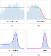 |
Fig. B.1 Classes of retrieved posterior distributions. The histogram gives the posterior distribution as found by the retrieval framework. The colored lines represent the best fit model for the posterior distribution, the black symbols below show how such a posterior will be represented in our data analysis plots. (a): unconstrained posterior (UC-type), (b): upper limit posterior (UL-type), (c): sensitivity limit posterior (SL-type), (d): constrained posterior (C-type). |
We determined the best fit model for each of the retrieved posterior distributions by fitting all four models. Thereafter, we used the log-likelihood function (Eq. (3), Sect. 2.2) to determine which model best described the retrieved posterior distribution. For the SL-type posterior, we required the maximum value of the fitted function was at least 1.3 times and maximally 10 times larger than the continuum probability at low abundances. If the peak probability was less than 1 .3 times the continuum value, we assumed a UL-type posterior. If the peak abundance was at least 10 times more probable than the low abundance continuum, we chose a C-type posterior instead. These cutoff values were chosen empirically to match what we would have obtained in a manual classification.
Appendix C Impact of randomized noise and additional species on retrieval results
As discussed in Sect. 2.3.1, we relied on two major assumptions in order to render our retrieval study computationally feasible and bias-free. First, we did not randomize the placement of the individual spectral points. Instead, we ran retrievals for the non-randomized spectral points and treated the LIFEsim noise as uncertainty on the spectrum. Second, our retrieval model did not allow for any additional gas species in the atmosphere. However, in real observations, we do not know what species are present. Therefore, it is important to investigate how robust these retrievals are with respect to false positive detections of molecules. There could be a finite probability of false positive detections, especially if combined with the randomized placement of the spectral points.
In this section, we investigate how randomizing spectral points and adding more species to the forward model impacts the performance of our retrieval routine at the proposed instrument requirements for LIFE (R = 50, S/N = 10, optimized noise scenario). To this purpose, we generated 20 different noise realizations of the spectrum at these requirements. We randomized the placement of each individual spectral point by randomly sampling a Gaussian distribution, where the standard deviation is determined by the wavelength dependent LIFEsim noise. Next, we ran a retrieval for every noise realization using the pyMultiNest settings outlined in Sect. 3. In addition to the molecules present in the input spectrum, we also retrieved for traces of NH3, PH3, and SO2. The resulting posteriors were then analyzed and classified using the method outlined in Appendix B.
We summarize our results in Figs. C.1, C.2, and C.3. Figure C.1 compares the MIR spectra corresponding to the posteriors retrieved from a single noise realization to the true spectrum. In Fig. C.2, we summarize all retrieved posterior types for the considered atmospheric gases. The leftmost column provides the retrieval findings for the nonrandomized input. Columns 1 to 20 list the results for the randomized input spectra. The rightmost column gives the percentage of retrievals on the randomized input that yielded the same posterior type as the nonrandomized retrieval. The last row provides the log-evidences ln(Z) for each retrieval run. In Fig. C.3, we show all retrieved posterior distributions as histograms and overlay them. Further, we plot the bin-wise mean and median of the posteriors obtained in the randomized retrievals and the posteriors found in the nonrandomized retrieval.
Appendix C.1 Truth versus spectra from noisy retrievals
 |
Fig. C.1 Fitted MIR emission spectra to a randomized input spectrum. The nonrandomized spectrum is marked by the black line, the randomized input for the retrieval are represented by red data points and error bars. The green shaded regions mark percentiles of the MIR spectra corresponding to the retrieved posteriors of the model parameters. |
As can be seen from Fig. C.1, our retrieval framework shows robust behavior even for randomized input spectra. The spectra corresponding to the retrieved posteriors roughly follow the true spectrum and generally do not significantly overfit to the noise. This observation holds for all noise realizations and is reinforced by the finding that the ln(Z) corresponding to the randomized retrievals are significantly smaller than in the nonrandomized case (see Fig. C.2). When overfitting, the retrieval models noise induced features accurately and thus the difference between the fitted spectrum and the input spectrum is small. This results in a ln(Z) value similar to the one obtained in retrievals of nonrandomized spectra. In our case, we are not fitting to the noise induced features. Thus, there is a larger difference between the fitted and input spectrum than in the nonrandomized case, which results in a smaller ln(Z).
Despite the good overall fit, a systematic offset between the true and the retrieved spectra starts to emerge above 10 µm. This offset becomes more pronounced at the longer wavelengths and results from the decreasing density of spectral points and increasing LIFEsim noise in this wavelength range. Between 10 and 12 µm, the molecules we consider have no strong absorption features and thus this range probes the planetary surface conditions. Offsets in this range will manifest themselves as shifts in the retrieved posteriors of P0, T0, and Rpl. Above 12 µm the shape of the MIR spectrum is dominated first by CO2 (up to ≈ 17 µm) and then by H2O features. Offsets from the truth in this range correspond to shifts in the retrieved abundance posteriors of these molecules. The described offsets are unique to each of the considered noise realizations and are diminished when averaging the retrieval results obtained from multiple noise realizations (see Sect. C.3 for a detailed discussion).
Appendix C.2 Robustness of the retrieved abundance posterior types
In this section, we take a closer look at the retrieved abundance posterior types to understand how robust different types are with respect to the noise randomization of the input spectrum. There are two underlying questions. First, we analyze how randomization affects the results for molecules that are present in the atmosphere. Second, we discuss if randomization can trigger false positive detections of molecules not present in the atmosphere.
From Fig. C.2, we see that the C-type posterior is robust under randomization. This means that, if retrieving the nonrandomized spectrum yields a C-type posterior, retrievals on noise realizations will mostly also yield C-type posteriors. This also shows in the high accuracy percentage. For our study, this observation implies that, at the determined LIFE requirements, we can expect to be capable of detecting CO2, H2O, and O3 in an Earth-twin atmosphere. We observe a similarly strong robustness for the UC-type posterior. From this, we can conclude that retrieval behavior for N2, O2, and CO is accurately predicted via the nonrandomized retrievals presented in our study.
Also, the UL-type posterior shows robust behavior with respect to noise randomization. Here we have to differentiate between two different scenarios: First, N2O, which is present in the input atmosphere and second, NH3, PH3, and SO2, which are not present.
For N2O, the high robustness of the UL-type posterior reassures our finding that N2O is likely not detectable in an Earth-twin at the proposed LIFE requirements. However, we do observe rare exceptions where an SL- or even a C-type posterior is retrieved. These exceptions correspond to cases where the randomization of the input spectrum results in a perceived amplification of the N2O absorption feature. This results in a detection of N2O. Naturally, the occurrence of a N2O detection is characterized by a strong overestimation of the retrieved N2O abundance. This can be seen from the retrieved posteriors of N2O displayed in Fig. C.3.
 |
Fig. C.2 Retrieved posterior types for atmospheric gases for the nonrandomized case (first column) and the 20 different noise realizations (columns 1 to 20). For posterior classification, we used the method outlined in Appendix B. The last row lists the Bayesian log-evidence ln(Z), the last column provides the retrieval accuracy (percentage of noise realizations resulting in the same posterior type as the centered case). |
For NH3, PH3, and SO2, we retrieve UL-type posteriors in all cases, which yields upper limits on the abundances of these molecules. We emphasize that retrieving a UL-type posterior is not a false positive detection. A UL-type posterior indicates that molecular abundances below the corresponding upper limit do not lead to an observable signature in the spectrum and therefore cannot be ruled out. The invariance of the retrieved UL-type posterior with respect to the different noise realizations indicates, that at LIFE requirements, we are robust to false positive detections of these molecules. We are aware that this analysis does not generally rule out false positive detections of arbitrary molecules. However, the fact that there was no false positive suggests that we are likely robust with respect to a large variety of false positives.
The most interesting case in this study is CH4. When not randomizing the input spectrum, we retrieve an SL-type posterior, which indicates that CH4 lies at the sensitivity limit (for the considered input data). When using the randomized spectra as input, the retrieved posterior types for CH4 vary between UL-, SL-, and C-type. Therefore, SL-type posteriors are not robust with respect to spectrum randomization. The observed variance in the retrieved posterior type originates because the randomization of input spectra can lead to an amplification or a reduction of the CH4 feature (similar as for N2O). Since the true CH4 abundance is close to the sensitivity limit, already small differences in the input spectrum can lead to differences in the retrieved posterior type. However, in contrast to N2O, the peaks of the retrieved SL-and U-type posteriors lie roughly within ±1 dex of the true CH4 abundance and do not have a tendency to overestimate it (see Fig. C.3). Still, the fact that the posterior type for CH4 depends on the noise realization leads us to the question of how we should interpret an SL-type posterior in a nonrandomized retrieval.
Appendix C.3 Interpretation of retrievals results for unrandomized spectra
As we discussed in the previous section, SL-type posteriors do not show robust behavior with respect to noise randomization. This observation raises the question of how to correctly interpret results obtained in retrievals of unrandomized input spectra. In Fig. C.3, we illustrate one possible answer to this question, which we further motivate in this section.
When considering the posteriors from the individual retrieval runs on randomized input spectra (gray shaded areas), we observe that in some cases there are non-neglectable differences between the different results. For the UC-type posteriors (N2,02, and CO) we observe only small differences between the individual retrieval runs. This underlines the robustness of this posterior type with respect to noise randomization. Similarly, for NH3, PH3, and SO2, we only observe little variance in the retrieved UL-type posteriors, which emphasizes the retrieval’s robustness with respect to false positive detections. Small differences between the different posteriors correspond to small biases in the retrieved upper abundance limits of these molecules. Similar conclusions can be drawn for N2O, where most of the retrieved posteriors are of the UL-type. The few deviances from the norm correspond to the previously described cases where an SL-type posterior that overestimates the abundance is retrieved.
 |
Fig. C.3 Retrieved normalized posterior distributions of model parameters for the 20 noise realizations. The posteriors of the individual noise realizations are plotted in light gray. The more posteriors overlap, the darker the gray becomes. The green dash-dotted line marks the mean, the blue dashed line the median of the posteriors for the different noise realizations. The posteriors found in the retrieval on the nonrandomized spectrum are plotted in solid red. The dotted line marks the true value for the Earth-twin atmosphere. Absence of the dotted line indicates that the species were not present in the atmosphere used to generate the input spectrum. |
The interpretation of posteriors is more subtle when considering C-type (Mpl, Rpl, P0, T0, CO2, H2O, and O3) or SL-type (CH4) posteriors. Here we observe a considerable variance in both the shape and the position of the individual posteriors. This observed variance in the posteriors is a bias that is evoked by the noise randomization of the input spectra. We further find that the variation occurs around the true value and its magnitude is comparable to the standard deviation of the posteriors obtained in the nonrandomized retrievals. Furthermore, we observe that the regions where many posteriors overlap (the dark regions) are similar in shape and position to the posteriors found in the unran-domized retrieval. In other words, the regions of parameter space that most retrievals agree on corresponds to the retrieval result obtained in the unrandomized retrieval.
Given the observations outlined above, the straightforward interpretation for retrieval results from unrandomized spectra is the following: the retrieved posterior distributions provide an estimate for the average retrieval behavior. Thus, if we take the average over the results from retrievals on different noise instances, it will converge toward the posterior distributions found in a retrieval on the unrandomized spectrum. To further motivate this interpretation, we plot the bin-wise mean and median of the posteriors retrieved from the 20 noise realizations in Fig. C.3. We find that already for 20 noise realizations, both mean and median are similar in shape and position to the posteriors from the unrandomized retrieval. For all cases, the median resembles the unrandomized case more closely because it is less sensitive to outliers.
In conclusion, this study suggests that retrieving on an unrandomized input spectrum eliminates biases that arise from noise randomization and will provide reliable estimates for the average behavior of the retrieval on randomized spectra. Generally, UC-, UL-, and C-type posteriors show robust behavior with respect to noise randomization. In contrast, SL-type posteriors are less robust and vary between C-, SL-, and UL-type in retrievals of randomized spectra. This variance in posterior type is closely linked to the fact that SL-type posteriors signify that an abundance is at the sensitivity limit of the retrieval for the studied spectral input. cloud-fee
Appendix D Retrieved parameter values
The retrieved parameter values are listed in Tables:
Table D.1: 3-20 µm, nominal case,
Table D.2: 3-20 µm, optimized case,
Table D.3: 4-18.5 µm, nominal case,
Table D.4: 4-18.5 µm, optimized case,
Table D.5: 6-17 µm, nominal case,
Table D.6: 6-17 µm, optimized case.
Retrieval results for the 3–20 µm wavelength range for the nominal case.
Retrieval results for the 3–20 µm wavelength range for the optimized case.
Retrieval results for the 4-18.5 µm wavelength range for the nominal case.
Retrieval results for the 4-18.5 µm wavelength range for the optimized case.
Retrieval results for the 6–17 µm wavelength range for the nominal case.
Retrieval results for the 6–17 µm wavelength range for the optimized case.
Appendix E Observation time estimates
Required observation time in days.
References
- Arney, G.N., Domagal-Goldman, S.D., & Meadows, V.S. 2018, AsBio, 18, 311 [NASA ADS] [Google Scholar]
- Barstow, J.K., & Heng, K. 2020, SSR, 216, 82 [NASA ADS] [Google Scholar]
- Barstow, J.K., Changeat, Q., Garland, R., et al. 2020, MNRAS, 493, 4884-909 [NASA ADS] [CrossRef] [Google Scholar]
- Brandt, T.D., & Spiegel, D.S. 2014, Proc. Natl. Acad. Sci. U.S.A., 111, 13278 [NASA ADS] [CrossRef] [Google Scholar]
- Bryson, S., Kunimoto, M., Kopparapu, R.K., et al. 2021, AJ, 161, 36 [NASA ADS] [CrossRef] [Google Scholar]
- Buchner, J., Georgakakis, A., Nandra, K., et al. 2014, A&A, 564, A125 [NASA ADS] [CrossRef] [EDP Sciences] [Google Scholar]
- Carnall, A.C. 2017, ArXiv e-prints [arXiv:1705.05165] [Google Scholar]
- Carriön-Gonzalez, Ö., Garcia Munoz, A., Cabrera, J., et al. 2020, A&A, 640, A136 [NASA ADS] [CrossRef] [EDP Sciences] [Google Scholar]
- Catling, D.C., Krissansen-Totton, J., Kiang, N.Y., et al. 2018, Astrobiology, 18, 709 [NASA ADS] [CrossRef] [Google Scholar]
- Chen, J., & Kipping, D. 2016, ApJ, 834, 17 [Google Scholar]
- Chubb, K.L., Rocchetto, M., Yurchenko, S.N., et al. 2021, A&A, 646, A21 [NASA ADS] [CrossRef] [EDP Sciences] [Google Scholar]
- Cockell, C., Léger, A., Fridlund, M., et al. 2009, Astrobiology, 9, 1, pMID: 19203238 [NASA ADS] [CrossRef] [Google Scholar]
- Dannert, F., Ottiger, M., Quanz, S.P., et al. 2022, A&A, 664, A22 (Paper II) [NASA ADS] [CrossRef] [EDP Sciences] [Google Scholar]
- Deming, D., Louie, D., & Sheets, H. 2018, PASP, 131, 013001 [Google Scholar]
- Des Marais, D.J., Harwit, M.O., Jucks, K.W., et al. 2002, Astrobiology, 2, 153 [NASA ADS] [CrossRef] [Google Scholar]
- Ertel, S., Defrère, D., Hinz, P., et al. 2020, AJ, 159, 177 [Google Scholar]
- Fauchez, T.J., Turbet, M., Villanueva, G.L., et al. 2019, ApJ, 887, 194 [NASA ADS] [CrossRef] [Google Scholar]
- Feng, Y.K., Line, M.R., Fortney, J.J., et al. 2016, ApJ, 829, 52 [NASA ADS] [CrossRef] [Google Scholar]
- Feng, Y.K., Robinson, T.D., Fortney, J.J., et al. 2018, AJ, 155, 200 [NASA ADS] [CrossRef] [Google Scholar]
- Feroz, F., Hobson, M.P., & Bridges, M. 2009, MNRAS, 398, 1601-14 [NASA ADS] [CrossRef] [Google Scholar]
- Feroz, F., Hobson, M., Cameron, E., & Pettitt, A. 2013, Open J. Astrophys., 2 [Google Scholar]
- Fu, Q., & Liou, K.N. 1992, J. Atmos. Sci., 49, 2139 [NASA ADS] [CrossRef] [Google Scholar]
- Gaudi, B.S., Seager, S., Mennesson, B., et al. 2020, ArXiv e-prints [arXiv:2001.06683] [Google Scholar]
- Goody, R., West, R., Chen, L., & Crisp, D. 1989, J. Quant. Spectr. Rad. Transf., 42, 539 [NASA ADS] [CrossRef] [Google Scholar]
- Guillot, T. 2010, A&A, 520, A27 [NASA ADS] [CrossRef] [EDP Sciences] [Google Scholar]
- Harman, C.E., & Domagal-Goldman, S. 2018, Biosignature False Positives, eds. H.J. Deeg, & J.A. Belmonte, 71 [Google Scholar]
- Hastings, W.K. 1970, Biometrika, 57, 97 [NASA ADS] [CrossRef] [Google Scholar]
- Hatzes, A.P., & Rauer, H. 2015, ApJ, 810, L25 [NASA ADS] [CrossRef] [Google Scholar]
- Jeffreys, H. 1998, The Theory of Probability (Oxford Classic Texts in the Physical Sciences (OUP Oxford), 432 [Google Scholar]
- Kawashima, Y., & Rugheimer, S. 2019, ApJ, 157, 213 [CrossRef] [Google Scholar]
- Kitzmann, D., Patzer, A.B.C., von Paris, P., Godolt, M., & Rauer, H. 2011, A&A, 531, A62 [NASA ADS] [CrossRef] [EDP Sciences] [Google Scholar]
- Komacek, T.D., Fauchez, T.J., Wolf, E.T., & Abbot, D.S. 2020, ApJ, 888, L20 [NASA ADS] [CrossRef] [Google Scholar]
- Lacis, A.A., & Oinas, V. 1991, J. Geophys. Res.: Atmos., 96, 9027 [NASA ADS] [CrossRef] [Google Scholar]
- Lavvas, P., Koskinen, T., Steinrueck, M.E., Munoz, A.G., & Showman, A.P. 2019, ApJ, 878, 118 [NASA ADS] [CrossRef] [Google Scholar]
- Lederberg, J. 1965, Nature, 207, 9 [NASA ADS] [CrossRef] [Google Scholar]
- Léger, A., Mariotti, J.M., Mennesson, B., et al. 1996, Icarus, 123, 249 [CrossRef] [Google Scholar]
- Léger, A., Defrère, D., Garcia Munoz, A., et al. 2019, Astrobiology, 19, 797 [CrossRef] [Google Scholar]
- Line, M., Quanz, S.P., Schwieterman, E.W., et al. 2019, BAAS, 51, 271 [NASA ADS] [Google Scholar]
- Lippincott, E.R., Eck, R.V., Dayhoff, M.O., & Sagan, C. 1967, ApJ, 147, 753 [NASA ADS] [CrossRef] [Google Scholar]
- Lovelock, J.E. 1965, Nature, 207, 568 [NASA ADS] [CrossRef] [Google Scholar]
- Madhusudhan, N. 2018, Handbook of Exoplanets, 2153 [CrossRef] [Google Scholar]
- Madhusudhan, N., & Seager, S. 2009, ApJ, 707, 24 [NASA ADS] [CrossRef] [Google Scholar]
- Mayor, M., & Queloz, D. 1995, Nature, 378, 355 [Google Scholar]
- Meadows, V.S., Reinhard, C.T., Arney, G.N., et al. 2018, Astrobiology, 18, 630 [NASA ADS] [CrossRef] [Google Scholar]
- Metropolis, N., Rosenbluth, A.W., Rosenbluth, M.N., Teller, A.H., & Teller, E. 1953, J. Chem. Phys., 21, 1087 [CrossRef] [Google Scholar]
- Mettler, J.-N., Quanz, S.P., & Helled, R. 2020, AJ, 160, 246 [NASA ADS] [CrossRef] [Google Scholar]
- Mollière, P., Boekel, R.V., Dullemond, C., Henning, T., & Mordasini, C. 2015, ApJ, 813, 47 [CrossRef] [Google Scholar]
- Mollière, P., Wardenier, J.P., van Boekel, R., et al. 2019, A&A, 627, A67 [NASA ADS] [CrossRef] [EDP Sciences] [Google Scholar]
- Mollière, P., Stolker, T., Lacour, S., et al. 2020, A&A, 640, A131 [Google Scholar]
- Mueller-Wodarg, I.C.F., Strobel, D.F., Moses, J.I., et al. 2008, Neutral Atmospheres, eds. A.F. Nagy, A. Balogh, T.E. Cravens, M. Mendillo, & I. Mueller-Wodarg (New York: Springer New York), 191 [Google Scholar]
- Otegi, J.F., Bouchy, F., & Helled, R. 2020, A&A, 634, A43 [NASA ADS] [CrossRef] [EDP Sciences] [Google Scholar]
- Peterson, B.M., Fischer, D., & LUVOIR Science and Technology Definition Team. 2017, AAS, 229, 405.04 [Google Scholar]
- Quanz, S.P., Kammerer, J., Defrère, D., et al. 2018, SPIE Conf. Ser., 10701, 107011I [NASA ADS] [Google Scholar]
- Quanz, S.P., Absil, O., Angerhausen, D., et al. 2021, ArXiv e-prints [arXiv:1908.01316] [Google Scholar]
- Quanz, S.P., Ottiger, M., Fontanet, E., et al. 2022, A&A, 664, A21 (Paper I) [NASA ADS] [CrossRef] [EDP Sciences] [Google Scholar]
- Robinson, T.D. 2011, ApJ, 741, 51 [NASA ADS] [CrossRef] [Google Scholar]
- Robinson, T.D., Meadows, V.S., & Crisp, D. 2010, ApJ, 721, L67 [NASA ADS] [CrossRef] [Google Scholar]
- Rothman, L.S., Wattson, R.B., Gamache, R., Schroeder, J.W., & McCann, A. 1995, in Atmospheric Propagation and Remote Sensing IV, ed. J.C. Dainty, 2471, International Society for Optics and Photonics (SPIE), 105, 111 [Google Scholar]
- Rothman, L., Gordon, I., Barber, R., et al. 2010, J. Quant. Spectr. Rad. Transf., 111, 2139, xVIth Symposium on High Resolution Molecular Spectroscopy (HighRus-2009) [NASA ADS] [CrossRef] [Google Scholar]
- Rothman, L.S., Gordon, I.E., Babikov, Y., et al. 2013, J. Quant. Spec. Rad. Transf., 130, 4 [NASA ADS] [CrossRef] [Google Scholar]
- Rugheimer, S., Kaltenegger, L., Zsom, A., Segura, A., & Sasselov, D. 2013, Astrobiology, 13, 251 [NASA ADS] [CrossRef] [Google Scholar]
- Rugheimer, S., Segura, A., Kaltenegger, L., & Sasselov, D. 2015, ApJ, 806, 137 [NASA ADS] [CrossRef] [Google Scholar]
- Schwieterman, E.W. 2018, Handbook of Exoplanets, 3173 [CrossRef] [Google Scholar]
- Schwieterman, E.W., Kiang, N.Y., Parenteau, M.N., et al. 2018, Astrobiology, 18, 663 [CrossRef] [Google Scholar]
- Schwieterman, E.W., Robinson, T.D., Meadows, V.S., Misra, A., & Domagal-Goldman, S. 2015, ApJ, 810, 57 [NASA ADS] [CrossRef] [Google Scholar]
- Seager, S., Turner, E., Schafer, J., & Ford, E. 2005, Astrobiology, 5, 372 [NASA ADS] [CrossRef] [Google Scholar]
- Seager, S., Bains, W., & Petkowski, J. 2016, Astrobiology, 16, 465 [NASA ADS] [CrossRef] [Google Scholar]
- Selsis, F., Despois, D., & Parisot, J.P. 2002, A&A, 388, 985 [NASA ADS] [CrossRef] [EDP Sciences] [Google Scholar]
- Sing, D.K., Fortney, J.J., Nikolov, N., et al. 2016, Nature, 529, 59 [NASA ADS] [CrossRef] [Google Scholar]
- Skilling, J. 2006, Bayesian Anal., 1, 833 [Google Scholar]
- Tennyson, J., Yurchenko, S.N., Al-Refaie, A.F., et al. 2016, J. Mol. Spectro., 327, 73 [NASA ADS] [CrossRef] [Google Scholar]
- Trotta, R. 2017, Bayesian Methods in Cosmology [Google Scholar]
- van de Schoot, R., Depaoli, S., King, R., et al. 2021, Nat. Rev. Methods Primers, 1, 3 [CrossRef] [Google Scholar]
- von Paris, P., Hedelt, P., Selsis, F., Schreier, F., & Trautmann, T. 2013, A&A, 551, A120 [NASA ADS] [CrossRef] [EDP Sciences] [Google Scholar]
- Wolfgang, A., Rogers, L.A., & Ford, E.B. 2016, ApJ, 825, 19 [NASA ADS] [CrossRef] [Google Scholar]
- Wunderlich, F., Scheucher, M., Grenfell, J.L., et al. 2021, A&A, 647, A48 [NASA ADS] [CrossRef] [EDP Sciences] [Google Scholar]
- Yurchenko, S.N., Mellor, T.M., Freedman, R.S., & Tennyson, J. 2020, MNRAS, 496, 5282 [NASA ADS] [CrossRef] [Google Scholar]
- Zahnle, K., Haberle, R.M., Catling, D.C., & Kasting, J.F. 2008, J. Geophys. Res.: Planets, 113 [Google Scholar]
- Zeng, L., Sasselov, D.D., & Jacobsen, S.B. 2016, ApJ, 819, 127 [NASA ADS] [CrossRef] [Google Scholar]
However, clouds can also increase the reflectivity and signal for molecules such as molecular oxygen (O2) that are well-mixed in the atmosphere of a terrestrial planet (Kawashima & Rugheimer 2019).
According to the brightness distribution of exozodi disks used in recent LIFE detection yield estimate (Quanz et al. 2022), which is based on the results from the HOSTS survey (Ertel et al. 2020), <20% of the disks show such low emission.
All Tables
Parameters used in the retrievals, their input values, prior distributions, and the validation results.
All Figures
|
Fig. 1 Schematic illustrating our atmospheric retrieval framework. |
| In the text | |
|
Fig. 2 Comparison of the Earth-twin MIR emission spectra calculated with various different models. We plot the photon flux received from an Earth-twin located 10 pc from the sun. The solid blue line is the MIR thermal emission calculated with petitRADTRANS using the settings discussed in Sect. 2.3.1. The blue-shaded region indicates the most optimistic LIFEsim uncertainty (S/N = 20) used in our retrievals. The red dashed line represents a cloud-free Earth model by Daniel Kitzmann (priv. comm.), which takes scattering into account. The green and black dashed-dotted lines are the cloudy (60% cloud coverage) and cloud-free modern Earth spectra from Rugheimer et al. (2015) that account for scattering. |
| In the text | |
|
Fig. 3 Wavelength dependence of different opacity sources. Upper panel: the opacity of a cloudless Earth-twin atmosphere as a function of wavelength. Gray shading shows the amount of light blocked by the atmosphere. Lower panel: contribution of the different molecules to the opacity of the Earth-twin atmosphere as a function of wavelength. Dark regions indicate a high opacity, as is indicated by the colorbar. |
| In the text | |
|
Fig. 4 Results from the validation run outlined in Sect. 3. (a) Corner plot for the posterior distributions of the planetary surface temperature T0, surface pressure P0, radius Rpl, mass Mpl, and retrieved abundances of different molecules. The red lines indicate the values used to generate the input spectrum. Additionally, we plot the retrieved median and the 16th and 84th percentile as dashed lines in every posterior plot. (b) Retrieved P−T profile. The shaded green regions show the uncertainties on the retrieved profile. In the bottom left corner of the P−T profile plot, we display P0 and T0. The red cross marks the input values. (c) The retrieved emission spectrum Fretrieved relative to the input emission spectrum for the retrieval Finput. |
| In the text | |
|
Fig. 5 Ratio between the wavelength-dependent S/N of the optimized case and the nominal case. This ratio is independent of the overall S/N and the R of the Spectrum. |
| In the text | |
|
Fig. 6 Examples of input spectra used in the grid retrievals for the nominal case (left: the lowest quality input with R = 20, S/N = 5; right: the highest quality input with R = 100, S/N = 20). In gray, we provide the full resolution petitRADTRANS Earth spectrum. The red step function represents the wavelength-binning of the input data. Further, the blue shaded region represents the uncertainty for the corresponding bin. We also mark the absorption features of the considered atmospheric gases. |
| In the text | |
|
Fig. 7 Retrieved exoplanet parameters for the different grid points for the wavelength range 3–20 μm in the nominal case. Here, Mpl is the mass, Rpl the radius, P0 the surface pressure, and T0 the surface temperature of the exoplanet. The error bars denote the 68% confidence intervals. For Mpl and Rpl, we also plot the assumed prior distributions. For T0 and P0, we assumed flat, broad priors. The vertical lines mark the true parameter values. |
| In the text | |
|
Fig. 8 Retrieved mass mixing ratios of the different trace gases present in Earth’s atmosphere for an input spectrum wavelength range of 3–20 μm in the nominal case. The vertical lines mark the true abundances whereas the shaded regions mark the ± 0.5 dex, ±1.0 dex, and ±1.5 dex regions. |
| In the text | |
 |
Fig. 9 As for Fig. 8 but for retrieved abundances relative to CO2. |
| In the text | |
|
Fig. 10 Wavelength-dependent posterior types retrieved for the different trace gases in the nominal case (a)–(c) and the optimized case (d)–(f). The lowermost panel gives the color coding for the different posterior types. The abbreviations used for the different posteriors are introduced in Sect. 4.2. (a, d): 3–20 μm, (b, e): 4–18.5 μm, (c,f): 6–17 μm. |
| In the text | |
|
Fig. 11 Performance comparison between different retrieval studies. The error bars correspond to the 68% confidence intervals of the retrieved posterior distributions. The emitted light study from this work for (R = 50, S/N = 10 (green downward triangle) and R = 35, S/N = 15 (orange upward triangle), 3–20 μm in the optimized case); the reflected light study by Feng et al. (2018) (R = 70, S/N=10 (blue dot), R = 70, S/N = 15 (red square), 0.4–1.0 μm). |
| In the text | |
|
Fig. A.1 Results from the P–T model retrievals. The first row displays the log-evidence ln(Z) of the different models. The second row shows a zoomed in view of the high log-evidence region of the first row to allow for better comparison. The bottom row displays the retrieved best fit P–T profiles for the fourth order polynomial, the Madhusudhan & Seager (2009) model, and the two Guillot models (Guillot 2010; Mollière et al. 2019). The data for the true P–T profiles is taken from Fig. 1 in Mueller-Wodarg et al. (2008). |
| In the text | |
|
Fig. B.1 Classes of retrieved posterior distributions. The histogram gives the posterior distribution as found by the retrieval framework. The colored lines represent the best fit model for the posterior distribution, the black symbols below show how such a posterior will be represented in our data analysis plots. (a): unconstrained posterior (UC-type), (b): upper limit posterior (UL-type), (c): sensitivity limit posterior (SL-type), (d): constrained posterior (C-type). |
| In the text | |
|
Fig. C.1 Fitted MIR emission spectra to a randomized input spectrum. The nonrandomized spectrum is marked by the black line, the randomized input for the retrieval are represented by red data points and error bars. The green shaded regions mark percentiles of the MIR spectra corresponding to the retrieved posteriors of the model parameters. |
| In the text | |
|
Fig. C.2 Retrieved posterior types for atmospheric gases for the nonrandomized case (first column) and the 20 different noise realizations (columns 1 to 20). For posterior classification, we used the method outlined in Appendix B. The last row lists the Bayesian log-evidence ln(Z), the last column provides the retrieval accuracy (percentage of noise realizations resulting in the same posterior type as the centered case). |
| In the text | |
|
Fig. C.3 Retrieved normalized posterior distributions of model parameters for the 20 noise realizations. The posteriors of the individual noise realizations are plotted in light gray. The more posteriors overlap, the darker the gray becomes. The green dash-dotted line marks the mean, the blue dashed line the median of the posteriors for the different noise realizations. The posteriors found in the retrieval on the nonrandomized spectrum are plotted in solid red. The dotted line marks the true value for the Earth-twin atmosphere. Absence of the dotted line indicates that the species were not present in the atmosphere used to generate the input spectrum. |
| In the text | |
Current usage metrics show cumulative count of Article Views (full-text article views including HTML views, PDF and ePub downloads, according to the available data) and Abstracts Views on Vision4Press platform.
Data correspond to usage on the plateform after 2015. The current usage metrics is available 48-96 hours after online publication and is updated daily on week days.
Initial download of the metrics may take a while.