| Issue |
A&A
Volume 689, September 2024
|
|
|---|---|---|
| Article Number | A38 | |
| Number of page(s) | 10 | |
| Section | Interstellar and circumstellar matter | |
| DOI | https://doi.org/10.1051/0004-6361/202450297 | |
| Published online | 29 August 2024 | |
Volume density maps of the 862 nm DIB carrier and interstellar dust
Hints on the role of carbon-rich ejecta from AGB stars★
1
ACRI-ST, Centre d’Etudes et de Recherche de Grasse (CERGA),
10 Av. Nicolas Copernic,
06130
Grasse, France
e-mail: nick.cox@acri-st.fr
2
ACRI-ST,
260 Route du Pin Montard,
Sophia-Antipolis, France
3
GEPI, Observatoire de Paris, Université PSL, CNRS,
5 place Jules Janssen,
92195
Meudon, France
Received:
9
April
2024
Accepted:
2
June
2024
Context. The carbonaceous macromolecules imprinting the numerous absorptions called diffuse interstellar bands (DIBs) in astronomical spectra are omnipresent in the Galaxy and beyond. They represent a considerable reservoir of organic matter. However, their chemical formulae, formation, and destruction sites remain unknown. Their spatial distribution and the local relation to other interstellar species is key to tracing their role in the lifecycle of organic matter.
Aims. Volume density maps bring local instead of line-of-sight distributed information and allow for new diagnostics to be captured. We present the first large-scale volume (3D) density map of a DIB carrier and compare it with an equivalent map of interstellar dust.
Methods. The DIB carrier map was obtained through hierarchical inversion of ~202 000 measurements of the 8621 nm DIB obtained with the Gaia-RVS instrument. It covers about 4000 pc around the Sun in the Galactic plane. We built a dedicated interstellar dust map based on the extinction towards the same target stars.
Results. At the ≃50 pc resolution of the maps, the shape of the 3D DIB distribution is found to be remarkably similar to the 3D distribution of dust. On the other hand, the DIB-to-dust local density ratio increases in low-dust areas. It is also increasing away from the disk, however, the minimum ratio is found to be shifted above the Galactic plane to Z=≃+50pc. Finally, the average ratio is also surprisingly found to increase away from the Galactic Center. We suggest that the three latter trends may be indications of a dominant contribution of material from the carbon-rich category of dying giant stars to the formation of the carriers. Our suggestion is based on recent catalogs of asymptotic giant branch (AGB) stars and estimates of the mass fluxes of their C-rich and O-rich ejecta.
Key words: stars: AGB and post-AGB / ISM: clouds / dust, extinction / evolution / ISM: lines and bands / ISM: structure
The DIB and extinction 3D maps are available at the CDS via anonymous ftp to cdsarc.cds.unistra.fr (130.79.128.5) or via https://cdsarc.cds.unistra.fr/viz-bin/cat/J/A+A/689/A38
© The Authors 2024
 Open Access article, published by EDP Sciences, under the terms of the Creative Commons Attribution License (https://creativecommons.org/licenses/by/4.0), which permits unrestricted use, distribution, and reproduction in any medium, provided the original work is properly cited.
This article is published in open access under the Subscribe to Open model. Subscribe to A&A to support open access publication.
1 Introduction
Diffuse interstellar bands (DIBs) consist of absorptions of various shapes and depths distributed in the optical and near-infrared spectra of distant objects. Catalogues of DIBs have been consistently expanding due to the accumulation of stellar spectra of rising quality, reaching more than 500 different features (see Fan et al. 2019 and references therein). These bands are omnipresent in the Universe, detected in both the local Galaxy as well as in neighbouring and distant galaxies (Heckman & Lehnert 2000; Cordiner et al. 2011; Monreal-Ibero et al. 2015). The column densities of their carriers (i.e., the absorbing species), measured through the fraction of absorbed light, are known to be correlated (to a varying extent) with the amount of interstellar dust or gas (Vos et al. 2011; Friedman et al. 2011), making them potential proxies for the columns of foreground interstellar matter (Phillips et al. 2013). A detailed analysis of the band spectral profiles reveals structures that are indicative of rotating large molecules (Sarre et al. 1995) whose presence in the interstellar medium (ISM) is also known from their infrared signatures arising from different stretching or vibration modes of polycyclic aromatic hydrocarbons (PAHs, Leger & D’Hendecourt 1985). Despite progress in laboratory astrophysics, their carriers have effectively remained unidentified (Cami & Cox 2014), with the exception of only four bands, situated in the near-infrared part of the spectrum which have been assigned to the ionized buckmin-sterfullerene, C60+ (Foing & Ehrenfreund 1994; Campbell et al. 2015; Cordiner et al. 2019).
Adding to the mystery of their composition (and despite all measurements taken thus far) there is no consensus on their formation sites and processes, nor the way they are destroyed or transformed. The main reason is the poor diagnostic on the location of the carrier provided by individual absorption measurements; indeed, the location can be anywhere between the Sun and the observed target star. This is why, besides the identification of carriers that would undoubtedly be an important discovery in terms of understanding the chemical complexity and composition of organic matter in space, constraining their spatial distribution is equally important. It will shed light on their formation and destruction sites and, in turn, on the processes at play and the effects of local physical conditions. Once we know the constraints on their formation and lifetimes, even without identifying them, DIBs can be used as probes of the physico-chemical conditions of the interstellar medium, not only in the local galaxy, but also further away in distant galaxies. This will enable unique diagnostics to be undertaken.
Globally, all DIBs are found to be positively correlated with the amount of dust and total gas columns. However, there is a large scatter on these relations and the dependence on molecular hydrogen columns may be negative, suggesting environmental conditions play a fundamental role in the relative abundance of the carriers (e.g. Friedman et al. 2011). Indeed, according to the most detailed studies of nearby dense clouds, the strongest DIBs appear to respond differently to changes in the local physical conditions of ISM (Fan et al. 2019; Vos et al. 2011; Friedman et al. 2011). In particular, the local effective radiation field is affecting the relative abundances between different DIB carriers (Vos et al. 2011). Also, most DIB carriers become depleted in opaque regions, namely, towards the interior of dense interstellar clouds. This effect has been known for a long time (Snow & Cohen 1974) and has now been quantitatively documented in various ways (Lan et al. 2015; Fan et al. 2017; Elyajouri et al. 2017). Furthermore, the ratio between DIB carrier column and reddening starts to decrease for lines of sight crossing the more central regions of dense clouds, at an average reddening of E(B – V) = 0.5–1.0 mag (Lan et al. 2015) or at an average molecular fraction of 0.3 (Fan et al. 2017). This is called the “skin effect.” However, other factors are also at play, as suggested from the principle-component analysis presented by Ensor et al. (2017).
The 862 nm DIB is a broad band (FWHM of ~0.4 nm), whose relatively small depth makes it challenging to measure in the spectra of cool stars. However, being spectrally close to ionized calcium lines commonly used to constrain the stellar parameters, its study benefits from stellar spectroscopic surveys using these stellar lines. Consequently, its properties have been well studied, especially thanks to the ground-based stellar spectroscopic survey RAVE (Kos et al. 2013). They have been found to be similar to the majority of bands, and the correlation between the 862 nm DIB and interstellar reddening (or visual extinction) has been found to be relatively tight (Kos et al. 2013, 2014; Puspitarini et al. 2015). The measurements did not yet allow for the detection of the depletion in very opaque regions. Its study was recently boosted due to its presence in the spectral interval selected for the Radial Velocity Spectrometer (RVS), the high-resolution spectrometer on board Gaia. With Gaia, DIB measurements could be coupled with high precision parallaxes of target stars (Gaia Collaboration 2016; Gaia Collaboration 2023c). Gaia Collaboration (2023b) presented individual DIB measurements from Gaia Data Release 3 for 476 000 stars based on a comparison of observed spectra with stellar models and explored the relationship with the extinction and the target location.
Maps of DIB equivalent widths (EWs) or absorption strengths (quantities proportional to integrated DIB carrier density columns) have been presented for several DIBs based on ground surveys (Kos et al. 2014; Baron et al. 2015; Zasowski et al. 2015) and more recently on Gaia data (Gaia Collaboration 2023b; Gaia Collaboration 2023a). They display, for each location in space, the measured cumulative value of DIB carriers, integrated between the Sun and the target star. All these pseudo-3D maps revealed a similarity with the reddening, but there are some apparently contradictory results. Based on integrated line-of-sight values of the 862 nm DIB observed with RAVE, Kos et al. (2014) found a DIB scale height above the Galactic disk of about 200 pc, far above the dust scale height of about 100 pc, while Gaia Collaboration (2023b) derived for the same DIB and from Gaia data a scale height similar to the one of dust. More precisely, using full-sky Gaia data, the authors found evidence for a significant variability of the scale height according to the Galactic area. They attributed the difference with respect to the RAVE result to the use of different longitude and latitude ranges for the two studies.
At variance with mapping of Sun-star integrated quantities, full 3D tomography is aimed at computing the local volume density of a species at each point in space. A 3D mapping of the strong 578 nm DIB has been presented by Farhang et al. (2019) for the so-called Local Bubble, a 250 pc wide region around the Sun, based on 360 lines of sight. Nowadays, Milky Way large-scale full 3D maps have been constructed solely for interstellar dust, using extinction and color excess measurements of Galactic target stars. To do so, differentials of the cumulative data along radial directions (Chen et al. 2019; Green et al. 2019) or full 3D inversion techniques (Vergely et al. 2001; Leike et al. 2020; Rezaei Kh. et al. 2020) were applied to a whole set of integrated data. Over the last years, 3D extinction maps have been constantly improved, following the accurate parallaxes and photometric data from Gaia (Lallement et al. 2022; Vergely et al. 2022). Here, we build the first, large-scale, fully 3D map of a DIB carrier, tracing it out to ~2000 pc from the Sun, and do the first comparisons between local values of DIB carriers and dust grains. The data are presented in Sect. 2 and the methodology in Sect. 3. The results are presented in Sect. 4 and discussed in Sect. 5.
2 Data
This study takes as input the Gaia DR3 data release (Gaia Collaboration 2016; Gaia Collaboration 2023c), which includes DIB measurements for 463 486 sources, constituting the largest all-sky survey of DIBs to date (Gaia Collaboration 2023b). The reported DIB equivalent width values are integrated line-of-sight measurements.
The following procedure, considering the recommendations from Gaia Collaboration (2023b), has been defined to prepare a high-fidelity input catalog for inversion. We selected all (463 486) objects with reported DIB equivalent widths in Gaia DR3. Among them, we selected all objects that have a parallax error <20% (ePlx/Plx < 0.2), a DIB quality flag = 0, 1, or 2 (qDIB < 3), |z| < 400 pc (only sources within 400 pc of the galactic plane), r < 5000 pc (only sources within 5 kpc of the Sun). This produces an input catalog of 202 340 sources. We further investigated whether additional filtering benefits the reconstruction. Saydjari et al. (2023) argued that residual stellar lines not considered by the Gaia processing pipeline have mistakenly been fitted as DIBs. The authors produced a catalog of cleaned measurements based on their own analysis of publicly available RVS spectra; however, due to the limited number of such public data, this catalog is not large enough to be used for inversion. We attempted to exclude features at 861.6, 861.7, and 862.5 nm which are thought to be stellar lines masquerading as DIBs. We note that λDIB is measured in the stellar rest frame, to which real DIBs would not be expected to align. Therefore, to remove the most obvious stellar line contamination, we applied the following filtering on λDIB (in nm): 862.52 < λDIB < 862.58, 861.76 < λDIB < 861.78, 861.66 < λDIB < 861.70. This reduces the input catalog size to 175 578 sources. However, the effect of this filtering (tested also with applying variations on the exact lambda boundaries) on the map reconstruction turned out to be negligible. Another effect we noticed in the input catalog is that the relation between DIB strength and distance changes with the effective temperature of the background star for targets at small distances. This suggests a systematic uncertainty in the measurement of the DIB strength that is most noticeable at shortest distances, where the DIBs are weakest. Since it essentially affects the distribution very close to the Sun, we did not remove those targets.
Finally, additional filtering could also be applied to the DIB EW uncertainty (eEWDIB). We considered a filtering on eEWDIB/EWDIB <0.3, but it removes too much data, particularly for the low EW values (the input catalog is reduced to 122,585 sources).
In fact, the reconstruction algorithm manages errors and outliers in a robust way. In the tomography steps, we did not use individual DIB equivalent widths, but an average of many values made over spatial boxes. The size of the boxes depends on the resolution. For a 100-pc resolution reconstruction, boxes have a size of 100 × 100 × 100 pc. The algorithm averages each DIB equivalent width by 1/eEWDIB2. During the inversion, the average EWDIB is used in each box together with an estimation of the error of the average in the box. The error in each box is computed from the standard deviation of the individual EWDIBs present in the box. Incorrect EWDIB values in a box will lead to an increase of the standard deviation and the data (average over the box) will have lower weight in the result. Thus, pre-filtering on eEWDIB does not significantly alter (improve) the results. Similarly, the algorithm is robust against biases related to the effective temperature of the background stars. Following the adage of “less is more,” the simpler source filter (“step 2” above) was finally adopted.
3 Methodology
3.1 Tridimensional (3D) tomography
The reconstruction of the volume (3D) density of either interstellar dust grains producing the extinction or of DIB carriers is based on the inversion of a catalog of measured integrated values, that is, as seen from the origin up to a given point (x, y, z) at a distance, d, the target star location. The integrated quantity is the stellar light extinction in the first case, and the absorption equivalent width in the second. However, this catalog is made up of a limited and irregular sampling of locations in 3D space. Moreover, the accuracy of this reconstruction is limited by the accuracy of the distance, d, the uncertainty on the measured quantity, the sampling density, and the choice of the prior distribution. As a result, the spatial resolution and quality of the final density maps derived through inversion depends in large part on the number of data points, and their accuracy, which sample the true 3D distribution. Increasing the number of data points will improve the retrieval of spatial information, particularly in the radial direction. On the other hand, allowing for the inclusion of inaccurate data points will lead to the appearance of false features. Consequently, filtering applied in Sect. 2 is essential.
We applied to the selected data (cf. Sect. 2) the same hierarchical, iterative inversion technique used in Lallement et al. (2022) and Vergely et al. (2022) for the dust extinction. According to this technique, the achievable spatial resolution of the map is variable in 3D space and governed by the target star density at each location. At each iteration, the maximum resolution (or minimum correlation length imposed to regularize the inversion) was increased and the solution was improved (where possible). It was also kept similar to the solution of the previous iteration at locations where there are not enough targets. Here, due to the limited spatial density of the targets and their inhomogeneous distribution in 3D space, the minimum correlation length was 50 pc, much larger than the one achievable for dust (for the latter, the available input catalog of extinction and distance is an order of magnitude larger).
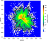 |
Fig. 1 Coverage of sources in the input catalog along the Galactic plane. The number of sources per 1003 pc3 cell is color-coded. All sources with abs(z) <50 pc are included. The limit of five targets per cell used in the statistical study is marked by a thick black line. |
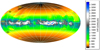 |
Fig. 2 Aitoff projection of the maximum reliable distance map for the DIB 3d reconstruction. Iso-Galactic longitudes and latitudes are drawn spaced by 30°. The Galactic Center (l = 0) is at the center and longitudes are increasing to the left. The reconstruction in the Galactic plane (|b| < 15°) has the highest fidelity. |
3.2 Limits of the multi-scale Bayesian inversion of the DIB equivalent widths
Figure 1 shows the coverage (source density) of the input catalog in the Galactic plane (all sources with abs(z) < 50 pc are shown). The vertical scale upper limit is set such that all bins with at least five input sources are highlighted.
Beyond 2–3 kpc there are fewer objects (the exact value depending on the longitude and latitude), while the sampled volume increases exponentially. Including a margin, the reconstructed density cubes are cut off at 4 kpc. To quantify the fidelity of the 3D maps we also computed a “maximum reliable distance” map. We set the limiting distance to the distance of the most distant distance bin with at least five stars. Beyond this bin, the accuracy of the map was severely hampered by the lack of input data. The maximum reliable distance map (as a function of galactic longitude and latitude) for the DIB reconstruction is shown in Fig. 2 and it is crucial for interpreting the 3D distribution of DIBs at the furthest distances. The DIB densities near or beyond this distance are inaccurate and should be interpreted or applied with great caution.
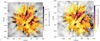 |
Fig. 3 862.1 nm DIB carrier volume density (left) and extinction volume density (right) in the plane parallel to the Galactic plane and containing the Sun. Coordinates are in parsec from the Sun location. The Galactic Center is to the right and the longitude increases anti-clockwise. Dashed lines are iso-galactocentric distances spaced by 1000 pc. The central line corresponds to the Sun location and X = 0. Black and white coded regions correspond to those with low target densities and more uncertain measurements. |
 |
Fig. 4 Same as Fig. 3 for a vertical plane containing the Sun and the Galactic centre direction (to the right). The North Galactic Pole (NGP) is at the top. Color-coding is the same as in Fig. 3. |
3.3 Extinction density maps adapted to comparisons with the DIB maps
To obtain a realistic comparison with the dust volume density, we did not make use of the extinction maps at a higher spatial resolution, which were based on much more numerous targets. Instead, we wanted to use a dust map of similar resolution everywhere in 3D space and similar spatial extent. This is why, for such a direct comparison, we reconstructed extinction density maps using the same input sources as those selected for the DIB cubes. To do so, we started with the precise extinction maps from Lallement et al. (2022) and, for each of the target stars used for the DIB map, we computed the cumulative extinction between the Sun and the star. This provided a reduced and inhomogeneous extinction dataset similar to the DIB dataset. We then performed the inversion of this dataset in the same way as for the DIBs.
Although the input catalogs for both DIB and extinction density are the same and the general algorithm is the same, some details differ between the two datasets. The tomography algorithm applies a filtering direction by direction which depends on the consistency of the data along each direction. During the inversion we perform a χ2 test for the consistency in each direction – we start by taking the averages (direction by direction) with resolutions of 400 pc, 200 pc, and then going down to 100 pc, and finally 50 pc (the current limit with the available input data). If the χ2 value is too large for a given direction this direction is deleted. Using the same χ2 threshold for both the extinction and DIB inversion inadvertently removes 3/4 of the directions for the latter. Thus, the threshold is relaxed for the DIB inversion.
Concerning the a priori DIB and extinction densities used during the tomographic processing, we used for both a prior distribution depending only on the distance to the Plane, namely, independent of the distance to the Galactic Center. The same prior scale height is set to 200 pc for DIBs and dust. Independence with respect to the galactocentric distance is important, it implies that the observed centre-edge variation of the DIB to dust ratio does not come from the a priori information injected into the tomographic process.
4 Results
4.1 DIB carrier and dust volume densities
Figures 3 and 4 show the inverted volume density of DIB carriers in the plane parallel to the Galactic disk and containing the Sun and in the meridian plane perpendicular to the disk, namely, containing the Sun and oriented along the longitudes 0 and 180°. Additional planar surfaces parallel to the Galactic disk (at different heights) and planes perpendicular to the disk oriented at various longitudes are shown in Figs. 5 and 6. Regions where the target density was too poor to perform the first inversion are color-coded differently.
The resulting dust volume density is shown in the same planes as for the DIB carrier volume density in Figs. 3 and 4. In order to allow for an easier comparison between DIB and dust, Figs. 5 and 6 display the extinction density iso-contours superimposed on the DIB carrier density for all shown planar surfaces. The visual comparison between the DIB and dust distributions using these figures reveals a very strong similarity, namely: regions with high dust density are characterized by a high DIB carrier density, and, reciprocally, regions with very low dust density are also characterized by very low DIB density.
Such a similarity in shape is not very surprising, given the general correlation between DIB and dust. However, it is the first time it is observed in 3D on different distance scales. There are some differences in the locations of DIB and dust maxima locations, but the distances involved are generally below or on the order of the map resolution.
It is even more interesting to note the trends of the density ratios. Despite the similarity of the shapes of dense structures or cavities, there are obvious significant differences in the relative levels of the DIB and extinction density. This is shown in Fig. 7, where, for the same planes, the ratio between the local volume densities of dust and molecules is represented. The most visible differences are higher than average DIB-to-dust ratios in areas with low dust extinction, particularly in the extended cavity extending in the third quadrant, which is characterized by a very weak extinction and is filled with ionized gas (Lallement 2015). Similarly, while the DIB density is extremely low in the Local Chimney, following the dust cavity closely (see the vertical plane image in Fig. 7), its ratio to the extinction den- sity is above the mean, particularly below the Plane, where there is a high gas to dust ratio (Lallement 2015).
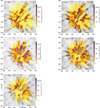 |
Fig. 5 862.1 nm DIB carrier volume density in planar surfaces parallel to the Galactic disk and at different heights: −100, −50, 0, +50 and +100 pc. The extinction density iso-contours in the same surfaces for densities 1, 2, 4, 6, 8 × 10⁻³ mag pc−1 are superimposed. |
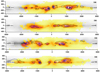 |
Fig. 6 Same as Fig. 5 for planar surfaces perpendicular to the Galactic disk and containing the Sun. oriented along various longitudes: 0−180°. 45−225°, 90−270°. and 135−315°. The extinction density iso-contours in the same surfaces for densities 1, 2.4. 6, 8 × 10⁻³ mag pc−1 are super- imposed. |
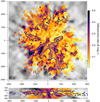 |
Fig. 7 Local values of the ratio between the DIB carrier volume density as measured by the EW local spatial gradient (in units of A pc−1) and the extinction volume density (in units of mag pc−1). The two DIB-to-dust ratio maps are for the same planes as in Figs. 3 and 4. Iso-contours of extinction density for two low values (10−1 (black) and 5 × 10⁻⁴ (violet) mag pc−1) are superimposed. |
4.2 DIB carrier and dust scale-heights or vertical distributions
The 3D maps allow us to investigate the average out-of-plane dispersion (perpendicular to the disk) in more direct ways than using integrated quantities. A first approach is to adjust an expo- nential decrease with the distance to the Plane abs(Z) at all locations in the Plane (X, Y-pairs). However, the distributions of dust and DIB carriers are strongly inhomogeneous and such a concept of scale height is somewhat inappropriate, since it requires that the density decreases on both sides of the Ζ = 0 pc horizontal plane in a quasi-exponential way, which is not the case in most locations. Even if we may adapt to the actual, wavy distribution of interstellar matter around the Plane by fitting an exponential decrease on both sides of the maximum density loca- tion (Z = Zmax, with Zmax positive or negative), in many regions there are several dense clouds at different altitudes and there is no adjustable exponential function.
To estimate the average out-of-plane dispersion of the two distributions and determine the extent to which they differ, we carried out two other calculations based on the 3D maps. First, we averaged the DIB density, the extinction density as well as their local ratio in δZ = 10 pc thick horizontal layers. We placed limits between −2000 < X < +2000 pc and −2000 < Y < +2000 pc. We found that the average ratio is minimal at Ζ ≃ +50 pc, increasing with the distance to the Plane (see Fig. 10 discussed in Sect. 4.4). More specifically, the average ratio increases by ≃20% from Ζ = −50 to +150 pc (100 pc on both sides of the minimum), by ≃40% from Ζ = −100 to +200 pc (150 pc on both sides of the minimum), and by ≃75% at abs(Z) = 300 pc. The latter increase should be taken with caution due to the low number of targets and the par- ticularly strong inhomogeneity of the distributions at such altitudes.
The second approach is was carried out as follows: for each (X, Y) pair, we extracted from the map the dust and DIB den- sity along the Ζ axis, computed separately for both quantities the altitude Zmax of the maximum density, then fit a Gaussian to the Z-dependent distribution, centred on the altitude Zmax. Although the distribution is very different from a Gaussian, such a procedure provides an order of magnitude of the dispersion on both sides of the Plane. We restricted the fits to locations (i.e., X, Y-pairs), where Zmax is between −150 pc and +150 pc. Values outside this interval are signs of very low densities and uncertain measurements. After the fitting process, we also eliminated spu- rious results induced by lack of data or by too inhomogeneous distributions such as non-converging fits, Gaussian half-widths smaller than 50 pc which trace unique clouds, or (on the con- trary) larger than 250 pc, which correspond to absence of matter along Ζ (large regions devoid of interstellar matter). We also eliminated locations for which the altitudes of the two respec- tive maxima Zmax (DIB) and Zmax (dust) were found to differ by more than 50 pc. Figure 8 shows the widths found for DIB and extinction respectively as a function of coordinates X and Y. The mean ratio between the DIB width and the extinction width was found to be 1.14. The mean Gaussian half-width at 1/e was found to be 137 pc for the DIB and 123 pc for the dust. We note that only the ratio and the order of magnitude of the width are relevant here, since (as explained above) the Gaussian function is far from closely fitting the dispersion as a function of Z.
The relative increase in dispersion along Ζ we derive is smaller than the factor of two found by Kos et al. (2014), and in closer agreement with the results of Gaia Collaboration (2023b). However, again, a strong variability of widths does exist depend- ing on quadrants, hemispheres, with a larger DIB scale height in the southern hemisphere. This may explain the results of Kos et al. (2013), as the RAVE targets are predominantly at negative latitudes.
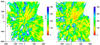 |
Fig. 8 Map of the DIB (left) and dust (right) fitted Gaussian half-widths of the out-of-plane dispersion. Units are parsec. Such DIB and dust density scale-heights perpendicular to the Galactic (XY) plane were derived by fitting a Gaussian function to the vertical (Z) distribution of DIBs and dust, respectively. The centroid of the Gaussian is fixed to Zmax, the distance above and below the Galactic plane with the highest dust density. See text for exclusion of spurious results. |
4.3 DIB to dust ratio and galactocentric distance
One interesting result from the 3D mapping is the evolution of the DIB-to-dust ratio as a function of galactocentric distance. Figure 9 shows mean values of the DIB density, the extinction density, and their ratio, averaged in cylindric shells centred on the Galactic Center (GC), each of a galactocentric distance interval of 200pc. Averages are restricted to areas that correspond to at least five targets in the inversion boxes. The size of the markers is increasing with the number of targets located in the shell. The correspondence between the size and this number is illustrated in the top graph. The ratio is increasing with the distance, namely, increasing away from the GC, at an average rate of about 15% per kpc. The trend is about the same (results not shown here) if the vertical extent of the slices is restricted to 400 pc, and 200 pc, precluding an effect of scale height difference. This is the first time a trend of this kind has been derived.
4.4 Comparisons with distributions and mass fluxes of AGB stars
It is generally thought that most of the interstellar dust is produced by dying stars during the late asymptotic giant branch (AGB) phases of their evolution. Two types of ejecta are found to coexist, namely carbon-rich and oxygen-rich dust particles. New ground-based surveys as well as Gaia measurements and subsequent analyses now make it possible for the first estimates of the two productions to be obtained. A recent catalog of the nearby AGB locations and estimates of dust production has been produced by Scicluna et al. (2022). We used the individual, estimated fluxes, and locations for each target from this catalog to compute the present C-rich and O-rich dust production in galactocentric distance bins. The results and the total production ratios are displayed in Fig. 9. Although such catalogs are still limited in target numbers, resulting in a strong variability of the ratio in the outer Galaxy, trends can be detected, namely an increase of the O-rich dust with respect to the C-rich dust in the inner Galaxy and closer to the Galactic plane (or, conversely, an increase of C-rich dust relative to O-rich dust at galactocentric distances larger than the one of the Sun). Such trends have already been noted by Quiroga-Nuñez et al. (2020); Lewis et al. (2020) and Scicluna et al. (2022). Because DIB carriers require large quantities of carbon, while dust grains need oxygen to form the silicates, this may (at least partially) explain the radial gradient and the larger dispersion of DIB molecules around the Plane with respect to the extinction we find in the maps.
Given this potential link between the galactocentric gradient of the DIB to dust ratio and the AGB distribution, we also computed the C-rich to O-rich dust flux ratio as a function of Z in 25 pc wide vertical slices, using the same catalog from Scicluna et al. (2022). The result is displayed along with the DIB to dust ratio computed in the same volumes in Fig. 10. There is a larger C/O ratio below the plane (from Z = −150 to Z = 0 pc) than above (between Z = 0 and Z = +150 pc), with a maximum at Z ≃ −50 pc. In case, this preponderance of C-rich dust at negative latitudes has an effect on the DIB density and will result in an increase of the DIB to dust ratio below the Plane; in turn, this leads to a shift of its minimum towards positive altitudes, as is observed (the minimum is found at +50 pc). Finally, from the above works, it is also inferred that the vertical distribution of AGBs is different for C-rich and O-rich types, with a larger concentration of O-type stars along the Plane and a bi-modal type distribution on both sides of the Plane for C-rich types. This may explain, at least partly, the increased density of DIB carriers, compared to dust grains, at larger distances from the Plane.
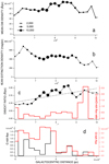 |
Fig. 9 Average values of DIB (a) and extinction (b) volume density in 100 pc thick cylindric shells for varying galactocentric distances, and their ratio (c). All cells of the 3D maps were averaged except for low density targets (back contour in Fig. 1. The size of the markers is increasing with the number of targets located in the shell. The correspondence between the size and this number is illustrated in the top graph. A linear fit to the ratio is drawn in panel c. Also shown in c is the ratio between C-rich and O-rich total fluxes from AGBs located in 265 pc thick cylindric shells, computed based on the catalog of Scicluna et al. (2022). The corresponding C- and O-rich total fluxes are displayed in panel d. |
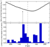 |
Fig. 10 Average values of the DIB to extinction density ratio in δZ = 10 pc horizontal slices as a function of the altitude Z (top). Ratio between C-rich and O-rich dust fluxes from AGBs, computed based on the catalog of Scicluna et al. (2022) for stars located in 25 pc wide horizontal slices (bottom). |
5 Discussion and summary
We used the recently published catalog of 862 nm DIB equivalent width measurements for individual stars, as well as corresponding Gaia positions and distances, to produce a 3D map of the DIB carrier density, using a hierarchical Bayesian inversion technique. Based on previous extinction maps, we computed the extinction towards the same series of target stars constituting the DIB catalog and performed the same inversion on the resulting extinction catalog. In doing so, we produced a 3D map of the extinction density at the same resolution at every location than for the 3D DIB map. This ensures pertinent comparisons between DIB carriers and dust volume densities.
The visual comparison between the 3D maps of DIB and dust reveals a very strong similarity, namely, regions filled with dust responsible for strong (resp. weak) optical extinction are characterized by a high (resp. low) DIB carrier density. This is not surprising, given the correlations between columns of DIB carriers and extinction. However, it is the first time it has been demonstrated in full 3D. On the other hand, there are significant differences in the relative levels of the DIB and extinction volume density, in the sense that higher than average DIB-to-dust ratios are found in areas with low dust extinction. The most conspicuous case is the wide, low-dust cavity extending in the third quadrant, which is known to be filled with warm ionized gas and where the average DIB to dust ratio is more than five times above the mean. There is a similar trend in the Local Chimney, especially below the Plane, where the gas-to-dust ratio is known to be especially low. Such a predominance of DIB carriers with respect to dust in low-extinction areas, by comparison with other regions, cannot be linked to the “skin effect” because the resolution of the map is too poor to reveal it and the areas with high DIB-to-dust ratio are much wider than the thin regions of intermediate opacity surrounding clouds and giving rise to this effect. It must be linked to other properties of the DIB carrier formation and destruction.
The full 3D maps allow us to investigate the average out-of-plane dispersion (perpendicular to the disk) in a more direct way than using integrated quantities. We averaged both the DIB and dust densities in horizontal slices of various extent and examined how these quantities and their ratios vary as a function of the distance to the Galactic plane. We found that the DIB carriers generally extend farther away from the Plane than the dust grains producing the bulk of the extinction; however, the ratios vary strongly from one location in the plane to the other and reflect the inhomogeneity of both distributions. The average ratio is minimal at Z ≃ +50 pc, increases by ≃20 % from Z = −50 to +150 pc (100 pc on both sides of the minimum), by − 40 % from Z = −100 to + 200pc (150 pc on both sides of the minimum). In a second approach, we fitted Gaussian distributions along the vertical axis Z for each (X, Y) position in the Plane. In doing so, we derived DIB and dust Gaussian half-widths (at 1/e) Hdust = 127 pc and HDIB = 133 pc. This again shows that the average dispersion around the Plane is larger for the molecules than for the dust grains, with an average relative difference of 11% for the widths. This is less than the factor of two found by Kos et al. (2014), and in closer agreement with Gaia Collaboration (2023b). However, a strong variability of widths does exist depending on areas, with a larger scale height in the southern hemisphere. This may explain the results of Kos et al. (2013), as the RAVE targets are predominantly at negative latitudes.
Finally, we averaged densities and ratios in cylindric shells whose axes are vertical and contain the GC, for various galac-tocentric distances and found that the DIB to dust ratio is increasing radially (see Fig. 9). The average gradient is around 15% per kpc in the Sun vicinity. The potential explanation for this new result cannot be linked to the radial gradient of metallicity, which (according to Magellanic clouds studies) is expected to produce an effect opposite to what is observed.
Although our conclusions are limited by the resolution of the maps, the observed trends deserve attention. The first result is the apparently generalized increase of the 860.2 nm DIB-to-extinction ratio in low-dust areas (see Fig. 7). If the macro-molecule at the origin of the DIB is one of the numerous products of the very rich chemistry occurring at the surface of icy grains in dense cloud cores, the results suggest that once they have been released from the grains in the gas (due to shock or radiation), these molecules survive during a period of time long enough to be detected away from the clouds in low density regions. This implies a strong resilience of the 860.2 nm DIB carriers at locations where dust grains are partly destroyed. If 860.2 nm DIB carriers would instead have been built gradually in stellar ejecta and in the diffuse interstellar medium, they would have to be preferentially associated with grains smaller than those responsible for the extinction in the visible. The same types of conclusions are drawn from the DIB out-of-plane dispersion, found to be in average higher than the dust dispersion. The DIB carriers produced in dense areas close to the Galactic plane may be released at higher altitude and maintained far from the dense clouds in lower density gas where grains are destroyed or settle down to the Plane by gravity. In both cases, dust-poor regions or regions above or below the disk, the observed trends imply that the DIB carrier density follows the gas density and not solely the dust concentration.
We investigated the potential role of the spatial distribution of AGB stars. Their distribution in the Milky Way is increasingly well measured thanks to Gaia. New observations distinguish the oxygen-rich (O-type) and carbon-rich (C-type) AGB stars from each other and recent analyses from space and ground have shown that in the vicinity of the Sun, O-rich AGB stars are predominant in the inner Galaxy and close to the Plane. C-rich dust is expected to favour the formation of the DIB carriers, while O-rich ejecta are needed to form silicate grains. We used the catalog of Scicluna et al. (2022) and inferred that the production of C-rich dust is increasing radially by comparison with O-rich dust, in agreement with the direction of the DIB to dust gradient we observe here. Interestingly, the same catalog shows an increased production of C-rich dust below the Plane (over the first 100 pc), which could be linked to the observed location of the minimum DIB to dust ratio above the Plane, shifted to Z = + 50 pc. Finally, the bi-modal vertical distribution of C-rich AGB stars with maxima on both sides of the Plane, at variance with the maximal concentration of O-rich stars close to Z = 0 pc, may potentially (and at least partly) explain the larger dispersion around the Plane of DIBs with respect to grains.
While our results are still limited by the map resolution and ought to be confirmed in future works, the potential link we find with C-rich AGB stars show that full 3D mapping of DIB absorption data opens the way to new diagnostics about the processes involving their carriers. Ongoing and future massive spectroscopic surveys will enable the application of the 3D mapping technique to stronger and narrower DIBs to produce more resolved maps and test differences among the various DIBs; meanwhile, parallel improvements with respect to stellar catalogs are expected to help confirm (or otherwise) purported links with various types of stars and environments.
Acknowledgements
We thank our referee Tomaz Zwitter for useful comments and criticisms. This project has received funding from the European Union’s Horizon 2020 research and innovation programme under grant agreement No 101004214 (EXPLORE project – https://explore-platform.eu). This article/publication is based upon work from COST Action CA21126 – Carbon molecular nanostructures in space (NanoSpace), supported by COST (European Cooperation in Science and Technology). This work has made use of data from the European Space Agency (ESA) mission Gaia (https://www.cosmos.esa.int/gaia), processed by the Gaia Data Processing and Analysis Consortium (DPAC, https://www.cosmos.esa.int/web/gaia/dpac/consortium). Funding for the DPAC has been provided by national institutions, in particular the institutions participating in the Gaia Multilateral Agreement. This research has made use of the VizieR catalog access tool, CDS, Strasbourg, France (DOI: 10.26093/cds/vizier). The original description of the VizieR service is published in Ochsenbein et al. (2000).
Appendix A Additional figure
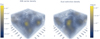 |
Fig. A.1 Volume rendering of the diffuse interstellar band carrier (left) and dust (right) for a sub-region of the full 3D data. The centre of the 3d volume plot is X = −1000 pc, Y = −1000 pc, Z = −102.5 pc, with size of 400 pc in X and Y, and 200 pc in Z. Density surfaces color-coded. The full cube can be explored by downloading from Zenodo or viewed using the interactive tool G-Tomo on https://explore-platform.eu. |
References
- Baron, D., Poznanski, D., Watson, D., Yao, Y., & Prochaska, J. X. 2015, MNRAS, 447, 545 [NASA ADS] [CrossRef] [Google Scholar]
- Cami, J., & Cox, N. L. J., eds. 2014, IAU Symposium, 297, The Diffuse Interstellar Bands [Google Scholar]
- Campbell, E. K., Holz, M., Gerlich, D., & Maier, J. P. 2015, Nature, 523, 322 [NASA ADS] [CrossRef] [Google Scholar]
- Chen, B. Q., Huang, Y., Yuan, H. B., et al. 2019, MNRAS, 483, 4277 [Google Scholar]
- Cordiner, M. A., Cox, N. L. J., Evans, C. J., et al. 2011, ApJ, 726, 39 [NASA ADS] [CrossRef] [Google Scholar]
- Cordiner, M. A., Linnartz, H., Cox, N. L. J., et al. 2019, ApJ, 875, L28 [NASA ADS] [CrossRef] [Google Scholar]
- Elyajouri, M., Cox, N. L. J., & Lallement, R. 2017, A&A, 605, L10 [NASA ADS] [CrossRef] [EDP Sciences] [Google Scholar]
- Ensor, T., Cami, J., Bhatt, N. H., & Soddu, A. 2017, ApJ, 836, 162 [Google Scholar]
- Fan, H., Welty, D. E., York, D. G., et al. 2017, ApJ, 850, 194 [NASA ADS] [CrossRef] [Google Scholar]
- Fan, H., Hobbs, L. M., Dahlstrom, J. A., et al. 2019, ApJ, 878, 151 [NASA ADS] [CrossRef] [Google Scholar]
- Farhang, A., van Loon, J. T., Khosroshahi, H. G., Javadi, A., & Bailey, M. 2019, Nat. Astron., 3, 922 [NASA ADS] [CrossRef] [Google Scholar]
- Foing, B. H., & Ehrenfreund, P. 1994, Nature, 369, 296 [NASA ADS] [CrossRef] [Google Scholar]
- Friedman, S. D., York, D. G., McCall, B. J., et al. 2011, ApJ, 727, 33 [NASA ADS] [CrossRef] [Google Scholar]
- Gaia Collaboration (Prusti, T., et al.) 2016, A&A, 595, A1 [NASA ADS] [CrossRef] [EDP Sciences] [Google Scholar]
- Gaia Collaboration (Schultheis, M., et al.) 2023a, A&A, 680, A38 [NASA ADS] [CrossRef] [EDP Sciences] [Google Scholar]
- Gaia Collaboration (Schultheis, M., et al.) 2023b, A&A, 674, A40 [CrossRef] [EDP Sciences] [Google Scholar]
- Gaia Collaboration (Vallenari, A., et al.) 2023c, A&A, 674, A1 [NASA ADS] [CrossRef] [EDP Sciences] [Google Scholar]
- Green, G. M., Schlafly, E., Zucker, C., Speagle, J. S., & Finkbeiner, D. 2019, ApJ, 887, 93 [NASA ADS] [CrossRef] [Google Scholar]
- Heckman, T. M., & Lehnert, M. D. 2000, ApJ, 537, 690 [NASA ADS] [CrossRef] [Google Scholar]
- Kos, J., Zwitter, T., Grebel, E. K., et al. 2013, ApJ, 778, 86 [NASA ADS] [CrossRef] [Google Scholar]
- Kos, J., Zwitter, T., Wyse, R., et al. 2014, Science, 345, 791 [NASA ADS] [CrossRef] [Google Scholar]
- Lallement, R. 2015, Journal of Physics Conference Series, 577, 012016 [NASA ADS] [CrossRef] [Google Scholar]
- Lallement, R., Vergely, J. L., Babusiaux, C., & Cox, N. L. J. 2022, A&A, 661, A147 [NASA ADS] [CrossRef] [EDP Sciences] [Google Scholar]
- Lan, T.-W., Ménard, B., & Zhu, G. 2015, MNRAS, 452, 3629 [Google Scholar]
- Leger, A., & D’Hendecourt, L. 1985, A&A, 146, 81 [Google Scholar]
- Leike, R. H., Glatzle, M., & Enßlin, T. A. 2020, A&A, 639, A138 [NASA ADS] [CrossRef] [EDP Sciences] [Google Scholar]
- Lewis, M. O., Pihlström, Y. M., Sjouwerman, L. O., et al. 2020, ApJ, 892, 52 [NASA ADS] [CrossRef] [Google Scholar]
- Monreal-Ibero, A., Weilbacher, P. M., Wendt, M., et al. 2015, A&A, 576, A3 [Google Scholar]
- Ochsenbein, F., Bauer, P., & Marcout, J. 2000, A&AS, 143, 23 [NASA ADS] [CrossRef] [EDP Sciences] [Google Scholar]
- Phillips, M. M., Simon, J. D., Morrell, N., et al. 2013, ApJ, 779, 38 [NASA ADS] [CrossRef] [Google Scholar]
- Puspitarini, L., Lallement, R., Babusiaux, C., et al. 2015, A&A, 573, A35 [NASA ADS] [CrossRef] [EDP Sciences] [Google Scholar]
- Quiroga-Nunez, L. H., van Langevelde, H. J., Sjouwerman, L. O., et al. 2020, ApJ, 904, 82 [CrossRef] [Google Scholar]
- Rezaei Kh., S., Bailer-Jones, C. A. L., Soler, J. D., & Zari, E. 2020, A&A, 643, A151 [EDP Sciences] [Google Scholar]
- Sarre, P. J., Miles, J. R., Kerr, T. H., et al. 1995, MNRAS, 277, L41 [NASA ADS] [Google Scholar]
- Saydjari, A. K., Uzsoy, A. S. M., Zucker, C., Peek, J. E. G., & Finkbeiner, D. P. 2023, ApJ, 954, 141 [NASA ADS] [CrossRef] [Google Scholar]
- Scicluna, P., Kemper, F., McDonald, I., et al. 2022, MNRAS, 512, 1091 [NASA ADS] [CrossRef] [Google Scholar]
- Snow, T. P. J., & Cohen, J. G. 1974, ApJ, 194, 313 [NASA ADS] [CrossRef] [Google Scholar]
- Vergely, J. L., Freire Ferrero, R., Siebert, A., & Valette, B. 2001, A&A, 366, 1016 [NASA ADS] [CrossRef] [EDP Sciences] [Google Scholar]
- Vergely, J. L., Lallement, R., & Cox, N. L. J. 2022, A&A, 664, A174 [NASA ADS] [CrossRef] [EDP Sciences] [Google Scholar]
- Vos, D. A. I., Cox, N. L. J., Kaper, L., Spaans, M., & Ehrenfreund, P. 2011, A&A, 533, A129 [NASA ADS] [CrossRef] [EDP Sciences] [Google Scholar]
- Zasowski, G., Ménard, B., Bizyaev, D., et al. 2015, ApJ, 798, 35 [Google Scholar]
All Figures
|
Fig. 1 Coverage of sources in the input catalog along the Galactic plane. The number of sources per 1003 pc3 cell is color-coded. All sources with abs(z) <50 pc are included. The limit of five targets per cell used in the statistical study is marked by a thick black line. |
| In the text | |
|
Fig. 2 Aitoff projection of the maximum reliable distance map for the DIB 3d reconstruction. Iso-Galactic longitudes and latitudes are drawn spaced by 30°. The Galactic Center (l = 0) is at the center and longitudes are increasing to the left. The reconstruction in the Galactic plane (|b| < 15°) has the highest fidelity. |
| In the text | |
|
Fig. 3 862.1 nm DIB carrier volume density (left) and extinction volume density (right) in the plane parallel to the Galactic plane and containing the Sun. Coordinates are in parsec from the Sun location. The Galactic Center is to the right and the longitude increases anti-clockwise. Dashed lines are iso-galactocentric distances spaced by 1000 pc. The central line corresponds to the Sun location and X = 0. Black and white coded regions correspond to those with low target densities and more uncertain measurements. |
| In the text | |
|
Fig. 4 Same as Fig. 3 for a vertical plane containing the Sun and the Galactic centre direction (to the right). The North Galactic Pole (NGP) is at the top. Color-coding is the same as in Fig. 3. |
| In the text | |
|
Fig. 5 862.1 nm DIB carrier volume density in planar surfaces parallel to the Galactic disk and at different heights: −100, −50, 0, +50 and +100 pc. The extinction density iso-contours in the same surfaces for densities 1, 2, 4, 6, 8 × 10⁻³ mag pc−1 are superimposed. |
| In the text | |
|
Fig. 6 Same as Fig. 5 for planar surfaces perpendicular to the Galactic disk and containing the Sun. oriented along various longitudes: 0−180°. 45−225°, 90−270°. and 135−315°. The extinction density iso-contours in the same surfaces for densities 1, 2.4. 6, 8 × 10⁻³ mag pc−1 are super- imposed. |
| In the text | |
|
Fig. 7 Local values of the ratio between the DIB carrier volume density as measured by the EW local spatial gradient (in units of A pc−1) and the extinction volume density (in units of mag pc−1). The two DIB-to-dust ratio maps are for the same planes as in Figs. 3 and 4. Iso-contours of extinction density for two low values (10−1 (black) and 5 × 10⁻⁴ (violet) mag pc−1) are superimposed. |
| In the text | |
|
Fig. 8 Map of the DIB (left) and dust (right) fitted Gaussian half-widths of the out-of-plane dispersion. Units are parsec. Such DIB and dust density scale-heights perpendicular to the Galactic (XY) plane were derived by fitting a Gaussian function to the vertical (Z) distribution of DIBs and dust, respectively. The centroid of the Gaussian is fixed to Zmax, the distance above and below the Galactic plane with the highest dust density. See text for exclusion of spurious results. |
| In the text | |
|
Fig. 9 Average values of DIB (a) and extinction (b) volume density in 100 pc thick cylindric shells for varying galactocentric distances, and their ratio (c). All cells of the 3D maps were averaged except for low density targets (back contour in Fig. 1. The size of the markers is increasing with the number of targets located in the shell. The correspondence between the size and this number is illustrated in the top graph. A linear fit to the ratio is drawn in panel c. Also shown in c is the ratio between C-rich and O-rich total fluxes from AGBs located in 265 pc thick cylindric shells, computed based on the catalog of Scicluna et al. (2022). The corresponding C- and O-rich total fluxes are displayed in panel d. |
| In the text | |
|
Fig. 10 Average values of the DIB to extinction density ratio in δZ = 10 pc horizontal slices as a function of the altitude Z (top). Ratio between C-rich and O-rich dust fluxes from AGBs, computed based on the catalog of Scicluna et al. (2022) for stars located in 25 pc wide horizontal slices (bottom). |
| In the text | |
|
Fig. A.1 Volume rendering of the diffuse interstellar band carrier (left) and dust (right) for a sub-region of the full 3D data. The centre of the 3d volume plot is X = −1000 pc, Y = −1000 pc, Z = −102.5 pc, with size of 400 pc in X and Y, and 200 pc in Z. Density surfaces color-coded. The full cube can be explored by downloading from Zenodo or viewed using the interactive tool G-Tomo on https://explore-platform.eu. |
| In the text | |
Current usage metrics show cumulative count of Article Views (full-text article views including HTML views, PDF and ePub downloads, according to the available data) and Abstracts Views on Vision4Press platform.
Data correspond to usage on the plateform after 2015. The current usage metrics is available 48-96 hours after online publication and is updated daily on week days.
Initial download of the metrics may take a while.