| Issue |
A&A
Volume 689, September 2024
|
|
|---|---|---|
| Article Number | A210 | |
| Number of page(s) | 13 | |
| Section | Extragalactic astronomy | |
| DOI | https://doi.org/10.1051/0004-6361/202449839 | |
| Published online | 13 September 2024 | |
The fate of the interstellar medium in early-type galaxies
IV. The impact of stellar feedback, mergers, and black holes on the cold interstellar medium in simulated galaxies
1
Astronomical Observatory Institute, Faculty of Physics, Adam Mickiewicz University, ul. Słoneczna 36, 60-286
Poznań, Poland
2
Institute for Astronomy, University of Edinburgh, Royal Observatory, Blackford Hill, Edinburgh, EH9 3HJ
UK
3
SISSA, Via Bonomea 265, 34136
Trieste, Italy
4
INAF, Osservatorio Astronomico di Trieste, Via Tiepolo 11, 34131
Trieste, Italy
5
DARK, Niels Bohr Institute, University of Copenhagen, Jagtvej 155A, 2200
Copenhagen N, Denmark
Received:
2
March
2024
Accepted:
19
June
2024
Abstract
Context. Removing the cold interstellar medium (ISM) from a galaxy is essential to quenching star formation, however, the exact mechanism behind this process remains unclear.
Aims. The objective of this work is to find the mechanism responsible for dust and gas removal in simulated early-type galaxies.
Methods. We studied a statistically significant sample of massive (M* > 1010 M⊙), simulated early-type galaxies in a redshift range of 0.02−0.32 in the context of its ISM properties. In particular, we investigated the cold dust and gas removal timescales, the cold gas inflows, and their relation with black hole mass. We also investigated the evolution of galaxies in the dust mass and star formation rate (SFR) plane and the influence of merger events. Finally, we broke down the dust destruction mechanisms to find which (if any) of the implemented processes dominate as a function of a galaxy’s stellar age.
Results. We find a good agreement with previous observational works dealing with the timescales of dust and HI removal from early-type galaxies. When considering the dust-to-stellar-mass ratio as a function of time in simulations, we recovered a similar decline as in the observational sample as a function of stellar age, validating its use for timing the ISM decline. Moreover, we recovered the observed relation between dust mass and the SFR for actively star-forming galaxies, as well as that of passive early-type galaxies. We also show that starburst galaxies form their own sequence on the dust mass and SFR plot in the form of log(Mdust, SB) = 0.913 × log(SFR)+6.533, with a 2σ scatter of 0.32. Finally, we find that type II supernova reverse shocks dominate the dust destruction at the early stages of early-type galaxy evolution; however, we also see that at later times, stellar feedback becomes more important. We show that merger events lead to morphological transformations by increasing the bulge-to-total stellar mass ratio, followed by an increase in black hole masses. The black hole feedback resulting from radio mode accretion prevents the hot halo gas from cooling, indirectly leading to a decrease in the SFR.
Key words: galaxies: elliptical and lenticular / cD / galaxies: evolution / galaxies: ISM / galaxies: starburst / galaxies: star formation
Corresponding author; This email address is being protected from spambots. You need JavaScript enabled to view it. .
© The Authors 2024
 Open Access article, published by EDP Sciences, under the terms of the Creative Commons Attribution License (https://creativecommons.org/licenses/by/4.0), which permits unrestricted use, distribution, and reproduction in any medium, provided the original work is properly cited.
This article is published in open access under the Subscribe to Open model. This email address is being protected from spambots. You need JavaScript enabled to view it. to support open access publication.
1. Introduction
Galaxy quenching is the process by which star formation activity decreases significantly or stops altogether. This cessation of star formation has a profound impact on the fundamental processes that govern the galaxy evolution. This is why significant efforts are dedicated to finding the primary mechanism responsible for quenching, while also considering the possibility that there could be multiple mechanisms at work.
To stop star formation in a galaxy, it is necessary to either prevent gas inflows, remove or destroy the cold interstellar medium (ISM), or make the cold gas unable to form stars. To date, several processes have been proposed. These mechanisms operate on different time and physical scales (Bell et al. 2012; Cheung et al. 2012; Hjorth et al. 2014). A schematic illustration was presented by Man & Belli (2018), where the authors identified five broad classes of quenching mechanisms: (1) gas does not accrete onto the galaxy; (2) gas does not cool; (3) cold gas does not form stars; (4) cold gas is rapidly consumed; and (5) gas is removed.
Cold interstellar gas can be consumed by star formation (astration; Peng et al. 2015), or it can be ionised either by supernovae (SNe; Dekel & Silk 1986; Muratov et al. 2015) or hot low-mass evolved stars (Herpich et al. 2018). Additionally, active galactic nuclei (AGNs) can be responsible for heating and removing considerable amounts of gas leading to the quenching of star formation (Di Matteo et al. 2005; Piotrowska et al. 2022). It has also been shown that morphological transformation can stop star formation by merger events and by building up the bulge (Schawinski et al. 2014). This bulge stabilizes gas and prevents it from collapsing, leaving the galaxy as a bulge-dominated, elliptical, compact early-type galaxies (ETGs; see mass-size relation, e.g. Mowla et al. 2019; Nadolny et al. 2021). This process is known as morphological quenching (Martig et al. 2009; Gensior et al. 2020).
With respect to dust, several processes governing its production and destruction have been proposed. Such production processes include: circumstellar shells around evolved stars such as asymptotic giant branch stars or red giants, SN remnants, and other non-stellar processes like grain growth in the ISM (Knapp et al. 1992; Jones 2004; Matsuura et al. 2011; Morgan & Edmunds 2003; Gall et al. 2011; Nanni et al. 2013; Michałowski et al. 2010; Michałowski 2015; Leśniewska & Michałowski 2019). The destruction processes include astration, SN reverse shock waves, ionising emission from planetary nebulae (PNs), galactic outflows, or AGNs (Bianchi & Ferrara 2005; Clemens et al. 2010; Gall & Hjorth 2018; Michałowski et al. 2019) acting through sputtering, shattering, and evaporation. See also reviews by Jones (2004) and Gall et al. (2011) and references therein.
In addition to the mentioned mechanisms acting on the ISM within a galaxy, an external origin to explain the evolution of the ISM has also been proposed for ETGs. This newly accreted gas (e.g. from mergers) may trigger star formation with short depletion times (leading to starbursts; Nadolny et al. 2023). As a consequence, it may then lead to the production and destruction of dust (van Gorkom et al. 1989; Naab et al. 2006; López-Sanjuan et al. 2012). Thus, the determination of the ISM removal timescale, τ, is essential to improving our understanding of the specific process that plays a major role in the quenching of star formation.
Due to the destruction, recycling, and replenishing of the gas and dust content in actively star-forming galaxies (Donevski et al. 2020), it is challenging to estimate τ for this galaxy population. As shown via high-resolution hydrodynamical simulations (Segovia Otero et al. 2022), the emergence of a galactic disc and the dominance of rotational velocity over dispersion velocity enables bursts of star formation. Therefore, following Michałowski et al. (2019), the most appropriate sample to study the ISM removal timescale is a sample of galaxies with detectable dust or gas, along with a low star formation rate (SFR). These are characteristics of ETGs that are mostly found below the main sequence (MS) of star-forming galaxies (SFGs). Furthermore, Magdis et al. (2021) showed passive evolution of dust-to-stellar mass ratio for quiescent galaxies between z ∼ 2 and 1, with a steep decrease with decreasing redshift. This decrease is much steeper as compared to SFG at low-z.
In the last few decades, a great effort has been made to tackle the quenching mechanism in the framework of cosmological simulations. Within the whole spectrum of different types of simulations, two main branches have emerged. One of these are simulations based on semi-analytic models (SAMs; De Lucia et al. 2004; De Lucia & Blaizot 2007; Springel et al. 2005; Henriques et al. 2015). The second type are hydrodynamical simulations (Vogelsberger et al. 2014; Hopkins et al. 2014; Schaye et al. 2015; Pillepich et al. 2018; Whitaker et al. 2021; Segovia Otero et al. 2022; Lorenzon et al. 2024). Each type of simulation focuses on different spatial and temporal scales, with different mass resolutions.
In this work, we investigate the atomic hydrogen HI gas and dust removal timescales using the L-GALAXIES2020 SAM (Henriques et al. 2020). In particular, we adopted the Parente et al. (2023) version of the model, which includes a detailed treatment of dust evolution within galaxies. The SAM parameters have been tuned to reproduce a broad range of galaxy properties (Henriques et al. 2020; Parente et al. 2023), but not the main quantities analyzed in this work, namely, the dust (and gas) removal timescales. Therefore, we employed our SAM to provide a robust physical interpretation of observations, particularly concerning the quenching mechanism and dust-related processes. Our goal of this study is to investigate the ISM behavior in simulated ETGs. In particular, we study ISM removal timescales and the influence of stellar mass, BH mass, and redshift on the ISM. Furthermore, we study the evolution of individual galaxies in the dust mass versus SFR plane. Finally, we investigate the mechanisms of the destruction and removal of dust in the selected galaxy samples.
This article is organised as follows. In Sect. 2, we present the observational and simulated data, together with a short description of the essential characteristics of the L-GALAXIES2020 models. In Sect. 3, we present the results of the dust and HI removal timescales for the selected sample (Sect. 3.1) for the sample divided in bins of different parameters (Sect. 3.2) and results for individual galaxies (Sect. 3.3). In Sect. 3.4, we describe our results in terms of the global relation between dust mass and SFR, also considering the evolution of individual galaxies. In Sect. 3.5, we examine several dust destruction and removal mechanisms. In Sect. 4, we present our discussion and conclusions. Throughout this paper, we use a cosmological model with h = 0.673, ΩΛ = 0.685, and Ωm = 0.315 (Planck Collaboration XVI 2014). The initial mass function (IMF) from Chabrier (2003) was assumed in the applied SAM.
2. Data
2.1. Observational data
In this work, we made use of samples defined in Leśniewska et al. (2023) and Michałowski et al. (2024). In particular, Leśniewska et al. (2023) studied the dust-to-stellar mass ratio as a function of stellar age of observed ETGs (hereafter the GAMA sample), whereas Michałowski et al. (2024) studied the H I-to-stellar mass ratio as a function of stellar age. We refer to these works for details on the data used. In short, both samples were selected based on similar criteria: (i) early-type morpologies were selected using a Sérsic index (Sérsic 1963) with values higher than four (n > 4) in Leśniewska et al. (2023) or visual early-type morphology in Michałowski et al. (2024; ii) a redshift range between 0.02 and 0.32 was selected to ensure that at higher redshifts the Sérsic index selection does not include bulge-dominated or compact late-type galaxies (LTGs); and (iii) for the dust detection, we followed both Leśniewska et al. (2023) and Michałowski et al. (2024), where a signal-to-noise (S/N) threshold at 250 μm of 3 was used. Due to the size of the GAMA sample, it was used as a reference for our L-GALAXIES2020 sample selection.
2.2. Simulations
In this work, we make use of the predictions of the L-GALAXIES2020 SAM, which is the latest version of the Munich semi-analytic model for galaxy evolution (Henriques et al. 2015, 2020). In particular, we adopted the version introduced by Parente et al. (2023), which accounts for a detailed model for dust production and evolution, as well as for an updated treatment of disc instabilities. In this section, we summarise the main features of this SAM, while we refer to the supplementary material of Henriques et al. (2020) for a detailed description of all these processes.
The L-GALAXIES2020 model starts from the dark matter (DM) haloes merger trees of the MILLENNIUM simulation (Springel et al. 2005) and populates them with baryons according to a number of physical processes, which are important for galaxy evolution. Among them are gas infall into DM haloes, gas cooling, disc and bulge formation, star formation, merger-driven starbursts, chemical enrichment, energetic feedback from stars and supermassive black holes (SMBHs), and environmental processes such as ram pressure and tidal stripping.
The ISM is represented by a disc which results from the (metallicity and temperature dependent) cooling of the hot halo gas. Such a disc is spatially resolved: gas properties are tracked for each simulated object in 12 concentric rings. For each of them, the SAM determines the molecular fraction of the ISM according to the Krumholz et al. (2009) model. Subsequently, this H2 mass fuels the star formation (Gao & Solomon 2004; Wong & Blitz 2002). The star formation law implemented in the L-GALAXIES2020 is based on the H2 surface density (Bigiel et al. 2011; Leroy et al. 2013). An inverse dependency of star formation on the dynamical time (Sect. 2.2.4 in Henriques et al. 2020) has also been implemented. This ensures that star formation is more efficient for galaxies with shorter dynamical times, in particular at earlier epochs (Scoville et al. 2017). The stars produce energetic and chemical feedback, which was modelled according to Yates et al. (2013). This model traces the abundances of eleven chemical elements (H, He, C, N, O, Ne, Mg, Si, S, Ca, and Fe) produced in supernovae (SNe type Ia and II) and in asymptotic giant branch (AGB) stars released by their winds. Both the feedback and chemical enrichment are modelled separately for each ring of the disc. Tracing the evolution of baryons in each ring is essential for the evaluation of the chemical evolution, H2 fraction, and SFRs. For this work, however, we use integrated properties (e.g. total stellar mass, total SFR, and total dust mass) of the selected sample – and not the values evaluated for each ring.
In addition, star formation is sensitive to merger events that may trigger a burst of star formation. As for the descendant galaxy, the SAM models different outcomes for minor and major mergers. In a major merger, the discs of the progenitors are destroyed, and all the stars form the bulge of the resulting (descendent) galaxy. Any star that forms during this event is added to the bulge, increasing its mass. During a minor merger, the disc of a larger progenitor survives and accretes the cold gas from the smaller galaxy. All the stars from the smaller galaxy are included in the bulge, while newly formed stars are added to the disc of the descendant galaxy. Thus both minor and major mergers shape the morphology of a galaxy, in particular by increasing the bulge mass.
Disc instabilities can also result in the bulge growth, although they mostly affect the morphology of intermediate-mass galaxies. The modelling of this process has been revised in the SAM version we adopt (Parente et al. 2023), leading to a better agreement with the observed abundance of local galaxies with different morphologies.
Merger events and disc instabilities1 also drive the growth of the central SMBHs. In the L-GALAXIES2020 the growth of a BH is through radio or quasar mode. While the quasar mode is mostly responsible for the black hole growth, in the adopted SAM it produces no feedback. On the other hand, the radio mode accretion of the hot gas provides feedback that increases with increasing black hole mass and hot gas mass (Sect. 1.14.2 of the supplementary material of Henriques et al. 2020). The radio mode feedback is crucial since it leads to the quenching of star formation by preventing hot gas from cooling (Henriques et al. 2017).
Finally, the SAM self-consistently models the formation and evolution of dust grains within galaxies. The dust model was introduced in Parente et al. (2023, with details given in their Sect. 2.1). It was inspired by state-of-the-art models already successfully adopted in hydrodynamical simulations (Granato et al. 2021; Parente et al. 2022). The model is based on the two-size approximation (Hirashita 2015) and it follows the evolution of two sizes and two chemical compositions of grains (i.e. silicate and carbonaceous, MgFeSiO4 and C, with radii of 0.05 and 0.005 μm) In short, large grains are assumed to be produced by AGB stars and type II SNe and are then ejected into the cold and hot gas of galaxies. Different processes that affect the evolution of grains are modelled in the SAM. These include grain growth by accretion of gas-phase metals, destruction by (type Ia and II) SN explosions with a part of the energy released used for heating of the gas which is then transferred from the cold phase to the hot atmosphere together with corresponding dust (see Parente et al. 2023 and supplementary material in Henriques et al. 2020 for details). Furthermore sputtering in the hot gas, as well as shattering (coagulation) of large (small) grains is also implemented. The modelling of these processes is done on the fly and through physically motivated recipes which depend on the physical properties of the gas phase of simulated galaxies. This model has been shown to reproduce several scaling relations involving dust at z < 2.5 and (notably in the context of this work) the dust abundance in LTGs and ETGs at z = 0.
2.3. Sample selection
The selection process of the simulated sample of ETGs has been designed to closely follow the selection of galaxies studied in the observational works to which we are comparing our results. Our selection was undertaken based on the following criteria: (i) redshift range between 0.02 and 0.32; (ii) bulge-to-total stellar mass ratio above 0.7; and (iii) dust mass above the dust mass limit estimated using the GAMA sample to mimic their 250 μm S/N limit. This dust mass limit is estimated using a polynomial fit to the GAMA sample dust mass as a function of redshift (Fig. 1, dashed line on the right panel) and shifted 2σ downwards; it is given as:

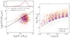 |
Fig. 1. SFR as a function of stellar mass (left). The solid line shows the MS from the L-GALAXIES2020 simulations estimated using LTGs (see main text for details) and is a power-law fit described as log(SFR) = a × log(M*)+b with coefficients given in the legend. The dotted line shows the MS estimated using a prescription from Speagle et al. (2014), both at z = 0.18. Orange and gray points show the GAMA, and L-GALAXIES2020 ETG samples. Normalised stellar mass distribution for the mentioned samples (top). Dust mass as a function of redshift (right). The dashed line shows the dust mass limit estimated for the GAMA sample. More details are given in Sect. 2.3. |
where z is redshift. Finally, we have (iv) a random selection of galaxies in eight redshift bins (with a width of 0.15) to follow the redshift distribution of the observed GAMA sample.
After this selection process, our ETG L-GALAXIES2020 sample contains 2050 galaxies. This is the exact number of galaxies as presented in Leśniewska et al. (2023) with very similar physical properties that allow precise comparison. We show the selected galaxies in Fig. 1. We note that the stellar masses and dust masses of the selected ETGs are slightly lower (on average) by 0.12 dex and 0.2 dex, respectively, as compared to Leśniewska et al. (2023). In particular, for the same stellar mass, the simulated galaxies have, on average, 0.3 dex lower dust mass.
In the left panel in Fig. 1, we compare the MS estimated using a prescription from Speagle et al. (2014) at z = 0.18, namely, the same as used in Leśniewska et al. (2023), and the MS estimated from simulated LTGs. These simulated LTGs were selected by imposing a bulge-to-total mass ratio below 0.3 and z = 0.18. Using a standard 0.2 dex scatter we find that 68% of our ETGs are found below the MS, consistently with Leśniewska et al. (2023). We describe this particular selection in Sect. 3.4 in the context of the da Cunha et al. (2010) relation.
3. Results
3.1. ISM removal timescales
The dust and gas removal timescales are determined using an exponential function in the form (Michałowski et al. 2019) of:
 (1)
(1)
where Mass stands for dust or HI gas masses, A is a normalisation constant, and τ is the ISM removal timescale. We fit this exponential function to the dust-to-stellar and H I-to-stellar mass ratios and obtained the results shown in Fig. 2, together with the observational results. We found dust (τd) and HI (τHI) removal timescales of 2.28 ± 0.1 Gyr and 1.92 ± 0.09 Gyr, respectively. Errors given in this work have been estimated as a standard deviation of resulting τ from 1000 Monte Carlo runs, where we perturbed the mass ratio for all galaxies independently by a randomly selected value from a Gaussian distribution centered at μ = 0 and with a width defined as a standard deviation of a distance from the best-fit line. The resulting dust and HI removal timescales are in excellent agreement with the results from Leśniewska et al. (2023), where they found τd = 2.26 ± 0.22 Gyr, and τHI = 1.97 ± 0.10 from Michałowski et al. (2024). Our analysis of the selected simulated galaxies using the L-GALAXIES2020 SAM is the first (to our knowledge) effort to estimate the dust and HI dust removal timescales in the same way as was done for the observed samples. Similar result was found in hydrodynamical simulations in very recent work by Lorenzon et al. (2024).
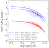 |
Fig. 2. HI-to-stellar and dust-to-stellar mass ratios as a function of light-weighted stellar age. Exponential fits to L-GALAXIES2020 ETG samples (dashed lines), together with observationally derived fits from Michałowski et al. (2024), Leśniewska et al. (2023) (continuous and dotted lines) are shown. |
3.2. ISM removal timescales and galaxy properties
In this section, we test whether other galaxy properties affect the ISM removal. In particular, we investigate the mass ratio dependence on stellar mass, black hole (BH) mass, and redshift (see Fig. 3). The dust removal timescales vary between 2.03 and 3.05 Gyr; however, most of these are consistent within the errors and the normalisation of the dust-to-stellar mass ratio remains roughly constant in all cases (as compared to the fit to our full ETG sample, shown as a red dashed line).
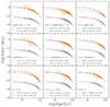 |
Fig. 3. HI-to-stellar and dust-to-stellar mass ratio as a function of light-weighted age. Orange and grey lines show fits to HI- and dust-to-stellar mass ratios for sub-samples divided into stellar mass (top row), the black hole-to-stellar mass ratio (middle), and redshift (bottom row) bins. Blue and red dashed lines show fits to the overall ETG sample from Fig. 2 and are given for reference. |
In the case of HI, the variation in the removal timescale and the normalisation is visible, in particular when using stellar and BH mass bins. The τHI difference, however, is not statistically significant. For the stellar (BH) mass bins, the H I-to-stellar mass ratio normalisation constants, A, are 0.20 ± 0.12 (0.18 ± 0.13), −0.42 ± 0.05 (−0.22 ± 0.04), and −0.58 ± 0.12 (−0.31 ± 0.1) from the low to high stellar (BH) mass. The normalisation for the entire sample for H I-to-stellar mass ratio fit is A = 0.04 ± 0.06, while the same normalisation constant from Michałowski et al. (2024) is A = 0.37 ± 0.05. These differences in the normalisation constant A in stellar mass bins reflect the correlation of the gas-to-dust mass ratio with metallicity, as shown in Rémy-Ruyer et al. (2014); namely, it is evident that more massive (and more metal-rich as a result of the well-known mass-metallicity relation; e.g. Lara-López et al. 2010; Nadolny et al. 2020) galaxies have lower gas-to-dust ratios. Moreover, this relation was successfully reproduced (using the SAM employed in this work) in Parente et al. (2023). To test that, we analyze our sample divided in metallicity bins finding similar normalisation constants of 0.28 ± 0.19, −0.20 ± 0.05, and −0.80 ± 0.06 for increasing metallicities. These fits are not shown due to great similarity with the results using stellar mass bins.
Considering the dust and HI mass in redshift bins we found no evidence for evolution with cosmic time (at least up to z = 0.32, the redshift limit studied in this work). Similar results have been found in Leśniewska et al. (2023).
As shown in the framework of the applied SAM (Henriques et al. 2015, 2020; Parente et al. 2023), the BH mass is correlated with bulge mass consistently with the well-known relation between the BH mass and stellar dispersion velocity (Magorrian et al. 1998; Gebhardt et al. 2000; McConnell & Ma 2013). This correlation is the effect of the interplay between the implemented mechanisms that control the growth of both, namely, merger events, disc instabilities, and AGN radio and quasar feedback modes (see Sect. 2.1 in Henriques et al. 2017, and the summary in Sect. 2.2). In particular, the feedback from the radio mode accretion releases energy that is proportional to the BH mass and hot gas mass. Thus, this energy input prevents the hot halo gas from cooling down and effectively cuts off the fuel input for future star formation.
We highlight the importance of the BH effect on simulated galaxies in Fig. 4, where the dust- and HI-to-stellar mass ratio (top panels), hot-to-cold gas ratio, and specific SFR (sSFR; bottom panels) are shown as a function of age. The (colour-coded) black hole mass increases with decreasing dust and HI masses and increasing hot-to-cold gas mass ratio.
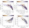 |
Fig. 4. Dust-to-stellar mass ratio, and HI-to-stellar mass ratio as a function of light-weighted age (top). Blue and red solid curves show fit to sub-samples with and without the inflow, respectively. The black dotted line is the fit to the ETGs, the same as in Fig. 2. Hot-to-cold gas mass ratio as a function of age (bottom-left). Specific SFR as a function of age (bottom-right). Solid and dashed lines show |


In Fig. 4, we also show blue (red) contours to denote galaxies with (without) an inflow between this and the previous snapshot. These constitute a total of 18% (82%) of our ETG sample. The AGN radio-mode feedback is responsible for preventing the hot halo gas from cooling down and inflowing into the galaxy. We estimated the dust and HI removal timescales for both sub-samples. We find that galaxies with inflow have longer (shorter) dust (HI) removal timescales as compared to the sub-sample without inflows (although consistent within the errors). Galaxies with inflow are younger with more dust and cold gas [mean log(age/yr) = 9.4, log(Mdust/M⊙) = 7.43, and log(Mcold/M⊙) = 9.7] than galaxies without inflow [mean log(age/yr) = 9.7, log(Mdust/M⊙) = 7.35, and log(Mcold/M⊙) = 9.5]. The sub-sample without inflows shows removal timescales that are in agreement with the timescales estimated for the full sample (for both mass ratios). Thus, the inclusion of the galaxies with inflow does not alter the overall results on dust and gas removal timescales. The bottom-left panel shows the clearest separation between these two sub-samples. Galaxies with inflow show a larger content of cold gas, while galaxies without inflow have much more hot gas. To further investigate this issue, in the bottom-right panel of Fig. 4, we show sSFR as a function of age with the contours representing the same sub-samples as in the rest of the panels. Galaxies without inflow and higher BH masses (colour-coded) are found mostly below the quenched galaxy sSFR limit of  (or below the MS), while galaxies with inflow are above the SFG limit of
  (Rodríguez Montero et al. 2019) (or on the MS), where tH is the Hubble time.
3.3. ISM removal timescales in individual galaxies
By taking advantage of the simulations, it is possible to trace the selected galaxies backwards in time. This allows us to trace the evolution of an individual galaxy and its progenitors. Figure 5 shows the exponential fits to the ISM-to-stellar ratio versus age (described in Sect. 3.1) together with selected fits to the ISM-to-stellar ratio versus age for individual galaxies and their progenitors up to z = 1.14. To find out whether these individual fits are similar to the fit for the ETG sample, we estimated the percentage of fits that have relative errors of the timescale τ lower than 100%. In this way, we were able to select a total of 63% (dust-to-stellar) and 47% (H I-to-stellar mass ratio) of the total ETG sample. The fits failing to meet this criterion correspond to objects with high ISM variations (e.g. due to mergers, see below). These fits are mostly either shallower (i.e. with much larger, unrealistic τ) or significantly steeper (i.e. with much smaller τ).
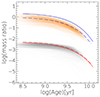 |
Fig. 5. HI-to-stellar and dust-to-stellar mass ratios as a function of light-weighted stellar age. Thin lines show exponential fits to our individual ETG for our sample and their progenitors from which we select fits that have τ/τerr > 1 and these constitute 63% and 47% of the total for the dust- and HI-to-stellar ratios, respectively. Blue and red lines are the same as in Fig. 2. |
It is important to point out that the specific characteristic parameters of the progenitors can significantly differ from the selected early-type descendent galaxy. This is especially true before a merger or disc instability occurs during the evolution of a particular galaxy. In other words, the progenitors of our galaxies might not be early-type galaxies after all (as identified through the selection process described in Sect. 2.3). However, we find that for ∼47−63% of the sample this does not have an impact on the fitting process and we can describe the dust-to-stellar and HI-to-stellar mass ratio evolution with our method at least down to light-weighted age of 108.5 yr.
3.4. Dust and star formation
A strong correlation between dust content and star formation for MS galaxies was found more than a decade ago (da Cunha et al. 2010). A similar, albeit with a lower slope, relation for elliptical galaxies below the MS was first found by Hjorth et al. (2014) and this was recently confirmed using a larger sample in Leśniewska et al. (2023). In particular, Hjorth et al. (2014) analyzed analytical models of dust production and star formation and interpreted the positions of particular populations of galaxies as evolutionary stages (starburst, star formation, and quenched star formation). They suggested that the initial phase is starburst-driven as a result of an increased supply of gas for star formation (e.g. by a merger). In this phase, while the SFR is high, the dust mass is built up quickly. After this phase, a normal star formation takes place which is characterised by a joint decay in dust mass and SFR resulting in the da Cunha et al. (2010) relation. This particular evolutionary phase is described with a slope of ∼1 (found in this work, see below, or 0.9 in Hjorth et al. 2014). This phase is related to the global Schmidt–Kennicutt relation; however, this relation has a larger slope: between 1.2−1.5 (Schmidt 1959; Kennicutt 1998). The last phase is the quenching of star formation in which a rapid decline in SFR is observed, while the dust decline is slower. Taking advantage of the present simulations, here we show how individual galaxies move around this diagram.
In Fig. 6, we show the simulated galaxies and compare them to the observational results (da Cunha et al. 2010; Leśniewska et al. 2023). To this end, we applied a specific sample selection of starburst galaxies (SBGs), normal SFGs, and quenched ETGs below the MS. The majority of the galaxies studied in da Cunha et al. (2010) are normal MS galaxies with late-type morphologies in a similar redshift range to the one used in this work. Thus, we selected galaxies with bulge-to-total mass ratio below 0.3, above the dust mass limit (see the right panel in Fig. 1) and with the same redshift limit as described in Sect. 2.3. These constitute the MS LTG sample. In the context of this particular relation, Leśniewska et al. (2023) studied ETGs divided between galaxies on the MS and below the MS. Thus, in addition to the already described criteria (Sect. 2.3), we also selected galaxies that are below −0.2 dex from the simulated MS (Fig. 1, left panel). While this MS has a steeper slope than the one used in Leśniewska et al. (2023), we can see that both are consistent in the stellar mass range considered in this work. In this way, we selected 68% of the ETG sample below the MS and used it in this exercise.
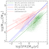 |
Fig. 6. Dust mass as a function of the SFR. The colours of the contours, lines, and points correspond to: ETGs (red), MS LTGs (blue), and SBGs (green). Power-law fits are described as log(Mdust) = a × log(SFR)+b with coefficients given in the legend. Red and blue dotted lines show fits from Leśniewska et al. (2023) and da Cunha et al. (2010), respectively. Individual MS LTG are not shown for the sake of clarity. |
The relation between dust mass and SFR for MS LTG agrees with the observed relation from da Cunha et al. (2010) and is described as:

with a 2σ scatter around the fit of 0.24 dex.
In the case of ETGs, the slope of the fit to simulated galaxies (0.638) is similar to the one from the observed galaxies (0.55; Leśniewska et al. 2023), but with a ∼0.3 dex of difference in the normalisation parameter, namely, our ETG sample below the MS have a lower dust content than the observed one. The relation is as follows:

with a 2σ scatter of 0.23 dex.
In Fig. 6, we also included the relation of dust mass and SFR for simulated SBGs (green contours and line). These were selected (i) as galaxies that are five times above the simulated MS, (ii) with a dust mass is above the dust mass limit estimated from observations (Fig. 1, right panel), and (iii) in the same redshift range (Sect. 2.3). These objects form a sequence that runs almost parallel with the MS galaxies, described as:

with 2σ scatter of 0.32 dex.
Additionally, we tested whether the relations given above hold upon the selection based on star formation activity. To do this, we selected active (sSFR > 1/tH), and passive (sSFR < 1/tH) galaxies without any selection regarding morphology (i.e. bulge-to-total mass ratio), but maintaining the dust mass limit, stellar mass, and redshift range studied in this work as well as in da Cunha et al. (2010) and Leśniewska et al. (2023). We find excellent agreement with both relations, between the MS LTG and active samples as well as between the ETG and passive samples (see Fig. B.1).
Figure 7 shows the same relation for selected ETGs and their progenitors; namely, we trace the evolution of a particular galaxy backward in time. This allows us to identify any merger event together with the redshift and stellar masses of galaxies involved in that event. We define major (minor) mergers as those with a stellar mass ratio of the merging galaxies less (more) than three. Tracing merger events, we find that 92% of our sample went through at least one (four, on average) minor merger event, while 39% had at least one (two, on average) major merger event since z ∼ 2. Only about 3% of our ETGs sample had no merger events (see Fig. D.1). To put our ETG sample into the broader context of galaxy evolution, we estimated the major and minor merger events for SBGs and MS LTGs. We find that 75% (66%) of SBGs (MS LTG) had minor mergers, 11% (2%) had major mergers, and 22% (38%) had no merger events. Hence, it is more likely to select an ETG that had a major or minor merger at some point in its evolution than a MS LTG or SBGs; however, it is less likely to find an ETG without any merger than to find a SFG with no merger events in the past. Starburst galaxies are in between the ETG and MS LTG samples regarding these fractions.
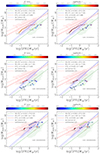 |
Fig. 7. Dust mass as a function of the SFR. Progenitors of the selected ETGs are connected with the lines. Empty red (blue) circles show the progenitor galaxy with a major (minor) merger event before that snapshot. Each row corresponds to one selected ETGs. The left column shows the colour-coded bulge-to-total mass ratio, whereas the right shows the same galaxy but colour-coded by the black hole mass. |
The overall picture found in this work is consistent with the models and interpretation from Hjorth et al. (2014), summarised as follows. Galaxies began to increase their dust mass with a relatively constant (and high) SFR. The merger events alter the SFR, increasing it for a brief time, followed by an equally sharp decrease. Finally, a morphologically changed galaxy (higher bulge-to-total mass ratio) continues its evolution with decreasing SFR and dust mass in the area where quenched (or passive) galaxies are found. These objects also have the most massive black holes (see Fig. B.2). The morphology of galaxies without any merger event is shaped solely by disc instabilities, namely, a mechanism that is efficient enough to drive morphological transformation, as shown in Parente et al. (2023, at least in intermediate-mass galaxies).
3.5. Dust removal mechanisms
Taking advantage of the simulations, it is possible to find the dominant mechanism of dust removal. In particular, we analysed the dust destruction (or removal) rate by SNII and SNIa (SN shocks), the rate of the transition from the cold to hot phase (i.e. ejected from the cold gas as a consequence of the heating from stellar feedback), and astration (the use of cold dust for star formation). These destruction rates are shown in Fig. 8 for our ETG sample, as well as for LTGs and SBGs (for reference). For LTGs and SBGs, the general trends are similar: the shocks from SNII are dominating (by 2−3 dex) over the rest of the mechanisms for the majority of the age span. For ETGs SNII dominate between log(age/yr) ∼ 8.8 and 9.4. After that, stellar feedback dominates, with astration, and SN feedback on a similar level, all decreasing with age. The age range of the change in the main dust destruction and removal mechanism is also aligned with the age at which the feedback from AGN radio mode accretion is strong enough to prevent inflows. Thus, after heating the gas with stellar feedback, the AGN feedback effectively prevents its cooling (see Fig. 4), thereby indirectly decreasing the SFR (and, hence, the SNII rate). Similar result was found in Lorenzon et al. (2024) but using hydrodynamical simulations.
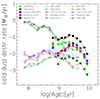 |
Fig. 8. Dust destruction rates as a function of light-weighted age. ETGs, MS LTGs, and SBGs are shown as filled squares, empty circles, and triangles, respectively. Colours denote different destruction and removal mechanisms (see main text for details). Only median values in each age bin are shown for the sake of clarity. |
To test whether some of the destruction mechanism shapes the fitted removal timescale, we switched off each of these at a time. We find that although the normalisation changes by about 0.4 dex, the resulting removal timescales agree with the errors (as shown in Fig. A.1). Our results are consistent with Parente et al. (2023, in particular, as seen in their Fig. 12).
4. Discussion and conclusions
In this work, we adopted the L-GALAXIES2020 SAM (Henriques et al. 2020; Parente et al. 2023) to study the ISM removal timescales in ETGs and compare them with recent observations. We also investigated the relationship between dust mass and SFR. Furthermore, we also investigated the mechanisms that are responsible for the removal or destruction of the cold dust content in simulated galaxies. The selection process involved the observed dust mass limit, thus the results may not be applicable to less dusty ETGs.
Using our selected sample, we recovered the observed ISM (dust and HI) removal timescales (Fig. 1). Our dust and HI removal timescales of τd = 2.28 ± 0.1 and τHI = 1.92 ± 0.09 Gyr are in excellent agreement with τd = 2.26 ± 0.22 and τHI = 1.97 ± 0.10 Gyr estimated for our reference GAMA sample, studied in Leśniewska et al. (2023). We also refer to a similar smaller sample in Michałowski et al. (2024).This confirms that timing the ISM removal using the stellar age is appropriate for these galaxies (as in Michałowski et al. 2019, 2024; Leśniewska et al. 2023).
We show that the dust removal timescale depends slightly on stellar mass and BH mass (albeit at a low statistical significance), with almost identical normalisations with respect to the observationally measured ones. No dependence of the ISM removal on redshift has been found. We do find, however, that using sub-samples divided into stellar mass bins have different normalisation constants (Eq. 1) in the case of the HI-to-stellar mass ratio. This is due to the gas-to-dust mass ratio and its correlation with stellar mass (metallicity), as shown in Rémy-Ruyer et al. (2014, in particular, their Fig. 3). This is also true for BH mass bins, however, it is less visible in the redshift bins.
In the SAM, we used the black hole activity, in particular, the SMBH accretion of hot gas and the consequent radio mode feedback controls the inflow (cooling) of the material. There are 95% (5%) of galaxies with (without) inflow in the MS LTG and SBG samples since the last snapshot. In contrast, we find that 82% of ETGs had no inflow between the current and the previous snapshot. The overall dust and HI removal timescales do not change if we exclude galaxies with inflow (top panels in Fig. 4). The hot-to-cold gas mass ratio is controlled by the black hole activity, increasing with increasing black hole mass (bottom left panel in Fig. 4). Galaxies with higher hot gas masses are also those with low sSFR (or below the MS; see the bottom right panel in Fig. 4). The mechanism that prevents the inflow (radio mode feedback) also retains a galaxy in a passive state, with low SFR, below the MS (as is the case of most of the ETGs). On the other hand, galaxies with inflow are galaxies on and above the MS (as is the case of MS LTGs and SBGs).
Individually, between 63% and 47% of our ETGs and their progenitors follow the dust- and HI-to-stellar mass ratio evolution with time in the same way as the fit for the total sample to the dust- and HI-to-stellar mass ratio with stellar age. The remaining galaxies and their progenitors have increased variations in the dust- and HI-to-stellar mass ratio, which increases the error of the fitting (Fig. 5).
We show that simulated galaxies follow the relation between dust mass and SFR for SFGs on the MS (da Cunha et al. 2010) and for passive ETGs (Hjorth et al. 2014; Leśniewska et al. 2023); the latter exhibit a lower normalisation constant (by about 0.35 dex). To test whether this is due to the excessive dust destruction we investigated the dust-to-gas (DTG) ratio of our sample. We find that the DTG ratio of our ETGs follows the relation between DTG and metallicity for the simulated SFGs (Parente et al. 2023, their Fig. 8) occupying the high DTG and metallicity end of this relation. This indicates that the difference in the normalisation constant is not due to excessive dust destruction, but it is most likely the reflection of the slightly lower stellar and dust masses and SFRs of the selected ETG sample, as compared to the ETGs from Leśniewska et al. (2023, which is explained in Sect. 2.3). We also find, for the first time, a sequence for simulated starburst galaxies, which runs almost parallel to the star-forming galaxies (Fig. 6).
We find that merger events are responsible for the morphological transformation of simulated ETGs. This leads to a bulge mass increase and black hole growth followed by an increase of the radio mode accretion. This accretion mode results in strong feedback which is capable of preventing the hot gas from cooling. Using the relation between dust mass and SFR, we show that a merger event changes dramatically the ISM content, and ignites high star formation. This event is normally followed by steady, and passive evolution of a high bulge-to-total mass ratio galaxy in the regime of passive ETGs (Fig. 7).
Only about 3% of the ETG sample had no mergers in the past. Instead, disc instabilities have played the main role in the morphological transformation of these objects. In Fig. D.1, we show examples of these ETGs and their progenitors. On the other hand, a total of 22% (38%) of SBGs (MS LTGs) had no merger events. This is a considerably higher rate compared to ETGs. This reflects an earlier evolutionary stage, where disc instabilities shape the morphology before the merger-driven morphological transformation occurs.
We investigated different mechanisms of dust destruction implemented in the adopted SAM. Shocks associated with SN explosions dominate the destruction rate over a majority of the galaxy evolution in the MS LTGs, SBGs, and younger ETGs with log(age/yr) < 9.4. For ETGs with log(age) > 9.4, AGN feedback is strong enough to prevent any inflow from the hot gas atmosphere (no cooling), thus slowing down star formation. Then, stellar feedback begins to dominate the dust destruction, while astration and destruction by SNII shock waves are on a similar level (see Fig. 8).
We conclude that SNII-driven destruction dominates in the early stages of ETG evolution. At later stages, the stellar feedback and astration became similarly important, while the AGN feedback prevents the inflow of cool gas, decreasing SFRs. In this scenario, the morphological transformation (mostly merger-driven) is important for efficient BH growth and an increase of AGN feedback.
This in-situ SMBH growth channel is not present in the Henriques et al. (2020) SAM, but it has been included in the Parente et al. (2023) version. Recently, Parente et al. (2024) have shown the relevance of this channel, within the context of this SAM.
Acknowledgments
J.N. would like to thank R. Yates for his useful comments regarding the L-GALAXIES2020, and K. Lisiecki for helpful discussions regarding SIMBA simulations. J.N., M.J.M., and A.L. acknowledge the support of the National Science Centre, Poland through the SONATA BIS grant 2018/30/E/ST9/00208. This research was funded in whole or in part by National Science Centre, Poland (grant number: 2021/41/N/ST9/02662). M.J.M. acknowledges the support of the Polish National Agency for Academic Exchange Bekker grant BPN/BEK/2022/1/00110 and the Polish-U.S. Fulbright Commission. AL and JH were supported by a VILLUM FONDEN Investigator grant (project number 16599). This work was supported by a research grant (VIL54489) from VILLUM FONDEN. For the purpose of Open Access, the author has applied a CC-BY public copyright licence to any Author Accepted Manuscript (AAM) version arising from this submission. The Millennium Simulation databases used in this paper and the web application providing online access to them were constructed as part of the activities of the German Astrophysical Virtual Observatory (GAVO). Authors acknowledge the use of astropy libraries (Astropy Collaboration 2013, 2018), as well as TOPCAT/STILTS software (Taylor 2005). C.G. is supported by a VILLUM FONDEN Young Investigator Grant (project number 25501).
References
- Astropy Collaboration (Robitaille, T. P., et al.) 2013, A&A, 558, A33 [NASA ADS] [CrossRef] [EDP Sciences] [Google Scholar]
- Astropy Collaboration (Price-Whelan, A. M., et al.) 2018, AJ, 156, 123 [Google Scholar]
- Bell, E. F., van der Wel, A., Papovich, C., et al. 2012, ApJ, 753, 167 [CrossRef] [Google Scholar]
- Bianchi, S., & Ferrara, A. 2005, MNRAS, 358, 379 [NASA ADS] [CrossRef] [Google Scholar]
- Bigiel, F., Leroy, A. K., Walter, F., et al. 2011, ApJ, 730, L13 [NASA ADS] [CrossRef] [Google Scholar]
- Chabrier, G. 2003, PASP, 115, 763 [Google Scholar]
- Cheung, E., Faber, S. M., Koo, D. C., et al. 2012, ApJ, 760, 131 [CrossRef] [Google Scholar]
- Clemens, M. S., Jones, A. P., Bressan, A., et al. 2010, A&A, 518, L50 [NASA ADS] [CrossRef] [EDP Sciences] [Google Scholar]
- da Cunha, E., Eminian, C., Charlot, S., & Blaizot, J. 2010, MNRAS, 403, 1894 [Google Scholar]
- De Lucia, G., & Blaizot, J. 2007, MNRAS, 375, 2 [Google Scholar]
- De Lucia, G., Kauffmann, G., & White, S. D. M. 2004, MNRAS, 349, 1101 [Google Scholar]
- Dekel, A., & Silk, J. 1986, ApJ, 303, 39 [Google Scholar]
- Di Matteo, T., Springel, V., & Hernquist, L. 2005, Nature, 433, 604 [NASA ADS] [CrossRef] [Google Scholar]
- Donevski, D., Lapi, A., Małek, K., et al. 2020, A&A, 644, A144 [NASA ADS] [CrossRef] [EDP Sciences] [Google Scholar]
- Gall, C., & Hjorth, J. 2018, ApJ, 868, 62 [CrossRef] [Google Scholar]
- Gall, C., Hjorth, J., & Andersen, A. C. 2011, A&ARv, 19, 43 [NASA ADS] [CrossRef] [Google Scholar]
- Gao, Y., & Solomon, P. M. 2004, ApJS, 152, 63 [Google Scholar]
- Gebhardt, K., Bender, R., Bower, G., et al. 2000, ApJ, 539, L13 [Google Scholar]
- Gensior, J., Kruijssen, J. M. D., & Keller, B. W. 2020, MNRAS, 495, 199 [NASA ADS] [CrossRef] [Google Scholar]
- Granato, G. L., Ragone-Figueroa, C., Taverna, A., et al. 2021, MNRAS, 503, 511 [NASA ADS] [CrossRef] [Google Scholar]
- Henriques, B. M. B., White, S. D. M., Thomas, P. A., et al. 2015, MNRAS, 451, 2663 [Google Scholar]
- Henriques, B. M. B., White, S. D. M., Thomas, P. A., et al. 2017, MNRAS, 469, 2626 [Google Scholar]
- Henriques, B. M. B., Yates, R. M., Fu, J., et al. 2020, MNRAS, 491, 5795 [NASA ADS] [CrossRef] [Google Scholar]
- Herpich, F., Stasińska, G., Mateus, A., Vale Asari, N., & Cid Fernandes, R. 2018, MNRAS, 481, 1774 [CrossRef] [Google Scholar]
- Hirashita, H. 2015, MNRAS, 447, 2937 [NASA ADS] [CrossRef] [Google Scholar]
- Hjorth, J., Gall, C., & Michałowski, M. J. 2014, ApJ, 782, L23 [NASA ADS] [CrossRef] [Google Scholar]
- Hopkins, P. F., Kereš, D., Oñorbe, J., et al. 2014, MNRAS, 445, 581 [NASA ADS] [CrossRef] [Google Scholar]
- Jones, A. P. 2004, ASP Conf. Ser., 309, 347 [NASA ADS] [Google Scholar]
- Kennicutt, R. C. 1998, ApJ, 498, 541 [NASA ADS] [CrossRef] [Google Scholar]
- Knapp, G. R., Gunn, J. E., & Wynn-Williams, C. G. 1992, ApJ, 399, 76 [Google Scholar]
- Krumholz, M. R., McKee, C. F., & Tumlinson, J. 2009, ApJ, 693, 216 [NASA ADS] [CrossRef] [Google Scholar]
- Lara-López, M. A., Cepa, J., Bongiovanni, A., et al. 2010, A&A, 521, L53 [CrossRef] [EDP Sciences] [Google Scholar]
- Leroy, A. K., Walter, F., Sandstrom, K., et al. 2013, AJ, 146, 19 [Google Scholar]
- Leśniewska, A., & Michałowski, M. J. 2019, A&A, 624, L13 [Google Scholar]
- Leśniewska, A., Michałowski, M. J., Gall, C., et al. 2023, ApJ, 953, 27 [CrossRef] [Google Scholar]
- López-Sanjuan, C., Le Fèvre, O., Ilbert, O., et al. 2012, A&A, 548, A7 [Google Scholar]
- Lorenzon, G., Donevski, D., Lisiecki, K., et al. 2024, A&A, in press, https://doi.org/10.1051/0004-6361/202450393 [NASA ADS] [CrossRef] [EDP Sciences] [Google Scholar]
- Magdis, G. E., Gobat, R., Valentino, F., et al. 2021, A&A, 647, A33 [NASA ADS] [CrossRef] [EDP Sciences] [Google Scholar]
- Magorrian, J., Tremaine, S., Richstone, D., et al. 1998, AJ, 115, 2285 [Google Scholar]
- Man, A., & Belli, S. 2018, Nat. Astron., 2, 695 [NASA ADS] [CrossRef] [Google Scholar]
- Martig, M., Bournaud, F., Teyssier, R., & Dekel, A. 2009, ApJ, 707, 250 [Google Scholar]
- Matsuura, M., Dwek, E., Meixner, M., et al. 2011, Science, 333, 1258 [NASA ADS] [CrossRef] [Google Scholar]
- McConnell, N. J., & Ma, C.-P. 2013, ApJ, 764, 184 [Google Scholar]
- Michałowski, M. J. 2015, A&A, 577, A80 [NASA ADS] [CrossRef] [EDP Sciences] [Google Scholar]
- Michałowski, M. J., Murphy, E. J., Hjorth, J., et al. 2010, A&A, 522, A15 [NASA ADS] [CrossRef] [EDP Sciences] [Google Scholar]
- Michałowski, M. J., Hjorth, J., Gall, C., et al. 2019, A&A, 632, A43 [NASA ADS] [CrossRef] [EDP Sciences] [Google Scholar]
- Michałowski, M. J., Gall, C., Hjorth, J., et al. 2024, ApJ, 964, 129 [CrossRef] [Google Scholar]
- Morgan, H. L., & Edmunds, M. G. 2003, MNRAS, 343, 427 [CrossRef] [Google Scholar]
- Mowla, L. A., van Dokkum, P., Brammer, G. B., et al. 2019, ApJ, 880, 57 [NASA ADS] [CrossRef] [Google Scholar]
- Muratov, A. L., Kereš, D., Faucher-Giguère, C.-A., et al. 2015, MNRAS, 454, 2691 [NASA ADS] [CrossRef] [Google Scholar]
- Naab, T., Khochfar, S., & Burkert, A. 2006, ApJ, 636, L81 [NASA ADS] [CrossRef] [Google Scholar]
- Nadolny, J., Lara-López, M. A., Cerviño, M., et al. 2020, A&A, 636, A84 [NASA ADS] [CrossRef] [EDP Sciences] [Google Scholar]
- Nadolny, J., Bongiovanni, Á., Cepa, J., et al. 2021, A&A, 647, A89 [NASA ADS] [CrossRef] [EDP Sciences] [Google Scholar]
- Nadolny, J., Michałowski, M. J., Rizzo, J. R., et al. 2023, ApJ, 952, 125 [NASA ADS] [CrossRef] [Google Scholar]
- Nanni, A., Bressan, A., Marigo, P., & Girardi, L. 2013, MNRAS, 434, 2390 [NASA ADS] [CrossRef] [Google Scholar]
- Parente, M., Ragone-Figueroa, C., Granato, G. L., et al. 2022, MNRAS, 515, 2053 [NASA ADS] [CrossRef] [Google Scholar]
- Parente, M., Ragone-Figueroa, C., Granato, G. L., & Lapi, A. 2023, MNRAS, 521, 6105 [NASA ADS] [CrossRef] [Google Scholar]
- Parente, M., Ragone-Figueroa, C., López, P., et al. 2024, ApJ, 966, 154 [NASA ADS] [CrossRef] [Google Scholar]
- Peng, Y., Maiolino, R., & Cochrane, R. 2015, Nature, 521, 192 [Google Scholar]
- Pillepich, A., Springel, V., Nelson, D., et al. 2018, MNRAS, 473, 4077 [Google Scholar]
- Piotrowska, J. M., Bluck, A. F. L., Maiolino, R., & Peng, Y. 2022, MNRAS, 512, 1052 [NASA ADS] [CrossRef] [Google Scholar]
- Planck Collaboration XVI. 2014, A&A, 571, A16 [NASA ADS] [CrossRef] [EDP Sciences] [Google Scholar]
- Rémy-Ruyer, A., Madden, S. C., Galliano, F., et al. 2014, A&A, 563, A31 [Google Scholar]
- Rodríguez Montero, F., Davé, R., Wild, V., Anglés-Alcázar, D., & Narayanan, D. 2019, MNRAS, 490, 2139 [CrossRef] [Google Scholar]
- Schawinski, K., Urry, C. M., Simmons, B. D., et al. 2014, MNRAS, 440, 889 [Google Scholar]
- Schaye, J., Crain, R. A., Bower, R. G., et al. 2015, MNRAS, 446, 521 [Google Scholar]
- Schmidt, M. 1959, ApJ, 129, 243 [NASA ADS] [CrossRef] [Google Scholar]
- Scoville, N., Lee, N., Vanden Bout, P., et al. 2017, ApJ, 837, 150 [Google Scholar]
- Segovia Otero, Á., Renaud, F., & Agertz, O. 2022, MNRAS, 516, 2272 [NASA ADS] [CrossRef] [Google Scholar]
- Sérsic, J. L. 1963, Boletin de la Asociacion Argentina de Astronomia La Plata Argentina, 6, 41 [Google Scholar]
- Speagle, J. S., Steinhardt, C. L., Capak, P. L., & Silverman, J. D. 2014, ApJS, 214, 15 [Google Scholar]
- Springel, V., White, S. D. M., Jenkins, A., et al. 2005, Nature, 435, 629 [Google Scholar]
- Taylor, M. B. 2005, ASP Conf. Ser., 347, 29 [Google Scholar]
- van Gorkom, J. H., Knapp, G. R., Ekers, R. D., et al. 1989, AJ, 97, 708 [NASA ADS] [CrossRef] [Google Scholar]
- Vogelsberger, M., Genel, S., Springel, V., et al. 2014, MNRAS, 444, 1518 [Google Scholar]
- Whitaker, K. E., Narayanan, D., Williams, C. C., et al. 2021, ApJ, 922, L30 [NASA ADS] [CrossRef] [Google Scholar]
- Wong, T., & Blitz, L. 2002, ApJ, 569, 157 [CrossRef] [Google Scholar]
- Yates, R. M., Henriques, B., Thomas, P. A., et al. 2013, MNRAS, 435, 3500 [CrossRef] [Google Scholar]
Appendix A: Dust destruction and removal mechanisms
Here, we show the results of the SAM predictions with different dust destruction and ejection mechanisms switched off. In particular, new runs with no SN destruction (noSN), no astration (noAstr), and no ejection from cold gas (noColdHot) were performed. Figure A.1 shows the resulting exponential fits with removal timescales varying between 2.34 and 2.55 [Gyr], this is within 10% of the fiducial model. Thus, the general ISM removal timescale found in used SAM does not depend on the individual removal and ejection mechanisms. Considering the normalisation of the exponential fits, we can see that noSN model gives a very similar dust-to-stellar mass ratio as the fiducial model. In the fiducial model, the gas phase metals produced by the SNe destruction are quickly accreted again into grains by the accretion process. Thus, in the noSN model this does not happen, thus accretion is also reduced and the resulting dust content is roughly similar to the fiducial model. Considering noAstr and noColdHot models, the removal timescale is similar, but the normalisation is higher. This is because the two processes remove the dust (and metals) from the cold gas, while the SNe transfer the dust metals into the gas phase, leaving them available in the cold phase (Parente et al. 2023).
Appendix B: Dust mass and SFR
To test whether our morphologically based selection indeed corresponds to a passive galaxy sample, here we provide a selection based on sSFR. We select active galaxies using sSFR > 1/tH, while passive galaxies are defined as sSFR < 1/tH. Additionally, we also keep the dust mass limit, stellar mass limit and redshift range to be able to make a direct comparison with observations as well as with the results described in Sect. 3.4. As shown in Fig. B.1 the results obtained using sSFR to select active and passive galaxies are similar to the selection based on morphology, with 2σ scatter of 0.23 and 0.26, respectively. The fitting coefficients are given in the legend and we can see that both the slopes and intercepts are in agreement.
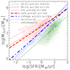 |
Fig. B.1. Dust mass as a function of SFR as a function of BH mass. Colours are the same as in Fig. 6, with additional thick blue and red dashed lines showing a relation for active (sSFR > 1/tH) and passive galaxies respectively (sSFR < 1/tH). |
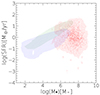 |
Fig. B.2. SFR as a function of BH mass. In blue, green, and red we show SFGs, SBGs, and ETGs. |
Appendix C: SFR and black hole mass
Figure B.2 shows SFRs as a function of BH masses for the MS LTGs, SBGs, and ETGs. The most massive BHs are found in simulated ETGs. The growth of the bulge in a galaxy is likely followed by the BH mass growth.
Appendix D: SFR and dust masses for galaxies without a merger event
In Fig. D.1, we show examples of simulated ETGs from our sample that did not go through a merger event during its evolution. These constitute ∼3% of the sample. Their morphological transformation was driven by disc instabilities as implemented in the SMA used in this work. For details, see Parente et al. (2023).
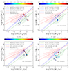 |
Fig. D.1. Same as Fig. 7 but for galaxies without a merger event during their evolution. The bulge-to-total mass ratio is colour-coded. |
All Figures
|
Fig. 1. SFR as a function of stellar mass (left). The solid line shows the MS from the L-GALAXIES2020 simulations estimated using LTGs (see main text for details) and is a power-law fit described as log(SFR) = a × log(M*)+b with coefficients given in the legend. The dotted line shows the MS estimated using a prescription from Speagle et al. (2014), both at z = 0.18. Orange and gray points show the GAMA, and L-GALAXIES2020 ETG samples. Normalised stellar mass distribution for the mentioned samples (top). Dust mass as a function of redshift (right). The dashed line shows the dust mass limit estimated for the GAMA sample. More details are given in Sect. 2.3. |
| In the text | |
|
Fig. 2. HI-to-stellar and dust-to-stellar mass ratios as a function of light-weighted stellar age. Exponential fits to L-GALAXIES2020 ETG samples (dashed lines), together with observationally derived fits from Michałowski et al. (2024), Leśniewska et al. (2023) (continuous and dotted lines) are shown. |
| In the text | |
|
Fig. 3. HI-to-stellar and dust-to-stellar mass ratio as a function of light-weighted age. Orange and grey lines show fits to HI- and dust-to-stellar mass ratios for sub-samples divided into stellar mass (top row), the black hole-to-stellar mass ratio (middle), and redshift (bottom row) bins. Blue and red dashed lines show fits to the overall ETG sample from Fig. 2 and are given for reference. |
| In the text | |
|
Fig. 4. Dust-to-stellar mass ratio, and HI-to-stellar mass ratio as a function of light-weighted age (top). Blue and red solid curves show fit to sub-samples with and without the inflow, respectively. The black dotted line is the fit to the ETGs, the same as in Fig. 2. Hot-to-cold gas mass ratio as a function of age (bottom-left). Specific SFR as a function of age (bottom-right). Solid and dashed lines show |
| In the text | |
|
Fig. 5. HI-to-stellar and dust-to-stellar mass ratios as a function of light-weighted stellar age. Thin lines show exponential fits to our individual ETG for our sample and their progenitors from which we select fits that have τ/τerr > 1 and these constitute 63% and 47% of the total for the dust- and HI-to-stellar ratios, respectively. Blue and red lines are the same as in Fig. 2. |
| In the text | |
|
Fig. 6. Dust mass as a function of the SFR. The colours of the contours, lines, and points correspond to: ETGs (red), MS LTGs (blue), and SBGs (green). Power-law fits are described as log(Mdust) = a × log(SFR)+b with coefficients given in the legend. Red and blue dotted lines show fits from Leśniewska et al. (2023) and da Cunha et al. (2010), respectively. Individual MS LTG are not shown for the sake of clarity. |
| In the text | |
|
Fig. 7. Dust mass as a function of the SFR. Progenitors of the selected ETGs are connected with the lines. Empty red (blue) circles show the progenitor galaxy with a major (minor) merger event before that snapshot. Each row corresponds to one selected ETGs. The left column shows the colour-coded bulge-to-total mass ratio, whereas the right shows the same galaxy but colour-coded by the black hole mass. |
| In the text | |
|
Fig. 8. Dust destruction rates as a function of light-weighted age. ETGs, MS LTGs, and SBGs are shown as filled squares, empty circles, and triangles, respectively. Colours denote different destruction and removal mechanisms (see main text for details). Only median values in each age bin are shown for the sake of clarity. |
| In the text | |
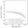 |
Fig. A.1. Same as Fig. 2, but with different dust destruction-and-ejection mechanisms switched off. |
| In the text | |
|
Fig. B.1. Dust mass as a function of SFR as a function of BH mass. Colours are the same as in Fig. 6, with additional thick blue and red dashed lines showing a relation for active (sSFR > 1/tH) and passive galaxies respectively (sSFR < 1/tH). |
| In the text | |
|
Fig. B.2. SFR as a function of BH mass. In blue, green, and red we show SFGs, SBGs, and ETGs. |
| In the text | |
|
Fig. D.1. Same as Fig. 7 but for galaxies without a merger event during their evolution. The bulge-to-total mass ratio is colour-coded. |
| In the text | |
Current usage metrics show cumulative count of Article Views (full-text article views including HTML views, PDF and ePub downloads, according to the available data) and Abstracts Views on Vision4Press platform.
Data correspond to usage on the plateform after 2015. The current usage metrics is available 48-96 hours after online publication and is updated daily on week days.
Initial download of the metrics may take a while.