| Issue |
A&A
Volume 689, September 2024
|
|
|---|---|---|
| Article Number | A225 | |
| Number of page(s) | 16 | |
| Section | Stellar structure and evolution | |
| DOI | https://doi.org/10.1051/0004-6361/202449720 | |
| Published online | 17 September 2024 | |
Optical polarimetry study of the Lambda-Orionis star-forming region
1
Aryabhatta Research Institute of Observational Sciences (ARIES), Nainital 263002, India
2
Indian Institute of Astrophysics (IIA), Sarjapur Road, Koramangala, Bangalore 560034, India
Received:
24
February
2024
Accepted:
20
May
2024
Abstract
We present an optical polarimetry study of the nearby star-forming region Lambda-Orionis to map the plane-of-the-sky magnetic field geometry to understand the magnetized evolution of the HII region and the associated small molecular clouds. We made multiwavelength polarization observations of 34 bright stars distributed across the region. We also present the R-band polarization measurements that focused on the small molecular clouds, bright-rimmed clouds (BRC), BRC 17, and BRC 18, which are located at the periphery of the HII region. The magnetic field lines exhibit a large-scale ordered orientation consistent with the Planck submillimeter polarization measurements. The magnetic field lines in the two BRCs are found to be roughly in north-south directions. However, a larger dispersion is noted in the orientation for BRC 17 compared to BRC 18. Using a structure-function analysis, we estimate the strength of the plane-of-the-sky component of the magnetic field as ∼28 μG for BRC 17 and ∼40 μG for BRC 18. The average dust grain size and the mean value of the total-to-selective extinction ratio (RV) in the HII region are found to be ∼0.51 ± 0.05 μm and ∼2.9 ± 0.3, respectively. The distance of the whole HII region is estimated as ∼392 ± 8 pc by combining astrometry information from Global Astrometric Interferometer for Astrophysics (Gaia) early data release 3 (EDR3) for young stellar objects associated with BRCs and confirmed members of the central cluster Collinder 69.
Key words: techniques: polarimetric / ISM: clouds / ISM: magnetic fields / galaxies: star formation
Corresponding author; This email address is being protected from spambots. You need JavaScript enabled to view it. , This email address is being protected from spambots. You need JavaScript enabled to view it. .
© The Authors 2024
 Open Access article, published by EDP Sciences, under the terms of the Creative Commons Attribution License (https://creativecommons.org/licenses/by/4.0), which permits unrestricted use, distribution, and reproduction in any medium, provided the original work is properly cited.
This article is published in open access under the Subscribe to Open model. This email address is being protected from spambots. You need JavaScript enabled to view it. to support open access publication.
1. Introduction
HII regions are among the most fascinating astronomical objects at optical wavelengths. Several analytical and numerical studies have been conducted to comprehend their formation and expansion (see Arthur et al. 2011; Zamora-Avilés et al. 2019 and reference therein) and to explain the filamentary structures, globules, pillars, clumps, and so on that are found within and around these regions (e.g., Sugitani et al. 1991; Chauhan et al. 2009). These features could be due to the instabilities in the ionization front or to the density inhomogeneities in the molecular cloud inside which the HII region expands (see Garcia-Segura & Franco 1996; Mackey & Lim 2010). Small, isolated, and dense molecular clouds, called bright-rimmed clouds (BRCs), are located at the periphery of the evolved HII regions. When HII regions interact with their surrounding molecular clouds, they form the BRCs. The ultraviolet radiation from the nearby OB stars photoionizes the outer surface layers of a BRC, forming a layer of hot ionized gas known as the ionized boundary layer (IBL). The recombination processes in the IBL result in the formation of optically bright rims. The photoionization-induced shocks are driven into the molecular clouds, forming dense cores that are then triggered to collapse to form new stars (Elmegreen 2011). This phenomenon of triggered star formation by the compression of gas due to shock or an ionization front is known as the radiation-driven implosion (RDI; Bertoldi 1989; Miao et al. 2006) scenario.
The magnetic field plays a very crucial role in the molecular clouds by regulating the star formation processes (see McKee & Ostriker 2007). The expanding HII region and photodissociation region (PDR) tend to remove the preexisting small-scale disordered magnetic field structure and produce a large-scale ordered magnetic field in the neutral shell, with an orientation approximately parallel to the ionization front (Arthur et al. 2011). Soler et al. (2013) found that magnetic field lines are preferentially oriented parallel to most of the density structures and that the relative orientation changes from parallel to perpendicular when the density exceeds a critical density. The strength of the magnetic field decides whether the field lines align themselves along the direction of the ionization radiation or remain unchanged (Henney et al. 2009; Mackey & Lim 2011).
The role of the magnetic field has been investigated in several BRCs using polarimetry. Optical polarimetry studies have shown that the magnetic field could shape the BRCs along with the ionizing radiation from the hot star(s) located in the vicinity of the BRCs (Soam et al. 2017, 2018). The Atacama Large Millimeter/submillimeter Array (ALMA) dust polarization study of NGC 6334 by Cortés et al. (2021) revealed a complex morphology with a significant degree of turbulence, which might be due to the strong interactions between the magnetic field and the turbulent gas in the BRC. Recent submillimeter observations, such as POL-2 on the James Clerk Maxwell Telescope (JCMT), have revealed complex magnetic fields in regions where stars are yet to form (Liu et al. 2019; Pattle et al. 2021).
The Orion molecular cloud complex is a nearby giant molecular cloud complex whose head part is known as the Lambda Orionis star-forming region (LOSFR). It is an ideal location for studying the young stellar population and their environment (Mathieu 2008). The LOSFR is an HII region (Sh2-264, Sharpless 1959) that is illuminated by an O8III-type star called λ-Ori or Meissa, which lies at a distance of 450 ± 50 pc from the Sun (Dolan & Mathieu 1999). Another B0-type main-sequence star forms a binary with Meissa at an angular distance of 4.4″. Zhang et al. (1989) detected a dense molecular gas and dust ring with a diameter of 9° centered around the λ-Ori star using the Infrared Astronomical Satellite (IRAS). This ring coincides with the shell of neutral hydrogen that was previously discovered by Wade (1957). The compact open cluster Collinder 69 is located at the center of the LOSFR, and the λ-Ori star is the brightest member of this cluster. At the periphery of the λ-Ori ring, many dark clouds are located, such as Barnard 30 (B30), Barnard 35 (B35), Barnard 36 (B36), and Barnard 224 (B224). They were cataloged by Barnard (1919). B30 and B35 are also called BRC 17 or SFO 17 and BRC 18 or SFO 18, respectively. They were cataloged by Sugitani et al. (1991). BRC 17 is located at the northwest edge and is separated from λ-Ori by ∼2°, and the elongated BRC 18 cloud projects inward from the eastern edge at an angular distance of ∼2.5° from λ-Ori.
The λ-Ori regions have been extensively studied in various aspects, such as the initial discovery, the distance of the clouds, an Hα survey, an analysis of IRAS data, and photometric and spectroscopic studies. Duerr et al. (1982) performed an Hα survey and identified emission line sources that are predominantly distributed near the open cluster Collinder 69 and the two dark clouds BRC 17 and BRC 18. Dolan & Mathieu (1999, 2001, 2002) studied the whole LOSFR using a lithium survey and deep VRI photometry. They concluded that young stars are spatially distributed around λ-Ori and in front of BRC 17 and BRC 18. However, some young stars are found outside these high stellar-density clouds. It was therefore proposed that the star formation was centered in an elongated cloud extending from BRC 18 through λ-Ori to the BRC 17 cloud (Dolan & Mathieu 1999). The LOSFR comprises recently formed stars from 0.2 M⊙ to 24 M⊙, and star formation still continues in the dark clouds BRC 17 and BRC 18 (Mathieu 2008).
The magnetic field morphology in λ-Ori region will provide useful information about the expansion and evolution of LOSFR and the globules associated with this region. In this paper, we map the global magnetic field geometry in multiple wavelengths and the local magnetic field geometry in BRC 17 and BRC 18 in the R band. The structure of this paper is as follows: in Sect. 2, we briefly describe the optical polarimetry observations and data reduction. Our results and analyses are presented in Sect. 3, followed by a discussion in Sect. 4. We present a summary and highlight our main findings in Sect. 5.
2. Observation and data reduction
We performed the optical linear polarization observations of the LOSFR containing BRC 17 and BRC 18 using the ARIES IMaging POLarimeter (AIMPOL) mounted at the 104 cm Sampurnanand telescope, which is situated at the Aryabhatta Research Institute of Observational Sciences (ARIES), Nainital, India. We used standard Johnson VRI filters with λVeff = 0.550 μm, λReff = 0.670 μm, and λIeff = 0.805 μm for the polarimetric observations. A detailed description of AIMPOL and the polarization measurement methods is given in Ramaprakash et al. (1998), Rautela et al. (2004). The steps of the data reduction methods are described in previous papers (e.g., Eswaraiah et al. 2011, 2012, 2013; Neha et al. 2016, 2018; Soam et al. 2013, 2015, 2017; Soam et al. 2018). The observations were performed between 2014 and 2016. The details of the observations are given in the Table 1. We have observed the stars that are brighter than 15 magnitudes in the V band toward each region in LOSFR.
Log of observations.
Unpolarized standard stars were observed during every run to check for any possible instrumental polarization. The instrumental polarization is found to be lower than 0.1%. We corrected the observed degree of polarization for the instrumental polarization. The reference direction of the polarizer was determined by observing polarized standard stars from Schmidt et al. (1992). We observed these unpolarized and polarized standards using the standard Johnson VRI filters. Schmidt et al. (1992) used the standard Johnson V filter and the Kron-Cousins R and I filters to observe the standard stars. We used the offset between the standard polarization position angle values estimated from the observations and those taken from Schmidt et al. (1992) to correct for the zero point offset. The zero point offset values for the polarization position angles range from 6° to 9° for all the observations.
3. Results and analyses
3.1. Distance to the LOSFR
We have used Global Astrometric Interferometer for Astrophysics (Gaia) early data release 3 (EDR3) data to estimate the distance of LOSFR (Gaia Collaboration 2021). We separately estimated the distances toward BRC 17, BRC 18, and the central cluster Collinder 69. The detailed distance estimation for BRC 18 is presented in Saha et al. (2022). In the case of BRC 17, we compiled a list of YSOs from literature using the criterion given in Saha et al. (2022). We selected candidate YSOs toward BRC 17 within a circular region of 0.5° radius around the IRAS sources (Dolan & Mathieu 2001; Hayashi et al. 2012; Koenig et al. 2015; Kounkel et al. 2018; Zari et al. 2018; Hosoya et al. 2019). In the case of Collinder 69, we selected probable cluster members (Bayo et al. 2012). After compiling all the sources, we searched for each source within a search radius of 1″ and obtained the distance and the proper motion in right ascension and declination from Bailer-Jones et al. (2021) and from the Gaia EDR3 archive (Gaia Collaboration 2021). We selected sources with a ratio, x/Δx ≥ 3, where x represents the distance (d), the proper motion in right ascension (μα) and declination (μδ) values, and Δx shows their respective errors. We also applied the condition for renormalized unit weight errors (RUWE; Lindegren 2018; Lindegren et al. 2021) for all the sources. We selected the sources with RUWE ≤ 1.4 and confirmed their authentic astrometric measurements (Lindegren 2018). The ionizing source λ-Ori for LOSFR is located in the central cluster Collinder 69. The distance of λ-Ori is estimated at 386 ± 60 pc using Gaia EDR3 parallax measurements, but the RUWE is found to be 4.823, which is much higher than the cutoff value of 1.4 (Gaia Collaboration 2021). Hence, we used all the probable cluster members to estimate the distance of Collinder 69 and assigned the same distance to λ-Ori.
Fig. 1 represents μα and μδ of the candidate YSOs associated with BRC 17 and the known cluster members associated with Collinder 69 as a function of their distances (d). We estimated the median absolute deviation (MAD) to measure the statistical dispersion in the datasets because the standard deviations are generally affected by extreme values. We identified the sources lying within 5 × MAD of the median values of the distance and the proper motions for BRC 17 and Collinder 69. The distance uncertainties of individual sources were not considered when we calculated the median distance. After applying this condition, we excluded outliers and estimated the median and MAD values only for the sources that met this condition. The medians with their respective MAD values for μα, μδ and d are listed in Table 2 for BRC 17, BRC 18, and Collinder 69. The distances toward all three different regions of LOSFR are found to be consistent within the error limits. We, therefore, took the mean values of all three distance values to assign a single distance for the LOSFR. The mean distance is 392 ± 8 pc for the LOSFR.
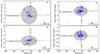 |
Fig. 1. Proper motion values of the known candidate YSOs associated with BRC 17 (left panel) and the known probable cluster members associated with Collinder 69 (right panel) plotted as a function of their distances obtained from Gaia EDR3. Panels a and c: μα vs. d plot of the sources. The candidate YSOs and cluster members lying within a 5 × MAD boundary in the μα vs. d plot are plotted using filled blue circles, and the outliers are plotted using open gray circles. The dashed lines indicate the median values of μα and d of the candidate YSOs and cluster members. Panels b and d: μδ vs. d plot of the sources. The gray shaded ellipses show the 5 × MAD boundary range in distance and proper motions within which the sources are used to estimate a distance. The candidate YSOs and cluster members lying within the 5 × MAD boundary in the μδ vs. d plot are plotted using filled blue circles, and the outliers are plotted using open gray circles. The dashed lines indicate the median values of d and μδ of the candidate YSOs and cluster members. |
Medians with their respective MAD values for μα, μδ, and d.
Murdin & Penston (1977) estimated the distance of the LOSFR using high-quality broadband photometry of the 11 OB stars located at the center of the star-forming region. They estimated the distance of this region to be ∼400 pc. The distance of the five stars in the central area of LOSFR is ∼380 ± 30 pc (Perryman et al. 1997). Dolan & Mathieu (2001) used Strömgren photometry with a larger sample of OB stars and estimated the distance of the region as ∼450 ± 50 pc, which is slightly larger than the previously estimated distances. Recently, Kounkel et al. (2018) estimated the distances for BRC 17 as 397 ± 4 pc, BRC 18 as 396 ± 4 pc and Collinder 69 as 404 ± 4 pc using Gaia DR2 parallax measurements. Our estimated distances for BRC 17 and BRC 18 are consistent within the error limits, but there is a small difference in the distance of Collinder 69. The reason might be that we used the recent Gaia EDR3 distance measurements, whose uncertainties are very low.
3.2. Polarimetry
3.2.1. Foreground polarization subtraction
The distance of the LOSFR was found to be 392 ± 8 pc as described in Section 3.1. Hence, the polarization measurements for the stars towards LOSFR could be affected by the line-of-sight foreground interstellar component. To remove the foreground contribution, we searched BRC 17 and BRC 18 within a circular region with a diameter of 1° for stars with parallax measurements by the HIPPARCOS satellite in van Leeuwen (2007) because the Gaia datasets were not available at the time of these observations. Stars that are found to be the emission line sources in binary or multiple systems or peculiar sources in SIMBAD were excluded. We chose stars with parallax measurements better than 2σ. The polarization observations of these stars were carried out using AIMPOL. We also chose the stars from Heiles catalog (Heiles 2000) within a radius of 4.5° of the λ-Ori region. The polarization results for these stars are presented in Table 3 according to their increasing distance from the Sun. The observed R-band polarization values are presented for BRC 17 and BRC 18, while the values from the Heiles (2000) catalog are the average values in multiple bands as taken directly from the catalog. We also adopted the distances for all the sources from Bailer-Jones et al. (2021) to compare them with previously known distances. We plot the degree of polarization and the polarization angles with distance for all the foreground stars in Fig. 2. In the same figure, we also include the polarization measurements for the bright Tycho stars (Høg et al. 2000, discussed in Section 3.2.2) that lie behind the cloud. The figure shows that the values of the polarization angle are random for stars that lie before 392 pc, but the values are aligned in a particular direction after 392 pc. Similarly, the value of the degree of polarization also increases at about 392 pc, which is consistent with our measured distance. Hence, we calculated the mean values of P and θ for the foreground stars with a distance smaller than 392 pc according to a new distance estimation method (Bailer-Jones et al. 2021) and stars with polarization values greater than 0.1%, which is equal to the instrumental polarization of AIMPOL. We mark these objects with asterisks. The observed foreground R-band polarization values were converted into V band and I band using the Serkowski law (Serkowski et al. 1975). The mean values of the P and θ are 0.3 ± 0.1% and 106 ± 9° for all the V, R, and I filters. Using these mean polarization values, we calculated the Stokes parameters Qfg and Ufg for the selected foreground stars. We also computed the Stokes parameters for our observed stars Q* and U*. Then, we calculated the foreground-corrected Stokes parameters for our observed stars Qc and Uc using Qc = Q* − Qfg and Uc = U* − Ufg, following the same procedure as described in Neha et al. (2016). However, the mean of the difference between observed polarization angles θobserved and the foreground-corrected polarization angles θc is 4° with a standard deviation of 4°, suggesting a smaller contribution due to the foreground. We present the polarization position angle values in the equatorial coordinate system.
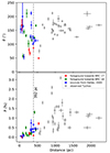 |
Fig. 2. Polarization angle vs. distance of the foreground stars found within a diameter of 1° around BRC 17, BRC 18, and the Heiles stars found within a diameter of 9° around λ-Ori (upper panel). Degree of polarization vs. distance for the same stars (lower panel). The dashed gray line corresponds to a distance of 392 pc in both panels. The distances are calculated from the HIPPARCOS parallax measurements taken from van Leeuwen (2007) and adopted from Bailer-Jones et al. (2021). The gray circles show the bright Tycho stars behind the cloud. The distances for the Tycho stars are taken from Bailer-Jones et al. (2021). |
Polarization values of the observed foreground stars and from the Heiles catalog.
3.2.2. Global magnetic field geometry of LOSFR
We systematically made the polarization study to map the global magnetic field in the LOSFR by observing the bright Tycho stars located behind this region. We selected the bright Tycho stars from the Tycho-2 catalog (Høg et al. 2000) within a radius of 4.5° around λ-Ori. Then, we took the J, H, and Ks magnitudes of these stars from the 2MASS point source catalog (Cutri et al. 2003). We plotted their J, H, and Ks magnitudes in a color-color diagram and selected the stars with J − Ks > 1, showing the stars are reddened or behind the cloud. We made multiband polarimetric observations of 34 of these bright Tycho stars that are distributed in the whole HII region. We also obtained the distances for all these 34 bright Tycho stars from Bailer-Jones et al. (2021) and found that their distances exceed the LOSFR distance (400 pc adopted from the literature). This suggests that our method of selecting the reddened stars is reliable. We plot the polarization vectors in the Planck 857 GHz image in Fig. 3 for the V, R, and I filters from top to bottom. The direction of the polarization vectors shows the global magnetic field geometry in LOSFR, which seems to follow the large-scale structure seen in all the images of Fig. 3. However, the number of stars in our sample is low. Observations of more stars would, therefore, be helpful. The magnetic field lines appear almost parallel to the Galactic plane (b = −11.99°) in the northeast and central regions of LOSFR, while in the southwest region, the field lines seem random. The polarization results for all the Tycho stars toward LOSFR in the VRI filters are given in Table A.1. The mean values of the degree of polarization and the polarization angle for these bright Tycho stars are 1.3 ± 0.2% and 169 ± 6° for the V band, 1.1 ± 0.1% and 163 ± 6° for the R band, and 1.0 ± 0.1% and 170 ± 6° for the I band.
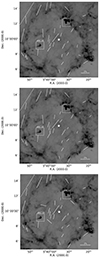 |
Fig. 3. Polarization vectors of 34 bright Tycho stars plotted in the Planck 857 GHz image of LOSFR in the V band (upper panel), R band (middle panel), and I band (lower panel). The length of the vectors corresponds to the degree of the polarization values, while the orientation represents the polarization angle measured from north to east. A vector with a polarization of 2% is shown for reference. The dashed white line shows the position of the Galactic plane. The white star shows the position of λ-Ori. |
3.3. Dust grain size distribution
The Serkowski law (Serkowski et al. 1975) with the parameter K provides an appropriate description of the interstellar polarization with the wavelength in the visible region, and it is defined as follows:
![Mathematical equation: $$ \begin{aligned} {P_\lambda = P_{\rm max}\,\exp [-K\,\ln ^2(\lambda _{\rm max}/\lambda )]}, \end{aligned} $$](/articles/aa/full_html/2024/09/aa49720-24/aa49720-24-eq1.gif) (1)
(1)
where Pλ is the degree of polarization (%) at wavelength λ, Pmax is the maximum degree of polarization estimated from the fitting at wavelength λmax, and the parameter K determines the width of the peak in the curve and was adopted as K = 1.15 (Serkowski et al. 1975). If the polarization is produced by aligned interstellar dust grains, the observed data follow Eq. (1) and the values of Pmax and λmax for each star can be calculated. We studied the dust properties of LOSFR by obtaining the Pmax and λmax values using the weighted least-squares fitting to the measured polarization in the V, R, and I bands.
The λmax values can also be used to infer the origin of the polarization. Stars whose λmax is much lower than the average value of the interstellar medium (0.55 μm; Serkowski et al. 1975) may have an intrinsic component of polarization due to the scattering process (Orsatti et al. 1998). Fig. 4 shows the Serkwoski fitting for 34 stars for which we obtained λmax values between 0.37 μm to 0.66 μm. The weighted mean values of the Pmax and λmax for 34 stars are found to be 1.30 ± 0.11% and 0.51 ± 0.05 μm. Since we only observed at three wavelength bands (VRI), we investigated the effect of using only three wavelength bands on the measured Pmax and λmax. To do this, we compiled the polarimetric data of some randomly selected clouds, that is, NGC 5617, NGC 5749 in UBVRI and LDN 1570, and NGC 457 in BVRI filters from Orsatti et al. (2010), Vergne et al. (2007), Eswaraiah et al. (2013), and Topasna et al. (2017), respectively, and estimated the values of Pmax and λmax by reducing the number of wavelength bands, that is, using the UBVRI, BVRI, and VRI filters. The mean values of λmax and Pmax for these three regions are shown in Table 4. Using the BVRI dataset, the mean values of λmax and Pmax for NGC 5749 are found to be 0.60 ± 0.05 μm and 1.61 ± 0.08%, while using the VRI filters alone, the values are found to be 0.69 ± 0.07 μm and 1.59 ± 0.07%. Similarly, the mean values of λmax and Pmax for LDN 1570 are found to be 0.61 ± 0.04 μm and 2.90 ± 0.11% from the BVRI dataset and 0.63 ± 0.07 μm and 2.85 ± 0.15% from the VRI dataset. We found that the values of λmax for the VRI dataset are consistent within the uncertainty compared with the UBVRI and BVRI datasets. The difference in the λmax and Pmax values in different filter sets is within 10%. This shows that our results can be used to estimate the dust grain size in LOSFR. The estimated λmax is 0.51 ± 0.05 μm, which is consistent with the value corresponding to the general interstellar medium (0.55 μm; Serkowski et al. 1975). It is also consistent with a value 0.53 μm for LOSFR along the Galactic plane estimated from the empirical relation, λmax = 0.545 + 0.030 sin(l + 175°) (Whittet 1977). This relation describes the systematic modulation of λmax as a function of Galactic latitude (l). We also estimated the value of RV, the total to selective extinction, using the relation RV = (5.6 ± 0.3) × λmax (Whittet & van Breda 1978) for all the 34 stars. The RV values range from 1.96 to 3.70 for all 34 Tycho stars. The mean value of RV for these 34 stars is 2.9 ± 0.3, which agrees with the general average value (RV = 3.1) for the Milky Way galaxy within the error limits, indicating that the size of the dust grains within the LOSFR is normal.
 |
Fig. 4. Serkowski curve for 34 bright Tycho stars observed in the VRI filters. The filled blue, green, and red circles correspond to the V, R, and I bands, respectively. The solid magenta line represents the fitting using the Serkowski law (Serkowski et al. 1975). |
Mean values of λmax and Pmax for the UBVRI, BVRI, and VRI dataset for various regions.
3.4. Magnetic field geometry of BRC 17 and BRC 18
The magnetic field geometry of a molecular cloud is predominantly regulated by the relative dynamical importance of the magnetic forces for gravity, turbulence, and thermal pressure. If the magnetic field lines strongly support the molecular cloud against gravity, then the magnetic field lines would be aligned smoothly. The average magnetic field orientation would be perpendicular to the major axis of the cloud (Mouschovias 1978). The cloud tends to shrink more in the parallel direction to the magnetic field than in the perpendicular direction. However, if turbulence is stronger than the magnetic field, then the structural dynamics of the molecular cloud would be controlled by the random motions, and the turbulent eddies will drag the magnetic field lines around (Ballesteros-Paredes et al. 1999). Thus, the magnetic field lines would become chaotic without a preferred direction.
The results of our optical polarimetry observations of 105 stars in the direction of BRC 17 and 171 stars toward BRC 18 are presented in Table A.2. We only list the results of the sources with a degree of polarization measurements better than 2σ. The columns of these tables show the star identification number in increasing order of their right ascension, the declination, the measured P (%), and the polarization position angles (θ in degrees).
3.4.1. BRC 17
The cloud complex B30 contains the Barnard clouds B31 and B32 and the Lynds clouds LDN1580−1584 (Dolan & Mathieu 2001). At the head part of this cloud, a visible bright rim is present, and this is cataloged as BRC 17 by Sugitani et al. (1991). The distance to BRC 17 is estimated at around 389 ± 9 pc (see Section 3.1). The projected angular distance of BRC 17 from the ionizing star λ-Ori is ∼2.3°, which corresponds to ∼15 pc considering the cloud distance 389 pc. Zhou et al. (1988) mapped this cloud using CO observations and divided it into two parts: The northern part, containing the RNO 43 outflow, and the southern part, containing the bright-rim and IRAS source. We mapped the magnetic field geometry toward the southern region, which contains the bright rim of this cloud. The left panel of Fig. 5 shows the plot of the polarization vectors of 105 foreground-subtracted stars overplotted on the WISE 12 μm image. The length and orientation of the vectors correspond to the measured P% and θ values, respectively. The θ is measured from the north, increasing toward the east. The dashed white line represents the orientation of the Galactic plane at the Galactic latitude of −11.6°. The mean values of the degree of polarization and polarization angle for BRC 17 are 1.4 ± 0.4% and 175 ± 43°, respectively. The plot of P% versus θ and the histogram of the θ after correcting for the foreground interstellar contribution are shown in Fig. 6. At first, we performed a single Gaussian fit to the histogram with a bin size of 10 deg. The mean and standard deviation of the best-fit Gaussian is found to be 172 ± 9 deg and 52 ± 12 deg, respectively. The distribution of the polarization position angle appears to be a mixture of multiple Gaussians with the strongest central peak. Therefore, we also fit a multiple Gaussian model of three Gaussians to the data. The multi-Gaussian model shows the strongest peak at the center, with a mean and standard deviation of 167 ± 14 deg and 24 ± 19 deg, respectively. Although the different peaks in the multi-Gaussian model are not well separated, and the parameters are not well constrained and have large uncertainties, we find a similar reduced χ2 as that of the single-Gaussian model. However, the standard deviation value of the central Gaussian in the multi-Gaussian model is much lower than the single Gaussian model.
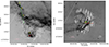 |
Fig. 5. Polarization vectors overplotted on the WISE 12 μm image of BRC 17 (left panel) and BRC 18 (right panel). The length of the vectors corresponds to the degree of polarization, and the orientation corresponds to the position angle measured from the north and increasing toward the east. A vector corresponding to a polarization of 2% is shown for reference. The dashed white line shows the orientation of the Galactic plane. The red star shows the location of IRAS sources, and the yellow stars show the positions of HH objects in both images (Reipurth 2000). The green arrows in both panels show the outflow directions. The outflow sources are HH 243 for BRC 17 and IRAS 05417+0907 for BRC 18. |
3.4.2. BRC 18
BRC 18 (also known as B35) lies at the periphery of the LOSFR. It is located at ∼392 ± 7 pc (see Section 3.1) with a dimension of 0.37 pc by 1.40 pc. The projected angular distance between BRC 18 and the ionizing star λ-Ori is ∼2.5°, corresponding to ∼17 pc considering the cloud distance of 392 pc. The magnetic field geometry in BRC 18 is found to be regular and oriented in the perpendicular direction of the cloud major axis (along the east-west direction in the right panel of Fig. 5), indicating that the magnetic field dominates the cloud (Mouschovias 1978). The mean values of P and θ for BRC 18 are 1.7 ± 0.3% and 171 ± 8°, respectively. The right panel of Fig. 5 shows the plot of polarization vectors of 171 foreground-subtracted stars overplotted on the WISE 12 μm image. As discussed in the previous section, the length and orientation of the polarization vectors correspond to the measured P% and θ values, respectively. θ is measured from the north, increasing toward the east. The dashed white line represents the orientation of the Galactic plane at the Galactic latitude of −10.4°. The plot of P% versus θ and the histogram of θ with a bin size of 10 deg after correcting for the foreground interstellar contribution are shown in Fig. 6. The yellow star corresponds to the HH object, HH 175 (Reipurth 2000). In BRC 18, the relatively low dispersion (σθ = 8°) in polarization position angles implies that the magnetic field lines are well aligned (see the right panel in Fig. 5). The mean polarization position angle, ∼171°, from north to east, shows the direction of the plane-of-the-sky component of the magnetic field, whereas the projected orientation of the incoming ionizing radiation from λ-Ori toward BRC 18 ∼109° for the north increases toward the east. Hence, the projected angle between the magnetic field lines and the incoming ionizing radiation is ∼62°. This suggests that the magnetic field lines in BRC 18 are ∼30° off to the perpendicular direction to the incoming ionizing radiation.
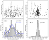 |
Fig. 6. Degree of polarization vs. the polarization position angle of stars projected on BRC 17 (left panel) and BRC 18 (right panel). The histogram of the position angles is also shown. These values are obtained after subtracting the foreground interstellar component from the observed values. The solid black curves represent a fit to the histogram of the position angles using a single Gaussian model. BRC 17 is also fit with a multiple Gaussian model (solid blue), where decomposed Gaussians are shown in dashed blue, and the mean and standard deviation of the central Gaussian are marked. |
3.5. Magnetic field strength using a structure function analysis
After determining the direction of the magnetic field, we estimated the magnetic field strength using the improved Davis–Chandrasekhar–Fermi method (DCF; Davis & Greenstein 1951; Chandrasekhar & Fermi 1953) by determining the turbulent angular dispersion (Hildebrand et al. 2009; Houde et al. 2009). In this method, the dispersion of the polarization angles as a function of distance or angular dispersion function (ADF) is estimated by considering that the net magnetic field consists of a large-scale structured field, B0(x), and a turbulent component, Bt(x). ADF or the square root of the structure-function (SF) is defined as the root mean squared differences between the polarization angles measured for two points separated by a distance l and measured as shown in Eq. (2). Hence, the SF analysis can be used as an important statistical tool to correlate the large-scale structured field and the turbulent component of the magnetic field in molecular clouds (e.g., Hildebrand et al. 2009; Franco et al. 2010; Santos et al. 2012; Eswaraiah et al. 2013; Neha et al. 2016),
![Mathematical equation: $$ \begin{aligned} \langle \Delta \phi ^{2}(l)\rangle ^{1/2} = \Bigg \{\frac{1}{N(l)} \sum \limits _{i = 1}^{N(l)}[\phi (x) - \phi (x+l)]^{2}\Bigg \}^{1/2}. \end{aligned} $$](/articles/aa/full_html/2024/09/aa49720-24/aa49720-24-eq2.gif) (2)
(2)
The structure function within the range δ < l ≪ d (where δ and d are the correlation lengths that characterize Bt(x) and B0(x), respectively) can be estimated using Eq. (3),
 (3)
(3)
where ⟨Δϕ2(l)⟩tot shows the total measured dispersion estimated from the data.  are the measurement uncertainties and are calculated by taking the mean of the variances on Δϕ(l) in each bin. The quantity b2 is the constant turbulent contribution, estimated by the intercept of the fit to the data after subtracting
  . The term m2l2 is a smoothly increasing contribution with the length l (m shows the slope of this linear behavior). All these quantities are statistically independent from each other.
The ratio of the turbulent component and the large-scale magnetic fields is calculated with Eq. (4),
 (4)
(4)
For the BRC 18 region, we estimated the ADF and plotted it with the distance in Fig. 7. We used the polarization angle of 171 stars for BRC 18 to calculate ADF. The measured errors in each bin are very small and are also overplotted in Fig. 7. Each bin denotes  , which is the ADF corrected for the measurement uncertainties. The bin widths are taken on a logarithmic scale. We used only five points, corresponding to a distance smaller than 1 pc, of the ADF in the linear fit of Eq. (3) shown by the dashed line. The shortest distance we considered is ≃0.15 pc. The net turbulent contribution to the angular dispersion, b, was calculated to be 8.9° ± 0.3° (0.15 ± 0.005 rad) for BRC 18. Then, we estimated the ratio of the turbulent component and the large-scale magnetic fields using Eq. (4), which is found to be 0.08 ± 0.004 for BRC 18. The result shows that the turbulent component of the magnetic field is very small compared to the large-scale structured magnetic field, that is, Bt ≪ B0.
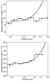 |
Fig. 7. Angular dispersion function (ADF) of the polarization angles, ⟨Δϕ2(l)⟩1/2 (°), with distance (pc) for BRC 18 (upper panel) and BRC 17 (lower panel). The dashed line denotes the best fit to the data up to a distance of 1 pc. |
The strength of the plane-of-the-sky component of the magnetic field was estimated from the modified CF relation (Franco & Alves 2015), as shown in Eq. (5),
![Mathematical equation: $$ \begin{aligned} B_{\rm pos} = 9.3 \left[\frac{2\,n(\mathrm{H}_{2})}{\mathrm{cm}^{-3}}\right]^{1/2} \left[\frac{\Delta V}{\mathrm{km\,s^{-1}}}\right] \left[\frac{b}{1^{\circ }}\right]^{-1}\;\upmu \mathrm{G}. \end{aligned} $$](/articles/aa/full_html/2024/09/aa49720-24/aa49720-24-eq8.gif) (5)
(5)
In Eq. (5), n(H2) is the volume hydrogen density of molecular hydrogen. It was obtained by estimating the hydrogen column density of the region probed by our optical polarimetry and from the radius of the cloud, assuming it to be a spherical cloud. We used the relation N(H2)/AV = 9.4 × 1020 cm−2 mag−1 (Bohlin et al. 1978) to estimate the column density. Based on the method described by Maheswar et al. (2010) and Neha et al. (2016), the average extinction value traced by the stars behind the cloud (assuming a distance ≳400 pc for BRC 18) observed in this study is found to be ∼0.6 mag for BRC 18. We also determined the visual extinction AV using the near-infrared color excess revised (NICER) extinction maps, which are based on 2MASS data (Juvela & Montillaud 2016). The value of AV is found to be 1.6 mag for BRC 18. This is because the method is only sensitive to the extinction of stars that lie in the periphery of the cloud. Hence, we used the average value of AV, which is found to be 1.1 mag. We estimated the radius of BRC 18 by fitting a circle on the WISE 12 μm image. The radius of BRC 18 is determined as ∼1.5 pc, and the volume density is therefore found to be ∼230 cm−3 for BRC 18. We adopted the 12CO line width, ΔV = 1.7 km s−1 for BRC 18, from our molecular line observations (Neha et al., in preparation). After substituting all the values in Eq. (5), the value of Bpos is found to be ∼40 μG for BRC 18. This means that the BRC 18 cloud has a magnetic field strength of ∼40 μG, which is comparable to the moderate magnetic field strength of the simulations, in an almost perpendicular direction to the ionizing radiation. By comparing this with the simulations, we found that the photoionization shock can pass through the cloud without any hindrance and can trigger star formation (Arthur et al. 2011).
The polarization position angles for BRC 17, as shown in Fig. 6, exhibit multiple Gaussian features. We used 71 out of 105 sources whose polarization angles follow the central component in the multi-Gaussian model to estimate the magnetic field strength because it shows a relatively smaller dispersion than the whole data and follows the direction of the ambient magnetic field. We performed a structure-function analysis as described above. The lower panel of Fig. 7 shows a plot of the ADF as a function of distance for BRC 17. Similar to BRC 18, we used five points of the ADF and performed a linear fit using Eq. (4). The value of b is 26.9° ±0.3° for BRC 17. The ratio of the turbulent to the large-scale component of the magnetic field is found to be 0.35 ± 0.22, suggesting that the turbulent component is smaller than the large-scale structured magnetic field. We then estimated the strength of the plane-of-the-sky component of the magnetic field using Eq. (5), adopting n(H2) = 2000 cm−3 and ΔV = 1.3 km s−1 from Zhou et al. (1988), who performed a molecular line observation of BRC 17. The magnetic field is ∼28 μG, which can be considered a weak magnetic field strength. The calculated value of Bpos should be considered a rough estimate due to the large uncertainties of the individual quantities involved in its calculation, particularly for BRC 17, which has a higher b value.
4. Discussion
Based on the radiation-magnetohydrodynamics (R-MHD) simulations of HII regions, Arthur et al. (2011) presented the large-scale magnetic field maps projected on the whole HII region, and they showed that the magnetic field lines are mainly oriented along the large-scale ionization fronts that form a ring around the HII region. The expanding HII and photodissociation regions (PDR) remove the preexisting small-scale disordered magnetic field pattern and produce a large-scale ordered magnetic field in the neutral shell, with an orientation that is approximately parallel to the ionization front. They also reported that the magnetic field lines are aligned in a perpendicular direction to the ionization front at the head of the globules associated with the HII region. Furthermore, Henney et al. (2009) and Mackey & Lim (2011) included the effect of magnetic field on the globules in the presence of ionizing radiation from the OB star. Mackey & Lim (2011) performed 3D radiation magnetohydrodynamics (3D-RMHD) simulations considering three strengths of magnetic fields, 18 μG (weak), 53 μG (medium), and 160 μG (strong) for the direction perpendicular to the ionizing radiation. They found that the RDI process significantly changes the initially weak perpendicular field orientation. The weak field is aligned along the incoming ionizing radiation due to the RDI process and rocket effect. In the medium perpendicular case, slight changes were noted in the field direction, whereas the strong perpendicular magnetic field remained unchanged. Hence, the strong magnetic field can alter the morphology of the structure that developed due to the RDI and rocket effect, in part due to shielding by the dense ionized ridge and in part due to the effect of the magnetic field within the globule.
The direction of the polarization vectors represents the global plane-of-sky magnetic field geometry in LOSFR, which seems to follow the large-scale structure seen in all the images of Fig. 3, which is consistent with the simulations shown by Arthur et al. (2011). Although our sample is small, the polarization vectors clearly follow the ring of the LOSFR in Fig. 3. Fig. 8 shows the global Galactic magnetic field geometry in LOSFR in the optical and submillimeter wavelengths. The Planck image1, taken by the ESA Planck satellite (Planck Collaboration I 2016), shows the submillimeter polarization map and indicates the global magnetic field morphology. In contrast, the black R-band polarization vectors corresponding to the optical magnetic field geometry are overplotted. In the upper part of the image, the magnetic field geometry seems to be organized and regular, which could be due to the large-scale orientation of the magnetic field lines along the Galactic plane. Our optical polarization data are consistent with the submillimeter data, and the orientation of the magnetic field follows the same pattern. It is also seen locally around BRC 17 and BRC 18, as shown in Fig. 9, where the Planck submillimeter polarization vectors along with optical polarization vectors toward BRC 17 and BRC 18 are overplotted on the WISE 12 μm image. These Planck polarization vectors were extracted using Planck public data release 3 (Planck Collaboration I 2016). Since the polarization techniques for both optical and submillimeter wavelengths are different, it would be interesting to compare the two wavelengths because the polarization occurs in the optical due to partial extinction, but in the submillimeter wavelengths, the polarization occurs due to emission.
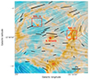 |
Fig. 8. Global magnetic field morphology in LOSFR. The layered texture in the image represents the magnetic field geometry using submillimeter polarization, and the black vectors overplotted on the Planck submillimeter polarization map correspond to the optical magnetic field geometry using the observed R-band polarization. The red star shows the position of λ-Ori. The clouds BRC 17 and BRC 18 are identified. A 2% degree of polarization reference vector is shown for the optical polarization. The image was taken by the ESA Planck satellite (image credit: ESA and the Planck Collaboration). |
The polarization observations of BRC 17 show a wide range of polarization angles with a central peak at 167° and two additional components far away. This could be due to the combined effects of a shock wave from central ionizing source λ-Ori and the HH objects in the vicinity. An abrupt change in the direction of the magnetic field around BRC 17 is noted that is consistent with the Planck observations, as shown in Fig. 9. We binned the polarization vectors along the Galactic longitude for a clear view. Although we lack observations below a Galactic longitude of 192.5°, our polarization vectors show a similar direction as those of Plank, being consistent above longitude > 192.5° and turning toward the high-density material following the Planck vectors. This magnetic field orientation could be the reason for the accumulation of high column densities there, as clouds generally tend to form at kinks or bends in the magnetic field (Passot et al. 1995; Hartmann et al. 2001; Heitsch et al. 2001; Ostriker et al. 2001).
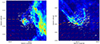 |
Fig. 9. Polarization vectors overplotted on the WISE 12 μm image of BRC 17 (left panel) and BRC 18 (right panel) of our optical data (white) and of the Planck data (red). The binned polarization vectors along Galactic longitude bins are shown in both panels for our data (thick white) and Planck (thick red). The length of the vectors corresponds to the degree of polarization, and the orientation corresponds to the position angle measured from the north and increasing toward the east. The vectors corresponding to a polarization of 2% are shown for reference in their respective colors. |
Magakian et al. (2004) searched HH-objects and emission line stars in star-forming regions and observed an intense molecular outflow spread over ∼5 pc. This is one of the highest-velocity and largest giant outflows known to date. This outflow is known as RNO 43 and is associated with the source (HH 243) IRAS 05295+1247 (Bence et al. 1996). Its outflow velocity is about 11 km s−1 (Wu et al. 2004). A few more HH objects are present in the BRC 17 region. In the head part of BRC 17, HH 176 is present, which is powered by the peculiar A4-type variable star HK-Ori (Lang et al. 2000). This strong high-velocity outflow and the HH objects in the BRC 17 region suggest that star formation activities are ongoing and cloud material is dynamically more active. Zhou et al. (1988) performed molecular line observations toward BRC 17 and showed gas temperature and column density enhancements along the edge of the cloud, which corresponds to the optical bright rim. They also suggested that the gas-heating mechanism in BRC 17 is most likely due to the photoelectric ejection of energetic electrons from dust grains induced by the far-ultraviolet radiation from the λ-Orionis OB association. However, the resolution of these observations is very poor. Further high-resolution molecular line observations can provide a better picture of the kinematics of BRC 17. We calculated the magnetic field strength for BRC 17. The strength of the turbulent component is about 30% of the large-scale magnetic field. The strength of the plane-of-sky component of the magnetic field is ∼28 μG, which can be considered to be in the weak-field regime. It is, therefore, possible that the high-energy radiation affects the orientation of the magnetic field in BRC 17 (Henney et al. 2009; Mackey & Lim 2011). A detailed high-resolution polarimetric study is required to better understand the magnetic field geometry in BRC 17.
BRC 18 shows that the magnetic field lines are aligned in a preferred direction that is roughly perpendicular to the ionizing radiation, which is also consistent with the simulations (Arthur et al. 2011). The directions of the optical polarization vectors are also consistent with Planck, as shown in Fig. 9, where the binned polarization vectors along the Galactic longitude are also plotted, similar to BRC 17. One HH object, HH 175, is also present in BRC 18. Its driving source is IRAS 05417+0907, a multiple system with six components at least (Reipurth & Friberg 2021). Moreover, millimeter observations suggest that the BRC 18 cloud is found to have multiple cores, and the embedded source could be the result of compression by an ionization front driven by the central λ-Ori OB stars (Reipurth & Friberg 2021). We estimated the magnetic field strength for BRC 18 (see Section 3.5) and found ∼40 μG, a medium-strength magnetic field roughly perpendicular to the incoming ionization radiations. The moderate magnetic field strength does not strongly affect the interaction of the ionization radiations with the cloud but tries to align along the incoming ionizing radiations (Arthur et al. 2011). Some of the polarization vectors in the lower region of BRC 18 (see the right panel of Fig. 5) show that they align themselves along the incoming ionizing radiation, suggesting RDI in BRC 18.
5. Conclusions
We presented optical polarimetric results for the stars that are globally projected on the LOSFR and the associated BRC 17 and BRC 18. Using these polarimetric observations, we studied the importance of the magnetic field in the evolution of the HII region. We list our conclusions below.
-
We estimated the distance of LOSFR as 392 ± 8 pc using astrometry information of YSOs toward BRC 17, BRC 18, and members of the central cluster Collinder 69 using Gaia EDR3.
-
We found a large-scale ordered magnetic field in the LOSFR, and our results are consistent with the simulations and the Planck submillimeter polarization map. The orientation of the magnetic field is almost similar in all three optical bands, VRI and submillimeter.
-
The magnetic field lines traced by the polarization position angles in BRC 17 are roughly oriented in the north-south direction but show a large dispersion. In the case of BRC 18, the magnetic field morphology is regular. The orientation is approximately perpendicular to the incoming ionizing radiation. The magnetic field geometry in these two regions is also consistent with the Planck magnetic field map.
-
The average dust size in the LOSFR was also determined using Serkowski’s curve fitting, which is ∼0.51 ± 0.05 μm, and the average value of the total-to-selective extinction ratio RV is equal to ∼2.9 ± 0.3, which is consistent with the general value of the ISM for the Milky Way.
-
The ratio of the turbulent to large-scale magnetic field strength was estimated to be higher than ∼30% in BRC 17 compared to 10% in BRC 18. The plane-of-the-sky magnetic field strength, calculated using the structure function analysis, is ∼28 μG for BRC 17 and ∼40 μG for BRC 18.
Acknowledgments
We thank the referee for her/his constructive suggestions/comments, which helped us to improve the quality of our manuscript. This research has made use of the SIMBAD database, operated at CDS, Strasbourg, France. We also acknowledge the use of NASA’s SkyView facility (http://skyview.gsfc.nasa.gov) located at NASA Goddard Space Flight Center. NS acknowledges the financial support provided under the National Post-doctoral Fellowship (NPDF; File Number: PDF/2022/001040) by the Science & Engineering Research Board (SERB), a statutory body of the Department of Science & Technology (DST), Government of India. NS thanks Suvendu Rakshit for the useful discussions.
References
- Arthur, S. J., Henney, W. J., Mellema, G., de Colle, F., & Vázquez-Semadeni, E. 2011, MNRAS, 414, 1747 [Google Scholar]
- Bailer-Jones, C. A. L., Rybizki, J., Fouesneau, M., Demleitner, M., & Andrae, R. 2021, AJ, 161, 147 [Google Scholar]
- Ballesteros-Paredes, J., Hartmann, L., & Vázquez-Semadeni, E. 1999, ApJ, 527, 285 [NASA ADS] [CrossRef] [Google Scholar]
- Barnard, E. E. 1919, ApJ, 49, 1 [NASA ADS] [CrossRef] [Google Scholar]
- Bayo, A., Barrado, D., Huélamo, N., et al. 2012, A&A, 547, A80 [NASA ADS] [CrossRef] [EDP Sciences] [Google Scholar]
- Bence, S. J., Richer, J. S., & Padman, R. 1996, MNRAS, 279, 866 [Google Scholar]
- Bertoldi, F. 1989, ApJ, 346, 735 [Google Scholar]
- Bohlin, R. C., Savage, B. D., & Drake, J. F. 1978, ApJ, 224, 132 [Google Scholar]
- Chandrasekhar, S., & Fermi, E. 1953, ApJ, 118, 113 [Google Scholar]
- Chauhan, N., Pandey, A. K., Ogura, K., et al. 2009, MNRAS, 396, 964 [NASA ADS] [CrossRef] [Google Scholar]
- Cortés, P. C., Sanhueza, P., Houde, M., et al. 2021, ApJ, 923, 204 [CrossRef] [Google Scholar]
- Cutri, R. M., Skrutskie, M. F., van Dyk, S., et al. 2003, VizieR Online Data Catalog: II/246 [Google Scholar]
- Davis, L., & Greenstein, J. L. 1951, ApJ, 114, 206 [NASA ADS] [CrossRef] [Google Scholar]
- Dolan, C. J., & Mathieu, R. D. 1999, AJ, 118, 2409 [Google Scholar]
- Dolan, C. J., & Mathieu, R. D. 2001, AJ, 121, 2124 [NASA ADS] [CrossRef] [Google Scholar]
- Dolan, C. J., & Mathieu, R. D. 2002, AJ, 123, 387 [Google Scholar]
- Duerr, R., Imhoff, C. L., & Lada, C. J. 1982, ApJ, 261, 135 [NASA ADS] [CrossRef] [Google Scholar]
- Elmegreen, B. G. 2011, in EAS Publications Series, eds. C. Charbonnel, & T. Montmerle, 51, 45 [NASA ADS] [CrossRef] [EDP Sciences] [Google Scholar]
- Eswaraiah, C., Pandey, A. K., Maheswar, G., et al. 2011, MNRAS, 411, 1418 [NASA ADS] [CrossRef] [Google Scholar]
- Eswaraiah, C., Pandey, A. K., Maheswar, G., et al. 2012, MNRAS, 419, 2587 [NASA ADS] [CrossRef] [Google Scholar]
- Eswaraiah, C., Maheswar, G., Pandey, A. K., et al. 2013, A&A, 556, A65 [NASA ADS] [CrossRef] [EDP Sciences] [Google Scholar]
- Franco, G. A. P., & Alves, F. O. 2015, ApJ, 807, 5 [Google Scholar]
- Franco, G. A. P., Alves, F. O., & Girart, J. M. 2010, ApJ, 723, 146 [Google Scholar]
- Gaia Collaboration (Brown, A. G. A., et al.) 2021, A&A, 649, A1 [NASA ADS] [CrossRef] [EDP Sciences] [Google Scholar]
- Garcia-Segura, G., & Franco, J. 1996, ApJ, 469, 171 [NASA ADS] [CrossRef] [Google Scholar]
- Hartmann, L., Ballesteros-Paredes, J., & Bergin, E. A. 2001, ApJ, 562, 852 [NASA ADS] [CrossRef] [Google Scholar]
- Hayashi, M., Itoh, Y., & Oasa, Y. 2012, PASJ, 64, 96 [NASA ADS] [CrossRef] [Google Scholar]
- Heiles, C. 2000, AJ, 119, 923 [Google Scholar]
- Heitsch, F., Mac Low, M.-M., & Klessen, R. S. 2001, ApJ, 547, 280 [NASA ADS] [CrossRef] [Google Scholar]
- Henney, W. J., Arthur, S. J., de Colle, F., & Mellema, G. 2009, MNRAS, 398, 157 [NASA ADS] [CrossRef] [Google Scholar]
- Hildebrand, R. H., Kirby, L., Dotson, J. L., Houde, M., & Vaillancourt, J. E. 2009, ApJ, 696, 567 [Google Scholar]
- Høg, E., Fabricius, C., Makarov, V. V., et al. 2000, A&A, 355, L27 [Google Scholar]
- Hosoya, K., Itoh, Y., Oasa, Y., Gupta, R., & Sen, A. K. 2019, Int. J. Astron. Astrophys., 9, 154 [NASA ADS] [CrossRef] [Google Scholar]
- Houde, M., Vaillancourt, J. E., Hildebrand, R. H., Chitsazzadeh, S., & Kirby, L. 2009, ApJ, 706, 1504 [Google Scholar]
- Juvela, M., & Montillaud, J. 2016, A&A, 585, A38 [NASA ADS] [CrossRef] [EDP Sciences] [Google Scholar]
- Koenig, X., Hillenbrand, L. A., Padgett, D. L., & DeFelippis, D. 2015, AJ, 150, 100 [NASA ADS] [CrossRef] [Google Scholar]
- Kounkel, M., Covey, K., Suárez, G., et al. 2018, AJ, 156, 84 [NASA ADS] [CrossRef] [Google Scholar]
- Lang, W. J., Masheder, M. R. W., Dame, T. M., & Thaddeus, P. 2000, A&A, 357, 1001 [NASA ADS] [Google Scholar]
- Lindegren, L. 2018, Re-normalising the Astrometric Chi-square in Gaia DR2 (Lund Observatory) [Google Scholar]
- Lindegren, L., Klioner, S. A., Hernández, J., et al. 2021, A&A, 649, A2 [EDP Sciences] [Google Scholar]
- Liu, J., Qiu, K., Berry, D., et al. 2019, ApJ, 877, 43 [NASA ADS] [CrossRef] [Google Scholar]
- Mackey, J., & Lim, A. J. 2010, MNRAS, 403, 714 [NASA ADS] [CrossRef] [Google Scholar]
- Mackey, J., & Lim, A. J. 2011, MNRAS, 412, 2079 [NASA ADS] [CrossRef] [Google Scholar]
- Magakian, T. Y., Movsessian, T. A., & Nikogossian, E. H. 2004, Astrophysics, 47, 162 [NASA ADS] [CrossRef] [Google Scholar]
- Maheswar, G., Lee, C. W., Bhatt, H. C., Mallik, S. V., & Dib, S. 2010, A&A, 509, A44 [NASA ADS] [CrossRef] [EDP Sciences] [Google Scholar]
- Mathieu, R. D. 2008, in Handbook of Star Forming Regions, ed. B. Reipurth, 757 [Google Scholar]
- McKee, C. F., & Ostriker, E. C. 2007, ARA&A, 45, 565 [Google Scholar]
- Miao, J., White, G. J., Nelson, R., Thompson, M., & Morgan, L. 2006, MNRAS, 369, 143 [NASA ADS] [CrossRef] [Google Scholar]
- Mouschovias, T. C. 1978, in IAU Colloq. 52: Protostars and Planets, ed. T. Gehrels, 209 [Google Scholar]
- Murdin, P., & Penston, M. V. 1977, MNRAS, 181, 657 [Google Scholar]
- Neha, S., Maheswar, G., Soam, A., Lee, C. W., & Tej, A. 2016, A&A, 588, A45 [NASA ADS] [CrossRef] [EDP Sciences] [Google Scholar]
- Neha, S., Maheswar, G., Soam, A., & Lee, C. W. 2018, MNRAS, 476, 4442 [NASA ADS] [CrossRef] [Google Scholar]
- Orsatti, A. M., Vega, E., & Marraco, H. G. 1998, AJ, 116, 266 [NASA ADS] [CrossRef] [Google Scholar]
- Orsatti, A. M., Feinstein, C., Vergne, M. M., Martínez, R. E., & Vega, E. I. 2010, A&A, 513, A75 [NASA ADS] [CrossRef] [EDP Sciences] [Google Scholar]
- Ostriker, E. C., Stone, J. M., & Gammie, C. F. 2001, ApJ, 546, 980 [Google Scholar]
- Passot, T., Vazquez-Semadeni, E., & Pouquet, A. 1995, ApJ, 455, 536 [NASA ADS] [CrossRef] [Google Scholar]
- Pattle, K., Lai, S.-P., Francesco, J. D., et al. 2021, ApJ, 907, 88 [NASA ADS] [CrossRef] [Google Scholar]
- Perryman, M. A. C., Lindegren, L., Kovalevsky, J., et al. 1997, A&A, 323, L49 [Google Scholar]
- Planck Collaboration I. 2016, A&A, 594, A1 [NASA ADS] [CrossRef] [EDP Sciences] [Google Scholar]
- Ramaprakash, A. N., Gupta, R., Sen, A. K., & Tandon, S. N. 1998, A&AS, 128, 369 [NASA ADS] [CrossRef] [EDP Sciences] [Google Scholar]
- Rautela, B. S., Joshi, G. C., & Pandey, J. C. 2004, Bull. Astron. Soc. India, 32, 159 [NASA ADS] [Google Scholar]
- Reipurth, B. 2000, VizieR Online Data Catalog: V/104 [Google Scholar]
- Reipurth, B., & Friberg, P. 2021, MNRAS, 501, 5938 [Google Scholar]
- Saha, P., Gopinathan, M., Ojha, D. K., & Neha, S. 2022, MNRAS, 510, 2644 [NASA ADS] [CrossRef] [Google Scholar]
- Santos, F. P., Roman-Lopes, A., & Franco, G. A. P. 2012, ApJ, 751, 138 [NASA ADS] [CrossRef] [Google Scholar]
- Schmidt, G. D., Elston, R., & Lupie, O. L. 1992, AJ, 104, 1563 [Google Scholar]
- Serkowski, K., Mathewson, D. S., & Ford, V. L. 1975, ApJ, 196, 261 [NASA ADS] [CrossRef] [Google Scholar]
- Sharpless, S. 1959, ApJS, 4, 257 [Google Scholar]
- Soam, A., Maheswar, G., Bhatt, H. C., Lee, C. W., & Ramaprakash, A. N. 2013, MNRAS, 432, 1502 [NASA ADS] [CrossRef] [Google Scholar]
- Soam, A., Maheswar, G., Lee, C. W., et al. 2015, A&A, 573, A34 [NASA ADS] [CrossRef] [EDP Sciences] [Google Scholar]
- Soam, A., Maheswar, G., Lee, C. W., Neha, S., & Andersson, B. G. 2017, MNRAS, 465, 559 [Google Scholar]
- Soam, A., Maheswar, G., Lee, C. W., Neha, S., & Kim, K.-T. 2018, MNRAS, 476, 4782 [Google Scholar]
- Soler, J. D., Hennebelle, P., Martin, P. G., et al. 2013, ApJ, 774, 128 [Google Scholar]
- Sugitani, K., Fukui, Y., & Ogura, K. 1991, ApJS, 77, 59 [NASA ADS] [CrossRef] [Google Scholar]
- Topasna, G. A., Daman, E. A., & Kaltcheva, N. T. 2017, PASP, 129, 104201 [NASA ADS] [CrossRef] [Google Scholar]
- van Leeuwen, F. 2007, A&A, 474, 653 [CrossRef] [EDP Sciences] [Google Scholar]
- Vergne, M. M., Feinstein, C., & Martínez, R. 2007, A&A, 462, 621 [NASA ADS] [CrossRef] [EDP Sciences] [Google Scholar]
- Wade, C. M. 1957, AJ, 62, 148 [Google Scholar]
- Whittet, D. C. B. 1977, MNRAS, 180, 29 [NASA ADS] [Google Scholar]
- Whittet, D. C. B., & van Breda, I. G. 1978, A&A, 66, 57 [NASA ADS] [Google Scholar]
- Wu, Y., Wei, Y., Zhao, M., et al. 2004, A&A, 426, 503 [NASA ADS] [CrossRef] [EDP Sciences] [Google Scholar]
- Zamora-Avilés, M., Vázquez-Semadeni, E., González, R. F., et al. 2019, MNRAS, 487, 2200 [CrossRef] [Google Scholar]
- Zari, E., Hashemi, H., Brown, A. G. A., Jardine, K., & de Zeeuw, P. T. 2018, A&A, 620, A172 [NASA ADS] [CrossRef] [EDP Sciences] [Google Scholar]
- Zhang, C. Y., Laureijs, R. J., Chlewicki, G., Wesselius, P. R., & Clark, F. O. 1989, A&A, 218, 231 [NASA ADS] [Google Scholar]
- Zhou, S., Butner, H. M., & Evans, N. J. 1988, ApJ, 333, 809 [NASA ADS] [CrossRef] [Google Scholar]
Appendix A: Additional table
Polarization results for the observed Tycho stars in the VRI filters toward the λ-Ori region.
Polarization results of 105 stars observed in the direction of BRC 17 and 171 stars observed toward BRC 18 with P/σP ≥ 2 in the R filter.
All Tables
Polarization values of the observed foreground stars and from the Heiles catalog.
Mean values of λmax and Pmax for the UBVRI, BVRI, and VRI dataset for various regions.
Polarization results for the observed Tycho stars in the VRI filters toward the λ-Ori region.
Polarization results of 105 stars observed in the direction of BRC 17 and 171 stars observed toward BRC 18 with P/σP ≥ 2 in the R filter.
All Figures
|
Fig. 1. Proper motion values of the known candidate YSOs associated with BRC 17 (left panel) and the known probable cluster members associated with Collinder 69 (right panel) plotted as a function of their distances obtained from Gaia EDR3. Panels a and c: μα vs. d plot of the sources. The candidate YSOs and cluster members lying within a 5 × MAD boundary in the μα vs. d plot are plotted using filled blue circles, and the outliers are plotted using open gray circles. The dashed lines indicate the median values of μα and d of the candidate YSOs and cluster members. Panels b and d: μδ vs. d plot of the sources. The gray shaded ellipses show the 5 × MAD boundary range in distance and proper motions within which the sources are used to estimate a distance. The candidate YSOs and cluster members lying within the 5 × MAD boundary in the μδ vs. d plot are plotted using filled blue circles, and the outliers are plotted using open gray circles. The dashed lines indicate the median values of d and μδ of the candidate YSOs and cluster members. |
| In the text | |
|
Fig. 2. Polarization angle vs. distance of the foreground stars found within a diameter of 1° around BRC 17, BRC 18, and the Heiles stars found within a diameter of 9° around λ-Ori (upper panel). Degree of polarization vs. distance for the same stars (lower panel). The dashed gray line corresponds to a distance of 392 pc in both panels. The distances are calculated from the HIPPARCOS parallax measurements taken from van Leeuwen (2007) and adopted from Bailer-Jones et al. (2021). The gray circles show the bright Tycho stars behind the cloud. The distances for the Tycho stars are taken from Bailer-Jones et al. (2021). |
| In the text | |
|
Fig. 3. Polarization vectors of 34 bright Tycho stars plotted in the Planck 857 GHz image of LOSFR in the V band (upper panel), R band (middle panel), and I band (lower panel). The length of the vectors corresponds to the degree of the polarization values, while the orientation represents the polarization angle measured from north to east. A vector with a polarization of 2% is shown for reference. The dashed white line shows the position of the Galactic plane. The white star shows the position of λ-Ori. |
| In the text | |
|
Fig. 4. Serkowski curve for 34 bright Tycho stars observed in the VRI filters. The filled blue, green, and red circles correspond to the V, R, and I bands, respectively. The solid magenta line represents the fitting using the Serkowski law (Serkowski et al. 1975). |
| In the text | |
|
Fig. 5. Polarization vectors overplotted on the WISE 12 μm image of BRC 17 (left panel) and BRC 18 (right panel). The length of the vectors corresponds to the degree of polarization, and the orientation corresponds to the position angle measured from the north and increasing toward the east. A vector corresponding to a polarization of 2% is shown for reference. The dashed white line shows the orientation of the Galactic plane. The red star shows the location of IRAS sources, and the yellow stars show the positions of HH objects in both images (Reipurth 2000). The green arrows in both panels show the outflow directions. The outflow sources are HH 243 for BRC 17 and IRAS 05417+0907 for BRC 18. |
| In the text | |
|
Fig. 6. Degree of polarization vs. the polarization position angle of stars projected on BRC 17 (left panel) and BRC 18 (right panel). The histogram of the position angles is also shown. These values are obtained after subtracting the foreground interstellar component from the observed values. The solid black curves represent a fit to the histogram of the position angles using a single Gaussian model. BRC 17 is also fit with a multiple Gaussian model (solid blue), where decomposed Gaussians are shown in dashed blue, and the mean and standard deviation of the central Gaussian are marked. |
| In the text | |
|
Fig. 7. Angular dispersion function (ADF) of the polarization angles, ⟨Δϕ2(l)⟩1/2 (°), with distance (pc) for BRC 18 (upper panel) and BRC 17 (lower panel). The dashed line denotes the best fit to the data up to a distance of 1 pc. |
| In the text | |
|
Fig. 8. Global magnetic field morphology in LOSFR. The layered texture in the image represents the magnetic field geometry using submillimeter polarization, and the black vectors overplotted on the Planck submillimeter polarization map correspond to the optical magnetic field geometry using the observed R-band polarization. The red star shows the position of λ-Ori. The clouds BRC 17 and BRC 18 are identified. A 2% degree of polarization reference vector is shown for the optical polarization. The image was taken by the ESA Planck satellite (image credit: ESA and the Planck Collaboration). |
| In the text | |
|
Fig. 9. Polarization vectors overplotted on the WISE 12 μm image of BRC 17 (left panel) and BRC 18 (right panel) of our optical data (white) and of the Planck data (red). The binned polarization vectors along Galactic longitude bins are shown in both panels for our data (thick white) and Planck (thick red). The length of the vectors corresponds to the degree of polarization, and the orientation corresponds to the position angle measured from the north and increasing toward the east. The vectors corresponding to a polarization of 2% are shown for reference in their respective colors. |
| In the text | |
Current usage metrics show cumulative count of Article Views (full-text article views including HTML views, PDF and ePub downloads, according to the available data) and Abstracts Views on Vision4Press platform.
Data correspond to usage on the plateform after 2015. The current usage metrics is available 48-96 hours after online publication and is updated daily on week days.
Initial download of the metrics may take a while.