| Issue |
A&A
Volume 689, September 2024
|
|
|---|---|---|
| Article Number | A279 | |
| Number of page(s) | 14 | |
| Section | Numerical methods and codes | |
| DOI | https://doi.org/10.1051/0004-6361/202449700 | |
| Published online | 19 September 2024 | |
An effective model for the tidal disruption of satellites undergoing minor mergers with axisymmetric primaries
1
Università degli Studi di Milano-Bicocca,
Piazza della Scienza 3,
20126
Milano,
Italy
2
INFN, Sezione di Milano-Bicocca,
Piazza della Scienza 3,
20126
Milano,
Italy
3
INAF – Osservatorio Astronomico di Brera,
via Brera 20,
20121
Milano,
Italy
4
DiSAT, Università degli Studi dell’Insubria,
via Valleggio 11,
22100
Como,
Italy
Received:
22
February
2024
Accepted:
25
June
2024
Abstract
According to the hierarchical formation paradigm, galaxies form through mergers of smaller entities and massive black holes (MBHs), if present at their centers, migrate to the nucleus of the newly formed galaxy, where they form binary systems. The formation and evolution of MBH binaries, and in particular their coalescence timescale, is highly relevant for current and future facilities aimed at detecting the gravitational wave signal produced by the MBHs close to coalescence. While most of the studies targeting this process are based on hydrodynamic simulations, the high computational cost makes a complete parameter space exploration prohibitive. Semianalytic approaches represent a valid alternative, but they require ad hoc prescriptions for the mass loss of the merging galaxies in minor mergers due to tidal stripping, which is not commonly considered or is at best modelled assuming very idealised geometries. In this work we propose a novel, effective model for the tidal stripping in axisymmetric potentials, to be implemented in semi-analytic models. We validated our semi-analytic approach against N-body simulations considering different galaxy sizes, inclinations, and eccentricities, finding only a moderate dependence on the orbit eccentricity. In particular, we find that, for almost circular orbits, our model mildly overestimates the mass loss, and this is due to the adjustment of the stellar distribution after the mass is removed. Nonetheless, the model exhibits a very good agreement with simulations in all the considered conditions, and thus represents an extremely powerful addition to semi-analytic calculations.
Key words: methods: analytical / methods: numerical / galaxies: evolution / galaxies: interactions / galaxies: kinematics and dynamics
Corresponding author; This email address is being protected from spambots. You need JavaScript enabled to view it.
© The Authors 2024
 Open Access article, published by EDP Sciences, under the terms of the Creative Commons Attribution License (https://creativecommons.org/licenses/by/4.0), which permits unrestricted use, distribution, and reproduction in any medium, provided the original work is properly cited.
This article is published in open access under the Subscribe to Open model. This email address is being protected from spambots. You need JavaScript enabled to view it. to support open access publication.
1 Introduction
In the framework of the hierarchical paradigm of cosmic structure formation (Press & Schechter 1974; White & Rees 1978), galaxies form in a bottom-up fashion, whereby the massive galaxies that we see today build up at the intersection of dark matter (DM) filaments along which other galaxies and cold gas can stream inwards (Dekel et al. 2009). Specifically, at those ‘cosmic crossroads’, galaxies are expected to experience a sequence of mergers and accretion events that contribute to their final mass and morphological appearance.
Galactic mergers are categorised based on the mass ratio of the involved galaxy pairs. The threshold between minor and major mergers is not universally determined; different values are employed in the literature depending on the specific research objectives and contexts. Callegari et al. (2011) classify as major mergers systems involving galaxies with a mass ratio exceeding 1:10, while those falling below this value are designated as minor mergers. A widely used classification defines major mergers as systems with a mass ratio grater than 1:3, and minor merger as those falling in the range 1:3–1:10 (e.g. Cox et al. 2008; Hopkins et al. 2009; Moreno et al. 2021; Renaud et al. 2009). Ventou et al. (2019) categorise galaxy pairs on the basis of the stellar mass ratio of the systems involved, defining as major, minor, and very minor mergers the systems corresponding to the ranges 1:1–1:6, 1:6–1:100 and < 1:100, respectively.
Besides the specific choice of the threshold, the distinction between minor and major mergers is not a mere classification, but implies very different dynamical evolutions, outcomes and investigation techniques. Major mergers are generally rare and disruptive events that completely reshuffle the material in the parent systems and significantly perturb the original morphology in a few dynamical times. Given their disruptive effect, they can be properly characterised only through expensive numerical simulations able to track the strongly time-varying gravitational potential. On the contrary, minor mergers are usually common events over galaxy lifetimes and they generally represent a (small to moderate) perturbation to the more massive system into which they sink. In this regard, the secondary galaxies involved in minor galaxy mergers can be treated as massive perturbers, that is, objects considerably heavier than the single bodies forming the galactic structure but much less massive than the whole host galaxy. By leaving the more massive galaxy nearly unchanged, minor mergers can be modelled in a semi-analytical fashion (e.g. Hilz et al. 2012). This feature opens the possibility of performing investigations with inexpensive computational loads, but which still require a proper and careful tuning of the semi-analytical recipes against numerical simulations.
Even though single minor mergers do not typically morphologically transform host galaxies1, recent theoretical and observational studies highlight the important role that repeated minor mergers can play in the evolution of their massive companions. The occurrence of multiple minor mergers in disc galaxies can gradually induce a significant redistribution of the stellar orbits in the primary system, thus forming slowly rotating spheroidal remnants (see e.g. Bournaud et al. 2007; Qu et al. 2011; Taranu et al. 2013). Martin et al. (2018) show that one-third of the morphological transformations of galaxies undergoing galaxy mergers over cosmic time are due to repeated minor merger events, which become the dominant driver of morphological changes at late epochs (z ≳ 1). Moreover, minor mergers have been proven to enhance both star formation (they are responsible for over half of the star formation events induced by galaxy mergers in the Universe) and massive black hole (MBH) accretion rates (Kaviraj 2014; Pace & Salim 2014), and also to be responsible for 70% of the merger-driven asymmetric structures in post-merger galaxy remnants (Bottrell et al. 2024).
Among the massive perturbers inhabiting galaxies, MBHs are particularly interesting to study. MBHs are located in the nuclei of most massive galaxies (if not all of them; see e.g. Ferrarese & Ford 2005; Kormendy & Ho 2013) and through galaxy mergers multiple MBHs are delivered within the same host, eventually leading to the formation of MBH binaries, triplets or even higher-order multiplets (Begelman et al. 1980; Volonteri et al. 2003; Bonetti et al. 2018). These systems are primary targets of current and forthcoming gravitational wave experiments, primarily the Pulsar Timing Array (PTA; Agazie et al. 2023; Antoniadis et al. 2023; Reardon et al. 2023) campaigns now opening up the nanohertz sky, and the Laser Interferometer Space Antenna (LISA), targeting millihertz frequencies (Amaro-Seoane et al. 2017). Prior to the formation of bound MBH systems in the nuclei of galaxies, every MBH needs to sink towards the central regions. The main actor driving this evolution is dynamical friction (DF; Chandrasekhar 1943). At this stage of the evolution MBHs are generally still surrounded by their progenitors’ cores, so their effective sinking mass (which locally perturbs the primary and leads to DF) can be much higher than the mass of the MBH itself (Neumayer et al. 2020). However, such leftover material (gas and stars) surrounding the MBH typically gets gradually stripped by the main galaxy tidal field (Binney & Tremaine 1987). The effectiveness of the process depends on the compactness of the material around the intruder MBH, and on the steepness of the galactic acceleration field. Depending on the efficiency of the stripping process, the MBH loses material and cam eventually ‘get naked’, that is, remain without any residual surrounding distribution of matter bound to it. This effective ‘mass loss’ crucially affects the dynamics of the inspiral and especially the efficiency of DF, as the DF timescale needed for the object to reach the centre of the primary galaxy critically depends on the perturber’s mass (see e.g. Volonteri et al. 2020).
A quantitative assessment of how mass is stripped from infalling satellite galaxies requires a careful estimation of the so-called tidal radius (i.e. the conceptual boundary dividing the bound from the unbound mass of a celestial object). Beyond this limit, the object’s material undergoes stripping due to the tidal field of the more massive companion. First introduced by von Hoerner (1957) within the context of Milky Way globular clusters, the tidal radius is theoretically defined strictly for satellites on circular orbits, where it coincides with the position of the L1 or L2 Lagrange points (Binney & Tremaine 1987). A different attempt to also define such a radius also for eccentric motion was explored by King (1962), who argued that during pericentre passages, satellites are truncated to the size indicated by the pericentric tidal radius. Later, Henon (1970) and Keenan & Innanen (1975) observed that retrograde orbits in the context of the restricted three-body problem are stable over greater distances compared to prograde orbits, farther out than the tidal radius defined by King (1962). In a more recent study, Read et al. (2006) derived an expression for the tidal radius, taking different orbit types into account: prograde, radial, and retrograde. Interestingly, their analysis revealed that the tidal radius for retrograde orbits exceeds that of radial orbits, which, in turn, is larger than the tidal radius for prograde orbits.
To date, the vast majority of attempts to estimate the tidal radius have focused on spherically symmetric host galaxies (see however Gajda & Łokas 2016). Although observations show that while the morphology of massive galaxies in the local Universe is dominated by spheroidal systems (see e.g. Bernardi et al. 2003; Conselice et al. 2014), in the early Universe the massive galaxy population was mostly composed of disc galaxies (see e.g. Buitrago et al. 2014; Shibuya et al. 2015). This morphological transformation which leads to an overall transition from rotationally supported systems to dispersion-dominated ones, is believed to be primarily driven by galaxy mergers. Moreover, cosmological simulations suggest that disc galaxies do not show any significant difference in their merger history compared to spheroidal galaxies (see e.g. Martin et al. 2018). Thus, a significant number of mergers involving disc-like primary galaxies are expected to have occurred throughout cosmic history and are still ongoing. Indeed, observations on nearby massive disc galaxies display tidal features, hinting that they have undergone recent minor merger events. For this reason, a systematic investigation focused on galaxy mergers involving systems that strongly deviate from spherical symmetry is compelling.
In this study, we aim to find a general description of the tidal radius when axis-symmetric systems are involved2. These systems, representative of, for example, spiral galaxies, are quite common and many minor mergers occur in such galaxies. Our ultimate goal consists in deriving a simplified prescription for the tidal radius to be implemented in semi-analytical models of galaxy formation in order to better assess the DF-driven inspiral pace of massive perturbers within galaxies of any type.
A proper and comprehensive semi-analytical modellisation of minor mergers can be a powerful tool for studying a wide variety of astrophysical scenarios. The exploitation of semianalytical models is crucial to overcoming the limited spacial and mass resolution of large-scale cosmological simulations. In these simulations, numerous minor mergers are observed to occur; however, the lack of sufficient resolution may hinder our ability to track the late stages of these events as the satellite galaxies become unresolved. Employing detailed semi-analytical models would enable us to follow the satellite evolution down to scales where the system is no longer resolved in the simulations. This feature allows us to predict the late phases of the merger and to determine the ultimate fate of the satellite galaxy and, if present, of the MBH embedded within it. In this context, semi-analytical models could be useful, for instance, for addressing and possibly reconciling discrepancies between the estimated fraction of orphan galaxies arising from mock and semi-empirical models (see e.g. Kumar et al. 2024). Furthermore, due to their great versatility, semi-analytical models are particularly well suited for studying the formation and evolution of systems in extreme merger scenarios, such as very faint Milky Way satellites (Smith et al. 2024). Finally, minor mergers may also trigger an enhancement in the satellite MBH accretion due to gas inflows caused by shocks developing within the interstellar medium either in the pairing phase at the contact surface of the two galaxies (Capelo & Dotti 2017) or in the final phases when the naked MBH circularises inside the primary disc (Callegari et al. 2011).
This paper is organised as follows: in Sec. 2, we introduce a novel prescription for the tidal radius, delineate the galactic models employed, and detail the setup of the N-body simulations implemented for our prescription validation. In Sec. 3, we present the outcomes of the comparison between our model’s predictions and those derived from N-body simulations. Finally, in Sec. 4 we discuss the limitations of our model, summarise our findings, and draw our conclusions.
2 Methods
When minor mergers occur, satellite galaxies, while orbiting within their hosts, are subjected to tidal forces that remove part of their mass, sometimes leading to their complete disruption even after a single pericentre passage. Two main mechanisms have been identified for removing mass from the satellite, depending on the rapidity at which the external tidal field varies. When the satellite experiences a slowly changing tidal field, the effect of the tidal forces is that of stripping material from the outer regions of the satellite, forming a clear external boundary often called the tidal radius (Rt). This process is identified as ‘tidal stripping’. On the contrary, when the satellite undergoes a rapid change in the external tidal field, part of its orbital energy is converted into internal energy, leading to an overall heating of the satellite. The amount of energy injected into the system during fast pericentre passages and transferred to the stars can be enough to unbind a significant fraction of the satellite mass. This effect is known as ‘tidal heating’. The mass loss caused by tidal effects can significantly impact the orbital decay of the satellite as it reduces the efficiency at which DF drags the satellite galaxy towards the centre of its host, thus increasing its orbital decay time.
2.1 Tidal radius
To characterise the mass loss of satellite galaxies due to tidal stripping in minor mergers, the first step consists of defining the tidal radius. The standard approach in literature considers two spherically symmetric systems, with mass profiles m(r) for the satellite, and M(r) for the host galaxy, whose centres are separated by a distance R. The satellite Rt is defined as the distance from the centre of the satellite at which the acceleration of a test particle along the direction connecting the centre of the two systems vanishes. In a minor merger scenario where m ≪ M, under the assumptions that Rt ≪ R at any time, and that the test particle has null velocity in the satellite’s reference frame, Rt is given by
![Mathematical equation: $\[R_t=R\left[\frac{G m\left(R_t\right)}{\Omega^2-\frac{\mathrm{d}^2 \Phi_h}{\mathrm{~d} r^2}}\right]^{\frac{1}{3}}.\]$](/articles/aa/full_html/2024/09/aa49700-24/aa49700-24-eq1.png) (1)
(1)
This expression was first derived in King (1962), where r and Ω are the radial coordinate and the angular velocity of the satellite in the reference frame of the host galaxy, and Φh(r) is its gravitational potential. It is worth noting that this formula is strictly valid for circular orbits, but can be easily extended to eccentric orbits if one considers instantaneous values for Ω and R. Additionally, it is important to emphasise that Eq. (1) holds only under the simplistic assumption of a spherical host.
In this study, we present a novel prescription for Rt that is adaptable to various host geometries. For this purpose, we considered a spherically symmetric satellite galaxy embedded in the generic potential of its host. We defined the galactic iner-tial frame with the origin in the galactic centre denoted as S and the non-inertial frame of the satellite as S′. In this work, all the quantities evaluated in the non-inertial frame of the satellite are primed, while the unprimed are relative to the inertial frame of the host galaxy. Considering a test satellite star, its position is identified by the radius vector r*. The acceleration of the test star in the reference frame of the satellite is
![Mathematical equation: $\[\mathbf{a}^{\prime}=\mathbf{a}-\mathbf{A}-\frac{\mathrm{d} \boldsymbol{\Omega}}{\mathrm{d} t} \times \mathbf{r}_*^{\prime}-\boldsymbol{\Omega} \times\left(\boldsymbol{\Omega} \times \mathbf{r}_*^{\prime}\right)-2 \boldsymbol{\Omega} \times \mathbf{v}^{\prime}.\]$](/articles/aa/full_html/2024/09/aa49700-24/aa49700-24-eq2.png) (2)
(2)
Here, Ω is the angular velocity of the satellite centre of mass (CoM), a represents the acceleration of the test star in the S frame
![Mathematical equation: $\[\mathbf{a}=-\frac{G M_s\left(r_*^{\prime}\right)}{r_*^{\prime 3}} \mathbf{r}_*^{\prime}-\nabla \phi_h\left(r_*\right),\]$](/articles/aa/full_html/2024/09/aa49700-24/aa49700-24-eq3.png) (3)
(3)
and A is the acceleration of the S′ frame in S, which can be expressed as
![Mathematical equation: $\[\mathbf{A}=-\nabla \phi_h\left(r_S\right),\]$](/articles/aa/full_html/2024/09/aa49700-24/aa49700-24-eq4.png) (4)
(4)
where rS indicates the distance of the satellite CoM from the host’s centre. The term ![Mathematical equation: $\[\boldsymbol{\Omega} \times\left(\boldsymbol{\Omega} \times \mathbf{r}_*^{\prime}\right)\]$](/articles/aa/full_html/2024/09/aa49700-24/aa49700-24-eq5.png) can be rewritten as
can be rewritten as ![Mathematical equation: $\[\Omega^2 r_*^{\prime}(\cos \alpha-1)\]$](/articles/aa/full_html/2024/09/aa49700-24/aa49700-24-eq6.png) , with α being the angle between Ω and
, with α being the angle between Ω and ![Mathematical equation: $\[\mathbf{r}_*^{\prime}\]$](/articles/aa/full_html/2024/09/aa49700-24/aa49700-24-eq7.png) . Choosing a random direction
. Choosing a random direction ![Mathematical equation: $\[\hat{\mathbf{e}}_{\mathbf{r}^{\prime} *}\]$](/articles/aa/full_html/2024/09/aa49700-24/aa49700-24-eq8.png) from the centre of the satellite, we can approximate the tidal radius as the distance from the satellite centre at which a test star with v′ = 0 experiences a vanishing a′:
from the centre of the satellite, we can approximate the tidal radius as the distance from the satellite centre at which a test star with v′ = 0 experiences a vanishing a′:
![Mathematical equation: $\[\begin{aligned}&a_{\hat{\mathbf{r}}_{\mathbf{r}_*^{\prime}}}^{\prime}=-\frac{G M_S\left(r_*^{\prime}\right)}{r_*^{\prime 2}}-\nabla \phi_h\left(\mathbf{r}_*\right) \cdot \hat{\mathbf{e}}_{\mathbf{r}^{\prime} *}+\nabla \phi_h\left(\mathbf{r}_{\mathbf{S}}\right) \cdot \hat{\mathbf{e}}_{\mathbf{r}^{\prime} *}-\Omega^2 r_*^{\prime}(\cos \alpha-1),\end{aligned}\]$](/articles/aa/full_html/2024/09/aa49700-24/aa49700-24-eq9.png) (5)
(5)
where we omitted the term ![Mathematical equation: $\[\mathrm{d} \Omega / \mathrm{d} t \times \mathbf{r}_*^{\prime}\]$](/articles/aa/full_html/2024/09/aa49700-24/aa49700-24-eq10.png) , which is directed perpendicularly to
, which is directed perpendicularly to ![Mathematical equation: $\[\hat{\mathbf{e}}_{\mathbf{r}^{\prime} *}\]$](/articles/aa/full_html/2024/09/aa49700-24/aa49700-24-eq11.png) , and thus does not contribute to the acceleration along the reference direction we fixed. It is important to note that, unlike the derivation in King (1962), we relaxed the assumption Rt ≪ R, therefore allowing the satellite to undergo close encounters with the host centre. Eq. (5) thus provides an implicit definition for Rt along a specific direction from the centre of the satellite. As mentioned above, if the host system is spherically symmetric, the reference direction along which the Rt is evaluated is the one connecting the centre of the two galaxies, since it is the direction that maximises the tidal force. However, in a generic galactic field it is not possible a priori to define the direction that maximises the tidal force exerted on the satellite by the host, which instead will depend on the morphological parameters of the two systems and the instantaneous location of the satellite within the host potential. For this reason, at any time during the satellite evolution we numerically solved Eq. (5) along 1000 random directions, and we selected Rt as the minimum of all the tidal radii evaluated, which we denote as RT1. However, the mass of the satellite is not instantaneously stripped and it is not possible a priori to define at which rate the material is removed through Eq. (5). For this reason, we introduced a modified definition of the tidal radius:
, and thus does not contribute to the acceleration along the reference direction we fixed. It is important to note that, unlike the derivation in King (1962), we relaxed the assumption Rt ≪ R, therefore allowing the satellite to undergo close encounters with the host centre. Eq. (5) thus provides an implicit definition for Rt along a specific direction from the centre of the satellite. As mentioned above, if the host system is spherically symmetric, the reference direction along which the Rt is evaluated is the one connecting the centre of the two galaxies, since it is the direction that maximises the tidal force. However, in a generic galactic field it is not possible a priori to define the direction that maximises the tidal force exerted on the satellite by the host, which instead will depend on the morphological parameters of the two systems and the instantaneous location of the satellite within the host potential. For this reason, at any time during the satellite evolution we numerically solved Eq. (5) along 1000 random directions, and we selected Rt as the minimum of all the tidal radii evaluated, which we denote as RT1. However, the mass of the satellite is not instantaneously stripped and it is not possible a priori to define at which rate the material is removed through Eq. (5). For this reason, we introduced a modified definition of the tidal radius:
![Mathematical equation: $\[R_{T 2}(t)=R_T\left(t_{\text {old }}\right) e^{-\alpha \frac{t- t_{\text {old }}}{r_p / v_p}}.\]$](/articles/aa/full_html/2024/09/aa49700-24/aa49700-24-eq12.png) (6)
(6)
In Eq. (6), RT(told) is the tidal radius evaluated at a prior time told, rp and vp are the distance and velocity of the satellite with respect to the host centre both evaluated at the pericentre, while α is a tunable dimensionless parameter that regulates the rate at which the mass is removed from the satellite: the higher the value of α, the faster the mass is stripped. Thus, comparing RT1 and RT2, we defined RT to be
![Mathematical equation: $\[R_T(t)=\max \left(R_{T 1}(t), R_{T 2}(t)\right).\]$](/articles/aa/full_html/2024/09/aa49700-24/aa49700-24-eq13.png) (7)
(7)
Finally, we required the tidal radius to be a decreasing function of time. This condition implies that the removed material is irrevocably detached from the satellite, precluding any subsequent reattachment in later times, effectively assuming that tidal stripping is irreversible.
2.2 Satellite galaxy
In this study, we characterised the satellite galaxy employing the spherical and isotropic Hernquist model (Hernquist 1990), whose potential and associated mass density profile are given by
![Mathematical equation: $\[\Phi_s(r)=-\frac{G M_s}{r+a_s},\]$](/articles/aa/full_html/2024/09/aa49700-24/aa49700-24-eq14.png) (8)
(8)
![Mathematical equation: $\[\rho_s(r)=\frac{M_s}{2 \pi} \frac{a_s}{r\left(r+a_s\right)^3},\]$](/articles/aa/full_html/2024/09/aa49700-24/aa49700-24-eq15.png) (9)
(9)
where Ms and as are the total mass and scale radius of the satellite, respectively. The corresponding mass profile is ms(r) = Ms[r/(r + as)]2. We integrated the satellite orbit with the semi-analytical code described in Bonetti et al. (2020), in which we incorporated the evolution of the tidal radius as detailed in Section 2.1. We truncated the satellite mass profile integrating ms(r) up to Rt. The semi-analytical framework features a comprehensive treatment of the DF specifically tailored to account for flattened and rotating systems (Bonetti et al. 2020, 2021). It is also equipped with a prescription for the interactions of massive perturbers with galactic substructures such as bars (Bortolas et al. 2022).
2.3 Host galaxy
In the present work, we explored two different models for the host galaxy: a single-component and a double-component host galaxy. In the first scenario, the primary galaxy is characterised by an isolated exponential disc, defined by the density profile:
![Mathematical equation: $\[\rho_d(R, z)=\frac{M_d}{4 \pi R_d^2 z_d} \mathrm{e}^{-\frac{R}{R_d}} \operatorname{sech}^2\left(\frac{z}{z_d}\right).\]$](/articles/aa/full_html/2024/09/aa49700-24/aa49700-24-eq16.png) (10)
(10)
Here Md is the total mass of the disc, Rd and zd are the scale radius and height of the disc, respectively. An analytical approximate expression for the potential of such a model exists only within the galactic plane. Consequently, accelerations caused by the disc potential outside the galactic plane were determined through numerical interpolation of tabulated values, which were computed over an adaptive grid (see Bonetti et al. 2020, 2021, for details). Single-component host galaxy models were employed to test simple systems, in which we neglected DF to focus on the tidal effects regulating the evolution of the satellite mass.
In the case of a composite host galaxy, the disc is embedded within a spherical DM halo. The potential of this halo follows the Hernquist profile (Hernquist 1990), characterised by a total mass Mh and a scale radius ah:
![Mathematical equation: $\[\Phi_h(r)=-\frac{G M_h}{r+a_h}.\]$](/articles/aa/full_html/2024/09/aa49700-24/aa49700-24-eq17.png) (11)
(11)
This choice is motivated by the fact that the Hernquist profile is numerically convenient and indistinguishable in the inner region from a Navarro Frank and White profile (Navarro et al. 1997). For this reason, it has been extensively used in literature to model DM halos (see e.g. Yurin & Springel 2014).
2.4 N-body simulations
Our investigation was complemented by a comparative analysis, where we accompanied the proposed semi-analytical prescription regulating the tidal-stripping-driven mass evolution of satellite galaxies with N-body simulations. This approach enabled us to evaluate the ability of our model to accurately encompass all the relevant physical processes involved and identify potential missing effects. N-body simulations were performed employing the publicly available code GADGET-4 (Springel et al. 2021).
In all the tested systems, the satellite galaxy was modelled with 105 stellar particles. The particle positions were initialised to follow the mass distribution in Eq. (9), while the velocities were generated at equilibrium in the potential generated by the stellar distribution. The initial satellite mass was fixed to be equal across all models, with Ms = 108M⊙, ensuring a sufficiently small satellite-to-host mass ratio to avoid significant perturbations on the host’s potential, which we considered to be fixed. We considered three different values for the satellite scale radius (i.e. as = 0.1, 0.5, and 1 kpc), thus testing different mass concentrations.
The satellite was then embedded within the primary galaxy at a distance of Ri = 10 kpc from its centre and with a specific initial velocity, which was added to the stars as a bulk velocity. We explored the orbital parameter space by changing both the initial velocity of the satellite CoM (vi/vc = 0.75, 0.50, 0.25, where vc is the circular velocity at Ri), and different initial inclinations of the satellite orbit with respect to the galactic plane (θ = 0°, 30°, 60°, 90°). We set the softening parameter ϵ = 1 pc for the satellite particles, while we fixed ϵ = 5 pc for the stellar particle of the disc component in multi-component galaxy models. To isolate the impact of tidal forces on the evolution of the satellite mass from other possible influencing processes, we first performed a set of simulations excluding the effect of DF. To achieve this, the host galaxy was included in N-body simulations as a stationary semi-analytical potential, instead of being modelled using collisionless particles. To do so, we added to the acceleration of satellite particles the acceleration induced by the presence of the host potential. As mentioned in the previous section, all the models in which we omitted DF host a primary galaxy modelled with a single exponential disc.
The method we implemented in GADGET-4 to compute the accelerations generated by the exponential-disc potential is analogous to the one we used in the semi-analytical code and described in Sec. 2.3. This setup prevents gravitational interactions between satellite and field stars, thereby preventing DF from taking place.
We then considered more complex systems composed by a satellite orbiting in a double-component host galaxy, also including effects from DF. In these systems, the primary galaxy consists of an analytical DM halo, whose potential is given by Eq. (11), and an exponential-disc, modelled with 107 stellar particles, whose mass density is given by Eq. (10). The initial conditions for the disc were performed using the public code GALIC (Yurin & Springel 2014), which is based on an iterative approach to building N-body galaxy models at equilibrium. Similarly to the case of the analytic disc, the DM halo contributes solely through the acceleration its potential imprints on the stellar particles – that we computed and added to the satellite particles in the simulation – thus giving null contribution to the DF.
The host galaxy parameters are summarised in Table 1.
Parameters of the host galaxy for both the single- and double-component scenarios.
2.5 Satellite CoM and bound particles
The upper panels in Fig. 1 show satellite particles in one of the tested models (specifically the system composed of a satellite with as = 0.5 kpc, orbiting in the galactic plane of an exponential disc host, with initial velocity vi = 0.5 vc) at the first, middle, and final snapshot of the simulation. The plots’ origin coincides with the centre of the host galaxy potential. Orange particles are bound to the satellite, while grey particles indicate those that have been stripped. The shaded thin red line shows the trajectory predicted by the semi-analytical model, while the thick solid red and blue lines track the satellite CoM, in the semi-analytical model and in the N-boy simulation, respectively. In each snapshot of the simulation the bound particles were identified through an iterative approach.
We started by identifying the position and velocity of the satellite CoM. We initialised the satellite CoM location as the point corresponding to the highest density. For each of the satellite particles we computed the binding energy as
![Mathematical equation: $\[E_*=\frac{1}{2}\left|\mathbf{v}_*-\mathbf{v}_{\mathrm{CoM}}\right|^2-\Phi_{\text {Trunc Hern }}\left(r_*\right).\]$](/articles/aa/full_html/2024/09/aa49700-24/aa49700-24-eq18.png) (12)
(12)
Here v* is the velocity of the star, vCoM is the velocity of the satellite CoM, and ΦTrunc Hern (r*) is the potential generated by an Hernquist model, truncated at a certain radius rmax, which is given by
![Mathematical equation: $\[\begin{aligned}&\Phi_{\text {Trunc Hern }}\left(r_*\right)= \begin{cases}G M_s\left(\frac{1}{r_{\max }+a_s}-\frac{1}{r_{\max }}-\frac{1}{r_*+a_s}\right) & \text { if } r_*<r_{\max } \\ -\frac{G M_s}{r_*} & \text { if } \mathrm{r}_* \geq \mathrm{r}_{\max }\end{cases},\end{aligned}\]$](/articles/aa/full_html/2024/09/aa49700-24/aa49700-24-eq19.png) (13)
(13)
where r* is the distance of the selected star from the satellite centre. To determine the truncation radius rmax at each snapshot, we initially set rmax = 10as, and subsequently, we considered enlarging spherical shells centred at the satellite CoM with a fixed width of δr = 0.25as. The value of rmax was then chosen to correspond to the median radius of the smallest shell containing a number of unbound stars exceeding twice the number of the bound ones (i.e. such that Nunbound ≥ 2Nbound). We updated the CoM location and velocity with the values computed using the stars with E* < 0. The procedure was iteratively repeated until the CoM position converged to a constant point, with a relative error on the position of the CoM lower than 10−3.
The lower panels in Fig. 1 show the satellite cumulative mass profile at the same snapshots and for the same system as in the upper panels. The solid black curve displays the theoretical cumulative mass profile from the Hernquist model. The other two profiles were constructed using the bound particles only, in orange, and all the particles that were part of the satellite at the initial time, in grey. The vertical blue line shows the value of the tidal radius computed with our semi-analytical prescription at the same time of the simulation. Thus, the satellite mass resulting from the simulation, given by the value at which the orange curve saturates, can be compared to the value predicted by our semi-analytical model, namely the value at which the theoretical profile is truncated by the tidal radius.
2.6 Mass evolution and choice of the optimal α parameter
We compared outcomes of N-body simulations with the results of our semi-analytical prescription, testing different values of the α parameter, which controls the mass-stripping rate. A higher α corresponds to a faster mass removal. The panels in Fig. 2 illustrate the temporal evolution of the satellite mass of a satellite with as = 0.5 kpc orbiting within the host galactic plane, for three different initial velocities: vi/vc = 0.75, 0.5, 0.25. The black line shows the evolution of the mass resulting from N-body simulations. The solid coloured lines display the mass evolution predicted by the semi-analytical model for different values of α, spanning from 0.05 up to 5. The minimum tidal radius computed at each time is indicated with a dashed grey line, which indicates the value of the satellite mass one would predict if the stripping was considered instantaneous and reversible. It is important to notice that the initial configuration of the simulated systems is not at the equilibrium. This is because the satellite was generated in isolation and then artificially placed within the primary galaxy potential, instead of following the merger from its initial phases. Therefore, we used the position and velocity of the satellite CoM in the N-body simulation at the apocentre after the first orbit as the initial condition for the semi-analytical model calculations. In Fig. 2, the first orbit is indicated by the grey shaded region. Finally, using a least square method on the mass evolution, we determined the optimal value of α corresponding to the semi-analytical model that most accurately reproduces the N-body simulations.
Importantly, to make sure that our results were not affected by artificial numerical stripping, we compared the outcomes of our simulations with the criteria proposed in van den Bosch & Ogiya (2018)3. The number of particles (N = 105) and the small softening length (ϵ = 1 pc) used to model our satellite galaxies place our results well above (about two orders of magnitude) the threshold ensuring that the system does not suffer from both discreteness noise and inadequate force resolution in all the tested cases and over the entire simulation time.
In the next section, we discuss the results of our model, focusing in particular on the model ability to reproduce the evolution of the satellite mass.
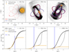 |
Fig. 1 Example of the satellite orbital and mass evolution. Upper panels: satellite particles of an example run featuring a satellite with as = 0.5 kpc, orbiting in the galactic plane of an exponential disc host, with initial velocity vi = 0.5 vc. From left to right, the three panels correspond to the first, middle, and final snapshot of the simulation. The origin coincides with the centre of the host galaxy potential. The colours indicate which particles are bound to the satellite (orange) or unbound (grey). The shaded red line shows the trajectory predicted by the semi-analytical model, while the solid red and blue lines track the satellite CoM, in the semi-analytical model and in the N-body simulation, respectively. Finally, the red cross indicates the initial point for the semi-analytical orbital integration, corresponding to the first apocentre. Lower panels: satellite cumulative mass profiles at the same snapshots and for the same system as in the upper panels. The solid black curve displays the theoretical cumulative mass profile from the Hernquist model. The other two profiles are constructed using the bound particles only (in orange) and all the particles that were part of the satellite at the initial time (in grey). The vertical blue line shows the value of the tidal radius computed with our semi-analytical prescription. |
3 Results
3.1 Models without dynamical friction
To test the efficiency of our semi-analytical model in predicting the evolution of a satellite galaxy within a non-spherical host, we started our investigation by considering the limiting case of a satellite moving in the analytical potential of a single-component disc-like host galaxy. Although far from realistic, this configuration allowed us to isolate the effects determined by tidal forces exerted only by the disc, excluding the influence of other factors that could have affected its orbital evolution, such as the presence of a spherical component in the host galaxy and the effect of DF.
Figure 3 displays the optimal values of the α parameter for each model, evaluated as detailed in Sect. 2.6. More in detail, the three panels show how the αbest parameter changes with the initial orbital velocity (or initial eccentricity) in models sharing the same satellite scale radius as, each panel referring to a different value of as, and the same orbital inclination, reported with different line styles and colours. In general, most systems exhibit a slight increase in the α parameter as the initial velocity approaches the circular velocity, while no evident trends in the values of α can be outlined when varying the scale radius and the orbital inclination. As expected, a lower α is associated with systems with initial higher eccentricity (or lower initial velocity). This is attributed to the abrupt decrease in the tidal radius at peri-centre passages, as predicted by Eq. (5), leading to a significant and instantaneous mass loss. However, the actual timescale to strip material from the satellite, as predicted by N-body simulations, is longer than the fast pericentre passages. For this reason, in the vicinity of the pericentre, the tidal radius decrease was delayed using Eq. (6), with α regulating the rapidity of the mass removal. Since this effect is much more relevant along eccentric orbits, the α parameter needs to be small enough to slow down the satellite mass loss, which otherwise would be extreme, and is expected to be smaller compared to systems with low eccentric orbits. If not explicitly specified, all the results presented from this point forwards refer to the specific semi-analytical model characterised by the optimal value of α for each system considered.
In Fig. 4 we present the results of the comparison between our semi-analytical prescription and N-body simulations for models with the satellite moving within the galactic plane. The upper panels depict the evolution of the separation of the satellite CoM from the primary galaxy centre. The semi-analytical model’s predictions are shown in orange, while the N-body simulation results are represented by a solid black line. The bottom panels show the time evolution of the difference between the satellite mass (normalised to the initial satellite mass) predicted by the semi-analytical model and the mass resulting from N-body simulations. The three panels correspond to different initial velocities of the satellite, with line colours indicating the satellite scale radius. Our semi-analytical prescription reproduces both the orbital and the mass evolution of the satellite well.
As an additional test, we compared our semi-analytical prescription for the tidal radius and mass evolution (solid lines) with results obtained using King’s formula (dashed lines; see Eq. (1)). We observe an overall better agreement with N-body simulations using our new semi-analytical prescription compared to the King prescription. This result is due to multiple factors. First, King’s formula, when applied without any delay for mass removal, implies instantaneous mass stripping. This leads to a general underestimation of the satellite mass, especially in the initial phases of the evolution. Moreover, one of the main assumptions in King’s prescription is that the tidal radius should be much lower than the separation between the centres of the two galaxies, thereby excluding close encounters. This assumption is generally valid along quasi-circular orbits, but it breaks when considering highly eccentric orbits where the pericentre can be at a close distance from the host centre. The combined effect of the instantaneous mass stripping, which can be severe in eccentric orbits during the close pericentre passages, and the assumption of distant interactions, imply an increasing inability of King’s prescription at reproducing the results of N-body simulations (see bottom-right panel in Fig. 4).
It is important to note that a comparison with King’s prescription is meaningful only for systems in which the satellite is orbiting within the galactic plane, as far from the galactic plane King’s definition of the tidal radius becomes ill-defined. In the co-planar case, indeed, the gradient of the host potential at the position of each satellite’s star points approximately towards the host centre, making the comparison between our and King’s prescriptions meaningful. Nonetheless, we stress that, even in this case, the acceleration of stars that during their orbits around the satellite centre lie above or below the plane of the host disc is not radial and is therefore, implicitly approximated in the treatment by King (1962).
Finally, we investigated systems where the satellite orbits outside the galactic plane, exploring various inclination angles. Since the qualitative trends observed in these cases are similar to the ones discussed for co-planar orbits, we show the evolution of the error in estimating the satellite mass for these systems in Fig. A.1.
Our semi-analytical prescription effectively reproduces the evolution of the satellite mass along the orbit, particularly in systems with eccentric orbits, across all orbital inclinations. However, in systems hosting satellites with low-eccentricity orbits, our semi-analytical model tends to overestimate the satellite mass, as observed in the right panels of Figs. 4 and A.1. We delve into this behaviour extensively in Section 3.3.
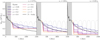 |
Fig. 2 Evolution of the satellite mass as a function of time for three cases with as = 0.5 kpc, orbiting within the host galactic plane and with different initial velocities (vi/vc = 0.75, 0.5, 0.25, from left to right). The black line shows the evolution of the mass according to the N-body simulations. The solid coloured lines correspond to the mass evolution predicted by the semi-analytical model with different values for α, spanning the range [0.05 − 5]. The dashed grey line represents the mass predicted using the minimum tidal radius evaluated along the 1000 different directions – if let free to increase –, whereas the grey region represents the time from the beginning of the N-body simulation to the first apocentre, which is the starting point for the semi-analytical models. |
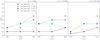 |
Fig. 3 Optimal values of the α parameter for each model without DF as a function of the initial orbital velocity (or initial eccentricity). Each panel considers a system with fixed satellite scale radius as, decreasing from left to right, with varying line styles and colour codes indicating different orbital inclinations. |
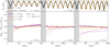 |
Fig. 4 Results obtained for systems hosing satellites orbiting within the galactic plane without DF. The three panels refers to different initial velocities for the satellite CoM, vi = 0.75, vi = 0.5 and vi = 0.25 form left to right. Upper panels: separation of the satellite CoM from the primary galaxy centre as a function of time. The thick dotted orange line refers to the semi-analytical model, while the thick solid black line shows the result of the N-body simulations. Bottom panels: time evolution of the difference between the satellite mass predicted by the semi-analytical model and the mass resulting from N-body simulations, normalised to the initial satellite mass. The line colours indicate different satellite scale radii. The solid lines refer to our new semi-analytical prescription for the evolution of the satellite mass, whereas the dashed lines represent the results we obtain using King’s formula for the tidal radius. In both panels, the grey area indicates the time interval leading to the first apocentre. |
3.2 Models with dynamical friction
After assessing the capability of our model to replicate the effects of tidal stripping in a fixed analytical potential, we extended our analysis to include models where DF is considered. In this context, our study involves satellite galaxies orbiting within a multi-component host galaxy. As detailed in Table 1, the host galaxy in these models comprises a spherically symmetric DM halo, incorporated as an analytical potential in N-body simulations, and an exponential disc containing 107 stellar particles. Consequently, the DF experienced by the satellite stars is solely attributed to the disc component of the host galaxy. In contrast to the models examined thus far, the introduction of DF, as described in detail in the introduction, significantly influences the satellite’s orbital evolution, which, in turn, plays a crucial role in shaping the tidal radius and consequently determining the extent of mass removal.
The combined effect of DF and mass loss is illustrated in Figure 5, where we report the result for one of the systems we tested (i.e. a satellite orbiting within the galactic plane with initial velocity of vi = 0.25vc and as = 0.5 kpc4). The left panels compare the satellite’s distance evolution from the centre of the host in the N-body simulation (depicted by the black line) with our semi-analytical model’s predictions for three distinct α values (each represented by a solid coloured line in a separate panel). Correspondingly, the right panel shows the satellite’s mass evolution in both N-body simulations and semi-analytical models, maintaining the same colour code as in the left panels.
In the right panel of Fig. 5, similarly to Figs. 2 and 6, it is possible to notice small increases in the satellite mass, occurring just after pericentre passages. Those increases are due to satellite particles that are stripped during the pericentre passage but, thanks to their orbital motion, are re-accreted soon after the closest approach to the host centre, rebinding to the satellite. The amount of matter re-accreted is very small compared to the amount of matter that one would predict to rebind to the satellite after each pericentre passage in the case of a freely evolving Rt (dashed grey line). For this reason, and also the fact that the amplitude of this bump in the satellite mass gets damped with the subsequent pericentre passages, we neglected this effect and considered the Rt to be a decreasing function of time.
Among the models investigated, the one corresponding to α = 0.1 exhibits the best agreement with both the satellite’s mass and orbital evolution. Conversely, models associated with higher values of α, corresponding to faster mass loss, demonstrate an increasing deviation from simulations results. This discrepancy arises from the rapid reduction in the satellite mass, which leads to a weakening of the DF drag, consequently slowing down the satellite’s decay towards the host centre.
The best values of the α parameter for all the investigated systems are summarised in Table 2. As highlighted in the previous section, models devoid of DF exhibit a consistent agreement between our semi-analytical model and N-body simulations, independently of the scale radius and orbital inclination, with a mild dependence on the initial orbital eccentricity only. Given this result, and the fact that simulations involving a host disc composed of 107 particles represent a quite high computational burden compared to simulations with entirely analytical hosts, we opted to focus our investigation on systems featuring a satellite with a fixed scale radius, as = 0.5 kpc, orbiting within the galactic plane. The primary parameter under consideration is therefore the variation in the satellite’s initial velocity.
The results are shown in Fig. 7. The left panels compare the evolution of the satellite’s CoM in both simulations and in semianalytical models, each using the best value for α. From top to bottom, the different panels correspond to the three different initial satellite’s velocities, vi = 0.75vc, vi = 0.50vc and vi = 0.25vc. The right panel depicts the error in the evaluation of the satellite mass for the same values of the initial velocities.
As noted in the previous cases, a very good agreement is observed between the results obtained from N-body simulations and the predictions from our semi-analytical models regarding the orbital evolution of the satellite and the associated mass decrease. Notably, this accord is particularly pronounced for systems featuring satellites on higher eccentric orbits, as consistently demonstrated across all the investigated systems.
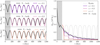 |
Fig. 5 Orbital and mass evolution of a satellite when the effect of DF is included. Left panels: time-evolution of the satellite’s distance from the centre of the host in the N-body simulation (black lines) compared to our semi-analytical model’s predictions (solid coloured lines). From top to bottom, each panel refers to different values of α: 0.1, 0.2, and 1, respectively. Right panel: mass evolution of the satellite in both N-body simulations and semi-analytical models, maintaining the same colour code as in the left panels. The dashed grey line represents the mass predicted using the minimum tidal radius evaluated along the 1000 different directions – if let free to increase. |
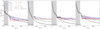 |
Fig. 6 Satellite mass as a function of time for systems with the re-orientation of the satellite star velocities at the apocentres. The four panels refer to different orbital inclinations, from θ = 0 (leftmost panel) to θ = π/2 (rightmost panel). The dashed black line represents the satellite mass obtained through the new N-body simulations, compared with the outcome of the original N-body simulations shown as a solid black line. The coloured lines indicate the predictions of our semi-analytical model for various values of α. The dashed grey line represents the mass predicted using the minimum tidal radius evaluated along the 1000 different directions – if let free to increase. |
Values of the α parameter for each model in this work.
3.3 Testing low-eccentricity satellite orbits
In this section, we investigate in detail the processes contributing to the systematic overestimation of satellite mass in our semi-analytical model when compared to N-body simulations in systems harbouring satellites on low-eccentricity orbits. Two primary processes may account for this discrepancy. The first involves tidal heating resulting from rapid changes in the host potential experienced by the satellite, as described at the beginning of the methods. Another possible factor is the satellite’s evaporation induced by mass truncation. During pericentre passages, where the majority of stripping occurs, a substantial portion of the satellite mass is expelled from the system, leading to truncation in the satellite mass distribution. As a result, the satellite is no longer in equilibrium. As it evolves towards a new equilibrium, its mass distribution expands, causing stars with higher velocities to migrate to larger radii. As a consequence, the satellite’s profile changes becoming less concentrated, thereby facilitating the particles in the outer layers to become unbound. This results in a continuous mass loss, even if the tidal radius undergoes minimal change, particularly along quasi-circular orbits.
In order to discern the predominant process influencing the excess mass loss in the satellite, we conducted additional N-body simulations without DF. This was done to exclude potential additional effects that could contribute to the removal of mass from the satellite. The simulations were executed considering only systems characterised by the lowest initial orbital eccentricity, specifically with vi = 0.75vc, as these are the most affected by the process under investigation. The satellite under consideration features a Hernquist mass distribution with as = 0.5. Instead of randomly oriented velocities, we initialised stars in the satellite on perfectly circular orbits, ensuring that no net rotation was imparted to the satellite as a whole.
To deal with the tendency of the velocities of the satellite stars to re-isotropise, a re-orientation of the particles’ velocities along the tangential direction was performed at every apocentre. Importantly, this re-orientation did not alter the magnitude of the velocity vector, thus keeping the energies of the stars unchanged. This approach prevents stars on radial orbits from rapidly migrating towards larger radii, thereby restraining the overall evaporation of the satellite. This approach enables the discrimination between the processes driving the excess in satellite mass loss. If the dominant factor is satellite evaporation, this methodology allows the satellite mass evolution to be reproduced. Alternatively, if tidal heating is the primary driver, injecting energy into the satellite and causing the stars to acquire sufficient energy to escape the system, our simulation will still exhibit an excess in mass loss.
The results are shown in Fig. 6. Each panel illustrates the satellite mass as a function of time for distinct orbital inclinations. In all systems, a substantial reduction in the mass loss rate is observed. Notably, the system harbouring a satellite orbiting within the galactic plane exhibits a satellite mass evolution now compatible with our semi-analytical model, particularly for α = 0.05. Conversely, in systems with orbits outside the galactic plane, although the reduction in satellite mass is more gradual compared to the original N-body runs, the stripped mass still exceeds that predicted by the semi-analytical models. This suggests that, at least within the galactic plane, the re-orientation of star velocities is sufficient to reconcile the evolution with the semi-analytical model, indicating the dominance of satellite evaporation in shaping the mass evolution. Outside the galactic plane, however, tidal heating effects become significant, due to the stronger vertical gradient of the gravitational field in the proximity of the disc plane, and therefore it cannot be neglected.
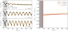 |
Fig. 7 Comparison between the outcomes of N-body simulations and our semi-analytical model in systems with DF. Left panels: comparison between the evolution of the satellite’s CoM in both N-body simulations and semi-analytical models, each using the best value for α. The different panels correspond to the three different initial satellite’s velocities, vi = 0.75vc, vi = 0.50vc and vi = 0.25vc from top to bottom. The thick dotted orange line refers to the semi-analytical model, while the thick solid black line shows the result of the N-body simulations. Right panel: relative error in the evaluation of the satellite mass for the same values of the initial velocities as a function of time. Different line colours indicate different initial satellite velocities. The dashed vertical lines represent the initial time of the semi-analytical models, which corresponds to the first apocentre, and are coloured using the same colour code employed for the solid lines. |
4 Discussion and conclusions
In our analysis we evolved a satellite galaxy within a fixed (or quasi-fixed, for the simulations with live primaries) host potential. However, galaxies experience morphological evolution throughout cosmic time due to secular evolution. This evolutionary process can result from interactions between the galaxy and its environment, such as gas accretion or galaxy harassment, or it can be initiated by internal factors such as the presence of spiral arms or bars. Analysing cosmological simulations Santistevan et al. (2023); Santistevan et al. (2024) show that the growth of galaxies and their DM halos on sub-gigayear scales can significantly impact the evolution of merging satellite galaxies, especially affecting the satellite orbit during the pairing phase and, consequently, its infall time. Such a result is indeed backed up by analytical arguments, such as those described in Volonteri et al. (2020). Interestingly, and contrary to what is commonly expected, Santistevan et al. (2023); Santistevan et al. (2024) find that the satellite orbit is not always shrinking. Instead, some satellites exhibit an increase in the pericentre distance, often accompanied by a rise in the orbital specific angular momentum. This suggests that the growth of the host galaxy halo may promote the satellite migration to larger orbits, thus exerting a strong influence on its evolution. In light of these considerations, we have started applying our model to galaxies undergoing significant evolution, thus relaxing the constraint of a static primary galaxy potential dictating the motion of the satellite and allowing for both galaxies to evolve over time and pair together. The results of this analysis will be discussed in a forthcoming study.
In our study, we focused on the stellar and DM component of the merging galaxies, while we neglected the presence of gas in the merging galaxies. Our choice was motivated by our primary goal of characterising the tidal stripping of satellite galaxies in non-spherical hosts rather than a full inclusion of the different galactic components. Nevertheless, concerning minor mergers, cosmological simulations show that these events can involve gasrich satellites interacting with the gaseous component of their host (see e.g. Moreno et al. 2022). In such cases, the effects of ram pressure and of non-axisymmetric torques on the gas component crucially impact the DF efficiency. On one hand, by removing mass from the satellite galaxy (Abadi et al. 1999; Mayer et al. 2006; Samuel et al. 2022, 2023), ram pressure slows the satellite orbital evolution. On the other hand, Callegari et al. (2009) show that gas inflows triggered by non-axisymmetric structures5 driven by the merger process stabilise the satellite nucleus against tidal disruption, leading to the successful completion of MBH pairing in unequal (1:10) galaxy mergers, while similar gas-free simulations resulted in the wandering of the smallest MBH at kiloparsec scales. We plan to address these effects on the efficiency of DF and tidal stripping in gas-rich mergers in a future study.
Finally, we performed our study considering a single satellite-to-host mass ratio of <1:100. Increasing the mass ratio would introduce significant distortions in the host potential, thus requiring dedicated studies and simulations that account for variations in the host potential and mass distribution.
In this paper, we proposed a new semi-analytical prescription for the tidal radius and the relative mass evolution of satellite galaxies in minor mergers. The novelty of the proposed approach primarily lies in the generalisation of the definition of the tidal radius such that it is suitable for any geometry and composition of the host galaxy, in contrast with the traditional definitions (King 1962) that are provided for circular orbits under the assumption of a spherical host. The prescription also accounts for a delay in the mass stripping and allows for eccentric orbits.
We validated our prescription against N-body simulations. To isolate the effects of tidal forces, we first considered systems not affected by DF, by considering a spherically symmetric satellite orbiting within the analytical potential of an exponential-disc host. We explored the parameter space by considering different initial orbital velocities, orbital inclinations, and satellite scale radii.
For each tested system, we selected the semi-analytical evolution characterised by the α parameter that best reproduces the mass evolution of the satellite in N-body simulations. Such a parameter regulates the rapidity of mass loss in our semi-analytical model, with higher values related to faster mass loss. We find a mild dependence of the best α with the initial orbital velocity, while no significant dependences with the satellite scale radius and orbital inclination are observed. Lower values of α are associated with more eccentric orbits, reflecting the need for a larger delay in mass loss due to faster pericentre passages.
Our model demonstrated excellent agreement with N-body simulations, accurately reproducing the satellite mass evolution, especially for systems with mildly and highly eccentric orbits. However, for systems with initial velocities close to vc, a slight systematic overestimation of the satellite mass loss was observed.
This mass loss excess observed in systems with satellites on low-eccentricity orbits is likely influenced by two primary processes: tidal heating and satellite evaporation induced by mass truncation. To delve into this discrepancy, we ran additional N-body simulations, where at each apocentre a re-orientation of star velocities along the tangential direction was performed. In systems where the satellite orbits within the galactic plane, the re-orientation of star velocities mitigates the excess mass loss, aligning the simulation results with the predictions of our semi-analytical model. This suggests that, within the galactic plane, together with tidal stripping, satellite evaporation plays a dominant role in shaping the mass evolution. Still, outside the galactic plane, the reduction in excess mass loss is milder, and tidal heating effects become significant. This indicates that, in these configurations, both tidal heating and satellite evaporation contribute to the observed discrepancies between N-body simulations and the semi-analytical model.
Moreover, for orbits within the galactic plane, we compared our semi-analytical prescription for the satellite mass evolution with the instantaneous mass loss predicted using King’s formula in reproducing the results of N-body simulations. We find that our model better reproduces the mass evolution in the simulations. It is important to stress that outside the galactic plane – and in general in every non-central potential – King’s tidal radius is not well defined.
We then considered systems with both tidal stripping and DF effects. The semi-analytical model accurately reproduces both the orbital evolution and mass loss of the satellite.
These findings provide valuable insights into the complex interplay of tidal forces, DF, and the orbital parameters of satellite galaxies. Understanding these processes is crucial for accurately modelling the evolution of satellite galaxies within their host galactic environments.
Acknowledgements
We thank David Izquierdo-Villalba, Pedro Capelo, Lucio Mayer and Eugene Vasiliev for valuable discussions and suggestions. MB acknowledges support provided by MUR under grant “PNRR – Missione 4 Istruzione e Ricerca – Componente 2 Dalla Ricerca all’Impresa – Investimento 1.2 Finanziamento di progetti presentati da giovani ricercatori ID:SOE_0163” and by University of Milano-Bicocca under grant “2022-NAZ-0482/B”. LV aknowledges support from MIUR under the grant PRIN 2017-MB8AEZ. AL acknowledges support by the PRIN MUR “2022935STW”. E.B. acknowledges the financial support provided under the European Union’s H2020 ERC Consolidator Grant “Binary Massive Black Hole Astrophysics” (B Massive, Grant Agreement: 818691). E.B. acknowledges support from the European Union’s Horizon Europe programme under the Marie Skłodowska-Curie grant agreement No 101105915 (TESIFA).
Appendix A Systems with orbits outside the galactic plane
In this section, we present the results for the systems with the satellite galaxy orbiting outside the galactic plane. The columns represent different initial velocities of the satellite CoM, decreasing from left to right, while the rows illustrate varying orbital inclinations, increasing in angle from top to bottom.
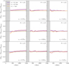 |
Fig. A.1 Error in estimating the satellite mass for systems on inclined orbits with respect to the galactic plane and without DF. The line colours indicate different satellite scale radii. The columns represent different initial velocities of the satellite CoM, decreasing from left to right, while the rows illustrate varying orbital inclinations, increasing in angle from top to bottom. |
References
- Abadi, M. G., Moore, B., & Bower, R. G. 1999, MNRAS, 308, 947 [Google Scholar]
- Agazie, G., Anumarlapudi, A., Archibald, A. M., et al. 2023, ApJ, 951, L8 [NASA ADS] [CrossRef] [Google Scholar]
- Amaro-Seoane, P., Audley, H., Babak, S., et al. 2017, arXiv e-prints [arXiv:1702.00786] [Google Scholar]
- Antoniadis, J., Arumugam, P., Arumugam, S., et al. 2023, A&A, 678, A50 [CrossRef] [EDP Sciences] [Google Scholar]
- Begelman, M. C., Blandford, R. D., & Rees, M. J. 1980, Nature, 287, 307 [Google Scholar]
- Bernardi, M., Sheth, R. K., Annis, J., et al. 2003, AJ, 125, 1817 [NASA ADS] [CrossRef] [Google Scholar]
- Binney, J., & Tremaine, S. 1987, Galactic dynamics (Princeton: Princeton University Press) [Google Scholar]
- Blumenthal, K. A., & Barnes, J. E. 2018, MNRAS, 479, 3952 [Google Scholar]
- Bonetti, M., Sesana, A., Barausse, E., & Haardt, F. 2018, MNRAS, 477, 2599 [NASA ADS] [CrossRef] [Google Scholar]
- Bonetti, M., Bortolas, E., Lupi, A., Dotti, M., & Raimundo, S. I. 2020, MNRAS, 494, 3053 [NASA ADS] [CrossRef] [Google Scholar]
- Bonetti, M., Bortolas, E., Lupi, A., & Dotti, M. 2021, MNRAS, 502, 3554 [NASA ADS] [CrossRef] [Google Scholar]
- Bortolas, E., Bonetti, M., Dotti, M., et al. 2022, MNRAS, 512, 3365 [NASA ADS] [CrossRef] [Google Scholar]
- Bottrell, C., Yesuf, H. M., Popping, G., et al. 2024, MNRAS, 527, 6506 [Google Scholar]
- Bournaud, F., Jog, C. J., & Combes, F. 2007, A&A, 476, 1179 [NASA ADS] [CrossRef] [EDP Sciences] [Google Scholar]
- Buitrago, F., Conselice, C. J., Epinat, B., et al. 2014, MNRAS, 439, 1494 [NASA ADS] [CrossRef] [Google Scholar]
- Callegari, S., Mayer, L., Kazantzidis, S., et al. 2009, ApJ, 696, L89 [NASA ADS] [CrossRef] [Google Scholar]
- Callegari, S., Kazantzidis, S., Mayer, L., et al. 2011, ApJ, 729, 85 [NASA ADS] [CrossRef] [Google Scholar]
- Capelo, P. R., & Dotti, M. 2017, MNRAS, 465, 2643 [Google Scholar]
- Chandrasekhar, S. 1943, ApJ, 97, 255 [Google Scholar]
- Conselice, C. J., Bluck, A. F. L., Mortlock, A., Palamara, D., & Benson, A. J. 2014, MNRAS, 444, 1125 [Google Scholar]
- Cox, T. J., Jonsson, P., Somerville, R. S., Primack, J. R., & Dekel, A. 2008, MNRAS, 384, 386 [NASA ADS] [CrossRef] [Google Scholar]
- Dekel, A., Sari, R., & Ceverino, D. 2009, ApJ, 703, 785 [Google Scholar]
- Ferrarese, L., & Ford, H. 2005, Space Sci. Rev., 116, 523 [Google Scholar]
- Gajda, G., & Łokas, E. L. 2016, ApJ, 819, 20 [NASA ADS] [CrossRef] [Google Scholar]
- Henon, M. 1970, A&A, 9, 24 [NASA ADS] [Google Scholar]
- Hernquist, L. 1990, ApJ, 356, 359 [Google Scholar]
- Hilz, M., Naab, T., Ostriker, J. P., et al. 2012, MNRAS, 425, 3119 [Google Scholar]
- Hopkins, P. F., Somerville, R. S., Cox, T. J., et al. 2009, MNRAS, 397, 802 [NASA ADS] [CrossRef] [Google Scholar]
- Jackson, R. A., Martin, G., Kaviraj, S., et al. 2019, MNRAS, 489, 4679 [NASA ADS] [CrossRef] [Google Scholar]
- Kaviraj, S. 2014, MNRAS, 440, 2944 [Google Scholar]
- Kazantzidis, S., Kravtsov, A. V., Zentner, A. R., et al. 2004, ApJ, 611, L73 [Google Scholar]
- Keenan, D. W., & Innanen, K. A. 1975, Celest. Mech., 11, 85 [Google Scholar]
- King, I. 1962, AJ, 67, 471 [Google Scholar]
- Kormendy, J., & Ho, L. C. 2013, ARA&A, 51, 511 [Google Scholar]
- Kumar, A., More, S., & Sunayama, T. 2024, arXiv e-prints [arXiv:2312.04847v1] [Google Scholar]
- Martin, G., Kaviraj, S., Devriendt, J. E. G., Dubois, Y., & Pichon, C. 2018, MNRAS, 480, 2266 [Google Scholar]
- Mayer, L., Mastropietro, C., Wadsley, J., Stadel, J., & Moore, B. 2006, MNRAS, 369, 1021 [NASA ADS] [CrossRef] [Google Scholar]
- Moreno, J., Torrey, P., Ellison, S. L., et al. 2021, MNRAS, 503, 3113 [NASA ADS] [CrossRef] [Google Scholar]
- Moreno, J., Danieli, S., Bullock, J. S., et al. 2022, Nat. Astron., 6, 496 [NASA ADS] [CrossRef] [Google Scholar]
- Navarro, J. F., Frenk, C. S., & White, S. D. M. 1997, ApJ, 490, 493 [Google Scholar]
- Neumayer, N., Seth, A., & Böker, T. 2020, A&A Rev., 28, 4 [NASA ADS] [CrossRef] [Google Scholar]
- Pace, C., & Salim, S. 2014, ApJ, 785, 66 [NASA ADS] [CrossRef] [Google Scholar]
- Press, W. H., & Schechter, P. 1974, ApJ, 187, 425 [Google Scholar]
- Qu, Y., Di Matteo, P., Lehnert, M. D., van Driel, W., & Jog, C. J. 2011, A&A, 535, A5 [NASA ADS] [CrossRef] [EDP Sciences] [Google Scholar]
- Read, J. I., Wilkinson, M. I., Evans, N. W., Gilmore, G., & Kleyna, J. T. 2006, MNRAS, 366, 429 [NASA ADS] [CrossRef] [Google Scholar]
- Reardon, D. J., Zic, A., Shannon, R. M., et al. 2023, ApJ, 951, L6 [NASA ADS] [CrossRef] [Google Scholar]
- Renaud, F., Boily, C. M., Naab, T., & Theis, C. 2009, ApJ, 706, 67 [NASA ADS] [CrossRef] [Google Scholar]
- Samuel, J., Wetzel, A., Santistevan, I., et al. 2022, MNRAS, 514, 5276 [NASA ADS] [CrossRef] [Google Scholar]
- Samuel, J., Pardasani, B., Wetzel, A., et al. 2023, MNRAS, 525, 3849 [NASA ADS] [CrossRef] [Google Scholar]
- Santistevan, I. B., Wetzel, A., Tollerud, E., Sanderson, R. E., & Samuel, J. 2023, MNRAS, 518, 1427 [Google Scholar]
- Santistevan, I. B., Wetzel, A., Tollerud, E., et al. 2024, MNRAS, 527, 8841 [Google Scholar]
- Shibuya, T., Ouchi, M., & Harikane, Y. 2015, ApJS, 219, 15 [Google Scholar]
- Smith, S. E. T., Cerny, W., Hayes, C. R., et al. 2024, arXiv e-prints [arXiv:2311.10147] [Google Scholar]
- Springel, V., Pakmor, R., Zier, O., & Reinecke, M. 2021, MNRAS, 506, 2871 [NASA ADS] [CrossRef] [Google Scholar]
- Taranu, D. S., Dubinski, J., & Yee, H. K. C. 2013, ApJ, 778, 61 [NASA ADS] [CrossRef] [Google Scholar]
- van den Bosch, F. C., & Ogiya, G. 2018, MNRAS, 475, 4066 [NASA ADS] [CrossRef] [Google Scholar]
- Ventou, E., Contini, T., Bouché, N., et al. 2019, A&A, 631, A87 [NASA ADS] [CrossRef] [EDP Sciences] [Google Scholar]
- Volonteri, M., Haardt, F., & Madau, P. 2003, ApJ, 582, 559 [Google Scholar]
- Volonteri, M., Pfister, H., Beckmann, R. S., et al. 2020, MNRAS, 498, 2219 [Google Scholar]
- von Hoerner, S. 1957, ApJ, 125, 451 [NASA ADS] [CrossRef] [Google Scholar]
- White, S. D. M., & Rees, M. J. 1978, MNRAS, 183, 341 [Google Scholar]
- Yurin, D., & Springel, V. 2014, MNRAS, 444, 62 [NASA ADS] [CrossRef] [Google Scholar]
See however Jackson et al. (2019), who demonstrate that single minor merger events involving systems with mass ratios ~0.1–0.3, and with the satellite moving on orbits almost aligned with the host’s disc plane, may trigger catastrophic changes in the primary morphology within timescales as short as a few hundred megayears.
Here, we refer to the total potential of the primary galaxy, composed of both baryonic and DM components. If one focuses on the DM halo, the work of Kazantzidis et al. (2004) show that baryonic cooling and the formation of a disc can enhance symmetry in the inner regions of halos.
The criteria in van den Bosch & Ogiya (2018) were computed assuming a Navarro-Frenk-White (Navarro et al. 1997) profile for the satellite galaxy. We applied these criteria to our satellites, even though our analysis employed a Hernquist model. Extending the computation to determine the precise threshold for a Hernquist profile is beyond the scope of this paper.
Due to the computational cost of simulations involving a high number of particles, and since the results of simulations without DF are almost independent of the satellite scale radius, we chose to consider a single value for as. We picked as = 0.5 kpc, namely the middle value among those that we tested in the previous sections.
Similar inflow can be triggered by the ram pressure torques as well (see e.g. Capelo & Dotti 2017; Blumenthal & Barnes 2018).
All Tables
Parameters of the host galaxy for both the single- and double-component scenarios.
All Figures
|
Fig. 1 Example of the satellite orbital and mass evolution. Upper panels: satellite particles of an example run featuring a satellite with as = 0.5 kpc, orbiting in the galactic plane of an exponential disc host, with initial velocity vi = 0.5 vc. From left to right, the three panels correspond to the first, middle, and final snapshot of the simulation. The origin coincides with the centre of the host galaxy potential. The colours indicate which particles are bound to the satellite (orange) or unbound (grey). The shaded red line shows the trajectory predicted by the semi-analytical model, while the solid red and blue lines track the satellite CoM, in the semi-analytical model and in the N-body simulation, respectively. Finally, the red cross indicates the initial point for the semi-analytical orbital integration, corresponding to the first apocentre. Lower panels: satellite cumulative mass profiles at the same snapshots and for the same system as in the upper panels. The solid black curve displays the theoretical cumulative mass profile from the Hernquist model. The other two profiles are constructed using the bound particles only (in orange) and all the particles that were part of the satellite at the initial time (in grey). The vertical blue line shows the value of the tidal radius computed with our semi-analytical prescription. |
| In the text | |
|
Fig. 2 Evolution of the satellite mass as a function of time for three cases with as = 0.5 kpc, orbiting within the host galactic plane and with different initial velocities (vi/vc = 0.75, 0.5, 0.25, from left to right). The black line shows the evolution of the mass according to the N-body simulations. The solid coloured lines correspond to the mass evolution predicted by the semi-analytical model with different values for α, spanning the range [0.05 − 5]. The dashed grey line represents the mass predicted using the minimum tidal radius evaluated along the 1000 different directions – if let free to increase –, whereas the grey region represents the time from the beginning of the N-body simulation to the first apocentre, which is the starting point for the semi-analytical models. |
| In the text | |
|
Fig. 3 Optimal values of the α parameter for each model without DF as a function of the initial orbital velocity (or initial eccentricity). Each panel considers a system with fixed satellite scale radius as, decreasing from left to right, with varying line styles and colour codes indicating different orbital inclinations. |
| In the text | |
|
Fig. 4 Results obtained for systems hosing satellites orbiting within the galactic plane without DF. The three panels refers to different initial velocities for the satellite CoM, vi = 0.75, vi = 0.5 and vi = 0.25 form left to right. Upper panels: separation of the satellite CoM from the primary galaxy centre as a function of time. The thick dotted orange line refers to the semi-analytical model, while the thick solid black line shows the result of the N-body simulations. Bottom panels: time evolution of the difference between the satellite mass predicted by the semi-analytical model and the mass resulting from N-body simulations, normalised to the initial satellite mass. The line colours indicate different satellite scale radii. The solid lines refer to our new semi-analytical prescription for the evolution of the satellite mass, whereas the dashed lines represent the results we obtain using King’s formula for the tidal radius. In both panels, the grey area indicates the time interval leading to the first apocentre. |
| In the text | |
|
Fig. 5 Orbital and mass evolution of a satellite when the effect of DF is included. Left panels: time-evolution of the satellite’s distance from the centre of the host in the N-body simulation (black lines) compared to our semi-analytical model’s predictions (solid coloured lines). From top to bottom, each panel refers to different values of α: 0.1, 0.2, and 1, respectively. Right panel: mass evolution of the satellite in both N-body simulations and semi-analytical models, maintaining the same colour code as in the left panels. The dashed grey line represents the mass predicted using the minimum tidal radius evaluated along the 1000 different directions – if let free to increase. |
| In the text | |
|
Fig. 6 Satellite mass as a function of time for systems with the re-orientation of the satellite star velocities at the apocentres. The four panels refer to different orbital inclinations, from θ = 0 (leftmost panel) to θ = π/2 (rightmost panel). The dashed black line represents the satellite mass obtained through the new N-body simulations, compared with the outcome of the original N-body simulations shown as a solid black line. The coloured lines indicate the predictions of our semi-analytical model for various values of α. The dashed grey line represents the mass predicted using the minimum tidal radius evaluated along the 1000 different directions – if let free to increase. |
| In the text | |
|
Fig. 7 Comparison between the outcomes of N-body simulations and our semi-analytical model in systems with DF. Left panels: comparison between the evolution of the satellite’s CoM in both N-body simulations and semi-analytical models, each using the best value for α. The different panels correspond to the three different initial satellite’s velocities, vi = 0.75vc, vi = 0.50vc and vi = 0.25vc from top to bottom. The thick dotted orange line refers to the semi-analytical model, while the thick solid black line shows the result of the N-body simulations. Right panel: relative error in the evaluation of the satellite mass for the same values of the initial velocities as a function of time. Different line colours indicate different initial satellite velocities. The dashed vertical lines represent the initial time of the semi-analytical models, which corresponds to the first apocentre, and are coloured using the same colour code employed for the solid lines. |
| In the text | |
|
Fig. A.1 Error in estimating the satellite mass for systems on inclined orbits with respect to the galactic plane and without DF. The line colours indicate different satellite scale radii. The columns represent different initial velocities of the satellite CoM, decreasing from left to right, while the rows illustrate varying orbital inclinations, increasing in angle from top to bottom. |
| In the text | |
Current usage metrics show cumulative count of Article Views (full-text article views including HTML views, PDF and ePub downloads, according to the available data) and Abstracts Views on Vision4Press platform.
Data correspond to usage on the plateform after 2015. The current usage metrics is available 48-96 hours after online publication and is updated daily on week days.
Initial download of the metrics may take a while.