| Issue |
A&A
Volume 689, September 2024
|
|
|---|---|---|
| Article Number | A174 | |
| Number of page(s) | 11 | |
| Section | Extragalactic astronomy | |
| DOI | https://doi.org/10.1051/0004-6361/202449676 | |
| Published online | 13 September 2024 | |
The radio properties of z > 3.5 quasars: Are most high-redshift radio-loud active galactic nuclei obscured?
INAF – Osservatorio Astrofisico di Torino, Strada Osservatorio 20, 10025 Pino Torinese, Italy
Received:
20
February
2024
Accepted:
19
June
2024
Abstract
We explore the radio properties of powerful (rest-frame luminosity ≳1028 W Hz−1 at 500 MHz) high-redshift (z ≳ 3.5) quasars. The aim of this study is to gain a better understanding of radio-loud sources at the epoch when they reach the highest space density. We selected 29 radio-loud quasars at low radio frequencies (76 MHz). Their radio spectra, covering the range from 76 MHz to 5 GHz, are generally well reproduced by a single power law. We created samples that were matched in radio luminosity at lower redshift (from z ∼ 1.3 to z ∼ 2.8) to investigate any spectral evolution. We find that the fraction of flat-spectrum radio quasars (FSRQs) strongly increases with redshift (from ∼8% at z = 1.2 to ∼45% at z > 3.5). This effect is also observed in quasars with lower luminosities (down to ∼1027 W Hz−1). The increase in the fraction of FSRQs with redshift corresponds to a decrease in the steep- spectrum radio quasars. This result can be explained when we assume that the beaming factor and the slope of the luminosity function do not change with redshift, if high-redshift radio-loud sources can be recognized as quasars only when they are seen at a small viewing angle (≲25°), while most of them, about 90%, are obscured in the UV and optical bands. We also found a trend for the size of radio sources to decrease with increasing redshift. Because projection effects are insufficient to cause this trend, we suggest that the large amount of gas causing the nuclear obscuration also hampers the growth of the more distant sources.
Key words: galaxies: active / galaxies: jets / quasars: general
Corresponding author; This email address is being protected from spambots. You need JavaScript enabled to view it.
© The Authors 2024
 Open Access article, published by EDP Sciences, under the terms of the Creative Commons Attribution License (https://creativecommons.org/licenses/by/4.0), which permits unrestricted use, distribution, and reproduction in any medium, provided the original work is properly cited.
This article is published in open access under the Subscribe to Open model. This email address is being protected from spambots. You need JavaScript enabled to view it. to support open access publication.
1. Introduction
Powerful radio-loud active galactic nuclei (RLAGN) represent the most extreme manifestation of activity powered by accretion onto supermassive black holes. They play a pivotal role in cosmology and galaxy evolution. Their host galaxies are, or are destined to become, massive giant elliptical galaxies, many of which are brightest cluster galaxies (see, e.g., Best et al. 2005; Miraghaei & Best 2017). The intense nuclear emission and highly collimated jets of RLAGN can profoundly influence the star formation, excitation, and ionization of the intra-cluster medium (ICM; e.g., Fabian 2012; Voit et al. 2015). Cosmological models that do not account for the radio mode AGN feedback lead to galaxy luminosities, colors, and disk and bulge sizes that disagree with observations (e.g., Croton et al. 2006).
At low redshift, z ≲ 1, the properties of radio sources are quite well understood (see Tadhunter 2016 for a review). In particular, it has been suggested that the observed variegated phenomenology can be understood within the unified model (UM) of radio AGN. The UM postulates that various classes of objects are intrinsically identical and differ only in their orientation with respect to our line of sight (see, e.g., Antonucci 1993 for a review). The origin of the observational differences is due to the presence of (i) circumnuclear absorbing material (usually referred to as the obscuring torus) that produces selective absorption when the source is observed at a large angle from its radio axis, and (ii) Doppler boosting, which is associated with relativistic motions in AGN jets.
In the unification scheme of RLAGN (e.g., Urry & Padovani 1995) narrow-lined radio galaxies of Fanaroff Riley (FR) type II (Fanaroff & Riley 1974) and broad-lined FR IIs together with RL QSOs are considered to be intrinsically indistinguishable. Their different aspect (in particular, the absence of broad emission lines in FR IIs) is only related to their orientation in the sky with respect to our line of sight. Therefore, in its stricter interpretation of a pure orientation scheme, the UM predicts that narrow- and broad-line FR II are drawn from the same parent population. According to this model, a source appears as a quasar stellar object (QSO) only when its radio axis is oriented within a small cone from the observer’s line of sight (Barthel 1989); conversely, when seen at large angles, the nuclear emission (including the broad-line region) is obscured, and they are called radio galaxies. Probably the most convincing of several pieces of evidence in favor of the UM is the detection of broad lines in the polarized spectra of narrow-line objects (Antonucci 1982, 1984), which was interpreted as the result of scattered light from an otherwise obscured nucleus. Although the UM is generally successful in explaining the variety of RLAGN behavior, some issues still remain to be explained. For example, the powerful FR II showing weak emission lines might represent evidence that in addition to the effect of orientation, changes in the accretion rate play an important role (see, e.g., Tadhunter et al. 1998).
Baldi et al. (2013) explored the properties of radio sources extracted from the third Cambridge catalog (3C, Spinrad et al. 1985) with z < 0.3 and found a fraction of narrow-line sources of ∼65%. In a torus geometry, this fraction corresponds to a torus opening angle of 50° ±5. Lawrence (1991), Hill et al. (1996), and Willott et al. (2000) found that the fraction of narrow-line objects decreases with increasing radio power. It reaches ∼50% for the most powerful sources at 1 < z < 2. The authors proposed that this is due to a lower covering factor of the circumnuclear absorption structure in the more luminous sources, the so-called receding torus model.
The UM has also successfully explained the observed properties of the sources in which the dominant effects of anisotropy are due to Doppler amplification of the emission of a relativistic jet oriented at a small angle with respect to our line of sight (see Urry & Padovani 1995 for a review). The highly amplified sources that form the class of blazars can be separated into two main classes depending on whether broad emission lines are visible in their optical spectra. In the first case, they are called flat-spectrum radio quasars (FSRQs; with a radio spectral index α < 0.5) and their observed radio emission originates mainly from the base of their relativistic jets when these are seen at a small angle from the line of sight. In the objects oriented at a larger angle, in which the amplification is not so extreme, the radio emission is ascribed to optically thin synchrotron radiation produced by large-scale regions. Therefore, they show a steep radio spectrum and are called steep-spectrum radio quasars (SSRQs).
The high-redshift range, z ≳ 3 − 4, is particularly important: The results of Caccianiga et al. (2019) and Lister et al. (2019) showed that the density of the most luminous RLAGN peaks at this epoch, when AGN feedback was more active. As already observed at low redshift, high-z RLAGN might also manifest as sources in which the nucleus is optically obscured, as in the case of high-redshift radio galaxies (HzRGs). The nucleus can instead be directly visible, as is the case in high-redshift radio quasars (HzRQs). HzRQs in turn might show both steep and flat spectra (e.g., Sotnikova et al. 2021), suggesting that the RLAGN unified scheme might also apply at high redshift.
However, our knowledge of the properties of RLAGN at high redshift is less detailed than it is for lower redshift objects. Only 19 HzRGs are contained in the list of optically obscured AGN at z > 3.5 in the list compiled by Miley & De Breuck (2008), and only a few more have been discovered since then (e.g., Saxena et al. 2018; Yamashita et al. 2020). Furthermore, the main programs of HzRG searches were carried out selecting ultrasteep radio sources (USS; e.g., De Breuck et al. 2006). USS were defined by Miley & Chambers (1989) as sources with a spectral index α > 1 (defined as fν ∝ ν−α). This criterion was motivated by the phenomenological trend that suggested that higher-redshift radio sources have steeper radio spectra (De Breuck et al. 2001), but it leads to a selection bias.
Conversely, large samples of quasars at high redshift are available. For example, there are ∼10 000 QSOs at z > 3.5 in the Sloan Digital Sky Survey (SDSS; York et al. 2000), and a significant fraction of them (∼8%) are radio-loud, regardless of redshift (Ivezić et al. 2002). The UM suggests that the study of HzRQs can be used to explore the nature, evolution, and properties of the general population of powerful radio AGN in the early Universe, overcoming the problem of the paucity of known HzRGs.
Several studies have explored the radio properties of HzRQs. For example, Coppejans et al. (2017) found that in 45 RQs with z > 4.5, flat, steep, and peaked spectra are present in almost equal number. From high-resolution observations, Krezinger et al. (2022) found that about half of these are highly core dominated blazars, while the remaining sources are misaligned AGN, that is, SSRQs.
However, these works were performed based on observations in the gigahertz regime, which is a strong limitation, particularly for high-redshift objects. To gain better insight into the properties of HzRQs, it is very important to access the low radio frequency window down to ∼100 MHz, where the steep-spectrum radio emission from the extended structures is more prominent and can be studied in greater detail. Furthermore, low-frequency observations enlarge the coverage of the radio spectra, which is necessary to investigate the overall behavior of the radio emission. Only a few studies took advantage of low-frequency data to date. Gürkan et al. (2019) used data from the 150 MHz Low-Frequency ARray (LOFAR; van Haarlem et al. 2013) to investigate the behavior of the radio-loudness parameter based on low-frequency observations. Gloudemans et al. (2021) analyzed radio QSOs at z > 5 and found that 36% were detected by LOFAR. The median radio spectral index from 150 MHz to 1.4 GHz index is α = 0.29. Gloudemans et al. (2023) instead built radio spectra of RQs with z > 5.6, finding no sign of a spectral flattening between 144 MHz and a few gigahertz, indicating that there is no strong absorption in the radio band. Nonetheless, a study of the overall radio properties, including the low-frequency regime, of a sizeable sample of HzRQs is required to assess the general behavior of these sources.
Another important issue that needs to be addressed is the connection between the various classes of high-redshift RLAGN, that is, HzRGs, SSRQs, and FSRQs, and the orientation and obscuration effects for their appearance. Volonteri et al. (2011) first noted that the observed number of misaligned radio-loud quasars is smaller than expected based on the number of blazars found at high redshift. To solve this difference, (Ghisellini & Sbarrato 2016) proposed that a large fraction of high-redshift RLAGN may be obscured.
In this paper, we focus on the radio properties of powerful HzRQs at z > 3.5 derived from broad-band radio spectra and high-resolution radio imaging. The paper is organized as follows: In Sect. 2 we describe the selection of a sample of radio quasars at z > 3.5, whose radio properties are presented in Sect. 3. In Sect. 4 we introduce three samples of lower-redshift RQs that we used to set our findings in a broader context. We selected only QSOs with the same radio power as the sources in the highest-redshift bin, that is, ≳1028 W Hz−1 at 500 MHz. In Sect. 5 we extend the analysis to less powerful radio quasars, ≳1027 W Hz−1. The results are discussed in Sect. 6, and in Sect. 7 we provide a summary and our conclusions. We adopt the following set of cosmological parameters: H0 = 69.7 km s−1 Mpc−1 and Ωm = 0.286 (Bennett et al. 2014).
2. Sample selection
The sample was selected from the catalog of quasars from the Data Release 16 (DR16; Lyke et al. 2020) of the SDSS, requiring a redshift z > 3.5. We required a detection at 76 MHz by the GLEAM survey (Wayth et al. 2015), which is performed with the Murchison Widefield Array (MWA; Tingay et al. 2013) as compiled in the extragalactic GLEAM catalog (EGC, Hurley-Walker et al. 2017). The catalog covers the area with δ < 30° at a resolution of ∼2′ with a typical RMS noise of ∼20 mJy beam−1, and it reaches a completeness of ∼55% at ∼50 mJy. We preferred the GLEAM catalog to deeper and higher-resolution surveys, such as that obtained with the Tata Institute of Fundamental Research Giant Metrewave Radio Telescope (Swarup 1991; Intema et al. 2017), called Tata Institute of Fundamental Research GMRT Sky Survey (TGSS), which has a flux density limit of 17.5 mJy, or the 150 MHz the LOFAR Two-metre Sky Survey (LoTSS; Shimwell et al. 2022), whose flux density limit is ∼0.8 mJy. The reason for this choice is that the EGC provides us with a broad-band coverage of the low-frequency radio spectrum, with 20 separate measurements in the range from 72 MHz to 231 MHz. This is very useful for our analysis.
We adopted a search radius for the association between quasars and GLEAM sources of 30″, yielding 46 sources. The genuine radio-optical association can be verified with the radio images of the Karl G. Jansky Very Large Array Sky Survey (VLASS; Lacy et al. 2020), which are obtained at a frequency of 3 GHz with a spatial resolution of  . This analysis shows in 7 cases that the QSO is not detected by the VLASS, and the low-frequency radio flux seen by GLEAM is due to a nearby source. In 5 further cases, the QSO emits in the radio, but a brighter radio source is found nearby. The inspection of the TGSS 150 MHz images confirms that this is the dominant source at low radio frequencies as well. With this procedure, we discarded these 12 sources from the initial sample. Finally, we visually inspected the spectra of the selected objects and found that the redshift reported in the DR16 catalog for 5 of them is incorrect. We therefore focused on the remaining 29 quasars.
The main properties of the selected QSO are tabulated in Table 1. The redshift of the sources ranges from 3.5 to 6.5, with a median of z = 3.8. We estimated the radio-loudness parameter, which is defined following Jiang et al. (2007) as R = f6 cm/f2500, where f6 cm and f2500 are the flux densities at a rest frame of 6 cm and 2500 Å, respectively. We complemented the values of R that were tabulated for most sources by Shen et al. (2011) with our own measurements. We find that all sources have very high values of R, ranging from 102 to 104, which are to be compared to the standard radio-loudness threshold of R ∼ 10 (Kellermann et al. 1989).
Properties of the high-redshift QSO sample.
The VLASS images also enabled us to explore the radio structure of the selected sources. We defined as extended sources (i) those for which the catalog of VLASS components1 returned a measurement of their major axis, rmaj., that was larger than twice the median value of the components in the same range of declination, that is,  , or (ii) those in which the visual inspection of the VLASS images showed multiple components. Based on this criterion, three HzRQs are extended and the remaining 26 are compact. We also defined the largest angular size of the extended sources as the maximum separation between the farthest radio components. In Fig. 1 we present the radio images of the three extended sources: Two of them have a clear double structure. The last source, SDSS 034402.85−065300.6 (see the left panel in Fig. 1), might be interpreted as a core-jet source, but the off-nuclear source might also be unrelated to the QSO, although there is no optical counterpart at this location.
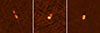 |
Fig. 1. VLASS images at |

We explored the properties of the compact sources in more detail and show in Fig. 2 the distribution of rmaj.. Most of them are apparently unresolved sources, with  , but a tail of marginally resolved sources is also present. The distribution of deconvolved sizes has a median of
  , corresponding to ∼8 kpc at the median redshift of the sample.
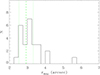 |
Fig. 2. Distribution of the length of the major axis, rmaj., obtained from a two-dimensional Gaussian fit on the VLASS images of the 29 HzRQs. The dashed vertical line marks the median value of rmaj. of the VLASS sources in the same range of declination, and the two dotted lines mark the observed spread of |

3. The radio spectra
For the 29 selected QSOs, we gathered radio data at different frequencies. The GLEAM EGC provided us with 20 measurements from 76 to 227 MHz, which we complemented with the flux densities at 1.4 GHz from the Faint Images of the Radio Sky at Twenty centimeters survey, (FIRST; Becker et al. 1995; Helfand et al. 2015) and the National Radio Astronomy Observatory Very Large Array Sky Survey (NVSS; Condon et al. 1998), at 3 GHz from the VLASS, and the 5 GHz from the Green Bank 6 cm survey (GB6; Gregory et al. 1996). The cross-match for the NVSS and GB6 was performed by adopting a search radius of 15″ from the location of the VLASS source, while a search radius of 3″ was used for FIRST.
Three examples of the resulting radio spectra are presented in Fig. 3, and all radio spectra are presented in the appendix.
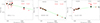 |
Fig. 3. Three examples of radio spectra. The low-frequency regime is covered by the GLEAM data (small red circles). Because the errors are relatively large, we also provide flux densities by rebinning five frequency channels (large black circles). The other flux densities are taken from the NVSS (black squares), FIRST (red squares), VLASS (red triangles), and GB6 (black triangles). Only data with a similar spatial resolution (i.e., from GLEAM, NVSS, and GB6, all marked with black symbols) are used to obtain the linear fit, which is represented by the green line. |
The radio spectra are generally well represented by a single power law in the form Fν ∝ ν−α over the whole frequency range. We derived the radio spectrum index α with a weighted linear fit in logarithmic units. For the fit, we considered only the radio flux density measurements obtained at similar spatial resolution (i.e., from GLEAM, NVSS, and GB6). The high-resolution data from FIRST and VLASS are shown in the radio spectra to verify their consistency with the low-resolution data, but were excluded because these surveys might be missing extended structures. The spectral indices are listed in Table 1, and their distribution is shown in Fig. 4. The highest measured value of the spectral index is α = 0.87, and therefore, we did not find any ultrasteep radio sources associated with HzRQs, which agrees with the results of Sotnikova et al. (2021).
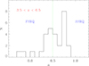 |
Fig. 4. Distribution of spectral indices for the QSO with 3.5 < z < 6.5. The vertical dashed green line separates flat- from steep-spectrum sources, that is, FSRQs from SSRQs. |
By using α = 0.5 as a threshold to separate flat from steep spectra, we find following the definition of Condon (1984) that 15 QSOs (45%) have flat radio spectra. All of them are unresolved sources at the VLASS spatial resolution. Several of these FSRQs show a relatively large scatter from the power-law fit; for example, SDSS 144516.46+095836.0 shown in the right panel of Fig. 3. This is likely to be due to variability in their radio emission, as expected from objects that are amplified by Doppler boosting. None of the FSRQs shows clear evidence of a steepening radio spectrum at low frequencies, as would be expected in case of a significant contribution from diffuse, steep spectrum emission. There is a marginal increase in the fraction of flat sources, fFSRQ, within this redshift range: The redshift of the eight FSRQs among the 14 objects (57%) is higher than the median value. However, a test of equal proportions (Wilson 1927) indicates that this difference is not statistically significant.
From the fit to the radio spectra, we estimated the luminosity of the 29 QSOs at a fixed rest-frame frequency of 500 MHz, P500. We find that P500 ranges from ∼0.7 × 1028 W Hz−1 to ∼40 × 1028 W Hz−1, with a median of ∼4.6 × 1028 W Hz−1.
4. Biases in the sample selection
The selection of the sample at low frequency introduces a bias as it might miss sources with a turnover at low frequency: This is the case of the compact steep-spectrum sources (CSS), which are thought to be young radio sources, in which the low-frequency emission is depressed due to self-absorption, for example (see O’Dea & Saikia 2021 for a review of the properties of CSS).
We investigated this issue in more detail and included the quasars with z > 3.5 and δ < 30° in the EGC area. We selected the QSOs with a detection in FIRST. CSS at high redshift are expected to be unresolved in the FIRST images (the spatial resolution of FIRST at z ∼ 3.5 is ∼35 kpc), and we do not expect that they miss radio flux from extended structures. We estimated their radio power at the rest-frame frequency of 5 GHz, P5000, (above the typical turnover frequency of CSS) and considered those with L5000 > 4 × 1027 W Hz−1, the minimum luminosity at this frequency of the selected sample of 29 quasars extracted from the EGC in the previous section. We then derived their radio spectra by including the flux densities from TGSS, FIRST, VLASS, and GB6. We find that a large fraction of them (38 out of 54) has a flat spectrum, which is inconsistent with a CSS identification. Other sources have a steep spectrum and are detected by the TGSS, but their flux density is lower than the EGC threshold: These are correctly not included in our sample. The remaining 8 sources are likely CSS, with a steep spectrum between FIRST and VLASS and a nondetection (or a turnover) based on the TGSS. The CSS fraction derived from this analysis (∼20%) agrees with the results of Coppejans et al. (2017). In Fig. 5 we show the radio spectrum of one such source, in which the flux density upper limit from the TGSS lies below the measured value at 1.4 GHz. The inclusion of these (intrinsically) steep sources in the sample might reduce fFSRQ to 35%.
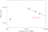 |
Fig. 5. Example of a source with a turnover at low frequency, a likely CSS, missed by our selection at low frequency. The solid line is the best line fit to the high-frequency data. The extrapolation of the fit at low frequency (dotted line) is higher by a factor > 10 than the upper limit from the TGSS. |
5. Selection and analysis of the lower-redshift samples
In order to set our results in a broader context, we selected three further samples of quasars at lower redshift, namely at 1.2 < z < 1.4, 2.0 < z < 2.1, and 2.7 < z < 2.8. These three redshift bins were selected to uniformly cover the range from the well-studied radio source samples (up to z ∼ 1) to the high-redshift sources (z > 3.5). The bin sizes were chosen to include a sufficient number of sources for a robust statistical analysis. The selection method was the same as we used for the highest-redshift QSO, that is, a cross-match between SDSS QSO and GLEAM sources followed by the verification of the radio-optical association with the VLASS images. However, for these samples, we only chose QSOs with a radio power P500 > 1028 W Hz−1 for consistency with the luminosity range of the HzRQ sample. The total number of sources in the various redshift bins is 50 for 1.2 < z < 1.4, 42 for 2.0 < z < 2.1, and 39 for 2.7 < z < 2.8.
We estimated their radio spectral indices. The distributions at the different redshifts are compared in Fig. 6. There is a marked difference in these distributions. Sources with a higher redshift have flatter spectra in general. More quantitatively, in the top panel of Fig. 7, we show the evolution of the fraction of FSRQs (i.e., sources with α < 0.5). It increases with redshift from ∼8% at z ∼ 1.3 to ∼45% at z > 3.5 (see Table 2 for a summary of the results).
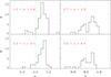 |
Fig. 6. Distribution of spectral indices for powerful radio quasars (L500 > 1028 W Hz−1) in the four redshift bins considered (the bottom panel reproduces the same distribution as in Fig. 4 for the z > 3.5 QSOs). The vertical dashed green line separates flat- from steep- spectrum sources. The fraction of FSRQS increases at increasing redshift. |
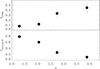 |
Fig. 7. Evolution of the fraction of FSRQ, fFSRQ (top), and of the fraction of extended radio sources (bottom) with redshift. The uncertainties are estimated by adopting the Poisson statistic. |
Results obtained for the various QSO samples considered.
Following the same strategy as adopted in Sect. 4, we searched for candidate CSS in these lower-redshift samples. We found 4, 5, and 4 such sources at 1.2 < z < 1.4, 2.0 < z < 2.1, and 2.7 < z < 2.8, respectively. The corresponding CSS fractions are similar (ranging from 7% to 10%) and smaller than we found for the highest-redshift sources (∼20%). However, the small number statistics prevents us from drawing any strong conclusion about the evolution of the CSS fraction with redshift.
The fraction of extended sources instead decreases with redshift, from ∼80% to ∼15%. This latter effect is not due to the different redshift ranges of the sources considered because with the adopted cosmological parameters, the scale varies from 7.4 kpc arcsec−1 at z = 3.5 to 8.5 kpc arcsec−1 at z = 1.3. In both cases, a sharp transition appears to occur at z ∼ 2.5. The sizes of the radio sources also show a strong evolution with redshift (see Fig. 8): While in the lowest redshift bin we considered, the size of about half of the QSOs exceeds ∼100 kpc, no QSO with z > 3.5 is associated with such a large radio source.
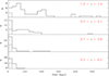 |
Fig. 8. Evolution of the distribution of the deconvolved sizes of the radio sources, fextended with redshift. The dashed area of the histograms represents the upper limits to the size of the unresolved sources. |
6. Exploring the properties of quasars with a lower radio luminosity
The selection of sources detected in the GLEAM observations sets a lower limit to the radio luminosity of the quasars considered of P500 ≳ 1028 W Hz−1. These sources, to which we refer as the bright sample, then represent the extreme high-power end of the population of radio quasars. We here explore the properties of quasars with a lower radio luminosity to test whether the results obtained above apply more generally to the overall population and to set them on a stronger statistical basis.
The selection was again performed at low frequency, but using the images produced by data release 2 of LOFAR LoTSS, which covers ∼5700 square degrees. The advantage of using LoTSS data is that their depth exceeds that of the GLEAM images (the LoTSS reaches a ∼80% completeness at 0.8 mJy), at the expense of losing the information on the full low-frequency radio spectrum. However, having established that a power law provides a good representation of the radio spectra of HzRQs, we can rely on the LOFAR data, combined with higher-frequency measurements, to separate SSRQs from FSRQs.
We selected the quasars with z > 3.5 that were covered by both LoTSS and FIRST. We adopted a threshold for the flux density at 150 MHz of 5 mJy. With this restriction, we can set a lower limit on their spectral index between 150 MHz and 1.4 GHz for all quasars that were not detected by FIRST α150, 1400 ≳ 0.7, and they can be safely classified as SSRQ. We selected 172 quasars, to which we refer to as the faint sample, 21 of which do not have a FIRST counterpart to the LOFAR source. At this stage, we also included the VLASS flux density measurements. By assuming that their radio spectra are reproduced with a single power law, as seen in the high-power sources, we estimated the spectral slopes with a weighted linear fit in log-log space including measurements from LOFAR, FIRST, and VLASS. The distribution of spectral indices we obtained is shown in Fig. 9. The fraction of FSRQ obtained with this method is 47%, which is similar to that found for the bright sample.
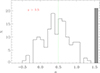 |
Fig. 9. Distribution of the spectral indices obtained with a linear fit to the LOFAR, FIRST, and VLASS data to the sources of the faint sample, that is, with P500 ≳ 1027 W Hz−1. The gray bar represents the 21 sources that were not detected by in the high-frequency surveys. The vertical dashed green line separates FSRQs from SSRQs. |
Following the same strategy as adopted in the previous section, we also explored the behavior of quasars at lower redshift by estimating their radio spectral slopes. We limited the analysis to sources within the same luminosity range as for the higher redshift bin, that is, P500 > 1027 W Hz−1. The results are summarized in Table 2. The evolution of fFSRQ with redshift is similar to that observed in the bright sample, although the fraction of FSRQs appears to decrease less sharply with redshift.
7. Discussion
7.1. Evolution of radio spectral indices and the fraction of obscured RLAGN
The main result of our analysis is the strong increase in the fraction of FSRQ, fFSRQ, with redshift. FSRQs are radio sources in which the highly relativistic jets form a small angle with the line of sight, and their emission is amplified by the effects of Doppler boosting. The fraction of FSRQs within a population of radio sources can be estimated as fFSRQ ∼ 1/(2Γ2), where Γ is the jet bulk Lorentz factor. We consider as highly boosted sources all those seen at an angle θ ≲ 1/Γ. This is a reasonable assumption considering the strong dependence of the Doppler boosting factor on the viewing angle. By reversing this argument, it is possible to estimate the number of sources expected to be the misaligned counterparts (i.e., HzRGs and SSRQs) of a given sample FSRQ.
However, for a flux-limited sample, or for sources that were selected based on the observed radio luminosity, this line of reasoning does not hold, as already pointed out by Lister et al. (2019). This is because FSRQs might exceed the threshold of the sample only because of the contribution of the nuclear beamed emission. Their isotropic radio emission, which is mainly produced by the extended structures, might instead be significantly lower than those of the SSRQs selected at the same flux density (or luminosity) threshold. Considering the steepness of the luminosity function of radio-loud AGN, a flux-limited sample includes a large number of FSRQs with a lower isotropic luminosity that that of the SSRQs.
We then followed a different approach and considered samples of radio quasars that covered the same range of radio luminosity at different redshifts. When we assume that the beaming factor and the slope of the luminosity function do not change with redshift, the fraction of FSRQs within the population of radio sources (including both narrow- and broad-line object) above a given observed luminosity are not expected to vary. The observed increase in fFSRQ with redshift within the quasar population is due to a corresponding decrease in the fraction of SSRQs.
For the most powerful quasars, we find fFSRQ ∼ 8% for z ∼ 1.2 and fFSRQ ∼ 45% for z > 3.5. When we consider the likely CSS sources (as discussed in Sects. 3.1 and 4), this fraction might be reduced to fFSRQ ∼ 13/(29 + 8)∼35% in the high-redshift sample and to fFSRQ ∼ 7% in the lowest redshift bin.
When we consider the whole population of RLAGN at low redshift, they split almost equally into obscured and unobscured sources. The fraction of beamed objects is significantly smaller, ∼1/(2Γ2). As a result of Doppler boosting, however, this fraction increases in a flux luminosity-limited sample to the observed value of ∼8% of the QSOs at z ∼ 1.3. These FSRQs are sources of lower isotropic radio luminosity that meet the selection due the amplification of their nuclear emission. Under the assumptions (i) that the beaming factor and the slope of the luminosity function at high luminosities do not change with redshift and (ii) that a purely orientation AGN unified model is valid, the fraction of FSRQs with respect to the whole population of RLAGN is expected to be constant. This is because in the scenario we assumed, the beamed sources are drawn from the same range of isotropic luminosity and are boosted by the same factor. At high redshift, the fraction of obscured sources is not known because only the unobscured sources (the QSOs) are visible. However, the observed increase in fFSRQ to ∼45% at z > 3.5, which is a factor ∼5 higher than at z ∼ 1.3 (and the same effect is obtained by considering the presence of CSS in both samples), can be explained when the fraction of SSRQs decreases by the same amount, that is, from ∼50% to ∼10%. The remaining 90% of the RLAGN population are obscured in the optical band and appear as high-redshift radio galaxies.
A similar conclusion was reached by Ghisellini & Sbarrato (2016). They suggested that at z > 4, jetted sources are almost completely surrounded by obscuring material in order to account for the relatively low number of radio sources that can represent the misaligned parent population from which FSRQs are drawn. (Caccianiga et al. 2024) found no evidence for obscuration in RLAGN within angles of ∼10° −20° from the jet axis through modeling of their luminosity function. This is not in contrast with our results. Several studies (see, e.g., Merloni et al. 2014; Vijarnwannaluk et al. 2022) suggested that most high-redshift AGN are obscured. The large fraction of obscured sources at high-z we derive from our study also extends this conclusion to the population of radio loud AGN.
7.2. Evolution of the size of the radio sources
Another difference between the lower- and higher-redshift radio quasars is the fraction of extended sources, which drops from 80% at z = 1.2 to ∼15% for z > 3.5 with a strong decrease with the redshift of the sizes of the extended sources. We tested whether this can be explained as an orientation effect. The fraction of SSRQs statistically corresponds to a maximum viewing angle with respect to our line of sight of ∼25°. The foreshortening expected for this range of orientations causes the angular size of a source to be reduced by an average factor of ∼3.
At low redshift, the maximum viewing angle instead is ∼50°, corresponding to an average foreshortening by a factor 1.8, which is only 1.4 times smaller than at higher redshift. We conclude that the smaller angular size of the radio sources that is associated with high-redshift quasars with respect to those at lower redshift is mainly due to an intrinsic effect. We argue that this is due to the same dense gas that causes the obscuration of their nuclei, which lows the expansion of the radio source. This idea is reminiscent of the early suggestion that compact steep-spectrum sources are those in which the progress of their jets is hampered by the large amount of gas in their nuclear regions (e.g., van Breugel et al. 1984).
This interpretation suggests that the CSS fraction should increase with redshift. This is indeed observed, as this fraction increases from 7%−10% for z ∼ 1.3 − 2.8 and reaches ∼20% at the highest redshift probed by our analysis. However, the small number statistics prevents us from drawing any strong conclusion about the evolution of the CSS fraction with redshift.
7.3. Are there ultrasteep sources among the HzRQs?
Another interesting result is that we found no USS among the highest-redshift powerful radio quasars, that is, sources with a radio spectrum with a slope α > 1, even though the selection of low frequencies should favor the inclusion of sources like this. Conversely, the faint sample contains 12 quasars with α > 1 out of a total of 91 SSRQ, which corresponds to 13%. This fraction can be higher (up to 36%) due to the large number of sources (21) for which the nondetection in FIRST and VLASS does not enable us to estimate their spectral slope.
We stress this result because, as reported in the Introduction, most HzRGs (the parent population of radio quasars) were found by obtaining spectra of the optical counterparts of ultrasteep radio sources. The broad-band radio spectra we obtained for the SSRQ indicate that USS are instead quite rare even at z > 3.5. The lower observed spectral slopes with respect to those required for a USS classification cannot be due to the contribution of a bright flat radio core. The signature of this effect is a spectrum with a high α value at low frequencies, followed by a sharp flattening at higher frequencies where the core emission becomes dominant. This is not observed in any of the high-z SSRQs.
This result implies that although this method is very efficient (the fraction of USS that are indeed at high redshift is quite high; see, e.g., Röttgering et al. 1997), it misses the bulk of the RLAGN population. Furthermore, the HzRGs selected with this procedure might be biased and may not represent the overall population.
8. Summary and conclusions
We explored the radio properties of a sample of 29 high-redshift (z > 3.5) SDSS quasars selected at low frequency (76 MHz) based on GLEAM observations. The selected sources are all very powerful radio AGN, with a rest-frame luminosity at 500 MHz L500 MHz ≳ 1028 W Hz−1. We complemented the GLEAM data with those of other radio surveys at higher frequencies, namely NVSS, FIRST, VLASS, and GB6, and we obtained radio spectra ranging from 76 MHz to 5 GHz. The spectra are generally well reproduced with a single power law with a range of slopes between α ∼ −0.3 to α ∼ 0.9 (defined as fν ∝ ν−α). The sample contains a large fraction (∼45%) of flat-spectrum sources, that is, with α < 0.5.
The selection at low frequency is instrumental for building a sample in which the radio emission is dominated by the large-scale optically thin emission to reduce the orientation effects. However, this choice biases the sample against the inclusion of radio sources with a turnover at low frequency, that is, of the CSS. We estimate that nine CSS at z > 3.5 with the same power at high frequency as the main sample are excluded from the selection.
We studied the evolution of the QSOs by comparing the properties of samples with a lower redshift. Again at low frequency, we selected radio quasars with a threshold of the radio power L500 ≳ 1028 W Hz−1. We find that the fraction of FSRQs increases with redshift from 8% at z = 1.2 to ∼45% at z > 3.5, with a sharp upturn at z ≳ 2.5. A similar result is found by studying quasar samples that were selected from the deeper low-frequency survey LoTSS, which extended the range of radio power down to L500 ∼ 1027 W Hz−1. We interpret this effect as due to a corresponding decrease in the fraction of steep-spectrum quasars that becomes as low as ∼10% at high redshift. Under the assumptions (i) that the beaming factor and the slope of the luminosity function do not change with redshift and (ii) that a purely orientation AGN unified model is valid, this implies that the central regions in ∼90% of the powerful radio-loud AGN at high redshift cannot be observed because they are obscured in the optical and UV bands. They can only be recognized as quasars when their are seen within a rather small angle, ∼25°, from our line of sight. This supports previous suggestions that the bulk of the high-redshift AGN population is enshrouded by a large amount of gas and dust.
The radio structures of high-redshift quasars are also much more often compact (with a typical size of ∼8 kpc) than those of quasars of similar power at lower redshift. We also found a trend for the size of radio sources to decrease with increasing redshift. This change cannot simply be due to a projection effect, which only plays a marginal role (we estimate that the average foreshortening for the high-redshift sources is only 1.4 higher than at low redshift), but it is likely due to the very same dense gas that surrounds the more distant sources, which slows the source expansion down.
We conclude that most high-redshift radio-loud AGN do not manifest themselves as quasars, but as radio galaxies. This population is still poorly studied because it is difficult to identify these objects. As discussed in Sect. 1, the typical targets of spectroscopic studies that searched for HzRGs are the ultrasteep radio sources. In this study, we did not find any bright QSO with a steep radio spectrum, and the faint sample contained only a small fraction. Under the assumption that the radio spectra of SSRQs are representative, as suggested by the RLAGN unifying model also of their misaligned counterparts (i.e., of HzRGs), the general population of HzRGs currently remains largely elusive.
Available at https://cirada.ca/vlasscatalogueql0
References
- Antonucci, R. 1993, ARA&A, 31, 473 [Google Scholar]
- Antonucci, R. R. J. 1982, Nature, 299, 605 [NASA ADS] [CrossRef] [Google Scholar]
- Antonucci, R. R. J. 1984, ApJ, 278, 499 [NASA ADS] [CrossRef] [Google Scholar]
- Baldi, R. D., Capetti, A., Buttiglione, S., Chiaberge, M., & Celotti, A. 2013, A&A, 560, A81 [NASA ADS] [CrossRef] [EDP Sciences] [Google Scholar]
- Barthel, P. D. 1989, ApJ, 336, 606 [Google Scholar]
- Becker, R. H., White, R. L., & Helfand, D. J. 1995, ApJ, 450, 559 [Google Scholar]
- Bennett, C. L., Larson, D., Weiland, J. L., & Hinshaw, G. 2014, ApJ, 794, 135 [Google Scholar]
- Best, P. N., Kauffmann, G., Heckman, T. M., et al. 2005, MNRAS, 362, 25 [Google Scholar]
- Caccianiga, A., Moretti, A., Belladitta, S., et al. 2019, MNRAS, 484, 204 [NASA ADS] [CrossRef] [Google Scholar]
- Caccianiga, A., Ighina, L., Moretti, A., et al. 2024, A&A, 684, A98 [NASA ADS] [CrossRef] [EDP Sciences] [Google Scholar]
- Condon, J. J. 1984, ApJ, 287, 461 [Google Scholar]
- Condon, J. J., Cotton, W. D., Greisen, E. W., et al. 1998, AJ, 115, 1693 [Google Scholar]
- Coppejans, R., van Velzen, S., Intema, H. T., et al. 2017, MNRAS, 467, 2039 [NASA ADS] [Google Scholar]
- Croton, D. J., Springel, V., White, S. D. M., et al. 2006, MNRAS, 365, 11 [Google Scholar]
- De Breuck, C., van Breugel, W., Röttgering, H., et al. 2001, AJ, 121, 1241 [NASA ADS] [CrossRef] [Google Scholar]
- De Breuck, C., Klamer, I., Johnston, H., et al. 2006, MNRAS, 366, 58 [NASA ADS] [CrossRef] [Google Scholar]
- Fabian, A. C. 2012, ARA&A, 50, 455 [Google Scholar]
- Fanaroff, B. L., & Riley, J. M. 1974, MNRAS, 167, 31P [Google Scholar]
- Ghisellini, G., & Sbarrato, T. 2016, MNRAS, 461, L21 [NASA ADS] [CrossRef] [Google Scholar]
- Gloudemans, A. J., Duncan, K. J., Röttgering, H. J. A., et al. 2021, A&A, 656, A137 [NASA ADS] [CrossRef] [EDP Sciences] [Google Scholar]
- Gloudemans, A. J., Saxena, A., Intema, H., et al. 2023, A&A, 678, A128 [NASA ADS] [CrossRef] [EDP Sciences] [Google Scholar]
- Gregory, P. C., Scott, W. K., Douglas, K., & Condon, J. J. 1996, ApJS, 103, 427 [NASA ADS] [CrossRef] [Google Scholar]
- Gürkan, G., Hardcastle, M. J., Best, P. N., et al. 2019, A&A, 622, A11 [NASA ADS] [CrossRef] [EDP Sciences] [Google Scholar]
- Helfand, D. J., White, R. L., & Becker, R. H. 2015, ApJ, 801, 26 [NASA ADS] [CrossRef] [Google Scholar]
- Hill, G. J., Goodrich, R. W., & Depoy, D. L. 1996, ApJ, 462, 163 [NASA ADS] [CrossRef] [Google Scholar]
- Hurley-Walker, N., Callingham, J. R., Hancock, P. J., et al. 2017, MNRAS, 464, 1146 [Google Scholar]
- Intema, H. T., Jagannathan, P., Mooley, K. P., & Frail, D. A. 2017, A&A, 598, A78 [NASA ADS] [CrossRef] [EDP Sciences] [Google Scholar]
- Ivezić, Ž., Menou, K., Knapp, G. R., et al. 2002, AJ, 124, 2364 [CrossRef] [Google Scholar]
- Jiang, L., Fan, X., Ivezić, Ž., et al. 2007, ApJ, 656, 680 [Google Scholar]
- Kellermann, K. I., Sramek, R., Schmidt, M., Shaffer, D. B., & Green, R. 1989, AJ, 98, 1195 [Google Scholar]
- Krezinger, M., Perger, K., Gabányi, K. É., et al. 2022, ApJS, 260, 49 [NASA ADS] [CrossRef] [Google Scholar]
- Lacy, M., Baum, S. A., Chandler, C. J., et al. 2020, PASP, 132, 035001 [Google Scholar]
- Lawrence, A. 1991, MNRAS, 252, 586 [NASA ADS] [Google Scholar]
- Lister, M. L., Homan, D. C., Hovatta, T., et al. 2019, ApJ, 874, 43 [NASA ADS] [CrossRef] [Google Scholar]
- Lyke, B. W., Higley, A. N., McLane, J. N., et al. 2020, ApJS, 250, 8 [NASA ADS] [CrossRef] [Google Scholar]
- Merloni, A., Bongiorno, A., Brusa, M., et al. 2014, MNRAS, 437, 3550 [Google Scholar]
- Miley, G., & De Breuck, C. 2008, A&ARv, 15, 67 [Google Scholar]
- Miley, G., & Chambers, K. 1989, Eur. South. Obs. Conf. Workshop Proc., 32, 43 [NASA ADS] [Google Scholar]
- Miraghaei, H., & Best, P. N. 2017, MNRAS, 466, 4346 [NASA ADS] [Google Scholar]
- O’Dea, C. P., & Saikia, D. J. 2021, A&ARv, 29, 3 [Google Scholar]
- Röttgering, H. J. A., van Ojik, R., Miley, G. K., et al. 1997, A&A, 326, 505 [Google Scholar]
- Saxena, A., Marinello, M., Overzier, R. A., et al. 2018, MNRAS, 480, 2733 [Google Scholar]
- Shen, Y., Richards, G. T., Strauss, M. A., et al. 2011, ApJS, 194, 45 [Google Scholar]
- Shimwell, T. W., Hardcastle, M. J., Tasse, C., et al. 2022, A&A, 659, A1 [NASA ADS] [CrossRef] [EDP Sciences] [Google Scholar]
- Sotnikova, Y., Mikhailov, A., Mufakharov, T., et al. 2021, MNRAS, 508, 2798 [CrossRef] [Google Scholar]
- Spinrad, H., Marr, J., Aguilar, L., & Djorgovski, S. 1985, PASP, 97, 932 [CrossRef] [Google Scholar]
- Swarup, G. 1991, ASP Conf. Ser., 19, 376 [Google Scholar]
- Tadhunter, C. 2016, A&ARv, 24, 10 [Google Scholar]
- Tadhunter, C. N., Morganti, R., Robinson, A., et al. 1998, MNRAS, 298, 1035 [NASA ADS] [CrossRef] [Google Scholar]
- Tingay, S. J., Goeke, R., Bowman, J. D., et al. 2013, PASA, 30, e007 [Google Scholar]
- Urry, C. M., & Padovani, P. 1995, PASP, 107, 803 [NASA ADS] [CrossRef] [Google Scholar]
- van Breugel, W., Miley, G., & Heckman, T. 1984, AJ, 89, 5 [Google Scholar]
- van Haarlem, M. P., Wise, M. W., Gunst, A. W., et al. 2013, A&A, 556, A2 [NASA ADS] [CrossRef] [EDP Sciences] [Google Scholar]
- Vijarnwannaluk, B., Akiyama, M., Schramm, M., et al. 2022, ApJ, 941, 97 [NASA ADS] [CrossRef] [Google Scholar]
- Voit, G. M., Donahue, M., Bryan, G. L., & McDonald, M. 2015, Nature, 519, 203 [NASA ADS] [CrossRef] [Google Scholar]
- Volonteri, M., Haardt, F., Ghisellini, G., & Della Ceca, R. 2011, MNRAS, 416, 216 [Google Scholar]
- Wayth, R. B., Lenc, E., Bell, M. E., et al. 2015, PASA, 32, e025 [Google Scholar]
- Willott, C. J., Rawlings, S., Blundell, K. M., & Lacy, M. 2000, MNRAS, 316, 449 [NASA ADS] [CrossRef] [Google Scholar]
- Wilson, E. B. 1927, J. Am. Stat. Assoc., 22, 209 [CrossRef] [Google Scholar]
- Yamashita, T., Nagao, T., Ikeda, H., et al. 2020, AJ, 160, 60 [NASA ADS] [CrossRef] [Google Scholar]
- York, D. G., Adelman, J., Anderson, J. E., et al. 2000, AJ, 120, 1579 [Google Scholar]
Appendix A: Radio spectra of the 29 high-redshift quasars
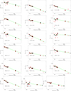 |
Fig. A.1. Radio spectra of the 29 quasars with z > 3.5. Considering the relatively large errors of the GLEAM data (small red circles) we provide flux densities by rebinning five frequency channels (large black circles). The other flux densities are from the NVSS (black squares), FIRST (red squares), VLASS (red triangles), and GB6 (black triangles). |
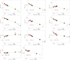 |
Fig. A.1. continued. |
All Tables
All Figures
|
Fig. 1. VLASS images at |
| In the text | |
|
Fig. 2. Distribution of the length of the major axis, rmaj., obtained from a two-dimensional Gaussian fit on the VLASS images of the 29 HzRQs. The dashed vertical line marks the median value of rmaj. of the VLASS sources in the same range of declination, and the two dotted lines mark the observed spread of |
| In the text | |
|
Fig. 3. Three examples of radio spectra. The low-frequency regime is covered by the GLEAM data (small red circles). Because the errors are relatively large, we also provide flux densities by rebinning five frequency channels (large black circles). The other flux densities are taken from the NVSS (black squares), FIRST (red squares), VLASS (red triangles), and GB6 (black triangles). Only data with a similar spatial resolution (i.e., from GLEAM, NVSS, and GB6, all marked with black symbols) are used to obtain the linear fit, which is represented by the green line. |
| In the text | |
|
Fig. 4. Distribution of spectral indices for the QSO with 3.5 < z < 6.5. The vertical dashed green line separates flat- from steep-spectrum sources, that is, FSRQs from SSRQs. |
| In the text | |
|
Fig. 5. Example of a source with a turnover at low frequency, a likely CSS, missed by our selection at low frequency. The solid line is the best line fit to the high-frequency data. The extrapolation of the fit at low frequency (dotted line) is higher by a factor > 10 than the upper limit from the TGSS. |
| In the text | |
|
Fig. 6. Distribution of spectral indices for powerful radio quasars (L500 > 1028 W Hz−1) in the four redshift bins considered (the bottom panel reproduces the same distribution as in Fig. 4 for the z > 3.5 QSOs). The vertical dashed green line separates flat- from steep- spectrum sources. The fraction of FSRQS increases at increasing redshift. |
| In the text | |
|
Fig. 7. Evolution of the fraction of FSRQ, fFSRQ (top), and of the fraction of extended radio sources (bottom) with redshift. The uncertainties are estimated by adopting the Poisson statistic. |
| In the text | |
|
Fig. 8. Evolution of the distribution of the deconvolved sizes of the radio sources, fextended with redshift. The dashed area of the histograms represents the upper limits to the size of the unresolved sources. |
| In the text | |
|
Fig. 9. Distribution of the spectral indices obtained with a linear fit to the LOFAR, FIRST, and VLASS data to the sources of the faint sample, that is, with P500 ≳ 1027 W Hz−1. The gray bar represents the 21 sources that were not detected by in the high-frequency surveys. The vertical dashed green line separates FSRQs from SSRQs. |
| In the text | |
|
Fig. A.1. Radio spectra of the 29 quasars with z > 3.5. Considering the relatively large errors of the GLEAM data (small red circles) we provide flux densities by rebinning five frequency channels (large black circles). The other flux densities are from the NVSS (black squares), FIRST (red squares), VLASS (red triangles), and GB6 (black triangles). |
| In the text | |
|
Fig. A.1. continued. |
| In the text | |
Current usage metrics show cumulative count of Article Views (full-text article views including HTML views, PDF and ePub downloads, according to the available data) and Abstracts Views on Vision4Press platform.
Data correspond to usage on the plateform after 2015. The current usage metrics is available 48-96 hours after online publication and is updated daily on week days.
Initial download of the metrics may take a while.