| Issue |
A&A
Volume 689, September 2024
|
|
|---|---|---|
| Article Number | A67 | |
| Number of page(s) | 12 | |
| Section | Extragalactic astronomy | |
| DOI | https://doi.org/10.1051/0004-6361/202449642 | |
| Published online | 02 September 2024 | |
Molecular gas excitation in the circumgalactic medium of MACS1931–26
1
ESO, Karl Schwarzschild Strasse 2, 85748 Garching, Germany
2
Department of Physics & Astronomy, University of British Columbia, 6224 Agricultural Road, Vancouver, BC V6T 1Z1, Canada
3
School of Astronomy and Space Science, Nanjing University, Nanjing, China
4
Key Laboratory of Modern Astronomy and Astrophysics, Nanjing University, Ministry of Education, Nanjing, China
5
Fukui University of Technology, 3-6-1, Gakuen, Fukui City, Fukui Pref. 910-8505, Japan
6
Research Center for Astronomical Computing, Zhejiang Laboratory, Hangzhou 311100, China
7
Aix Marseille Univ., CNRS, CNES, LAM, 13388 Marseille, France
Received:
17
February
2024
Accepted:
11
June
2024
Abstract
The evolution of galaxies is largely affected by exchanging material with their close environment, the circumgalactic medium (CGM). In this work, we investigate the CGM and the interstellar medium (ISM) of the bright central galaxy (BCG) of the galaxy cluster, MACS1931−26 at z ∼ 0.35. We detected [CI](2−1), 12CO(1−0), and 12CO(7−6) emission lines with the APEX 12-m and NRO 45-m telescopes. We complemented these single-dish observations with 12CO(1−0), 12CO(3−2), and 12CO(4−3) ALMA interferometric data and inferred the cold molecular hydrogen physical properties. Using a modified large velocity gradient (LVG) model, we modelled the CO and CI emission of the CGM and BCG to extract the gas thermodynamical properties, including the kinetic temperature, the density, and the virialisation factor. Our study shows that the gas in the BCG is highly excited, comparable to the gas in local ultra luminous infrared galaxies (ULIRGs), while the CGM is likely less excited, colder, less dense, and less bound compared to the ISM of the BCG. The molecular hydrogen mass of the whole system derived using [CI](2−1) is larger than the mass derived from 12CO(1−0) in literature, showing that part of the gas in this system is CO-poor. Additional spatially resolved CI observations in both transitions, [CI](1−0) and [CI](2−1), and the completion of the CO SLED with higher CO transitions are crucial to trace the different phases of the gas in such systems and constrain their properties.
Key words: galaxies: clusters: general / galaxies: evolution / submillimeter: galaxies
Corresponding author; This email address is being protected from spambots. You need JavaScript enabled to view it. .
© The Authors 2024
 Open Access article, published by EDP Sciences, under the terms of the Creative Commons Attribution License (https://creativecommons.org/licenses/by/4.0), which permits unrestricted use, distribution, and reproduction in any medium, provided the original work is properly cited.
This article is published in open access under the Subscribe to Open model. This email address is being protected from spambots. You need JavaScript enabled to view it. to support open access publication.
1. Introduction
In the past decades, advances in observing techniques and galaxy formation simulations drew attention to the role of the circumgalactic medium (CGM) as a key ingredient to understand how material is exchanged between galaxies and their cosmological environment (Werk et al. 2014; Tumlinson et al. 2017; Nelson et al. 2020). The CGM is defined as the multiphase gaseous halo extending from the outermost part of the galactic disc to the virial radius of the dark matter halo (Tumlinson et al. 2017). For reference, the virial radius of a Milky-Way galaxy type is estimated to be ∼200 kpc (Shull 2014). Due to the diffuse nature of its gas, the exact extent of CGM is not straightforward to measure. However, observations of Neutral Hydrogen (HI) in z < 1 massive galaxies hint a CGM extent of ∼350 kpc (Wilde et al. 2021). Inflows from the CGM to galaxies provide metal-poor gas as a fuel for galactic growth and sustaining star formation (Voit 2021; Donahue & Voit 2022; Faucher-Giguère & Oh 2023). Such inflows are predicted by galaxy formation models (Lochhaas et al. 2020; Esmerian et al. 2021), however, they are difficult to be detected due to their extended spatial structure and faint emission. On the other hand, outflows powered by active galactic nuclei (AGNs) and star formation deposit metals back into the CGM (Cheung et al. 2016; Prochaska et al. 2017; Christensen et al. 2018). These outflows can escape the potential well of their host galaxy or “rain back” onto the galaxies depending on their energy (Voit 2021). They can be detected more easily closer to their launch regions compared to when they arrive at the CGM because they are more compact at their launch regions. The physical conditions of the CGM could provide clues about potential inflows and outflows between a galaxy and its CGM (Voit et al. 2017).
The CGM could be observed using both absorption and emission line spectroscopy. The warm and hot phase of CGM (T > 104 K) could be detected in absorption against bright background quasars mostly in optical and ultraviolet using neutral hydrogen and ionised lines of heavier elements (Tumlinson et al. 2011, 2017; Donahue & Voit 2022; Koplitz et al. 2023). Ultraviolet surveys such as COS-Halos (Tumlinson et al. 2013; Werk et al. 2016), the Keck baryonic structure survey (KBSS; Rudie et al. 2012, 2019), and the cosmic ultraviolet baryon survey (CUBS; Chen et al. 2020; Zahedy et al. 2021; Qu et al. 2022) provide a rich sample of absorption line studies of the CGM of galaxies up to z ∼ 2. Although this method is sensitive to a wide range of densities, it only provides information about one line of sight towards the CGM and the background quasar.
The Ly-α transition of neutral hydrogen is the strongest emission from CGM (Erb et al. 2023). This extended emission has been observed using the multi-unit spectroscopic explorer (MUSE) at the ESO-very large telescope (VLT) recently (Wisotzki et al. 2016, 2018; Chen et al. 2021). Despite the weak emission of H2 due to the lack of a permanent dipole moment, observing CGM and intergalactic medium (IGM) molecular gas is possible using the mid-infrared rotational H2 lines which trace the warm molecular gas (T ∼ 100 K) partially (15%−30%; Togi & Smith 2016; Appleton et al. 2017, 2023).
The cold phase of H2 (T ∼ 10 K–20 K; Faucher-Giguère & Oh 2023) is usually traced using other species, including CO and CI. CO is the second most abundant molecule after H2 and is a reliable proxy for molecular hydrogen in the local universe (Bolatto et al. 2013). However, CO might fail in tracing all the H2 content in some cases due to the dependence on redshift, radiation field, metallicity, gas excitation, and the cosmic rays (CR) ionisation rate (Bisbas et al. 2017; Valentino et al. 2018; Madden et al. 2020). Specifically, CRs might be one of the main heating sources of gas in and around star-forming galaxies since CRs can penetrate deeply into molecular clouds and regulate the thermal balance of the gas (Papadopoulos 2010; Grenier et al. 2015; Gaches et al. 2019; Bisbas et al. 2021). CRs can destroy CO in molecular clouds and leave large swathes of CO-poor/([CI]–[CII])-rich gas (Bisbas et al. 2015, 2017; Papadopoulos et al. 2018). In these cases, a combination of CO and CI is a good tracer of the cold molecular gas content of the CGM.
Interferometers provide high-resolution observations of CGM that are crucial to study the structure and kinematics of this gas. However, interferometers cannot detect the emission of scales larger than their largest angular scale which is determined by the shortest baseline of the observing configuration (Plunkett et al. 2023). Hence, due to the diffuse and extended (∼200 kpc) nature of CGM, it is not straightforward for interferometers to detect the whole extent of CGM. Single-dish observation, on the other hand, are able to detect the emission of scales as large as their field of view (Lee et al. 2024). Combining the information obtained from both single-dish and interferometric observations is thus necessary to study the CGM.
On the observational front, recent studies have been able to detect CGM, IGM, and intracluster medium (ICM) using the CO and CI emission lines originating from cold gas. These streams seem to feed the star formation activity of galaxies as a part of the baryon cycle in the CGM. For instance, multiphase emission from the tidal streams in the IGM of a galaxy group, Stephan’s Quintet, is detected at z = 0.02 (Appleton et al. 2023). Extended molecular structures are found in halos (r ∼ 10 − 20 kpc) of z ∼ 2.2 QSO (Scholtz et al. 2023) and out to r ∼ 200 kpc (Cicone et al. 2021). Emonts et al. (2023) find a [CI](1−0) stream around the massive z = 3.8 radio galaxy 4C 41.17, likely linked to its strong star formation. CO and [CI](1−0) molecular winds are imaged in local luminous infrared galaxies (LIRGs; Cicone et al. 2018). These winds seem to be linked to AGN and star formation at a rate of SFR ∼ 20−140 M⊙ yr−1 (Cicone et al. 2014). Stronger molecular outflows originating from galaxies in clusters with SFR ∼ 150−250 M⊙ yr−1 can eject gas and dust further away from the CGM into the intracluster medium (Fogarty et al. 2019; Emonts et al. 2018).
Extracting information about the physical conditions of the gas detected in the spectral lines of different species, requires both radiative transfer modelling and assumptions about the excitation of the gas (van der Tak et al. 2007; Roueff et al. 2024). The fastest and simplest framework for this problem is the local thermodynamic equilibrium (LTE) assumption which holds in high densities and states that the excitation temperature equals the kinetic temperature. However, this assumption might introduce biases to the line excitation modelling (Roueff et al. 2021). Some non-LTE methods, including the large velocity gradient assumption (LVG; Sobolev 1960), consider a local excitation, meaning that the species excitation is a result of their interactions with local radiation field. For instance, RADEX (van der Tak et al. 2007) is a non-LTE code, solving the radiative transfer and molecular excitation under the LVG assumption which is widely used in molecular excitation studies. More sophisticated radiative transfer methods can treat the problem in a non-local way (Asensio Ramos & Elitzur 2018). However, these models are computationally expensive and more complicated to implement (Roueff et al. 2024).
In this work, we trace the molecular gas content of the BCG of a galaxy cluster, MACS1931−26 (hereafter MACS1931), and its CGM using a combination of CO and CI emission lines. Our goal is to model the thermodynamical state of the gas in CGM and BCG using a radiative transfer code and study the potential differences of gas in these two components of the galaxy. The MACS1931 galaxy cluster is an excellent testbed for investigating the physical conditions of molecular gas in the ISM inside the BCG and its CGM due to its strong star formation activity and X-ray-loud AGN (SFR ∼ 250 M⊙ yr−1; Ehlert et al. 2011; Santos et al. 2016; Fogarty et al. 2017, 2019). MACS1931 is a cool-core galaxy cluster having one of the largest known H2 reservoirs (∼2 × 10¹⁰ M⊙) in a cluster core revealed by the Atacama Large Millimeter/submillimeter Array (ALMA) 12CO(3−2) and 12CO(1−0) imaging (Fogarty et al. 2019; Rose et al. 2019). An appreciable fraction of this mass is found over a tail-like structure extending up to 30 kpc from the BCG core (Fogarty et al. 2019). This tail-like structure (hereafter tail) is a part of the multiphase CGM of the central galaxy and contains a large reservoir of Tdust ∼ 10 K dust.
Similar to the Phoenix cluster BCG (Russell et al. 2017), the BCG of MACS1931 and its tail-like structure have a low gas-to-dust ratio of ∼10 − 25 (Fogarty et al. 2019) lower than the Galactic value of 100 − 150 (Draine & Lee 1984; Rémy-Ruyer et al. 2014). The unusually low ratio suggests that a potentially large H2 gas reservoir might have been missed by the existing CO observations, perhaps due to the CR-irradiation rendering some of the H2 gas CO-poor, and/or because ALMA long baseline interferometric observations might have filtered out extended 12CO(1−0) line emission (Lee et al. 2024). To investigate this matter further, we obtained additional single-dish 12CO(1−0) observations to be able to recover the total flux, which might be filtered out in interferometric observations, along with high-frequency CO and CI observations in order to probe the gas physical conditions. While the detected CO emission with ALMA represents only part of the whole CGM1 of MACS1931 BCG, observations with existing single-dish telescopes can help determine how much of the emission is over-resolved by ALMA. The detection of CO and CI emission at 30 kpc from MACS1931 offers a unique opportunity to study a cloud that is likely part of the CGM surrounding this BCG.
In this article, we report new 12CO(1−0), 12CO(7−6), and [CI](2−1) single-dish observations towards the MACS1931 galaxy cluster at z = 0.3525. We complement these data with the ALMA/ACA observations presented in Fogarty et al. (2019) and use the combined dataset to provide an analysis of the average physical conditions of the BCG and its CGM in this galaxy cluster. Throughout, we adopt a Λ-CDM Cosmology as defined by Planck Collaboration XIII (2016) where H0 = 67.8 km s−1 Mpc−1 and Ωm = 0.308.
2. The observations
In this section, we report the methods and details of the observations of the [CI](2−1), 12CO(1−0), and 12CO(7−6) lines with the APEX 12-m and the NRO 45-m antenna telescopes as well as the archival ALMA data towards MACS1931, used to complement our single-dish data.
2.1. APEX observations
We used the Atacama Pathfinder EXperiment (APEX) telescope (Güsten et al. 2006) equipped with the SEPIA660 receiver (Belitsky et al. 2018) tuned at the frequencies of the 12CO(7−6) and [CI](2−1) lines (central frequency of 609.5 GHz). The observations of MACS1931−26 for this project were obtained from 2021 June 25 to 2023 April 27 (project ID: E-0106.A-0997A-2020, PI: P. Andreani). The data taken in April 2023 did not meet good quality standards and were omitted from the analysis.
The APEX/SEPIA660 receiver is a single-pixel heterodyne receiver working at the frequency window of 597−725 GHz. The total integration time was 20 hours, centring towards the BCG on the direction of  Dec = −26° 34′34″. The precipitable water vapour (PWV) was 0.4−0.9 mm on June 25, 0.2−0.8 mm on June 28, and 0.1−0.4 mm on June 29. The intended spectral lines, [CI](2−1) with a rest frequency of 809.34 GHz and 12CO(7−6) with a rest frequency of 806.65 GHz, are redshifted to the frequencies of 598.40 GHz and 596.41 GHz at the redshift of z = 0.3525 (Fogarty et al. 2019), respectively. The wobbler mode used in these observations had an amplitude of 50″ and a frequency of 1.5 Hz. The half-power beam width (HPBW) of APEX for this observation is 9.89″ ± 0.11″.
We reduced the data using the GILDAS/CLASS2 (Pety et al. 2005) software package. Two parts of the APEX spectrum near 595 GHz (O3) and 600 GHz (O3 + HDO) are affected by atmospheric absorption (Pardo et al. 2022). For each scan, we excluded ∼0.3 GHz of the spectrum at the frequency of each atmospheric line. A first-order baseline was then fitted to each scan and subtracted from the spectrum. Finally, we averaged the spectra of all scans and fitted Gaussian functions for the 12CO(7−6) and [CI](2−1) emission lines. The RMS noise of this spectrum is 0.66 mK per channel with channel width of 82 km s−1, measured using CLASS on continuum-free line-free channels. No planet was available during the observations. Instead, calibration observations were performed on the source IRAS15194−5115. These reference spectra were compared to the calibration observations on the same source in performed in mid 2022. The flux ratio of this calibrator source was applied to cross scans of Mars obtained in 2022 June with SEPIA660, yielding the antenna gain of3Γ = (72 ± 8) Jy/K for 2021 which we used to convert the observed brightness temperature to flux density.
After data reduction within GILDAS/CLASS, we performed a Monte Carlo simulation using the Astropy and Specutils Python packages (Astropy Collaboration 2022; Earl et al. 2023) to estimate the uncertainty of these measurements. In each realisation, we added an artificial Gaussian error to the data with a standard deviation equal to the RMS of the data (47 mJy per channel). Then, we fitted Gaussian functions to both lines and measured all of the line properties in each realisation. The reported values in Table 1 are the median and standard deviation of these parameters.
Line flux and luminosity towards MACS1931.
2.2. NRO 45-m dish observations
The 12CO(1−0) single-dish observations towards MACS1931 were taken with the 45-m telescope of the Nobeyama radio observatory (NRO) in Japan, which is equipped with the FOur-beam REceiver front-end (FOREST; Minamidani et al. 2016). FOREST is a four-beam (2 × 2) dual-polarization sideband-separating SIS mixer receiver for the single sideband (SSB) operation. 12CO(1−0) has a rest frequency of 115.27 GHz that is redshifted to 85.22 GHz at z = 0.3525. The frequency coverage and the resolution for each array are set to 1 GHz and 244.14 kHz, respectively, giving a velocity coverage and resolution of ∼3500 km s−1 and 0.86 km s−1 at 85.22 GHz. At this frequency, the HPBW of the 45-m telescope with FOREST is ∼18″. We adopted the ON-ON observation mode, which uses two of the four beams of the FOREST receiver at the diagonal (beams 1 and 3). Since the two beams are separated by 70″ in the sky, one of the beams observes the object while another the sky when the apparent size of the object is smaller than the beams. The dominant observation overhead is therefore the slewing time for beam switching. We adopted a switching period of 10 s cycle to optimize the observation overhead and the bandpass stability (Nakajima et al. 2013).
The data were taken on 2022 March 1, 2, and 12. The observing time for each day was roughly 5 hours, while the on-source time was 3.8, 6.4, and 5.8 hours (total hours for beam 1 and beam 2, and H- and V-polarisation). The system temperature was 255 K, 247 K and 211 K for each day, respectively. In order to check the absolute pointing accuracy, we observed a point source (GL2370), which is the closest and strongest SiO maser source to the target using a 43 GHz band receiver every hour. The reported antenna temperature was obtained by the chopper wheel method, yielding the  scale, which contains corrections for atmospheric and any antenna Ohmic losses as well for beam pattern rearward spillover and losses (Kutner & Ulich 1981). The main beam brightness temperature, Tmb was converted from
  , for each intermediate frequency by observing a standard source, the carbon star IRC+10216. The scaling factors take into account the main-beam efficiency (ηmb) of the 45-m antenna, but also compensate for the decrease in line intensity due to the imperfect SSB image rejection.
The reduction of the NRO 45-m data towards MACS1931 was carried out using the NEWSTAR software (Ikeda et al. 2001) which is a data reduction package designed for this telescope. After flagging out the bad spectra, we integrated the spectra for each schedule. A first-order baseline was then subtracted from the spectra and the intensities were corrected with a point-source Jy/K conversion factor of Γ = (6.54 ± 0.33) Jy/K. Finally, we integrated the spectra over all schedules and smoothed the resulted spectrum to a velocity channel of bin width 50 km s−1. We derived an aperture efficiency of ηA ∼ 0.28 ± 0.06, appropriate for the observed frequency and elevation from the information provided by the observatory4. The source declination allowed us to conduct observations at elevations ∼30° above the horizon. The source was detected in each observing run, however, it was heavily affected by the atmospheric absorption with an RMS noise of 2.6 mJy per 50 km s−1 channel. The line properties and uncertainties were calculated using the same method as the APEX data (Table 1).
2.3. Archival ALMA data
We used archival ALMA data towards MACS1931 published by Fogarty et al. (2019) to complement our single-dish data. The observations were obtained in ALMA Band 3, cycle 4 (Project ID: 2016.1.00784.S, PI: M. Postman) and Band 6 and 7, cycle 5 (Project ID: 2017.1.01205.S, PI: M. Postman). The Band 3 data is a combination of two ALMA 12-m array configurations with a total integration time of 13 366 s, minimum synthesised beam of 0.54″ and maximum recoverable scale of 18.8″. The Band 6 data towards MACS1931 is a combination of an ALMA 12-m array configuration with 726 s integration time and an Atacama compact array (ACA) configuration with an integration time of 1724 s. The minimum synthesised beam and maximum recoverable scale are 0.74″ and 20.4″, respectively. Finally, the Band 7 data is a combination of the 12-m array (integration time of 2722 s) and ACA (integration time of 6804 s), yielding minimum synthesised beam and maximum recoverable scale are 0.81″ and 14.6″, respectively (Fogarty et al. 2019). We used the CO line measurements of Fogarty et al. (2019) to complement our data and model the gas excitation.
3. Results
In this section, we present and analyse the results of the APEX and NRO 45-m observations of MACS1931 combined with the archival ALMA data. These single-dish observations do not have the required spatial resolution to distinguish between the BCG and the tail of MACS1931 and we use the ALMA observations of Fogarty et al. (2019) as a prior to understand the molecular gas geometry and kinematics. However, we are able to detect the tail emission spectrally using the [CI](2−1) line with APEX.
We present the detected CO and CI lines in Figure 1. The upper left panel shows 12CO(1−0) spectrum obtained with NRO 45-m/FOREST receiver. The upper right panel shows the [CI](2−1) and 12CO(7−6) spectrum obtained with the APEX/SEPIA660 receiver. Despite the atmospheric noise affecting the APEX high-frequency data and the NRO 45-m low elevation data of MACS1931, the lines are detected, albeit at low statistical significance. To extract the line properties over an integrated region as large as the HPBW (∼10″ and ∼18″ for APEX and NRO 45-m, respectively), we used a Lorentzian fitting function as well as a Gaussian function. We employed the Lorentzian fits because in the following we compare the fluxes extracted from these single-dish observations with those reported by Fogarty et al. (2019) using a Lorentzian fitting function. As described in Fogarty et al. (2019), the spectrum of each line has a bimodal distribution including a larger peak corresponding to the BCG and a more redshifted smaller peak corresponding to the tail. Because of the low S/N in single-dish observations, this bimodal distribution is only detectable in the [CI](2−1) spectrum (Figure 1). As a reference for the line properties, we used the second velocity component (C2) of 12CO(3 − 2) reported in Fogarty et al. (2019) corresponding to the 30 kpc tail-like structure since this line has the highest S/N in their work. Assuming that the velocity offset between the two peaks and the FWHM of the small peak are the same as the 12CO(3 − 2) line from Fogarty et al. (2019), we extracted the line properties, including line widths, fluxes, and luminosities, reported in Table 1.
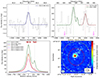 |
Fig. 1. Submillimeter observations towards MACS1931. Upper left: Gaussian fit to the 12CO(1−0) line in the NRO 45-m observations of MACS1931. The black histogram shows the spectrum. The blue solid curve shows the Gaussian fit to the line. Upper right: Gaussian fit to the [CI](2−1) and 12CO(7−6) lines in the APEX observations of MACS1931. The black histogram shows the spectrum. The green and red solid curves show the Gaussian fits to the [CI](2−1) and 12CO(7−6) lines, respectively. The magenta solid lines show the regions of the spectrum excluded because of the atmospheric lines. Lower left: Best-fit line profiles of 12CO(1−0), 12CO(3−2), and 12CO(4−3) from Fogarty et al. (2019) (dashed curves) and Lorentzian fits on 12CO(1−0), 12CO(7−6), and [CI](2−1) from this work (solid curves) displayed on the same plot for comparison (see Sect. 3 and Table 1). The CGM tail peak of the 12CO(4−3) line from Fogarty et al. (2019) is the best fit to a partially truncated spectrum due to a spectral window gap in the ALMA Band 7 observations. Lower right: The ALMA 12CO(3−2) intensity map of the MACS1931 BCG and the tail. The moment zero map is calculated over a range of [ − 500, 600] km s−1. ALMA beam is shown by an ellipse on the bottom left side of the image. The APEX and NRO 45-m HPBWs are shown by solid red and dashed yellow circles. Contours are calculated on the moment map with levels [0.2, 0.5, 1, 2]σ and σ = 0.297 Jy beam−1 km s−1. The CGM tail component of the spectra is detectable in the [CI](2−1) line as well as all lines from Fogarty et al. (2019). |
The best-fit parameters of these models are listed in Table 1 together with uncertainties resulting from the calibration, data reduction, and error estimation process described in the previous section. The lower right panel of Figure 1 shows a comparison between the beam sizes of ALMA, APEX, and NRO 45-m observations. Based on this figure, the tail is distributed from the BCG (the centre of the field of view) up to ∼6″ away from the centre. Hence, a fraction of the tail flux is not captured by the APEX and NRO 45-m telescopes due to the beam response. A Gaussian beam response function was assumed to calculate the “beam corrected” fluxes and luminosities in Table 1. The exact extent of the tail-like CGM component is not measurable and the emission is not spatially resolved in these single-dish observations. Therefore, in order to account for the Gaussian beam response, we assumed the tail to be a point source at a distance of ∼4″ from BCG and the beam centre and increased the tail flux by a fraction for the beam response correction. Considering that the APEX HPBW is 9.89″, the tail flux drops by ∼40% at the distance of 4″ in a Gaussian beam. So, we added this fraction to the tail flux of [CI](2−1) measured before. We also added this fraction to the upper limit flux of 12CO(7−6) measured from APEX data. Through a similar analysis for NRO 45-m dish with a HPBW of 18″, we added ∼15% to our upper limit estimation of the tail flux in 12CO(1−0).
From the spectra of the 12CO(7−6) and 12CO(1−0) lines, we determined the line flux of the BCG and extract upper limits on the tail flux values. We report the 3σ upper limits for these lines (see Table 1) by computing  , where RMS is the noise per channel of the spectrum, Nchan = 2FWHMCO(3 − 2)/δv is the number of line channels, and δv is the channel width (82 km s−1 and 50 km s−1 for APEX and NRO 45-m, respectively). The lower left panel of Figure 1 shows the Lorentzian line models for all the CI and CO lines detected for MACS1931 reported in this work and Fogarty et al. (2019) for comparison. The line luminosity ratios, in units of L′ [K km s−1 pc2], inferred for MACS1931 for all the reported lines for the BCG and tail components are listed in Table 2. Line luminosities are computed following (Solomon et al. 1997):
 (1)
(1)
Line luminosity ratios towards MACS1931−26.
where SlineΔV is the integrated line flux; νobs is the redshifted frequency; DL is the luminosity distance; and z is the redshift of the object.
Figure 1 shows that the [CI](2−1) line is brighter than the 12CO(7−6) line and the full width at half maximum (FWHM) is similar for both lines within the error bars. This is indicative of a highly excited warm gas rich in atomic Carbon. The single-dish flux value of the 12CO(1−0) line (2.5 ± 0.6 Jy km s−1 using a Lorentzian fit) is in agreement with the one detected with ALMA 12-m array reported in Fogarty et al. (2019) (3.02 ± 0.42 Jy km s−1) within the error bars. It would imply that the ALMA interferometric observations do not filter out flux from an extended component of this system. Notice that the maximum recoverable angular scale in Band 3 for the observations reported by Fogarty et al. (2019) is 18.8″ is almost equal to the half-power beam width of the NRO 45-m observations (see Sect. 2). Consequently, missing 12CO(1−0) flux in ALMA observations is not the main reason for the low gas-to-dust ratio of MACS1931. We investigate further whether this system contains some CO-poor gas seen using different tracers.
3.1. Spectral line energy distribution and profiles
The new observations reported in this work help to further constrain the physical state of the gas content of this system. Figure 2 shows the normalised CO flux ratios against the rotational quantum number, the so-called CO spectral line energy distribution (CO SLED), of the BCG and tail separately. The line luminosities are normalised to the interferometric 12CO(1−0) line values obtained by from Fogarty et al. (2019) for both BCG and tail. In the CO SLED of the tail, we do not display the 12CO(7−6)/12CO(1−0) ratio because we only have an upper limit of the 12CO(7−6) flux that is not stringent enough to constrain the CO SLED. In Figure 2, the CO SLED of MACS1931 is compared to those of local ULIRGs (Papadopoulos et al. 2012a), submillimetre galaxies (Bothwell et al. 2013), BzK galaxies (Daddi et al. 2015), quasars (Molyneux et al. 2023) and local IR galaxies observed by Herschel (Kamenetzky et al. 2016). The line flux ratios of the MACS1931 BCG are particularly large similar to those found in local ULIRGs (Papadopoulos et al. 2012a; Montoya-Arroyave et al., in prep.). These large values are characteristics of high excitation, likely ascribed to starburst gas. On the contrary, the line flux ratios related to the tail component of MACS1931 do not show the same trend as the BCG, implying that the excitation of CO in the tail is different from that in the BCG and in ULIRGs. Moreover, the 12CO(4−3)/12CO(3−2) ratio is relatively low which differs from that measured in Milky Way-like galaxies (Figure 2; Kamenetzky et al. 2016). It is noteworthy that the ALMA Band 7 spectrum of MACS1931 is truncated around the relative velocity of 300 − 500 km s−1 for the 12CO(4−3) line, and the reported line flux in Fogarty et al. (2019) is based on the best fitted Lorentzian function on this partially obscured spectrum. Hence, the actual 12CO(4−3) flux might be different from the reported value. More observations of different CO lines, especially higher transitions like 12CO(5−4), would be beneficial to better constrain the CO SLED of the tail. We put models into practice to interpret these results.
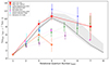 |
Fig. 2. CO SLED built with the available data for the BCG and the CGM tail of MACS1931 (red and orange stars, respectively). The CO line fluxes are taken from Fogarty et al. (2019), except 12CO(7−6) of the BCG which is detected in this work using APEX. Line fluxes are normalised to the 12CO(1−0) flux taken from Fogarty et al. (2019). Additional average CO SLEDs from the literature are added for comparison: ULIRGs from Papadopoulos et al. (2012a, blue circles), SMGs from Bothwell et al. (2013, green circles), BzK galaxies from Daddi et al. (2015, purple circles), low-redshift Herschel galaxies from Kamenetzky et al. (2016, magenta circles), and quasars from the QFeedS sample published in Molyneux et al. (2023, cyan circles). The dashed black line shows the theoretical CO SLED for resolved objects with ΣSFR = 0.83 M⊙ yr−1 kpc−2 modelled by Narayanan & Krumholz (2014). This value is the estimated ΣSFR for the MACS1931 BCG (Fogarty et al. 2015). The grey shaded area shows the predicted CO SLED range with this model for 0.6 < ΣSFR [M⊙ yr−1 kpc−2] < 3. We report an upper limit on the 12CO(7−6) flux for the tail in Table 2, however, it is not constraining the tail CO SLED and falls out of the range of this plot. |
3.2. Line ratio modelling
The inference of the physical state of gas from the molecular line luminosities is not straightforward. We can constrain the gas thermodynamical properties using the observed line fluxes with the help of reasonable physical assumptions. To this aim, we used a non-local thermodynamic equilibrium (non-LTE) radiative transfer code, i.e. MyRadex5 (Du 2022) to map the [nH2, Tkin, Kvir] parameter space for the CO lines. This parameter space includes the molecular hydrogen number density (nH2), kinetic temperature (Tkin), and the virialisation parameter Kvir = (dV/dR)/(dV/dR)vir which is a measure of the virialisation of the gas based on its velocity gradient. MyRadex is a revised version of RADEX (van der Tak et al. 2007), that fits the CO SLED with a large velocity gradient (LVG) model and adds as an additional constraint the CI flux value (Papadopoulos et al. 2018). It solves the statistical equilibrium problem with the LSODE6 solver in ODEPACK7 and avoids unconverged solutions under some parameters compared to the original RADEX. We used the CO and CI molecular data from the Leiden atomic and molecular database (LAMDA8; Schöier et al. 2005) and assumed background temperature as the cosmic microwave background (CMB) temperature at the cluster redshift, Tback(z) = TCMB(z) = 3.69 K.
We made a grid of numbers in the [nH2, Tkin, Kvir] parameter space, composed of ![Mathematical equation: $ 0.7 < {\log{\frac{T_{\mathrm{kin}}}{\mathrm{[K]}}}} < 3 $](/articles/aa/full_html/2024/09/aa49642-24/aa49642-24-eq7.gif) with an increment of 0.11 dex,
with an increment of 0.11 dex, ![Mathematical equation: $ 1 < {\log{\frac{n_{\mathrm{H_2}}}{\mathrm{[cm^{-3}]}}}} < 7 $](/articles/aa/full_html/2024/09/aa49642-24/aa49642-24-eq8.gif) with an increment of 0.1 dex, and 1 < Kvir < 100 with an increment of 0.1 dex. Then, we fitted a model for each point in our parameter space using MyRadex, and calculated the likelihood of each model based on the observations of CO and CI, following the method of Papadopoulos et al. (2014). The probability for each observation follows a Gaussian distribution, using P = exp(−χ2/2), while χ2 = Σi(1/σi)2[Robs(i) − Rmodel(i)]2, where Robs is the ratio of the measured line luminosities, σi the error of the measured line ratio, and Rmodel the ratio of the line brightness temperatures calculated by the LVG model. We used the [CI](2−1) observation as the additional constraint in our model. In particular, we used the ratio [CI](2−1)/12CO(1−0) instead of the atomic Carbon ratio, [CI](2−1)/[CI](1−0), due to lack of the [CI](1−0) line observation.
with an increment of 0.1 dex, and 1 < Kvir < 100 with an increment of 0.1 dex. Then, we fitted a model for each point in our parameter space using MyRadex, and calculated the likelihood of each model based on the observations of CO and CI, following the method of Papadopoulos et al. (2014). The probability for each observation follows a Gaussian distribution, using P = exp(−χ2/2), while χ2 = Σi(1/σi)2[Robs(i) − Rmodel(i)]2, where Robs is the ratio of the measured line luminosities, σi the error of the measured line ratio, and Rmodel the ratio of the line brightness temperatures calculated by the LVG model. We used the [CI](2−1) observation as the additional constraint in our model. In particular, we used the ratio [CI](2−1)/12CO(1−0) instead of the atomic Carbon ratio, [CI](2−1)/[CI](1−0), due to lack of the [CI](1−0) line observation.
Using the definition of the line luminosity from Equation (1) and optically thin assumption, we can derive the [CI](2−1) luminosity following Papadopoulos et al. (2004) and Lei et al. (2023) as
 (2)
(2)
where mH2 is the mass of a single H2 molecule; μ = 1.36 corrects for the mass in He; C is the conversion between pc2 and cm2; A21 = 2.68 × 10⁻⁷ s−1 is [CI](2−1) spontaneous emission coefficient (Einstein coefficient); XC = [C]/[H2] = 3 × 10⁻⁵ is the Carbon abundance (Papadopoulos et al. 2022); c is light speed; k is the Boltzmann constant; h is the Planck constant; ν0 is [CI](2−1) rest frequency; and Q21 = N2/NCI < 1 is the CI excitation factor depends on (nH2, Tkin) derived using equations from Papadopoulos et al. (2004). Using the LVG assumption, Papadopoulos et al. (2012b) derived CO conversion factor  as
as
 (3)
(3)
where α = 1.5 for typical cloud density profile, Tb, 1 − 0 is 12CO(1−0) brightness temperature, derived using LVG code depend on (nH2, Tkin, Kvir). Thus, we can derive  and add this as an additional constraint to the χ2 calculations.
Figures 3 and 4 show the best-fitted models for the BCG and the tail, respectively. The top panels of both figures show the distribution of the models in the Tkin, nH2 space where the colours show the [CI](2−1)/12CO(1−0) ratio of the model that has the highest likelihood between models with the same Tkin, nH2, but different Kvir. Black contours show the levels of [CI](2−1)/12CO(1−0) and white contours show the likelihood levels. The white star represents the best-fitted solution based on observations. The bottom panels of both Figures 3 and 4 show the CO SLED of the models compared to observations. The black curve represents the best-fitted model with the highest likelihood. The blue points show the CO line observations. The green curves show the scatter of the best models after applying the Markov chain Monte Carlo (MCMC) sampling to the solutions. We set wide parameter range in the MCMC sampling by assuming flat priors for ![Mathematical equation: $ 5 < {\frac{T_{\mathrm{kin}}}{\mathrm{[K]}}} < 10^3 $](/articles/aa/full_html/2024/09/aa49642-24/aa49642-24-eq13.gif) ,
, ![Mathematical equation: $ 1 < {\log{\frac{n_{\mathrm{H_2}}}{\mathrm{[cm^{-3}]}}}} < 7 $](/articles/aa/full_html/2024/09/aa49642-24/aa49642-24-eq14.gif) , 1 < Kvir < 100 in logarithmic scale with prior probability P(p) = 1, and set P(p) = 0 for solutions outside the prior criteria (Papadopoulos et al. 2014). The best models predict the gas properties of
, 1 < Kvir < 100 in logarithmic scale with prior probability P(p) = 1, and set P(p) = 0 for solutions outside the prior criteria (Papadopoulos et al. 2014). The best models predict the gas properties of  K,
K, ![Mathematical equation: $ \mathrm{\log{\frac{n_{\mathrm{H_2}}}{\mathrm{[cm^{-3}]}}}}=4.5_{-0.8}^{+1.3} $](/articles/aa/full_html/2024/09/aa49642-24/aa49642-24-eq16.gif) , and
, and  for BCG and
  K,
K, ![Mathematical equation: $ {\log{\frac{n_{\mathrm{H_2}}}{\mathrm{[cm^{-3}]}}}}=3.5_{-1.6}^{+2.2} $](/articles/aa/full_html/2024/09/aa49642-24/aa49642-24-eq19.gif) , and
, and  for tail. Based on the current data and models, we argue that the tail gas might be cooler, less dense, and less bound compared to the BCG gas, on average. Considering that the CR energy density in a star-forming galaxy with strong AGN activity is expected to be higher than the CR energy density in Milky-Way, kinetic temperatures below ∼20 K for the tail gas are difficult to explain theoretically (see Figure 2 of Papadopoulos et al. 2011). It is noteworthy that the top panel of Figure 3 shows two possible solutions for the BCG (white contours), one colder and denser and one hotter and more diffuse with lower probability. However, a temperature of more than 1000 K is not physical for the BCG gas. Thus, we do not consider the second solution as a valid model. This degeneracy in the [nH2 − Tkin] space is inherent to this kind of models and can only be broken with additional independent observations, as the ratio of the two atomic carbon lines, [CI](1−0)/[CI](2−1) and a better sampling of the CO ladder. Figure A.1 presents the joint distribution of the model parameters for all MCMC samplings. These plots show that the physical conditions of the BCG are better constrained compared to the CGM tail. Moreover, the model predictions for the physical conditions of these two galaxy components are sufficiently separate by 2σ in the nH2 − Tkin plane. However, Kvir is not well constrained for any of the galaxy components.
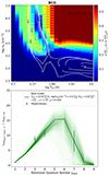 |
Fig. 3. Top: LVG modelling for the BCG of MACS1931. The Tkin, nH2 grid is plotted with a projected Kvir axis. At each point of the Tkin, nH2 grid, the colour shows the predicted [CI](2−1)/12CO(1−0) ratio of the model with the highest likelihood among models with different Kvir values. The black contours show the levels of the modelled [CI](2−1)/12CO(1−0) flux ratio which is shown by colours. The white contours show the likelihood levels. The white star indicates the best-fitted LVG model obtained from MCMC simulations. Bottom: The CO SLED of the best-fitted LVG model for BCG. The black curve shows the modelled CO SLED. The blue points with blue error bars show the observed line flux ratios. The green curves show the distribution of best models obtained from MCMC. |
4. Discussion
4.1. CGM tail formation and excitation
Our models in Section 3.2 show that the BCG of MACS1931 has the kinetic temperature of  K, the molecular hydrogen number density of
 ![Mathematical equation: $ {\log{\frac{n_{\mathrm{H_2}}}{\mathrm{[cm^{-3}]}}}}=4.5_{-0.8}^{+1.3} $](/articles/aa/full_html/2024/09/aa49642-24/aa49642-24-eq22.gif) , and the virialistion parameter of
, and the virialistion parameter of  . The modelled kinetic temperature of the detected gas in BCG is less than the dust temperature of 33 K, estimated by Santos et al. (2016) using the Herschel photometry, but because of the large error bars we may conclude that the two temperatures are similar and the BCG gas is thermalised.
In the MACS1931 CGM tail, we detect gas with a low kinetic temperature,  K, a molecular hydrogen number density of
 ![Mathematical equation: $ {\log{\frac{n_{\mathrm{H_2}}}{\mathrm{[cm^{-3}]}}}}=3.5_{-1.6}^{+2.2} $](/articles/aa/full_html/2024/09/aa49642-24/aa49642-24-eq25.gif) , and a virialistion parameter of
, and a virialistion parameter of  . In this case, one could conclude that Tkin > Tdust ∼ 10 K (Fogarty et al. 2019) and the gas might not be in LTE conditions (Papadopoulos et al. 2022) with the [CI](2−1) gas in a subthermal state. However, in addition to the large uncertainties of the Tkin measurements, the value of Tdust estimated by Fogarty et al. (2019) is also affected by the uncertainties related to the dust model and the subsequent value assumed for the dust emissivity index.
For the CGM tail of MACS1931, the high 12CO(3−2)/12CO(1−0) brightness temperature ratio ( , Table 2) is consistent with both cold and dense as well as warmer (and less dense) molecular gas in the known number density-kinetic temperature (ne − Tkin) degeneracy. This is inherent in the radiative transfer modelling of optically thick lines like those of CO. However, this high brightness temperature ratio is typically associated with the warm ISM found in starbursts. Indeed the observed 12CO(3−2)/12CO(1−0) ratio (R31) in the CGM tail is identical to the mean value found for the star-forming ISM of Luminous Infrared Galaxies (LIRGs) (see Figure 5 in Papadopoulos et al. 2012a). In their study, additional 12CO(1−0) and 13CO line observations limit the
  degeneracy in the LIRGs studied, attributing such high 12CO(3−2)/12CO(1−0) ratios to the warm end of the ne − Tkin parameter space. Figure 4 shows that the predicted CO SLED of the tail models can peak at different Jupper values. But because of the large error bars on the existing data and the lack of higher-Jupper CO transitions the CGM gas status cannot be pinned down consequently.
The BCG and CGM of MACS1931 contain warm molecular hydrogen, observed in the preliminary data analysis of a cycle 2 MIRI/MRS program with JWST (program ID: 3629, PI: A. Man). Mapping and modelling the JWST warm hydrogen data and the ALMA cold hydrogen data in this system will shed new light on the multiphase nature of the CGM gas and provide clues on the role of the CRs in the excitation of CGM and it is the subject of a following paper. Confirming a warm H2 gas phase concomitant with such a cold dust using additional molecular, atomic line, and dust continuum observations, would verify the thermal decoupling of the two phases of the gas, and the role of CRs in warming the gas (but not the dust) rather than the usual star formation-originating far ultraviolet (FUV) radiation fields. In particular, the R31 ratio seems to be sensitive to an enhanced CR energy density (Bisbas et al. 2023). Here we must mention that in principle turbulence can also warm the gas but not the dust in terms of the global energy budget necessary. However, the detailed picture emerging from simulations as well as observations is that only a small fraction (∼1 − 2%) of a supersonically turbulent gas reservoir is heated to extraordinarily high temperatures (∼1500−2000 K) while the bulk remains very cold (∼10−15 K; Wu et al. 2017; Bisbas et al. 2021).
Fogarty et al. (2019) shows that the tail direction is not aligned with the AGN jet axis. They argue that this tail-like structure is likely an infalling feature which has been ejected out of the galaxy by AGN jets in an outburst long ago. This structure is currently falling back into the galaxy and fueling the active star formation of MACS1931 BCG due to a more recent AGN outburst which uplifted the gas and now the gas is condensed and raining back to the galaxy. Ciocan et al. (2021) studies the ionised and molecular gas phases of MACS1931 using VLT-MUSE optical integral field spectroscopy and archival ALMA observations. They show that both CO and Hα emission are co-spatial and share similar kinematics. This study highlights that the gas phase metallicity measured form optical lines in the CGM tail is more than that in the BCG. Their findings are in agreement with the scenario suggested by Fogarty et al. (2019). Ehlert et al. (2011) finds two bright ridges about 25−30 kpc to the north and south direction of the BCG using Chandra X-ray observations. This study probes gas with a temperature of 107 − 108 K and a density of 10−3 − 10−1 cm−3. The northern ridge, which is co-spatial with the CGM component as seen in the ALMA observations, is the coldest (kBT = 4.78 ± 0.64 keV), densest (ρ ∼ 0.09 cm−3), and the most metal-rich (Z = 0.53 ± 0.11 Z⊙) region in the cluster. They argue that these ridges originally formed as a result of a previous cluster merger and an AGN outburst in the BCG. Furthermore, Subaru optical observations presented in Ehlert et al. (2011) show continuum emission from a young stellar population in both north and south of the BCG and Hα emission from star-forming regions only in the north of BCG, almost coinciding with the north X-ray ridge. They suggest that the metal-rich cool core of the cluster has been stripped and moved to the north of the BCG as a result of a previous cluster merger. The tail-like structure detected in ALMA observations lies approximately in the northern X-ray ridge and the star-forming region detected in optical. Our results show that the molecular gas in the tail is colder than the molecular gas in the BCG, consistent with the condensation scenario. However, we need more information to understand whether the dynamical state of cluster post-merger affects the star formation of the BCG.
4.2. Molecular hydrogen mass inferred from [CI](2–1)
An estimate of the molecular hydrogen mass in MACS1931 can be obtained by rearranging Equation (2) as
![Mathematical equation: $$ \begin{aligned} M_{\rm H_2} [M_{\odot }] = 1375.8 \frac{D_{\rm L}^{2}}{1+z} \left(\frac{X_{\rm CI}}{10^{-5}}\right)^{-1} \left(\frac{A_{21}}{10^{-7}}\right)^{-1} Q_{21}^{-1} \frac{{S\!}_{\rm [{CI}](2{-}1)}\Delta V}{\mathrm{Jy\,km\,s}^{-1}} \end{aligned} $$](/articles/aa/full_html/2024/09/aa49642-24/aa49642-24-eq29.gif) (4)
(4)
where DL is the luminosity distance to the object equal to 1929 Mpc; z = 0.3525 is the redshift of the object; S[CI](2 − 1)ΔV is the flux of [CI](2−1) reported in Table 1. We calculate the probability distribution of this quantity from Papadopoulos et al. (2004) for the BCG of MACS1931 with  K and
K and ![Mathematical equation: $ {\log{\frac{n_{\mathrm{H_2}}}{\mathrm{[cm^{-3}]}}}}=4.5_{-0.8}^{+1.3} $](/articles/aa/full_html/2024/09/aa49642-24/aa49642-24-eq31.gif) to be Q21 = 0.13 ± 0.05. Equation (4) gives MH2[BCG] = (15.3 ± 4.9)×1010 M⊙ as the molecular hydrogen mass in the BCG of MACS1931, traced by [CI](2−1) if we only consider the measurement errors. We perform the same analysis for the CGM tail of MACS1931, using Q21 = 0.03 ± 0.02 for gas with
to be Q21 = 0.13 ± 0.05. Equation (4) gives MH2[BCG] = (15.3 ± 4.9)×1010 M⊙ as the molecular hydrogen mass in the BCG of MACS1931, traced by [CI](2−1) if we only consider the measurement errors. We perform the same analysis for the CGM tail of MACS1931, using Q21 = 0.03 ± 0.02 for gas with  K and
K and ![Mathematical equation: $ {\log{\frac{n_{\mathrm{H_2}}}{\mathrm{[cm^{-3}]}}}}=3.5_{-1.6}^{+2.2} $](/articles/aa/full_html/2024/09/aa49642-24/aa49642-24-eq33.gif) . Using the tail flux and its uncertainty from Table 1, we find MH2[CGM] = (20.6 ± 14.8)×1010 M⊙ as the molecular hydrogen mass in the tail of MACS1931. Consequently, the total molecular hydrogen mass of MACS1931 in BCG and the tail is MH2[tot] = (35.9 ± 19.6)×1010 M⊙ based on [CI](2−1) observations. In this calculation, we only consider the measurement uncertainties on the line fluxes. However, a larger uncertainty lies within the Q21 factor and the final result significantly depends on this factor, specifically for the tail. For instance, using the upper limit of the Q21 factor for tail, the hydrogen mass is reduced by ∼30%.
. Using the tail flux and its uncertainty from Table 1, we find MH2[CGM] = (20.6 ± 14.8)×1010 M⊙ as the molecular hydrogen mass in the tail of MACS1931. Consequently, the total molecular hydrogen mass of MACS1931 in BCG and the tail is MH2[tot] = (35.9 ± 19.6)×1010 M⊙ based on [CI](2−1) observations. In this calculation, we only consider the measurement uncertainties on the line fluxes. However, a larger uncertainty lies within the Q21 factor and the final result significantly depends on this factor, specifically for the tail. For instance, using the upper limit of the Q21 factor for tail, the hydrogen mass is reduced by ∼30%.
The lower limit of this estimation is higher than the hydrogen mass of MACS1931 as MH2[tot] = 1.9 ± 0.3 × 10¹⁰ M⊙ traced by 12CO(1−0) ALMA observations (Fogarty et al. 2019). This comparison shows that part of the total molecular gas in BCG and CGM might be CO-poor or CO-dark, but it can be detected using [CI](2−1). Consequently, we find ∼10 times higher gas-to-dust ratio for MACS1931 which might alleviate the tension of the low gas-to-dust ratio as reported in Fogarty et al. (2019) and nominal Galactic values.
5. Conclusion
In this work, we present new single-dish observations of the brightest cluster galaxy and its circumgalactic medium belonging to the cool-core galaxy cluster, MACS 1931−26. The data obtained by the APEX/SEPIA660 receiver reveals 12CO(7−6) emission from the BCG and [CI](2−1) emission lines originated from BCG and the CGM tail. The NRO 45-m/FOREST observation shows a 12CO(1−0) emission line from the BCG. The main conclusions of this work are:
-
The 12CO(1−0) flux derived from the NRO 45-m single-dish observation of the MACS1931 BCG is consistent with the 12CO(1−0) flux of this object calculated in Fogarty et al. (2019) using ALMA interferometry data. Thus, the ALMA observations are not missing the flux from large-scale structures of this object and the low gas-to-dust ratio of this system is not an interferometric artefact.
-
The LVG models show that the MACS1931 BCG molecular gas is excited with
 K,
K, ![Mathematical equation: $ \log{\frac{n_{\mathrm{H_2}}}{\mathrm{[cm^{-3}]}}}=4.5_{-0.8}^{+1.3} $](/articles/aa/full_html/2024/09/aa49642-24/aa49642-24-eq35.gif) , and
, and  . The BCG gas might be warmer, denser, and more bound compared to the CGM tail molecular gas with
  K,
K, ![Mathematical equation: $ \log{\frac{n_{\mathrm{H_2}}}{\mathrm{[cm^{-3}]}}}=3.5_{-1.6}^{+2.2} $](/articles/aa/full_html/2024/09/aa49642-24/aa49642-24-eq38.gif) , and
, and  .
. -
The lower limit of the molecular hydrogen mass estimated from the [CI](2−1) emission (> 16.3 × 10¹⁰ M⊙) is larger than the hydrogen mass calculated using 12CO(1−0) in Fogarty et al. (2019), suggesting that part of the molecular gas in this system might be CO-poor and the gas-to-dust ratio might be higher than the value calculated previously using 12CO(1−0) observations only. Using a combination of CO and CI observations lets us trace the different phases of molecular gas including the CO-poor regions.
Detecting the CGM in emission is complicated because the emission is rather faint and very extended, making it difficult with (sub)mm interferometers like ALMA, which are currently the (sub)mm observatories with the most collecting area. Significant progress in mapping the CGM in emission will likely require a large single-dish telescope such as the Atacama Large Submm Telescope (AtLAST; Lee et al. 2024).
Observations of [CI](1−0) and higher CO transitions are needed to constrain the properties of the excited tail gas and investigate the existence of CRs in this environment. For instance, the 12CO(5−4) line with an excitation temperature of ∼83 K would add useful constraints on high-J/low-J CO line ratios and the type of the gas heating mechanisms in this system.
We call this tail-like structure a CGM component of the MACS1931 BCG since it is close to the galaxy, it is detected with cold molecular gas tracers, and there is no spectroscopically confirmed neighbour galaxy in the direction of the tail.
Conversion factor ![Mathematical equation: $ \Gamma \mathrm{[Jy/K]}={S\!}_{\nu}/T^{*}_{\mathrm{A}}=8 k_{\mathrm{B}}/(\eta_A \pi D^2) $](/articles/aa/full_html/2024/09/aa49642-24/aa49642-24-eq40.gif) where Sν is the flux density;
where Sν is the flux density;  is the brightness temperature; ηA is the aperture efficiency; and D is the antenna diameter.
Acknowledgments
We express our sincere gratitude to Padelis Papadopoulos for his invaluable contributions to our discussions and for providing insightful feedback on this work which significantly enhanced the quality of this project. LG and AWSM acknowledge the support of the Natural Sciences and Engineering Research Council of Canada (NSERC) through grant reference number RGPIN-2021-03046. PA warmly thanks the Department of Physics, Section of Astrophysics, Astronomy and Mechanics, Aristotle University of Thessaloniki for its hospitality during her sabbatical time and where this work has been developed. PA and YM acknowledge the support of Invitational Fellowships for Research in Japan. AWSM is grateful for the Hellenic captain, whose hospitality and boundless mind prepared the sails for this maiden voyage to explore uncharted waters and shall continue until all oceans are explored. This article makes use of data from ALMA program ADS/JAO.ALMA#2016.1.00784.S and ADS/JAO.ALMA#2017.1.01205.S. ALMA is a partnership of ESO (representing its member states), NSF (USA) and NINS (Japan), together with NRC (Canada) and NSC and ASIAA (Taiwan) and KASI (Republic of Korea), in cooperation with the Republic of Chile. The Joint ALMA Observatory is operated by ESO, AUI/NRAO and NAOJ. This publication is based on data acquired with the Atacama Pathfinder Experiment (APEX) under programme ID E-0106.A-0997A-2020. APEX is a collaboration between the Max-Planck-Institut fur Radioastronomie, the European Southern Observatory, and the Onsala Space Observatory The Nobeyama 45-m radio telescope is operated by Nobeyama Radio Observatory, a branch of National Astronomical Observatory of Japan. JZ and ZZY acknowledge the support of the National Natural Science Foundation of China (NSFC) under grants No. 12041305, 12173016, the Program for Innovative Talents, Entrepreneur in Jiangsu, and the science research grants from the China Manned Space Project with NOs.CMS-CSST-2021-A08 and CMS-CSST-2021-A07.
References
- Appleton, P. N., Guillard, P., Togi, A., et al. 2017, ApJ, 836, 76 [Google Scholar]
- Appleton, P. N., Guillard, P., Emonts, B., et al. 2023, ApJ, 951, 104 [NASA ADS] [CrossRef] [Google Scholar]
- Asensio Ramos, A., & Elitzur, M. 2018, A&A, 616, A131 [NASA ADS] [CrossRef] [EDP Sciences] [Google Scholar]
- Astropy Collaboration (Price-Whelan, A. M., et al.) 2022, ApJ, 935, 167 [NASA ADS] [CrossRef] [Google Scholar]
- Belitsky, V., Lapkin, I., Fredrixon, M., et al. 2018, A&A, 612, A23 [NASA ADS] [CrossRef] [EDP Sciences] [Google Scholar]
- Bisbas, T. G., Papadopoulos, P. P., & Viti, S. 2015, ApJ, 803, 37 [NASA ADS] [CrossRef] [Google Scholar]
- Bisbas, T. G., van Dishoeck, E. F., Papadopoulos, P. P., et al. 2017, ApJ, 839, 90 [Google Scholar]
- Bisbas, T. G., Tan, J. C., & Tanaka, K. E. I. 2021, MNRAS, 502, 2701 [CrossRef] [Google Scholar]
- Bisbas, T. G., van Dishoeck, E. F., Hu, C.-Y., & Schruba, A. 2023, MNRAS, 519, 729 [Google Scholar]
- Bolatto, A. D., Wolfire, M., & Leroy, A. K. 2013, ARA&A, 51, 207 [CrossRef] [Google Scholar]
- Bothwell, M. S., Smail, I., Chapman, S. C., et al. 2013, MNRAS, 429, 3047 [Google Scholar]
- Chen, H.-W., Zahedy, F. S., Boettcher, E., et al. 2020, MNRAS, 497, 498 [NASA ADS] [CrossRef] [Google Scholar]
- Chen, Y., Steidel, C. C., Erb, D. K., et al. 2021, MNRAS, 508, 19 [NASA ADS] [CrossRef] [Google Scholar]
- Cheung, E., Stark, D. V., Huang, S., et al. 2016, ApJ, 832, 182 [CrossRef] [Google Scholar]
- Christensen, C. R., Davé, R., Brooks, A., Quinn, T., & Shen, S. 2018, ApJ, 867, 142 [CrossRef] [Google Scholar]
- Cicone, C., Maiolino, R., Sturm, E., et al. 2014, A&A, 562, A21 [NASA ADS] [CrossRef] [EDP Sciences] [Google Scholar]
- Cicone, C., Severgnini, P., Papadopoulos, P. P., et al. 2018, ApJ, 863, 143 [NASA ADS] [CrossRef] [Google Scholar]
- Cicone, C., Mainieri, V., Circosta, C., et al. 2021, A&A, 654, L8 [NASA ADS] [CrossRef] [EDP Sciences] [Google Scholar]
- Ciocan, B. I., Ziegler, B. L., Verdugo, M., et al. 2021, A&A, 649, A23 [NASA ADS] [CrossRef] [EDP Sciences] [Google Scholar]
- Daddi, E., Dannerbauer, H., Liu, D., et al. 2015, A&A, 577, A46 [NASA ADS] [CrossRef] [EDP Sciences] [Google Scholar]
- Donahue, M., & Voit, G. M. 2022, Phys. Rep., 973, 1 [NASA ADS] [CrossRef] [Google Scholar]
- Draine, B. T., & Lee, H. M. 1984, ApJ, 285, 89 [NASA ADS] [CrossRef] [Google Scholar]
- Du, F. 2022, Astrophysics Source Code Library [record ascl:2205.011] [Google Scholar]
- Earl, N., Tollerud, E., O’Steen, R., et al. 2023, https://doi.org/10.5281/zenodo.7803739 [Google Scholar]
- Ehlert, S., Allen, S. W., von der Linden, A., et al. 2011, MNRAS, 411, 1641 [NASA ADS] [CrossRef] [Google Scholar]
- Emonts, B. H. C., Lehnert, M. D., Dannerbauer, H., et al. 2018, MNRAS, 477, L60 [NASA ADS] [CrossRef] [Google Scholar]
- Emonts, B. H. C., Lehnert, M. D., Yoon, I., et al. 2023, Science, 379, 1323 [NASA ADS] [CrossRef] [Google Scholar]
- Erb, D. K., Li, Z., Steidel, C. C., et al. 2023, ApJ, 953, 118 [NASA ADS] [CrossRef] [Google Scholar]
- Esmerian, C. J., Kravtsov, A. V., Hafen, Z., et al. 2021, MNRAS, 505, 1841 [CrossRef] [Google Scholar]
- Faucher-Giguère, C.-A., & Oh, S. P. 2023, ARA&A, 61, 131 [CrossRef] [Google Scholar]
- Fogarty, K., Postman, M., Connor, T., Donahue, M., & Moustakas, J. 2015, ApJ, 813, 117 [Google Scholar]
- Fogarty, K., Postman, M., Larson, R., Donahue, M., & Moustakas, J. 2017, ApJ, 846, 103 [Google Scholar]
- Fogarty, K., Postman, M., Li, Y., et al. 2019, ApJ, 879, 103 [Google Scholar]
- Gaches, B. A. L., Offner, S. S. R., & Bisbas, T. G. 2019, ApJ, 878, 105 [NASA ADS] [CrossRef] [Google Scholar]
- Grenier, I. A., Black, J. H., & Strong, A. W. 2015, ARA&A, 53, 199 [Google Scholar]
- Güsten, R., Nyman, L. Å., Schilke, P., et al. 2006, A&A, 454, L13 [NASA ADS] [CrossRef] [EDP Sciences] [Google Scholar]
- Ikeda, M., Nishiyama, K., Ohishi, M., & Tatematsu, K. 2001, ASP Conf. Ser., 238, 522 [NASA ADS] [Google Scholar]
- Kamenetzky, J., Rangwala, N., Glenn, J., Maloney, P. R., & Conley, A. 2016, ApJ, 829, 93 [Google Scholar]
- Koplitz, B., Edward Buie, I., & Scannapieco, E. 2023, ApJ, 956, 54 [NASA ADS] [CrossRef] [Google Scholar]
- Kutner, M. L., & Ulich, B. L. 1981, ApJ, 250, 341 [NASA ADS] [CrossRef] [Google Scholar]
- Lee, M. M., Schimek, A., Cicone, C., et al. 2024, ArXiv e-prints [arXiv:2403.00924] [Google Scholar]
- Lei, H., Valentino, F., Magdis, G. E., et al. 2023, A&A, 673, L13 [NASA ADS] [CrossRef] [EDP Sciences] [Google Scholar]
- Lochhaas, C., Bryan, G. L., Li, Y., Li, M., & Fielding, D. 2020, MNRAS, 493, 1461 [NASA ADS] [CrossRef] [Google Scholar]
- Madden, S. C., Cormier, D., Hony, S., et al. 2020, A&A, 643, A141 [NASA ADS] [CrossRef] [EDP Sciences] [Google Scholar]
- Minamidani, T., Nishimura, A., Miyamoto, Y., et al. 2016, SPIE Conf. Ser., 9914, 99141Z [NASA ADS] [Google Scholar]
- Molyneux, S. J., Calistro Rivera, G., De Breuck, C., et al. 2023, ArXiv e-prints [arXiv:2310.10235] [Google Scholar]
- Nakajima, T., Kimura, K., Nishimura, A., et al. 2013, PASP, 125, 252 [NASA ADS] [CrossRef] [Google Scholar]
- Narayanan, D., & Krumholz, M. R. 2014, MNRAS, 442, 1411 [NASA ADS] [CrossRef] [Google Scholar]
- Nelson, D., Sharma, P., Pillepich, A., et al. 2020, MNRAS, 498, 2391 [NASA ADS] [CrossRef] [Google Scholar]
- Papadopoulos, P. P. 2010, ApJ, 720, 226 [NASA ADS] [CrossRef] [Google Scholar]
- Papadopoulos, P. P., Thi, W.-F., & Viti, S. 2004, MNRAS, 351, 147 [Google Scholar]
- Papadopoulos, P. P., Thi, W.-F., Miniati, F., & Viti, S. 2011, MNRAS, 414, 1705 [NASA ADS] [CrossRef] [Google Scholar]
- Papadopoulos, P. P., van der Werf, P. P., Xilouris, E. M., et al. 2012a, MNRAS, 426, 2601 [NASA ADS] [CrossRef] [Google Scholar]
- Papadopoulos, P. P., van der Werf, P., Xilouris, E., Isaak, K. G., & Gao, Y. 2012b, ApJ, 751, 10 [Google Scholar]
- Papadopoulos, P. P., Zhang, Z.-Y., Xilouris, E. M., et al. 2014, ApJ, 788, 153 [CrossRef] [Google Scholar]
- Papadopoulos, P. P., Bisbas, T. G., & Zhang, Z.-Y. 2018, MNRAS, 478, 1716 [NASA ADS] [CrossRef] [Google Scholar]
- Papadopoulos, P., Dunne, L., & Maddox, S. 2022, MNRAS, 510, 725 [Google Scholar]
- Pardo, J. R., De Breuck, C., Muders, D., et al. 2022, A&A, 664, A153 [NASA ADS] [CrossRef] [EDP Sciences] [Google Scholar]
- Pety, J. 2005, in SF2A-2005: Semaine de l’Astrophysique Francaise, eds. F. Casoli, T. Contini, J. M. Hameury, & L. Pagani, 721 [Google Scholar]
- Planck Collaboration XIII. 2016, A&A, 594, A13 [NASA ADS] [CrossRef] [EDP Sciences] [Google Scholar]
- Plunkett, A., Hacar, A., Moser-Fischer, L., et al. 2023, PASP, 135, 034501 [NASA ADS] [CrossRef] [Google Scholar]
- Prochaska, J. X., Werk, J. K., Worseck, G., et al. 2017, ApJ, 837, 169 [CrossRef] [Google Scholar]
- Qu, Z., Chen, H.-W., Rudie, G. C., et al. 2022, MNRAS, 516, 4882 [NASA ADS] [CrossRef] [Google Scholar]
- Rémy-Ruyer, A., Madden, S. C., Galliano, F., et al. 2014, A&A, 563, A31 [Google Scholar]
- Rose, T., Edge, A. C., Combes, F., et al. 2019, MNRAS, 489, 349 [NASA ADS] [CrossRef] [Google Scholar]
- Roueff, A., Gerin, M., Gratier, P., et al. 2021, A&A, 645, A26 [NASA ADS] [CrossRef] [EDP Sciences] [Google Scholar]
- Roueff, A., Pety, J., Gerin, M., et al. 2024, A&A, 686, A255 [NASA ADS] [CrossRef] [EDP Sciences] [Google Scholar]
- Rudie, G. C., Steidel, C. C., Trainor, R. F., et al. 2012, ApJ, 750, 67 [NASA ADS] [CrossRef] [Google Scholar]
- Rudie, G. C., Steidel, C. C., Pettini, M., et al. 2019, ApJ, 885, 61 [NASA ADS] [CrossRef] [Google Scholar]
- Russell, H. R., McDonald, M., McNamara, B. R., et al. 2017, ApJ, 836, 130 [NASA ADS] [CrossRef] [Google Scholar]
- Santos, J. S., Balestra, I., Tozzi, P., et al. 2016, MNRAS, 456, L99 [Google Scholar]
- Schöier, F. L., van der Tak, F. F. S., van Dishoeck, E. F., & Black, J. H. 2005, A&A, 432, 369 [Google Scholar]
- Scholtz, J., Maiolino, R., Jones, G. C., & Carniani, S. 2023, MNRAS, 519, 5246 [NASA ADS] [CrossRef] [Google Scholar]
- Shull, J. M. 2014, ApJ, 784, 142 [Google Scholar]
- Sobolev, V. V. 1960, Moving Envelopes of Stars (Cambridge: Harvard University Press) [Google Scholar]
- Solomon, P. M., Downes, D., Radford, S. J. E., & Barrett, J. W. 1997, ApJ, 478, 144 [NASA ADS] [CrossRef] [Google Scholar]
- Togi, A., & Smith, J. D. T. 2016, ApJ, 830, 18 [NASA ADS] [CrossRef] [Google Scholar]
- Tumlinson, J., Thom, C., Werk, J. K., et al. 2011, Science, 334, 948 [CrossRef] [Google Scholar]
- Tumlinson, J., Thom, C., Werk, J. K., et al. 2013, ApJ, 777, 59 [NASA ADS] [CrossRef] [Google Scholar]
- Tumlinson, J., Peeples, M. S., & Werk, J. K. 2017, ARA&A, 55, 389 [Google Scholar]
- Valentino, F., Magdis, G. E., Daddi, E., et al. 2018, ApJ, 869, 27 [Google Scholar]
- van der Tak, F. F. S., Black, J. H., Schöier, F. L., Jansen, D. J., & van Dishoeck, E. F. 2007, A&A, 468, 627 [NASA ADS] [CrossRef] [EDP Sciences] [Google Scholar]
- Voit, G. M. 2021, ApJ, 908, L16 [NASA ADS] [CrossRef] [Google Scholar]
- Voit, G. M., Meece, G., Li, Y., et al. 2017, ApJ, 845, 80 [Google Scholar]
- Werk, J. K., Prochaska, J. X., Tumlinson, J., et al. 2014, ApJ, 792, 8 [NASA ADS] [CrossRef] [Google Scholar]
- Werk, J. K., Prochaska, J. X., Cantalupo, S., et al. 2016, ApJ, 833, 54 [NASA ADS] [CrossRef] [Google Scholar]
- Wilde, M. C., Werk, J. K., Burchett, J. N., et al. 2021, ApJ, 912, 9 [NASA ADS] [CrossRef] [Google Scholar]
- Wisotzki, L., Bacon, R., Blaizot, J., et al. 2016, A&A, 587, A98 [NASA ADS] [CrossRef] [EDP Sciences] [Google Scholar]
- Wisotzki, L., Bacon, R., Brinchmann, J., et al. 2018, Nature, 562, 229 [Google Scholar]
- Wu, B., Tan, J. C., Nakamura, F., et al. 2017, ApJ, 835, 137 [NASA ADS] [CrossRef] [Google Scholar]
- Zahedy, F. S., Chen, H.-W., Cooper, T. M., et al. 2021, MNRAS, 506, 877 [NASA ADS] [CrossRef] [Google Scholar]
Appendix A: Joint distribution of the LVG model parameters
The joint distribution of the model parameters resulted from MCMC sampling on both BCG and the CGM tail are shown in Figure A.1. These plots show that the BCG and the CGM tail are substantially distinguishable in the temperature-density plane. However, Kvir is not a distinctive parameter for the BCG and the CGM tail (Section 3.2).
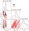 |
Fig. A.1. Corner plot of the model parameters of the MCMC result. Contours and histograms of BCG and CGM are shown in black and red, respectively. The off-diagonal panels show the joint distriburtion of each two parameters for BCG and CGM with contours showing [0.5, 1, 1.5, 2]σ levels. The diagonal panels show the histograms of all parameters including |
![Mathematical equation: $ \mathrm{\log{\frac{T_{kin}}{[K]}}} $](/articles/aa/full_html/2024/09/aa49642-24/aa49642-24-eq42.gif)
![Mathematical equation: $ \mathrm{\log{\frac{n_{H_2}}{[cm^{-3}]}}} $](/articles/aa/full_html/2024/09/aa49642-24/aa49642-24-eq43.gif)
All Tables
All Figures
|
Fig. 1. Submillimeter observations towards MACS1931. Upper left: Gaussian fit to the 12CO(1−0) line in the NRO 45-m observations of MACS1931. The black histogram shows the spectrum. The blue solid curve shows the Gaussian fit to the line. Upper right: Gaussian fit to the [CI](2−1) and 12CO(7−6) lines in the APEX observations of MACS1931. The black histogram shows the spectrum. The green and red solid curves show the Gaussian fits to the [CI](2−1) and 12CO(7−6) lines, respectively. The magenta solid lines show the regions of the spectrum excluded because of the atmospheric lines. Lower left: Best-fit line profiles of 12CO(1−0), 12CO(3−2), and 12CO(4−3) from Fogarty et al. (2019) (dashed curves) and Lorentzian fits on 12CO(1−0), 12CO(7−6), and [CI](2−1) from this work (solid curves) displayed on the same plot for comparison (see Sect. 3 and Table 1). The CGM tail peak of the 12CO(4−3) line from Fogarty et al. (2019) is the best fit to a partially truncated spectrum due to a spectral window gap in the ALMA Band 7 observations. Lower right: The ALMA 12CO(3−2) intensity map of the MACS1931 BCG and the tail. The moment zero map is calculated over a range of [ − 500, 600] km s−1. ALMA beam is shown by an ellipse on the bottom left side of the image. The APEX and NRO 45-m HPBWs are shown by solid red and dashed yellow circles. Contours are calculated on the moment map with levels [0.2, 0.5, 1, 2]σ and σ = 0.297 Jy beam−1 km s−1. The CGM tail component of the spectra is detectable in the [CI](2−1) line as well as all lines from Fogarty et al. (2019). |
| In the text | |
|
Fig. 2. CO SLED built with the available data for the BCG and the CGM tail of MACS1931 (red and orange stars, respectively). The CO line fluxes are taken from Fogarty et al. (2019), except 12CO(7−6) of the BCG which is detected in this work using APEX. Line fluxes are normalised to the 12CO(1−0) flux taken from Fogarty et al. (2019). Additional average CO SLEDs from the literature are added for comparison: ULIRGs from Papadopoulos et al. (2012a, blue circles), SMGs from Bothwell et al. (2013, green circles), BzK galaxies from Daddi et al. (2015, purple circles), low-redshift Herschel galaxies from Kamenetzky et al. (2016, magenta circles), and quasars from the QFeedS sample published in Molyneux et al. (2023, cyan circles). The dashed black line shows the theoretical CO SLED for resolved objects with ΣSFR = 0.83 M⊙ yr−1 kpc−2 modelled by Narayanan & Krumholz (2014). This value is the estimated ΣSFR for the MACS1931 BCG (Fogarty et al. 2015). The grey shaded area shows the predicted CO SLED range with this model for 0.6 < ΣSFR [M⊙ yr−1 kpc−2] < 3. We report an upper limit on the 12CO(7−6) flux for the tail in Table 2, however, it is not constraining the tail CO SLED and falls out of the range of this plot. |
| In the text | |
|
Fig. 3. Top: LVG modelling for the BCG of MACS1931. The Tkin, nH2 grid is plotted with a projected Kvir axis. At each point of the Tkin, nH2 grid, the colour shows the predicted [CI](2−1)/12CO(1−0) ratio of the model with the highest likelihood among models with different Kvir values. The black contours show the levels of the modelled [CI](2−1)/12CO(1−0) flux ratio which is shown by colours. The white contours show the likelihood levels. The white star indicates the best-fitted LVG model obtained from MCMC simulations. Bottom: The CO SLED of the best-fitted LVG model for BCG. The black curve shows the modelled CO SLED. The blue points with blue error bars show the observed line flux ratios. The green curves show the distribution of best models obtained from MCMC. |
| In the text | |
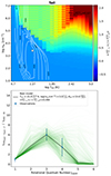 |
Fig. 4. LVG modelling and CO SLED for the CGM tail of MACS1931, similar to Figure 3. |
| In the text | |
|
Fig. A.1. Corner plot of the model parameters of the MCMC result. Contours and histograms of BCG and CGM are shown in black and red, respectively. The off-diagonal panels show the joint distriburtion of each two parameters for BCG and CGM with contours showing [0.5, 1, 1.5, 2]σ levels. The diagonal panels show the histograms of all parameters including |
| In the text | |
Current usage metrics show cumulative count of Article Views (full-text article views including HTML views, PDF and ePub downloads, according to the available data) and Abstracts Views on Vision4Press platform.
Data correspond to usage on the plateform after 2015. The current usage metrics is available 48-96 hours after online publication and is updated daily on week days.
Initial download of the metrics may take a while.