| Issue |
A&A
Volume 689, September 2024
|
|
|---|---|---|
| Article Number | A105 | |
| Number of page(s) | 21 | |
| Section | Cosmology (including clusters of galaxies) | |
| DOI | https://doi.org/10.1051/0004-6361/202449628 | |
| Published online | 06 September 2024 | |
The statistics of Rayleigh-Levy flight extrema
1
Université Paris-Saclay, CNRS, CEA, Institut de physique théorique, 91191 Gif-sur-Yvette, France
2
CNRS and Sorbonne Université, Institut d’Astrophysique de Paris, 98 bis Boulevard Arago, 75014 Paris, France
3
Korea Institute for Advanced Studies (KIAS), 85 Hoegi-ro, Dongdaemun-gu, Seoul 02455, Republic of Korea
Received:
16
February
2024
Accepted:
15
May
2024
Rayleigh-Levy flights have played a significant role in cosmology as simplified models for understanding how matter distributes itself under gravitational influence. These models also exhibit numerous remarkable properties that enable predictions of a wide range of characteristics. Here, we derive the one- and two-point statistics for extreme points within Rayleigh-Levy flights, spanning one to three dimensions (1D–3D) and stemming directly from fundamental principles. In the context of the mean field limit, we provide straightforward closed-form expressions for Euler counts and their correlations, particularly in relation to their clustering behaviour over long distances. Additionally, quadratures allow for the computation of extreme value number densities. A comparison between theoretical predictions in 1D and Monte Carlo measurements shows remarkable agreement. Given the widespread use of Rayleigh-Levy processes, these comprehensive findings offer significant promise not only in astrophysics, but also in broader applications beyond the field.
Key words: cosmology: theory / dark matter / large-scale structure of Universe
© The Authors 2024
 Open Access article, published by EDP Sciences, under the terms of the Creative Commons Attribution License (https://creativecommons.org/licenses/by/4.0), which permits unrestricted use, distribution, and reproduction in any medium, provided the original work is properly cited.
This article is published in open access under the Subscribe to Open model. Subscribe to A&A to support open access publication.
1. Introduction
The geometry and structure of cosmic fields form a complex physical system that develops from homogeneity through the interplay of expansion and long-range forces. Its statistical properties should emulate those of such a class of systems. From the perspective of observational cosmology, its evolution mirrors both the history of the universe’s expansion rate and the dynamic growth of embedded substructures (see e.g. Bardeen et al. 1986; Bernardeau et al. 2002, for an account of the emergence of structure due to gravitational instability). While the small-scale (galaxy-sized) structures are determined by the interaction of gravitational effects and complex baryonic physics, the large-scale structure is shaped solely by the development of the gravitational instabilities.
The most standard approach to describe the outcome of this evolution is to consider the matter correlation functions or (equivalently in Fourier space) the spectra (e.g. Peebles & Groth 1975; Fry 1985; Bernardeau 1994; Scoccimarro et al. 1998; Cappi et al. 2015). Those quantities capture however only partially the outcome of the gravitational processes. In particular gravitational instabilities leads to the formation of large scale structures, such as self-gravitating massive halos embedded in an intricate cosmic web made of voids, walls and filaments that are woven together under the influence of gravity (Bond et al. 1996). Inspired by such emerging features, a related alternative to quantify the properties of the field is to explore the topology of the excursion of the cosmic web. It can be done both in real space (e.g. Matsubara 1994; Gay et al. 2012) and redshift space (e.g. Matsubara 1996; Codis et al. 2013), using tools such as the void probability function (VPD, e.g. White 1979; Sheth & van de Weygaert 2004), the Euler-Poincaré characteristic (e.g. Gott et al. 1986; Park & Gott 1991; Appleby et al. 2018), or (more generally) Minkowski functionals (e.g. Mecke et al. 1994; Schmalzing & Buchert 1997), persistent homology (e.g. Sousbie et al. 2011; Pranav et al. 2017), and Betti numbers (e.g. Park et al. 2013; Feldbrugge et al. 2019). Given the duality established by Morse-Smale theory (Forman 2002) between the geometry or topology of excursion, and the loci of null gradients of the underlying density field, a summary statistics is given by the point process of these critical points (e.g. Bardeen et al. 1986; Bond et al. 1996; Gay et al. 2012; Cadiou et al. 2020). For instance, there has recently been some interest in also using the clustering of such points as cosmological probes (Baldauf et al. 2021; Shim et al. 2021), for instance, extracted from Lyman-α tomography (Kraljic et al. 2022). Unfortunately, the theory for capturing their statistics has been limited to the quasi Gaussian limit (e.g. Pogosyan et al. 2009), or slightly beyond (Bernardeau et al. 2015), while relying on the large deviation principle. This puts limitation on its realm of application to larger scales only (or involves relying on calibration over N-body simulations).
A notable cosmologically relevant counterexample is provided by Rayleigh-Levy flights1 (Mandelbrot 1975; Peebles 1980; Szapudi & Colombi 1996; Zimbardo & Perri 2013; Uchaikin 2019), which are simply defined as a Markov chain point process whose jump probability depends on some power law of the length of the jump alone. In 3D, it acts as a coarse proxy to describing the motion of dark halos (Sefusatti & Scoccimarro 2005; Trotta & Zimbardo 2015), but its definition can be extended to arbitrary dimensions. Rayleigh-Levy flights were first introduced in astrophysics by Holtsmark (1919) in the context of fluctuations in gravitational systems (Litovchenko 2021). They include some degree of connection to first-passage theory (Metzler 2019), underlying Press Schechter theory for halo formation (Press & Schechter 1974), and subsequent mass accretion (Musso et al. 2018). Rayleigh-Levy flights have also attracted lots of attention beyond cosmology, (from anomalous cosmic rays diffusion Wilk & Włodarczyk 1999; Boldyrev & Gwinn 2003, to ISM scintillation) or indeed beyond astronomy (from turbulence, Shlesinger et al. 1987; Sotolongo-Costa et al. 2000, to earthquakes), and even biology (e.g. Reynolds 2018) or risk management (e.g. Bouchaud & Potters 2003), as they captures anomalous diffusion (see e.g. Bouchaud & Georges 1990; Dubkov et al. 2008, and references therein).
Levy flights also provide an appealing playground with genuine scale-independent developed non-Gaussianities (that cannot be mimicked by a mere local nonlinear transformation of the fields), whose amplitudes resemble what is generally expected in gravitational density fields. These remarks would be of limited interest however if we had no way of exploring the statistical properties of such fields. Building on the early results of Peebles (1980) and of Bernardeau & Schaeffer (1999), Bernardeau (2022) derived a large corpus of properties of such fields. They were concerned to a large extend on the joint density probability distribution function (PDFs) at large separations.
In this paper, we focus on the local behaviour of the field, trying to first grasp the expected behaviour of the local density and its derivatives, so as to identify critical points in such a density field. The starting point of those investigations is based on the derivation of the cumulant generating function (CGF) in multiple cells. This allows us to predict their one and two point statistics to arbitrary order in the variance of the field. For clarity, the main text focuses on results, while all the derivations are given in the appendices.
Section 2 recalls the main relevant properties of Rayleigh-Levy flights. Section 3 presents the number count of extrema of flights in 1D, 2D, and 3D. Section 4 compute their clustering. Comparisons to Monte Carlo simulations are provided throughout for validation for the 1D flights. The companion paper will provide them for 2 and 3D flights. Section 5 presents our conclusions.
2. Rayleigh-Levy flight model
The random model, as introduced first in a cosmological context by J. Peebles (Peebles 1980), is defined as a Markov random walk where the PDF of the step length, ℓ, follows a cumulative distribution function given by:

where ℓ0 is a small-scale regularisation parameter. The random walks are dominated by rare, large events rather than the accumulation of many steps.
Calling f1(r) density of the subsequent point (the first descendant of a given point at position r0) at position r, we have:
where 𝒰sph(D) is the volume of a D-dimensional sphere of unit radius, 𝒰sph(D) = πD/2/Γ(D/2 − 1). For |r − r0|> ℓ0, it leads to

We then consider its Fourier transform, ψ(k) as:
The two-point correlation functions for Rayleigh-Levy flights between positions r1 and r2 is then given by
where n is the number density of points in the sample. When kl0 ≪ 1, then 1 − ψ(k)∼(ℓ0k)α, the large distance correlation function behaves as:
The expected behaviour of the large-distance correlation function is shown on Fig. 1 below, which clearly shows that this form is valid as soon as r ≥ ℓ0.
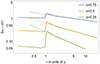 |
Fig. 1. Two-point correlation function for the 1D Rayleigh-Levy flights (before smoothing). The predictions are for ℓ0 = 1. The solid lines are the exact shapes derived from Eq. (5) exhibiting a clear exclusion zone for r < ℓ0. The dashed is the large scale asymptotic form. it can be observed that the exact solution converges very rapidly to the asymptotic form. |
We note that the numerical system is driven by two parameters, ℓ0 and n, with  . In practice one wants to make sure that the filtering scale is significantly larger than both ℓ0 and ℓn ≡ 1/n1/D and that the survey size, ℓ𝒮, is much larger than the filtering scale. When measuring the correlation properties of critical points, we also want to make sure that ℓ𝒮 is much larger than the scales at which the correlation functions are measured. It is always possible to meet these requirements, and reach any amplitude of ξ, provided there is access to enough resources to build Rayleigh-Levy flights with large number of points.
In practice, in the 1D numerical simulations we exploited, we have the following:
| α | = | 0.5 |
| n | = | 3/pixel |
| ℓ0 | = | 0.02 pixel |
| rG | = | 2 pixel |
| ℓ𝒮 | = | 105 pixel size |
| Nrealisations | = | 200 |
providing very accurate determination of all one-point quantities (density and critical points, etc.) and good estimates of their correlation, as shown below.
A key property of Rayleigh-Levy flights involves the structure of the higher order correlation functions. In such a model, not only are they known but they also display the type of behaviour that is generally expected in the context of cosmological models. We know from theory in the perturbative regime (Bernardeau et al. 2002), and to a large extend from observations (Yu & Hou 2022), that the p-order matter correlation functions scale like the power p − 1 of the two-point function. This assumption and its consequences are addressed in more details in Appendices A–C.
Conversely, from a theoretical perspective, the Rayleigh-Levy flights model falls within the class of models whose p-point correlation functions follow the so-called hierarchical Ansatz (Fry 1984), so that they can be expressed as a sum of products of two-point correlations:
This process actually embodies a more specific class of models, which correspond to cases where the Qp(t) values depend only on the vertex composition of the tree, that is,
where the vertices values, νq, are numbers associated with each vertex and depend only on their connectivity, q being the number of lines a given vertex is connected to (see Appendix B and Bernardeau & Schaeffer 1999). In the case of the flight models we consider here, we have only two non-zero vertices, ν1 and ν2, so that the trees we have to consider are, in fact, simply connected lines.
In general, the corresponding cumulant generating function of the underlying density field in cells of arbitrary profile given by 𝒲i(x) can be written as:
We note that in the Gaussian limit, this expression is restricted to terms with p1 + … + pn = 2. We also note that, in general, the full complexity of this expression is hard to exploit and can only be done in a perturbative sense, exploring, for instance, the consequences of terms at cubic order. This complexity is at the heart of the Edgeworth expansion (Kendall & Stuart 1977; Sellentin et al. 2017).
A remarkable property of the tree models in general, and of the Levy flight model in particular, is that the discrete summations that appear in this expression (over p1, …, pn), can be done explicitly. This is clearly an appealing feature of these models, as it allows for an exploration of their properties in a regime that can be arbitrarily far from the Gaussian case. This is the motivation for this study.
The details of the derivation of the resulting form for the CGF, φ(λ1, …, λn), is given in Appendix B, which shows that:
where τ(x) is the λi-dependent implicit solution of the consistency equation
Formally, τ(x) is actually the rooted-Cumulant Generating Function (the generating function of cumulants that originate from location x) and is denoted r-CGF hereafter. It will play an important role throughout this paper. The expression in Eq. (11) is the direct transcription of the tree model described by Eq. (8). It is the result of combinatoric computations, and does not rely on any approximation2. The practical implementation of Eq. (10) relies on some approximations, such as the mean field assumption, in which the r-CGF is assumed to remain constant within each cell (as detailed in Appendix B). This proves to be highly accurate for compact, non-compensated, spherically symmetric density profiles. Assuming it holds, we denote τi as the value of the r-CGF for each cell, i. We can then average Eq. (11) over the cell, i, with the profile 𝒲i(x), which leads to the following system
This becomes a set of n equations coupling the different values of τi. As can be seen here, in case of the present minimal tree model, this system is linear in τi. It can therefore be explicitly inverted3.
For the one-point cumulant generating function, Eq. (12) corresponds to the implicit equation:

where ξ0 is the average two-point correlation function within one cell:
The resulting CGF can easily be computed (See Appendix C):
Despite its apparent simplicity, this expression fully captures the whole cumulant hierarchy that we would expect for the density PDF. Furthermore, it turns out that the inverse Laplace transform of such an expression can be explicitly derived, see Bernardeau (2022) and Appendix C, and leads to the closed form expression of the density PDF:
The first (singular) term in Eq. (17) reflects the contribution to empty regions. The last terms involves the regularised confluent hypergeometric function,  , given by
  . We note that this model indeed predicts region that are empty even for an arbitrarily large number of points4. More specifically, the void probability function (VPDF) is non-zero, even in the continuous limit, and is given by

This feature can be appreciated on Fig. 2, where we can see empty regions that cover a large fraction of the sample. The VPDF can only be non-zero for a compact support filter, which not formally holds for a Gaussian filter. Yet the mean field result seems to accurately predict the VPDF for a top-hat filter. For a Gaussian filter, the behaviour of the density PDF in the low density regime is correct when corrections to the mean field solutions are included.
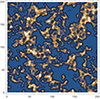 |
Fig. 2. Example of a 2D density field derived from a 2D levy flight. Parameters of the flight are α = 1., ℓ0 = 0.012 pixel size with ten points per pixel. The sample has periodic boundary conditions with 2002 pixels. The initial discrete (point) field has been convolved with a Gaussian window function of width of 2 (in pixel size) in each direction. The resulting variance as measured in the sample is 1.56. On the plot, the contour lines are log-spaced, from density of about 0.2–7. The deep blue regions correspond to empty regions. |
We note that for the mean-field solution, the dependence on the spatial dimension, the value of α and the filter shape is entirely contained in the value of ξ0. This is not the case for derivations of the density PDF beyond the mean-field solution, which are expected to depend on the details of the model and filtering schemes. Numerical investigations beyond the mean field show nonetheless that the high density tail of Eq. (17) is very robust. This is illustrated on Fig. 3, which displays the mean-field solution and its corrections in terms of Hermite polynomials (up to sixth order in the expression of the r-CGF, see Appendix C) and compares it to numerical results.
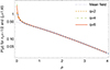 |
Fig. 3. Comparisons of measured density PDF from a set of 1D Rayleigh-Levy flights whose characteristics are given in the text, grey points, compared to different levels of theoretical predictions. The blue dotted line is the mean field approximation. The other lines correspond to different level of approximation, up to sixth order in an expansion in Hermite Polynomials. |
3. Critical point number counts
From a given realisation of the flight, a convolution by, for instance, a Gaussian filter allows us to define a smooth field, ρ, whose critical point can be studied statistically. The number density of critical points at a density, ρ, is then expressed as:
![$$ \begin{aligned} n_{\rm crit.}(\rho ) = \int \prod _{ij}{\mathrm{d}\rho _{\!,ij}} \mathrm{Sgn}\left[\rho _{\!,ij}\right]\! \det \left[\rho _{\!,ij}\right]\! P\!\left(\rho ,\rho _{\!,i}=0,\rho _{\!,ij}\right), \end{aligned} $$](/articles/aa/full_html/2024/09/aa49628-24/aa49628-24-eq23.gif)
where Sgn[ρ,ij] is either 0, 1 or −1, depending on the sign of the eigenvalues of the matrix, ρ,ij, to reflect the nature of the critical points considered. Hence, the computation of extrema densities requires the joint cumulant generating function of variables dual to the local density, its first and second order derivatives. Appendix D shows that it is indeed possible to derive such a joint CGF in the mean field limit. In short, the calculation is based on writing the mean field solution for a finite number of cells assumed to be infinitely close to one another; the derivatives are then obtained via finite differences.
Once the cumulant generating function for the field and its derivatives is known, the relevant conditional expectations are computed to predict the extrema and critical number counts and their clustering properties. We present below the results for the Euler and critical points in 1D–3D. As Eq. (19) involves up to the second derivative of the field, in principle, we should compute the joint PDF of the field and its derivative up to that order. In practice, For 1D Euler number counts, Appendix D shows explicitly that thanks to the stationarity of the field, only the first derivative is necessary, and we can write:
Overall, and after a significant amount of algebra, we derive in Appendix D the closed form Euler counts in ND:
where Pm and Qm are polynomials of order m in ρ and ξ1 is defined in Eq. (D.1). Specifically we find in Appendix D that


Here,  where the pre-factor defining ξ0 is a function of α only, given by Eqs. (A.7)–(A.9) for 1D–3D.
The simplicity of Eq. (21) is quite remarkable. We note, in particular, that for D = 2 to 3,  also does not involve ξ2 (see the discussion below and Appendix D).
We could speculate that relations, such as Eqs. (3)a–d, hold in higher dimensions, involving polynomials, Pi and Qi of increasing order, so that Eq. (21) mirrors the hierarchy for Gaussian random field Euler counts (involving Hermite polynomials, Adler & Taylor 2009), which follow from their cumulant generating functions given in Appendix F.
It is of interest to be able to distinguish between the number counts of maxima and minima separately. It turns out that the extrema counts can also be computed via specific (simple or double) numerical integration path in the complex plane as:
and
where χ1D(ρ; λxx) and χ2D(ρ; λκ, λγ) are given by Eqs. (D.34) and (D.51) respectively, while ϵ is a negative real constant for maxima and a positive real constant for minima. The 2D saddle counts follows from  .
.
To gain a bit of insight into these quantities, we consider the expression of  as a function of
  in the limit5γ → 0. The integrand in this case is greatly simplified and it leads to the same leading behaviour for the number density of maxima and minima given by:
which, as expected, scales like the inverse of typical distance between extrema, (ξ1/ξ2)1/2. The next to leading order is independent of γ, and corresponds to the Euler number density so that
where the dots represents subsequent terms in a γ expansion. Here nEuler is less sensitive to small scale high frequency features – or noise – compared to extrema number density. This is also the case for Gaussian field and for the Rayleigh-Levy flights in any dimension. Although we cannot demonstrate it, we speculate that this is true for all hierarchical models in which the high-order correlation function behave like products of the two-point correlations. Figures 4 and 5 present the corresponding number counts in 1D and 2D, respectively. In Fig. 4, in particular, we present a detailed comparison of the extrema, minima and Euler number densities as a function of the local density. We take advantage of the fact that we could rely on large number of realisations making the measurements of the critical points rather precise (numerical error bars due to the finite number of realisations are here negligible). For the 1D case, it is also rather simple to determine the position and type of critical points: they are obtained at locations where the local gradients (obtained after convolution on grid points shifted by 1/2 pixel) change sign from one pixel to the next. The type of critical point is simply given by the sign of the difference. Figure 4 shows that the theoretical predictions capture in exquisite details the measured densities of critical points. The only significant departure between the theoretical predictions and the numerical results is for the low density regime (ρ < 1), for the maxima number densities and to a less extent the minima number densities. These discrepancies are thought to be related to the breaking of the mean field approximation in the low density regime, as shown on Fig. 3 for the density PDF. All these conclusions are found to be valid irrespective of the details of the simulations (this is illustrated with a change of the value of α in the Rayleigh-Levy flights).
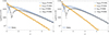 |
Fig. 4. Mean field predictions for extrema counts and comparison with 1D numerical Levy flight for two different indices as labelled. See text for details on the measurements. We note the Euler number density is negative on the low density branch as the number density of minima exceeds the number density of maxima. The agreement between theory and measurements is remarkable. |
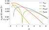 |
Fig. 5. Mean field prediction for extrema counts for 2D fields. The plots are for ξ0 = 1 and γ = 0.45. |
4. Clustering of critical points
One of the strength of analytical investigations of tree-hierarchical models is that the same re-summation techniques can be used to also infer the large distance correlation functions of the objects for which we can compute the number density. These calculations were pioneered in Bernardeau & Schaeffer (1999) for tree hierarchical models, applied also to the perturbation theory calculations in Bernardeau (1996), and more recently in Codis et al. (2016), Uhlemann et al. (2017), Munshi (2018), Repp & Szapudi (2021). A general thorough presentation of large-scale biasing is also to be found in the review paper by Desjacques et al. (2018).
The properties of large scale biasing were more specifically investigated in Bernardeau (2022) for the Rayleigh-Levy model, which focused on the consequences of this functional form for the covariance properties of density PDF measurements. These models share the same properties: the joint density PDF at large separation are expected to obey the following functional form
![$$ \begin{aligned} P(\rho _1,\rho _2)=P(\rho _1)P(\rho _2) \left[1+\xi (r_1,r_2)b(\rho _1)b(\rho _2)\right], \end{aligned} $$](/articles/aa/full_html/2024/09/aa49628-24/aa49628-24-eq39.gif)
where the densities ρ1 and ρ2 are taken at position r1 and r2 respectively. At this order, the dependence in the densities ρ1 and ρ2 factorises, making it possible to define a density bias function. In this paper, we present how such a relation can be extended to the number counts of critical points and derive the corresponding bias functions.
In Eq. (29) the bias function can be seen as the response function of the density PDFs to a change of the global density. This means that although the bias function cannot be derived from the density PDFs alone6, we should be able to derive it if an operational method is available to compute the density PDFs for arbitrary large-scale density (following the derivation of halo-bias function as pioneered by Mo & White (1996) in a separate universe approach). In hierarchical tree models, it can be computed making use of the r-CGF. The shape of the join density CGF at for densities at positions r1 and r2 written up to first order in ξ(r1, r2)/ξ0 indeed obeys

where τ1 is the r-CGF introduced in Eq. (11). The computation of the inverse Laplace transform of such a join CGF can be formally done at leading order in ξ(r1, r2) and has the functional form given by Eq. (29). More specifically, equation (16) is to be extended to
for the bias function. For the Rayleigh-Levy flights model, the large scale density bias function can be derived explicitly (Bernardeau 2022) and it is expressed as:
For a high density, its limiting behaviour is:
which corresponds to a dependence in  for high densities. We note that this is not a priori a generic result for hierarchical models and is at variance with the behaviour found in the context of Perturbation Theory calculations in Codis et al. (2016), where the bias at a high density is expected to be proportional to the density7.
The objective of this section is to present the correlation properties of the critical points of Rayleigh-Levy flights. Correlation properties of critical points will depend in general on i) the type of critical points we are considering and ii) the distance between the points and how this distance compares to the scale at which these points are defined. Despite the fact that the model we consider is unambiguously defined, it is near impossible to derive the correlation properties of critical points in their full complexity. Results can be derived at large enough separation and using the mean field approach, implying that our findings will be solid for large enough densities only.
The starting point is a generalisation of Equation (30) for the joint CGF of the density and its derivatives:

where λρ, {λi},{λij} are the conjugate variables of the density and its derivatives at a given location, μρ, {μi},{μij} those at a second location placed at distance, d, from one another. ξ0(d) is the filtered matter density correlation function at distance, d. This expansion is valid when d is much larger than the filtering scale and derived from the fact that we then expect ξ0(d)≪ξ0 and ξ2(d)/ξ2 ≪ ξ0(d)/ξ0 (see Appendix E). For the Rayleigh-Levy model we further have τ = ϕ. As for the density field this form implies a similar form for the two-point number density of the critical points:

where #i represents the types of critical points we consider and b#i(ρ) is the associated bias function whose expression is given by Eq. (E.7).
The computation of bias function of the critical points then makes use of the same techniques as for the number density. It does not lead to an explicit form for the extrema or saddle point position both in 1D and 2D. It is however possible to derive the explicit bias functions of the Euler points for the 1D and 2D case:
where the polynomials obey


Again one could conjecture that higher order polynomials exist for bias functions in higher dimensions. We note that bias functions in general are dimensionless quantities. They can therefore be expressed in terms of dimensionless quantities such as ξ0 and γ. Furthermore the bias parameter of Euler points is found to be also independent of ξ2 (as was the case for its number density) and therefore of γ.
The corresponding bias functions are shown in Fig. 6 and 7 in 1D and 2D, respectively. These functions are computed for ξ0 = 1 and for γ = 0.45, which corresponds roughly to what is expected for α = 0.5. The results however do not depend crucially on these specific choices.
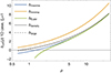 |
Fig. 6. Theoretical prediction for the bias function of 1D extrema, of Euler points and that of the local density, Eq. (32), and its corresponding large scale limit (dashed line) as given by Eq. (33). As expected, the maxima and Euler points have the same bias at a high density, this is also the bias of the density field itself: high density critical points are likely to be maxima of the fields and their correlation properties is to a large extent determine by density bias. |
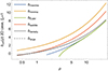 |
Fig. 7. Theoretical prediction for the bias function of 2D extrema, saddle points, Euler points and that of the local density (for which the predictions is the same as in 1D). Similar conclusions can be drawn from the 1D case. |
The functions exhibit some expected generic behaviours: (i) the high-density asymptotic behaviour of maxima and Euler points are the same. It also matches the asymptotic form of the local density bias: high-density regions tend to trace the locations of the maxima; (ii) for a given density, minima tend to be more correlated than saddle points or maxima: imposing to have a minima within a high-density region indeed requires an even higher density in the surroundings, which in turn translates into larger biases. One important conclusion that can be drawn here is that peak correlation properties derive, to a large extent, for the behaviour of the density bias functions in the sense of Eq. (29). This justifies to use such a proxy for the computation of peak correlation in the high-density regime for more involved models. Such an approach, however, cannot capture proximity or exclusion effects that would be expected for peak correlations.
To explore these effects specifically, we rely here on results from numerical experiments of 1D Rayleigh-Levy flights, for which accurate measurements can be achieved. The corresponding curves are presented on Figs. 8–12. To avoid too much numerical noise and uncertainties, they are expressed in terms of correlation function of cumulative quantities, where the local density is above a given threshold. More precisely the bias factors we will apply are defined as:
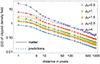 |
Fig. 8. Correlation function of the thresholded density regions and comparisons with predictions. The black solid line is the measured matter correlation function. The dashed lines are the prediction correlation amplitudes for thresholded regions derived from their large-scale limit. They have been computed after applying bias factors b#(> ρs)2 to ξ0(d) as measured in the simulation. |
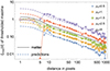 |
Fig. 9. Same as previous figure for the thresholded maxima. Open symbols correspond to negative values. We see a sharp transition between the large-scale behaviour – well predicted by the theory – and the small-scale behaviour. Note: the plateau at small scale corresponds to ξmax(d) = − 1, meaning that peaks generate an exclusion zone in their vicinity. |
 |
Fig. 10. Same as previous figure for the thresholded minima. We note that the minima are, as expected, more clustered than maxima for a given threshold value. We still observe a transition towards the small scale to ξmaxima(d) = − 1. We note that this measure is too noisy for a threshold ρs > 4. (not shown here). |
 |
Fig. 11. Same as previous figure for the thresholded Euler number densities. We still observe a transition towards the small scale. We note that here ξEuler(d) < − 1 showing that minima and maxima tend to be correlated at small distance (as confirmed in the next plot). Note: this measure is quite noisy as the Euler number density vanishes for low thresholded values and the threshold ρs > 0.5 is not shown. |
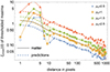 |
Fig. 12. Cross-correlation between minima and maxima with the same threshold. The prediction is obtained here by multiplying ξ0(d) as measured in the simulation by bmin(> ρs)bmax(> ρs). We note a large positive correlation for scales that are of the order of the smoothing scale. |
The 1D correlation functions are directly computed in position space by applying a simple shift to the density fields. No binning is applied and they are measured to a separation of 1000 pixels, which is safely smaller than the sample size.
Fig. 8 shows the correlation functions of the thresholded density for different thresholds. The dashed lines are the theoretical predictions, namely, the expectation when one multiplies the measured matter correlation function of the filtered density field (grey solid line) with b(> ρs)2. One can see that proximity effects tend to be rather insignificant for low density threshold, but rather large for high density threshold: for ρs = 4 proximity effects can be detected up to a distance of about 100 pixels. We can also predict the actual shape of the two-point function for Rayleigh-Levy flights models. This is presented in Fig. 1.
Figures 8–11 display their corresponding clipped two-point functions, while Fig. 12 shows the cross correlation of minima and maxima. The consistency of the results with theoretical predictions show that on large scales, the functional form of the peak biases, Eq. (35), is indeed satisfied, and the auto- and cross correlation properties of critical points can be described with such a factorised form.
5. Discussion and conclusions
Rayleigh-Levy flights can serve as numerical models portraying matter distribution within highly nonlinear fields in cosmology. In contrast to standard Markovian processes, Rayleigh-Levy flights display long-range correlations across all orders, which are precisely understood. Thus, these models serve as simplified representations, capturing statistical properties of the cosmic density field after gravitational instabilities reach its full development, although we are well aware they do not precisely replicate the outcomes of these instabilities. Despite this, they exhibit key properties, such as hierarchical structure in the higher correlation functions, making their study a valuable reference point.
We wish to emphasise that Rayleigh-Levy flights differ from simple nonlinear transformations (like a lognormal fields introduced by Coles & Jones 1991, which are now widely used as toy models), as they exhibit hierarchical properties across scales. This makes them the only known example (at least to us) of an actual random process whose outcome displays the expected scaling properties in correlation functions. Although it exhibits such a non-trivial structure, it is yet simple enough to allow for a wide range of explicit predictions.
Utilising the mean field approximation specifically enables the derivation of closed analytical forms for crucial parameters, such as Euler number densities and their correlations across significant separations: Eqs. (21) and (36), along with corresponding quadratures for extreme value counts, represent the primary outcomes of this study. Importantly, our predictions hold irrespective of the density field’s variance. While aligning with expectations for a Gaussian field in the regime of small variances, our numerical experiments confirm their validity across all variance values. Several key insights emerge from our findings:
-
The critical point density depends8 on three quantities related to density variance, gradient variance, and variance of the second-order derivative, denoted as ξ0, ξ1, and ξ2, respectively. These can be re-expressed using two dimensionless parameters, ξ0 and
 , along with ξ1, inversely proportional to distance squared. This implies that number densities scale as
  in N dimensions. Remarkably, while extrema number counts are correlated with both ξ0 and γ, Euler number counts remain independent of γ. This hints at the impact of small-scale features on peak counts, creating pairs of peaks and troughs at roughly the same height, ultimately leaving Euler number densities unaffected. We speculate that this property may extend to all hierarchical models.
 -
Concerning point correlations, akin to matter fields, we find that critical points of all types exhibit a factorised structure in the large separation limit, as given in Eq. (35). This pattern resembles the separate universe approach and has been validated through our numerical experiments. It enables the derivation of bias parameters for various types of points, especially as given in Eq. (36).
-
Notably, bias parameters of maxima, Euler points, and threshold-limited density fields converge to the same limit in the high-density limit. This suggests that regions with rare high-density values likely host one extremum, sharing identical correlation properties in this limit. This supports simplified approaches where peak correlations mirror those of high-density regions in more complex systems (see e.g. Bernardeau & Schaeffer 1999).
Beyond the paper’s scope, extending Eqs. (21), (26), and (36) to higher dimensions, other Minkowski functionals, and cross-validating them via Monte Carlo techniques, as done in 1D, will prove valuable and will be the topic of upcoming papers. One interesting line of investigation is for instance to use these results as benchmarks for validating quasi-Gaussian expansion schemes. It could also be contrasted with those derived in the large deviation limit (as presented in Uhlemann et al. 2016). Furthermore, these statistics may find application in analyzing the influence of Rayleigh-Levy flights in anomalous diffusive processes (e.g. in supersonic turbulence, Colbrook et al. 2017) or finite star effects in gravitating systems (Chavanis 2009).
Given their common occurrence, the comprehensive findings from this study hold promise not just in astrophysics but also in broader applications beyond the field.
Data availability
The data underlying this article will be shared on reasonable request to the corresponding author. Some of the codes underpinning this paper are available on Github at the following URL: https://github.com/cncpichon/levyflight
See Klages et al. (2008) for a fairly recent review.

To be more precise, the Rayleigh-Levy flights model leads to identical CGF and r-CGF, whereas these two functions are expected to exhibit different singularities on the real axis for generic tree model, as shown by Bernardeau & Schaeffer (1999).
They also depend on the specificities of the model through structural quantities encoded for instance in the scale cumulant generating function in the context of the large-deviation principle, (see e.g. Bernardeau & Reimberg 2016).
for time translation invariance such processes are called stationary, as explored in Adler & Taylor (2009).
Indeed, geometrically, adding high-frequency low-amplitude noise to a ND field, while creating new extrema, will also introduce saddle points along the new persistent ridges (ascending or descending 1D manifolds) linking them to existing extrema (Cadiou et al. 2024). This will not change the  of the field, since the signature of the new paired points only differ by one, so their contributions cancel. This in turn suggests that ξ2 does not contribute to
  .
.
Acknowledgments
We warmly thank S. Appleby for feedback and numerical checks in 2 and 3D. We also thank D. Pogosyan for comments and for updating his extrema count codes to suit our purpose, T. Abel for interesting feedback and Patrick Peter for typographic advice. We are grateful for the KITP for hosting the workshop https://www.cosmicweb23.org during which this project was advanced. This work is partially supported by the National Science Foundation under Grant No. NSF PHY-1748958. This work has made use of the Horizon cluster hosted by the Institut d’Astrophysique de Paris. We also thank S. Rouberol for running it smoothly.
References
- Adler, R. J., & Taylor, J. E. 2009, Random Fields and Geometry (New York: Springer) [Google Scholar]
- Appleby, S., Park, C., Hong, S. E., & Kim, J. 2018, ApJ, 853, 17 [NASA ADS] [CrossRef] [Google Scholar]
- Baldauf, T., Codis, S., Desjacques, V., & Pichon, C. 2021, Phys. Rev. D, 103, 083530 [CrossRef] [Google Scholar]
- Balian, R., & Schaeffer, R. 1989, A&A, 220, 1 [NASA ADS] [Google Scholar]
- Bardeen, J. M., Bond, J. R., Kaiser, N., & Szalay, A. 1986, ApJ, 304, 15 [NASA ADS] [CrossRef] [Google Scholar]
- Bernardeau, F. 1994, ApJ, 433, 1 [NASA ADS] [CrossRef] [Google Scholar]
- Bernardeau, F. 1996, A&A, 312, 11 [NASA ADS] [Google Scholar]
- Bernardeau, F. 2022, A&A, 663, A124 [NASA ADS] [CrossRef] [EDP Sciences] [Google Scholar]
- Bernardeau, F., & Reimberg, P. 2016, Phys. Rev. D, 94, 063520 [NASA ADS] [CrossRef] [Google Scholar]
- Bernardeau, F., & Schaeffer, R. 1992, A&A, 255, 1 [NASA ADS] [Google Scholar]
- Bernardeau, F., & Schaeffer, R. 1999, A&A, 349, 697 [NASA ADS] [Google Scholar]
- Bernardeau, F., Colombi, S., Gaztañaga, E., & Scoccimarro, R. 2002, Phys. Rep., 367, 1 [Google Scholar]
- Bernardeau, F., Codis, S., & Pichon, C. 2015, MNRAS, 449, L105 [NASA ADS] [CrossRef] [Google Scholar]
- Boldyrev, S., & Gwinn, C. 2003, ApJ, 584, 791 [NASA ADS] [CrossRef] [Google Scholar]
- Bond, J. R., Kofman, L., & Pogosyan, D. 1996, Nature, 380, 603 [NASA ADS] [CrossRef] [Google Scholar]
- Bouchaud, J.-P., & Georges, A. 1990, Phys. Rep., 195, 127 [CrossRef] [Google Scholar]
- Bouchaud, J.-P., & Potters, M. 2003, Theory of Financial Risk and Derivative Pricing, 168 [CrossRef] [Google Scholar]
- Cadiou, C., Pichon, C., Codis, S., et al. 2020, MNRAS, 496, 4787 [Google Scholar]
- Cadiou, C., Pichon-Pharabod, E., Pichon, C., & Pogosyan, D. 2024, MNRAS, 531, 1385 [NASA ADS] [CrossRef] [Google Scholar]
- Cappi, A., Marulli, F., Bel, J., et al. 2015, A&A, 579, A70 [NASA ADS] [CrossRef] [EDP Sciences] [Google Scholar]
- Chavanis, P. H. 2009, Eur. Phys. J. B, 70, 413 [NASA ADS] [CrossRef] [Google Scholar]
- Codis, S., Pichon, C., Pogosyan, D., Bernardeau, F., & Matsubara, T. 2013, MNRAS, 435, 531 [NASA ADS] [CrossRef] [Google Scholar]
- Codis, S., Bernardeau, F., & Pichon, C. 2016, MNRAS, 460, 1598 [NASA ADS] [CrossRef] [Google Scholar]
- Colbrook, M. J., Ma, X., Hopkins, P. F., & Squire, J. 2017, MNRAS, 467, 2421 [NASA ADS] [CrossRef] [Google Scholar]
- Coles, P., & Jones, B. 1991, MNRAS, 248, 1 [NASA ADS] [CrossRef] [Google Scholar]
- Desjacques, V., Jeong, D., & Schmidt, F. 2018, Phys. Rep., 733, 1 [Google Scholar]
- Dubkov, A. A., Spagnolo, B., & Uchaikin, V. V. 2008, Int. J. Bifurc. Chaos, 18, 2649 [NASA ADS] [CrossRef] [Google Scholar]
- Feldbrugge, J., van Engelen, M., van de Weygaert, R., Pranav, P., & Vegter, G. 2019, JCAP, 2019, 052 [CrossRef] [Google Scholar]
- Forman, R. 2002, Sém. Lothar. Combin., 48, 35 [Google Scholar]
- Fry, J. N. 1984, ApJ, 279, 499 [NASA ADS] [CrossRef] [Google Scholar]
- Fry, J. N. 1985, ApJ, 289, 10 [NASA ADS] [CrossRef] [Google Scholar]
- Gay, C., Pichon, C., & Pogosyan, D. 2012, Phys. Rev. Lett., 85, 023011 [NASA ADS] [Google Scholar]
- Gott, J., Richard, I., Melott, A. L., & Dickinson, M. 1986, ApJ, 306, 341 [NASA ADS] [CrossRef] [Google Scholar]
- Holtsmark, J. 1919, Ann. Phys., 363, 577 [CrossRef] [Google Scholar]
- Janninck, G., & des Cloizeau, J., 1987, Les polymères en solution (Les Ulis, France: Les éditions de physique) [Google Scholar]
- Kendall, M., & Stuart, A. 1977, The Advanced Theory of Statistics. Distribution Theory, 1 (New York: Macmillan Publication Co, Inc) [Google Scholar]
- Klages, R., Radons, G., & Sokolov, I. M. (eds.) 2008, Anomalous Transport (New York: Wiley) [CrossRef] [Google Scholar]
- Kraljic, K., Laigle, C., Pichon, C., et al. 2022, MNRAS, 514, 1359 [NASA ADS] [CrossRef] [Google Scholar]
- Litovchenko, V. A. 2021, Ukrain. Math. J., 73, 76 [CrossRef] [Google Scholar]
- Mandelbrot, B. 1975, Academie des Sciences Paris Comptes Rendus Serie Sciences Mathematiques, 280, 1551 [NASA ADS] [Google Scholar]
- Matsubara, T. 1994, ApJ, 434, L43 [NASA ADS] [CrossRef] [Google Scholar]
- Matsubara, T. 1996, ApJ, 457, 13 [NASA ADS] [CrossRef] [Google Scholar]
- Mecke, K. R., Buchert, T., & Wagner, H. 1994, A&A, 288, 697 [NASA ADS] [Google Scholar]
- Metzler, R. 2019, J. Stat. Mech. Theory Exp., 2019, 114003 [NASA ADS] [CrossRef] [Google Scholar]
- Mo, H. J., & White, S. D. M. 1996, MNRAS, 282, 347 [Google Scholar]
- Munshi, D. 2018, JCAP, 2018, 053 [CrossRef] [Google Scholar]
- Musso, M., Cadiou, C., Pichon, C., et al. 2018, MNRAS, 476, 4877 [Google Scholar]
- Park, C., Gott, J. R. I., 1991, ApJ, 378, 457 [NASA ADS] [CrossRef] [Google Scholar]
- Park, C., Pranav, P., Chingangbam, P., et al. 2013, J. Korean Astron. Soc., 46, 125 [CrossRef] [Google Scholar]
- Peebles, P. J. E. 1980, The Large-scale Structure of the Universe (Princeton: Princeton University Press) [Google Scholar]
- Peebles, P. J. E., & Groth, E. J. 1975, ApJ, 196, 1 [NASA ADS] [CrossRef] [Google Scholar]
- Pogosyan, D., Gay, C., & Pichon, C. 2009, Phys. Rev D, 80, 081301 [NASA ADS] [CrossRef] [Google Scholar]
- Pranav, P., Edelsbrunner, H., van de Weygaert, R., et al. 2017, MNRAS, 465, 4281 [Google Scholar]
- Press, W. H., & Schechter, P. 1974, ApJ, 187, 425 [Google Scholar]
- Repp, A., & Szapudi, I. 2021, MNRAS, 500, 3631 [Google Scholar]
- Reynolds, A. M. 2018, J. Phys. Commun., 2, 085003 [NASA ADS] [CrossRef] [Google Scholar]
- Schmalzing, J., & Buchert, T. 1997, ApJ, 482, L1 [NASA ADS] [CrossRef] [Google Scholar]
- Scoccimarro, R., Colombi, S., Fry, J. N., et al. 1998, ApJ, 496, 586 [NASA ADS] [CrossRef] [Google Scholar]
- Sefusatti, E., & Scoccimarro, R. 2005, Phys. Rev. D, 71, 063001 [NASA ADS] [CrossRef] [Google Scholar]
- Sellentin, E., Jaffe, A. H., & Heavens, A. F. 2017, ArXiv e-prints [arXiv:1709.03452] [Google Scholar]
- Sheth, R. K., & van de Weygaert, R. 2004, MNRAS, 350, 517 [NASA ADS] [CrossRef] [Google Scholar]
- Shim, J., Codis, S., Pichon, C., Pogosyan, D., & Cadiou, C. 2021, MNRAS, 502, 3885 [NASA ADS] [CrossRef] [Google Scholar]
- Shlesinger, M. F., West, B. J., & Klafter, J. 1987, Phys. Rev. Lett., 58, 1100 [NASA ADS] [CrossRef] [Google Scholar]
- Sotolongo-Costa, O., Antoranz, J. C., Posadas, A., Vidal, F., & Vázquez, A. 2000, Geophys. Res. Lett., 27, 1965 [NASA ADS] [CrossRef] [Google Scholar]
- Sousbie, T., Pichon, C., & Kawahara, H. 2011, MNRAS, 414, 384 [NASA ADS] [CrossRef] [Google Scholar]
- Szapudi, I., & Colombi, S. 1996, ApJ, 470, 131 [NASA ADS] [CrossRef] [Google Scholar]
- Trotta, E. M., & Zimbardo, G. 2015, J. Plasma Phys., 81, 325810108P [CrossRef] [Google Scholar]
- Uchaikin, V. V. 2019, Phys. Astron. Int. J., 3, 82 [CrossRef] [Google Scholar]
- Uhlemann, C., Codis, S., Kim, J., et al. 2016, MNRAS, 466, 2067 [Google Scholar]
- Uhlemann, C., Codis, S., Kim, J., et al. 2017, MNRAS, 466, 2067 [NASA ADS] [CrossRef] [Google Scholar]
- White, S. D. M. 1979, MNRAS, 186, 145 [NASA ADS] [CrossRef] [Google Scholar]
- Wilk, G., & Włodarczyk, Z. 1999, Nucl. Phys. B Proc. Suppl., 75, 191 [NASA ADS] [CrossRef] [Google Scholar]
- Yu, H., & Hou, X. 2022, Astron. Comput., 41, 100662 [NASA ADS] [CrossRef] [Google Scholar]
- Zimbardo, G., & Perri, S. 2013, ApJ, 778, 35 [CrossRef] [Google Scholar]
Appendix A: Rayleigh-Levy flight model
The random Rayleigh-Levy flights model was introduced first (in a cosmological context) by J. Peebles (Peebles 1980). This is a Markov random walk where the PDF of the step length ℓ follows a cumulative cumulative distribution function given by Eq. (2), where ℓ0 is a small-scale regularisation parameter. As a result, the density of the subsequent point (first descendant) at position r is given by:
Defining ψ(k) as the Fourier transform of f1(r) with Eq. (4), we can easily show that when assuming there are an infinity of points in the flight, the density in r of descendants of the point at position r0 is given by a series of convolutions whose resummation is:
The two-point density correlation function is then given by two possible configurations: a neighbourg can either be an ascendant or a descendant, so that the two-point correlation functions between positions r1 and r2 are given by
![$$ \begin{aligned} \xi _{2}(\boldsymbol{r}_{1},\boldsymbol{r}_{2})&=\frac{1}{n}\left[f(\boldsymbol{r}_{1},\boldsymbol{r}_{2})+f(\boldsymbol{r}_{2},\boldsymbol{r}_{1})\right], \end{aligned} $$](/articles/aa/full_html/2024/09/aa49628-24/aa49628-24-eq60.gif)
where n is the number density of points in the sample which leads to Eq. (5) of the main text. We note that the two-point correlation within the sample is therefore scaled as 1/n. The latter can be associated with a typical length, ℓn,

At large distance (compared to ℓ0), we expect the two-point correlation to behave as power laws. They are given by
For practical purposes, we give here the resulting expression of the average correlation, ξ0, for a Gaussian window function of width rs,
The main interest of this model however lies in the fact that its higher order correlation functions can also be computed and that they take a simple form. The reason is that n points are correlated when they are embedded in a chronological sequence (that can be run in one direction or the other). Thus the three-point function is simply given by
![$$ \begin{aligned} \xi _{3}(\boldsymbol{r}_{1},\boldsymbol{r}_{2},\boldsymbol{r}_{3})=\frac{1}{n^{2}}\left[f(\boldsymbol{r}_{1},\boldsymbol{r}_{2})f(\boldsymbol{r}_{2},\boldsymbol{r}_{3})+...\right] ,\end{aligned} $$](/articles/aa/full_html/2024/09/aa49628-24/aa49628-24-eq68.gif)
with five other terms obtained by all permutations of the indices. Expressing the result in terms of the two-point function, we have
![$$ \begin{aligned} \xi _{3}(\boldsymbol{r}_{1},\boldsymbol{r}_{2},\boldsymbol{r}_{3})&=\frac{1}{2}\left[\xi _{2}(\boldsymbol{r}_{1},\boldsymbol{r}_{2})\xi _{2}(\boldsymbol{r}_{2},\boldsymbol{r}_{3})+\right.\nonumber \\&\left.\xi _{2}(\boldsymbol{r}_{2},\boldsymbol{r}_{3})\xi _{2}(\boldsymbol{r}_{3},\boldsymbol{r}_{1})+\xi _{2}(\boldsymbol{r}_{3},\boldsymbol{r}_{1})\xi _{2}(\boldsymbol{r}_{1},\boldsymbol{r}_{2}) \right] .\end{aligned} $$](/articles/aa/full_html/2024/09/aa49628-24/aa49628-24-eq69.gif)
The type of expansion can be pursued to any order. The resulting shapes of the p-point correlation function is the following:
![$$ \begin{aligned} \xi _{p}(&\boldsymbol{r}_{1},\cdots \boldsymbol{r}_{p})=\frac{1}{n^{p-1}} \!\!\!\!\!\sum _{\sigma \in \mathrm{perm}[p]}\!\! f(\boldsymbol{r}_{\sigma _{1}},\boldsymbol{r}_{\sigma _{2}})\dots f(\boldsymbol{r}_{\sigma _{n-1}},\boldsymbol{r}_{\sigma _{n}})\,, \nonumber \end{aligned} $$](/articles/aa/full_html/2024/09/aa49628-24/aa49628-24-eq70.gif)
where σ is any permutation of the p indices 1, …, p. It implies that the p-point correlation function can be expressed in terms of the two-point functions
![$$ \begin{aligned} \xi _{p}(&\boldsymbol{r}_{1},\cdots \boldsymbol{r}_{p})=\left(\frac{1}{2}\right)^{p-2} \!\!\!\!\! \sum _{\sigma \in \mathrm{perm^*}[p]}\!\!\!\!\!\!\!\xi _{2}(\boldsymbol{r}_{\sigma _{1}},\boldsymbol{r}_{\sigma _{2}})\dots \xi _{2}(\boldsymbol{r}_{\sigma _{n-1}},\boldsymbol{r}_{\sigma _{n}}), \nonumber \end{aligned} $$](/articles/aa/full_html/2024/09/aa49628-24/aa49628-24-eq71.gif)
where the exponent refers to the subset of permutations that lead to a unique un-oriented sequence; identifying, for instance, Eqs. (1, 2, 3) and (3, 2, 1)). As we see hereafter it corresponds to a specific hierarchical tree model.
Appendix B: Hierarchical tree models
The Rayleigh-Levy flight model is one representative of a large class of models, the so-called hierarchical tree models, that have been put forward in cosmology as a way to model the density field in the highly nonlinear regime. Such models are presented in detail in Bernardeau & Schaeffer (1999). We recall here how they are defined, together with the basic equation that allows the derivation of their cumulant-generating function. Hierarchical tree models are a general class of non-Gaussian fields whose n-point correlation functions, ξp(r1, …, rp), follow the so-called hierarchical Ansatz,
where ξ(ri, rj) is the two-point function, while the sum is made over all possible trees that join the p points (diagram without loops), and the tree value, Qp, is obtained by the product of a fixed weight (that depends only on the tree’s topology), and the product of the two-point correlation functions, for all pairs that are connected together in the given tree. More specifically it is assumed that:
where νp is a weight attributed to all vertices with p incoming lines (assuming ν0 = ν1 = 1 for completion). In this formalism, the vertex generating function is generally introduced as:
Such models are thus entirely defined by i) the two-point functions ξ(r) and ii) the vertex-generating function ζ(τ). What the previous section has shown is that the Rayleigh-Levy flight model (in the continuous limit) corresponds, in the continuous limit, to a specific hierarchical tree model9 with ν2 = 1/2, νq = 0 for q ≥ 3.
B.1. Expression for cumulant generating function
The exact generating function of multiple cell correlation functions can be built through simple transforms. We hereafter consider a set of n cells i of profile 𝒲i(x), thus allowing for generic types of profiles, and not only top-hat boxes as was assumed in early papers. These profiles can obviously overlap but they are assumed to be well localised. The joint cumulants we consider in this formalism are those of the average densities in cells i that can be expressed in terms of spatial averages of correlation functions:
We then wish to build the cumulant-generating function (CGF) of the densities in each cells. It is given by:
This function represents the generating function of (averaged) cumulants, where the power of the λi counts the number of points in each cells. When the cumulants follow the tree structure described in the previous paragraph, each term that appear in this function then corresponds to a specific tree. Following a method pioneered by Janninck (1987), Bernardeau & Schaeffer (1992) showed that it is actually possible to perform the summation over such a set of trees, leading to a formal expression we re-derive briefly below.
To do so, we first now define a larger class of objects, ϕ[νp(x),ξ(x, x′)] (note the different symbol), which represents the sum of trees with vertices of order p having the weight νp(x) and lines having the weight ξ(x, x′), and where x are space variables that are subsequently integrated in the whole domain. In the context of tree theory, a point that reaches a one-point vertex ν1(x) are usually called a ’leaf’. The function we are interested in, φ(λ1, …, λn), is precisely equal to ϕ[νp(x),ξ(x, x′)] for the specific choice:
We now consider ϕ[νp(x),ξ(x, x′)] as a function of ν1(x) only, with the other quantities it depends on being fixed. We can then define τ(x) as the functional derivative of ϕ with respect to ν1(x):
Then τ(x) appears to be the generating function of all trees with (at least) one leaf at position x. This is a sub-part of rooted-trees10, and we therefore call τ(x) the rooted-Cumulant Generating Function (r-CGF). The key relevant property is then that τ(x) obeys a consistency relation, as it can be built recursively: when a line emerges from position x, it should reach a vertex of order p ≥ 1 at position x′ which is then connected to p − 1 r-CGFs at position x′. The mathematical transcription of the property is that
Once τ(x) is known, solving for ϕ then simply involves integrating Eq. (B.8). This can be done with the help of its Legendre transform with respect to ν1(x). Defining ψ as a functional of τ(x) via
the relation (B.8) is satisfied when
![$$ \begin{aligned} \frac{\delta \psi [\tau (\boldsymbol{x})]}{\delta \tau (\boldsymbol{x})} =\nu _1(\boldsymbol{x})\,. \end{aligned} $$](/articles/aa/full_html/2024/09/aa49628-24/aa49628-24-eq82.gif)
As ξ(x, x′) is a definite positive operator, the relation (B.9) can be inverted for ν1(x) as
and formally integrated via Eq. (B.11) into
with the correct boundary conditions (it should vanish when ν1(x) does). From Eq. (B.10), the function ϕ is then expressed as:
which solves the formal calculation. We can then apply this result for our specific setting (using Eq. B.7) to derive the CGF we are interested in. It is then convenient to re-express τ(x) in Eq. (B.13) in terms of the ζ function (Eq. B.3), the profiles, 𝒲i(x), and the λi variables. It eventually yields the following expression:
and the equation for the r-CGF function reads:
The expressions presented in the main text, Eqs. (10) and (11), are obtained for the specific expression of ζ corresponding to the Rayleigh-Levy flight statistics; namely, ζ(τ) = (1 + τ/2)2. The generic expression for the multiple CGF of hierarchical tree models was presented in Bernardeau & Schaeffer (1999).
B.2. Mean field equation
To make the resolution of the implicit Eqs. (11) more tractable, it is possible to assume that within each cell, τ(x) can be approximated by a constant equal to τi. The consistency equations for the τis, Eq. (11) is then expressed as:
where ξij is the average density correlation between cells i and j,
From Eq. (10), we then have
This is the form we will mostly use in the main text.
Appendix C: Minimal tree model
The minimal tree model (MTM) is defined as a tree model for which only vertices with two outcoming lines exist. It is therefore associated with a vertex generating function of the form:
It has been shown (in Balian & Schaeffer 1989, from the behaviour of the void probability function) that the only possible value for ν2 is ν2 = 1/2. This is precisely the case of the Rayleigh Levy flight model. From Eq. (C.1), this model is thus characterised by
In this case the stationary equations for a set of cells, Eq. (B.16) is expressed as:

and Eq. (B.18) becomes
As the right hand side of Eq. (C.3) is linear in τ, this system can be solved by the simple inversion of a matrix. In practice it is therefore relatively easy to derive the expression of τi (and therefore of the cumulant generating function) for a finite number of cells.
C.1. Mean field solution
From Eqs. (C.3)-(C.4) when only one cell is considered, the one-point mean field solution turns out to be
It gives the expression of the CGF for a single variable ρ of mean unity and mean square ξ0. The successive reduced cumulants of such a quantity can be easily computed by Taylor expansion.
We note that if the random variable ρ is rescaled to have a mean of  (instead of 1), its CGF is
  , which, given Eq. (C.5), is equal to
  .
.
C.2. MTM composition law and scale convolution
We generically define the cumulant generating function, φn({λi};{ξij}), of a set of n cells, of variables λi for cells whose two-point correlations are ξij. Then the following identity is satisfied by φn:

This important scaling, which we use continuously throughout, may seem at first view as an awkward relation, as it states that the ξ in φn can be shifted by successive application of the function φ1. This result seems specific to Rayleigh-Levy flights.
We first briefly demonstrate the property. To avoid confusion in the notation, we define τi and  as the solutions of the following systems:
Then we also define μi and  as μi = 1 + τi/2 and
  so that
Then  is the only solution of the system
where the matrix Mij is defined as
Now, since
this implies that  is the solution of Eq. (C.11), so that by identification we have:
Hence,
which establishes the relation.
Equation (C.6) reflects some interesting physical properties it is related to: scale composition when cell correlations are built as a two-steps procedure. Indeed, we consider a set of random Rayleigh-Levy flights experiments, in which instead of having of fixed number of points in each sample, the sample density is itself drawn from the one-point PDF derived from an MTM process. We denote ρs the sample density (whose average is set to unity). Its CGF is then φ1(λs; ξs), where ξs is the variance of the sample density.
We then note that for each realisation the cell densities, ρi scale like 1/ρs (by definition ρi is defined with respect to the mean of the survey) and that its correlation functions ξij scale like 1/ρs (this is a consequence of the expression of the scaling of the two-point function in the Rayleigh Levy model). To be more precise, we define  as the cell correlations when the sample density is equal to unity. We then have

We then define the densities  which represent the ‘true’ density in the sample (that is when the sample density is taken into account) as:

and aim at building the joint PDF of  . This PDF is formally given by
where the dependence in ρs is also present in the expression of ξij. Then, making the change of variable

and noting that:

we have
Now the integral over ρs leads to a Dirac delta function in  leading to
This expression means formally that the CGF of  is this two-step construction given by
  . The relation (C.6) ensures that it is also given by
  , which states that survey density fluctuations can, in this model, be taken into account via a simple shift in the cell correlation amplitudes.
A useful practical consequences of property (C.6) is that we could set any peculiar element of ξij to zero. For instance, the CGF of two identical cells of density variance  and of cross-correlation ξ12 is given by:

It is possible to extend such a construction for a larger number of cells11, but for specific configurations only. Note finally that when one needs to construct the density CGF for a large number of cells it is convenient to set  for all cells as it makes the system in τi sparser.
C.3. Computing PDF in the minimal tree model
The basic quantity one wishes to have access to is the PDF, defined as the inverse Laplace transform of the cumulant generating function φ1(λρ), that is,
where the integral runs formally along the imaginary axis, but can be moved in the complex plane as long as no poles or singularities are encountered along the path.
The following relation will be exploited throughout this paper

where  is the 1D Dirac distribution and
  is the regularised confluent hypergeometric function 0F1(a; z)/Γ(a). This formula can be applied directly to φ1(λρ; ξ0) to derive P(ρ). It can also be applied after successive derivatives with respect to ac from which on can establish that
for n ≥ 1. Then, the application of Eq. (C.24) to Eq. (C.5) leads to:
which yields the PDF in the mean field approximation. One can see that it involves the sum of two terms, a Dirac term term for ρ = 0, and a continuous contribution. This highlights one of the key feature of this model, which is that the probability of having empty regions of finite size remains finite even in the continuous limit.
C.4. Beyond the mean field approximation
We explore the possibility of solving the consistency relations beyond the mean field approximation, which provides means to explore the validity of this approximation. The calculations will be limited to the 1D case and to a Gaussian filter and its derivatives. We therefore assume that
The idea is then to expand τ(x) in, for instance, Eq. (11) on its natural ortho-normal basis, namely the basis of the Hermite polynomials. More precisely, τ(x)𝒲0(x) being bounded at large distance, it is possible to expand it as
noting that
We are specifically interested in the joint CGF, φ({λ0, λ1, λ2}) involving fields dual to the density, the first and second derivatives. The window functions for the latter can be expressed in terms of the Hermite polynomials as
for q = 1 and q = 2, and we have
As a result, the consistency relation in Eq. (11) for τ(x) is now expressed as:
which can then be transformed into a system in τp after integration with a weight of hp(x)C0(x):
![$$ \begin{aligned} \tau _p=\sum _{q=0}^2\lambda _q \left[\Xi _{p0}^{(q)}+\sum _{p^{\prime }=0}^{\infty }\frac{\tau _{p^{\prime }}}{2}\Xi _{pp^{\prime }}^{(q)}\right], \end{aligned} $$](/articles/aa/full_html/2024/09/aa49628-24/aa49628-24-eq143.gif)
with
The expression of CGF for the density and its gradients derives from Eq. (10), and is simply given by
taking advantage of the orthogonality relations between 𝒲q(x) and hp(x). We note that those quantities depend on the actual shape and amplitude of the correlation function. In the following, we simply assume that ξ(x, x′) ∼ |x − x′|−1/2 corresponding to α = 1/2 for a 1D Rayleigh-Levy flight. It implies that  are all fixed quantities and that the result can therefore be expressed in terms of ξ0 only.
We present hereafter the result of such derivations for the density, when the Hermite expansion in τ is truncated at increasing order, from 0 (where the r-CGF is assumed to be constant) to 4 (in practice we have been able to derive the CGF up to 10th order as illustrated in the figures below). We thus have
for subsequent truncation orders. The first expression reproduces the one-cell mean field approximation. The others correspond to corrections to it.
These expressions exhibit a number of worthwhile properties. They predict values of reduced cumulants that slightly evolve with the order of the truncation. This is illustrated on Figure C.1 for the skewness. It is actually possible to compute its exact expression for the Rayleigh-Levy flight model with a given slope for the two-point function (or, equivalently, the index of the power spectrum) and a given filter shape (here, a Gaussian filter). Figure C.1 shows that the prediction from the mean field expansion rapidly converges to the exact value. The rapid convergence can also be observed for higher order cumulants. This suggests that the high density tail of the PDF is well captured by mean field approach.
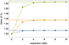 |
Fig. C.1. Value of the reduced skewness, S3, obtained at increasing order beyond the mean field. The mean field solution of the Rayleigh-Levy flights model, 3/2, is the same, whatever the index of the spectrum and the shape of the window function. The exact expression of S3 depends however slightly on the power law index and on the filter shape. They are indicated as dotted lines. One can see that corrections to the mean field solution converge very rapidly to the expected value. |
On the other hand the low density part turns out to be much more difficult to capture with a Gaussian filter. As illustrated in Figure 2, the density fields exhibit genuine large empty regions. This leads to a non-zero void probability density function for filters that have a compact support. However, for filters with extended radial tails, the probability of finding the filtered density to be exactly zero can only vanish, leading however to an excess of probability at low densities. This is illustrated in Figure 3. Unfortunately the mean field extensions as described here always lead to finite VPDF to all finite orders. This effect is illustrated in Fig. C.2, which also shows that the convergence of the PDF in the low density regions is slow. This is also illustrated at the level of the density PDF in Fig. 3. To conclude, i) the mean field solution is very efficient at predicting the high density regions but fails in the low density regions; ii) solutions beyond the mean field, Eqs. (C.4), can account for the behaviour of the PDFs in the low density regions, but the convergence is slow. Extension beyond the mean field in higher dimensions will be the topic of future work.
 |
Fig. C.2. Value of the void probability density function for ξ0 = 1 at increasing order beyond mean field solution. The expression of the VPDF depends both on the power law index and on the filter shape. For a Gaussian filter, we would expect the VPDF to identically vanish, since they have infinite spatial extensions, unlike filters with compact support. It makes the prediction derived from the mean field poor in the low density regime. |
Appendix D: Extrema and Euler densities
D.1. General formalism
The computation of extrema densities is relies on the knowledge of the joint PDF of the local density, its first and second order derivatives (Bardeen et al. 1986). The latter will be derived from the CGF of those quantities.
The number of relevant variables depend on the spatial dimension. To fix the notation we define ξ0, ξ1, and ξ2 as the variance of respectively the local density, the one-component density gradient and second derivatives:

assuming 〈ρ〉 = 1. We further note the consistency relations, which can be derived by integration via:
We then denote λρ, λi, and λij the conjugate variables to respectively ρ, ρ,i and ρ,ij (keeping in mind that ρ,ij and ρ,ji are identical).
In general the number density of extrema is given by Eq. (19). For instance, maxima are obtained when the integral is restricted to the regions where all eigenvalues are negative; minima when all eigenvalues are positive and in 2D, saddle points are obtained when the integral is restricted to the regions where the sign of the two eigenvalues is different. We finally note that Euler number densities are obtained with χextr.[ρ,ij] = 1. Its advantage is that it preserves the analytical structure of the operator making in general its derivation easier. Specifically, the formulae we obtain for the 1D and 2D cases are:
and a similar (if more involved) expression for the 3D case. For the Euler number density, taking advantage of its analyticity, it is possible to simply re-express it in terms of the CGF through inverse Laplace transforms. More precisely we have in 1D:

It shows that the Euler number density, unlike the extrema density in general, depends only on limited information from the joint CGF. For the 2D case, the calculations are similar but a bit more involved, as:
with a similar construction for the 3D case. Explicit derivation of the Euler number densities for the Rayleigh-Levy flight model are presented hereafter. We start with general consideration regarding the symmetry properties of both the CGF and the joint PDFs.
D.2. Spatial homogeneity & isotropy
In the cosmological context, density fields are statistically homogeneous and isotropic. For the hierarchical tree models, it is ensured by the fact that the two-point correlation function ξ2(x, x′) depends on |x − x′| only.
A number of properties follows. The first immediate one, for the 1D case, is that the expectation value of any gradient should vanish. That implies in particular that the expectation value of  vanishes, which implies Eq. (D.2). More generally a consequence of this invariance is that, for any integer p and q,
which in terms, after summing over p and q, implies
An alternative formulation at the level of the PDF reads
Integrating the second term of this equation over ρ,x up to ρ,x = 0 leads to the expression (D.3) of  so that the latter can eventually be written in terms of the joint probability of the density and its gradient as
It shows that the Euler number density does not depend actually on the way ρ,xx is correlated to the density and its gradient. This is not so for the extrema counts. This points to an interesting feature of Euler number density: it is significantly more insensitive to small scale fluctuations compared to other observables.
Unfortunately this simplification does not directly extend to higher dimensions. There are however a number of consistency relations that derive from statistical invariance under translation, parity change and rotation. They are
-
Translation invariance12: as in 1D, for any direction, i, we expect
-
Parity invariance: For dimensions above 2D, there are other combinations that vanish such that the expectation values of T,xU,y − T,yU,x (as can be shown by successive integrations by parts). For the 2D case, this is the transcription of parity invariance: the expectation of any rotational is expected to vanish. It implies that
and a similar equation after substitution y ↔ x. We note that the left-hand-side of this equation is the operator for the computation of the Hessian in 2D. It can be reduced to first order derivatives in λij. Contributions from joint cumulants between the density and its first and second order derivatives still however contribute to the Euler number density.
-
Rotation invariance: for a sake a completeness one can also derive the consequences of rotational invariance. We do it here for the 2D case: forcing λxρx + λyρy + λxxρxx + λxyρxy + λyyρyy to be rotation invariant, a rotation of the coordinate system by infinitesimal angle θ leads to
so that
with


![$$ \begin{aligned} \mathcal{R} \left[\varphi (\lambda _\rho ,\lambda _i,\lambda _{ij})\right]=0\,, \end{aligned} $$](/articles/aa/full_html/2024/09/aa49628-24/aa49628-24-eq166.gif)
We now turn by exploring scaling properties of the cumulants. Hierarchical models are by nature such that

In general, the cumulants of the product of powers of the local density, first and second order derivatives behave like  where s + t + u = n − 1, if the total power is n. We note that for dimensional reasons, if only the local density and first derivative is involved then
It is not possible to give rules when both density, first and second order derivatives are present. We can however note that

Finally we conjecture13 that the following scaling is expected,
It is indeed verified in the expressions derived below.
D.3. Derivation of join CGF in mean field limit
We now turn to writing the joint CGF for a given set of cells. The calculation is based on the mean field solution for a finite number of cells assumed to be infinitely close to one another; the derivatives are then obtained via finite differences. More precisely if two cells are at distance d, we then assume that the average correlation between the 2 cells, ξ(d), can be expanded in powers of d. Its expression can be derived using the correlation between the density and its gradient (again via integration by part)

so that
where the coefficients ξi are precisely those defined in Eq. (D.1).
The density gradient is then represented by a finite difference (ρi − ρj)/d is the two cells are at a distance, d. The conjugate variable associated with the density gradient, λx, would then contribute to both λi and λj with a weight, respectively, of 1/d and −1/d. In general we then build the multi-values CGF as a function of such quantities. To make the construction more explicit, we consider the 2D case. To do so we need at least 6 cells taken from a 3x3 grid. Each λα where α stands for ρ or its derivatives contribute through the following pattern
with a similar definition for Ly and Lyy. Defining the 3x3 matrix

the stationary equations become
where (Lλ)j is the jth element of the matrix Lλ. The CGF is then expressed as:
The result is a function of λα and of d, ξ0, ξ1 and ξ2 through the ξij dependence. The set of nine Eqs. (D.23) can be solved via MATHEMATICA, yielding a rather complex expression.
D.4. 1D Euler and extrema counts
In 1D, in the low d limit and for ξ0 = 0, the generating 1D function, φ1D(λρ, λx, λxx; 0, ξ1, ξ2), takes the remarkably simple form of:
Taking now advantage of the shifting relation (C.6), we can write, for a general ξ0,
![$$ \begin{aligned}&\varphi _{\rm 1D}(\lambda _{\rho },\lambda _{\rm x},\lambda _{\rm xx};\xi _{0},\xi _{1},\xi _{2})=\nonumber \\&\varphi _1\left[-\frac{2 \left(\xi _1 \lambda _x^2\!+\!\lambda _{\rho } \left(2\!-\!2 \xi _1 \lambda _{xx}\right)\!+\!\xi _2 \lambda _{xx}^2 \left(1\!-\!\xi _1 \lambda _{xx}\right)\right)}{\left(\xi _1 \lambda _{xx}\!-\! 1\right) \left(\xi _1 \lambda _{xx}\!+\!2\right)^2};\xi _0\right]. \end{aligned} $$](/articles/aa/full_html/2024/09/aa49628-24/aa49628-24-eq181.gif)
Equation (D.26) displays advantageous properties to complete the computation of number density of extrema. We indeed have:
which leads naturally to the change of variable
when computing the inverse Laplace transformation over λx, necessary for the joint PDF, Eq. (C.22). We are left with
We can further note that the dependence in λe in φ1D({λe,0,λxx};ξ0,ξ1,ξ2) now takes a very simple form
with
The integral over λe in Eq. (D.29) can then be done with the use of Eq. (C.24). It leads to the following expression (for the continuous, non singular, component)
where
We are now in position to compute the number densities of extrema of the various kinds. The Euler number density is obtained from the computation of Eq. (D.3) which can be obtained directly via the derivative of χ1D(ρ, λxx) defined in (D.34) with respect to λxx at position λxx = 0,
This finally leads to the following remarkable closed form expression for the 1D Euler number density of Levy flights
This is to be contrasted to the number density of Euler points in the Gaussian limit, which reads
which can also be obtained from more direct calculations (see, e.g. Bardeen et al. 1986). In general, it is of interest to be able to distinguish between the number counts of maxima and minima separately. This can be achieved via specific integration path in the complex plane as follows

where χ1D(ρ; λxx) is given by Eq. (D.34), while ϵ is a negative real constant for maxima and a positive real constant for minima14. This quadrature, together with its Euler counterpart, Eq. (D.36), is one of the key result of this paper.
D.5. 2D Euler and extrema counts
In 2D, it is best to re-organise the field variables. Indeed it is well known that while ρx and ρy form a vector field, κ = (ρxx + ρyy)/2 is a scalar field and γ1 = (ρxx − ρyy)/2 and γ2 = ρxy form a spin-2 field. It is then worth defining the CGF for those quantities and so to write it as a function of the conjugate variables of those components, that is, respectively λρ, λg1, λg2, λκ, λγ1, and λγ2. Furthermore, because the CGF must be rotationally invariant, it can be expressed in terms of the following scalar quantities:


Following the same steps as in 1D, using MATHEMATICA to compute the small d limit of the solution of the system of Eqs. (D.23), relying on the shifting relation (Eq. C.6) and re-expressing the resulting generating function in terms of the Λis, the final result for the generating function is expressed as:
![$$ \begin{aligned} \varphi _{\rm 2D}&(\lambda _{\rho },\Lambda _{i};\xi _{0},\xi _{1},\xi _{2})= \varphi _{1} \left[\frac{\lambda _{\rho }+\frac{1}{6} \left(2 \Lambda _1^2+\Lambda _3\right) \xi _2}{\left(\frac{\Lambda _1 \xi _1}{2}+1\right)^2}\right. \nonumber \\&- \left.\frac{\xi _1 \left(\Lambda _2 \left(\Lambda _1 \xi _1-2\right)-\Lambda _4 \xi _1\right)}{\left(\frac{\Lambda _1 \xi _1}{2}+1\right)^2 \left(\left(\Lambda _1^2-\Lambda _3\right) \xi _1^2-4 \Lambda _1 \xi _1+4\right)};\xi _{0}\right] . \end{aligned} $$](/articles/aa/full_html/2024/09/aa49628-24/aa49628-24-eq198.gif)
The calculation of the number density of extrema also follows the same steps as for the 1D case. We first remark that

with
which allows us to integrate over λg1 and λg2. This leads to the joint PDF,
Then, defining:
allows us to rewrite φ2D in Eq. (D.43) as:
Then we can carry out the integration over λe in Eq. (D.46) with the help of Eq. (C.24). This leads to the following expression for the joint PDF
where
that has to be integrated over λκ, λγ1 and λγ2. In the following we note γ the two component vector (γ1, γ2) and γn its norm,  . We also note
  . The resulting number density of Euler points follows through differentiation
which after some algebra yields the following final closed form for the 2D Euler count of Rayleigh-Levy flights
to be once again contrasted to the Gaussian counts
The computation of extrema number densities in 2D require us to distinguish the signs of the eigenvalues of the Hessian. In practice that means one should be able to split the integral over κ into 3 domains, κ < −γn, −γn < κ < γn and κ < γn. We first note that
which implies that
which leads to the following quadrature for the extrema counts
where ϵ is a negative real constant for maxima and a positive real constant for minima. This double quadrature, together with its Euler counterpart (D.53), is also one of the key result of this paper.
D.6. The 3D Euler and extrema counts
The 3D Euler and extrema counts can be similarly derived, although the calculation is somewhat more sophisticated. To sort out the results, we strive to take full advantage of the rotation invariance of the result and to be a bit more precise. The quantities, ρ, ρ,i and ρ,ij form respectively a tensor of rank 0, 1, and 2 with respect to coordinate changes  . Therefore we would like to derive the conjugate expression
  and
and  of the quantities obtained after a change of coordinates,
We should have
Replacing  by its expression in the right hand side of Eq. (D.58) ensures that

making clear that λi is a rank-1 co-tensor. This is not the case for λij as the sum in Eq. (D.58) excludes repeated symmetric quantities. We are then led to define
so that
It is then clear that  transforms as a rank-2 co-tensor. From the definition of Eq. (B.5), the CGF itself is also clearly invariant under rotations. We then expect it to depend on combinations of λi and
  that are scalar invariant. Eventually we found the expression of the CGF to depend on the following six invariant quantities
![$$ \begin{aligned} \Lambda _{3}&=\sum _{ij}\lambda ^R_{ij}\lambda ^R_{ij}\,,\quad \Lambda _{4}=\det \left[\lambda ^R_{ij}\right]\,,\end{aligned} $$](/articles/aa/full_html/2024/09/aa49628-24/aa49628-24-eq227.gif)
with
and

As in 1 and 2D, the integral over λi and λρ can be carried out explicitly. The computation of the Euler number density from Eq. (19) relies on the following rules for the integration over λij: det[ρ,ij] → det[∂/∂λij], identifying λij and λji. After some significant algebra, we eventually get
while the corresponding Gaussian limit is expressed as:
This completes our results regarding Euler number densities. We note that the 1D, 2D, and 3D results are strikingly similar. Their Gaussian limit is consistent with the results presented in (Codis et al. 2013), noting that ξ1 = ⟨|∇ρ|2⟩/3 and that the Euler characteristic and the genus differ by one integration.
Appendix E: Extrema correlation
The computation of the expected correlations of extrema is based on the derivation of the joint CGF for the density and its gradients at finite distance,

What makes its estimation complicated is that it depends not only on the distance, d, but also on the ratio of d with the smoothing scale, R. It is however possible to get a simple expression in the large separation limit. To carry out the calculation, we define ξ1(d) and ξ2(d) as, respectively, the first- and second-order derivative of the filtered densities at distance, d, and Taylor expand w.r.t. d as:
Using the same approach as before we can then derive joint CGF. An intermediate result is given by the expression of the following quantity
which in principle can be used to build cross matter-extrema correlations at any separation15. It is worth investigating this expression in the large separation limit. We assume that ξ0(d), ξ1(d) and ξ2(d) are all small quantities. We can further note that ξ2(d)ξ0 ≪ ξ0(d)ξ2 if d is much larger that the smoothing scale. We can then observe the following property in the large separation limit,

And more generally we can explicitly verify that
This is a property which is generic to MTM (Bernardeau 2022). More generally we expect that Eq. (34) holds. We note that the correction fully factorises in variables of each type.
In the large separation limit, the two-point number densities of critical points has correspondingly the following functional form:

where bcrit.(ρ) is defined by
![$$ \begin{aligned} b_{\rm crit.}(\rho )n_{\rm crit.}(\rho )\!=\!&\! \int \!\prod _{ij}{\mathrm{d}\rho _{,ij}} \mathrm{Sgn}\left[\rho _{,ij}\right] \det \left[\rho _{,ij}\right] \! P_b\!\left(\rho ,\rho _{,i}\!=\!0,\rho _{,ij}\right), \end{aligned} $$](/articles/aa/full_html/2024/09/aa49628-24/aa49628-24-eq239.gif)
where Sgn[ρ,ij] is given in Eq. (19) and we have
The calculation then follows the same articulation as before.
E.1. 1D bias asymptotic
For the 1D case we are led to
where
that derives from the use of Eqs. (C.24) and (C.25). It leads to the expression of the biased number density of Euler numbers and of maxima. We thus have
which gives the behaviour of the large scale bias factor.
E.2. 2D bias asymptotic
For the 2D case the corresponding form is:
which, after some algebra, leads to the bias factor
The expressions (D.34), (D.51), (E.10) and (E.12) are the central building blocks for the construction of the extrema correlations for the 1D and 2D cases.
Appendix F: Gaussian CGFs
The cumulant generating functions in their Gaussian limits the take the following form:
All Figures
|
Fig. 1. Two-point correlation function for the 1D Rayleigh-Levy flights (before smoothing). The predictions are for ℓ0 = 1. The solid lines are the exact shapes derived from Eq. (5) exhibiting a clear exclusion zone for r < ℓ0. The dashed is the large scale asymptotic form. it can be observed that the exact solution converges very rapidly to the asymptotic form. |
| In the text | |
|
Fig. 2. Example of a 2D density field derived from a 2D levy flight. Parameters of the flight are α = 1., ℓ0 = 0.012 pixel size with ten points per pixel. The sample has periodic boundary conditions with 2002 pixels. The initial discrete (point) field has been convolved with a Gaussian window function of width of 2 (in pixel size) in each direction. The resulting variance as measured in the sample is 1.56. On the plot, the contour lines are log-spaced, from density of about 0.2–7. The deep blue regions correspond to empty regions. |
| In the text | |
|
Fig. 3. Comparisons of measured density PDF from a set of 1D Rayleigh-Levy flights whose characteristics are given in the text, grey points, compared to different levels of theoretical predictions. The blue dotted line is the mean field approximation. The other lines correspond to different level of approximation, up to sixth order in an expansion in Hermite Polynomials. |
| In the text | |
|
Fig. 4. Mean field predictions for extrema counts and comparison with 1D numerical Levy flight for two different indices as labelled. See text for details on the measurements. We note the Euler number density is negative on the low density branch as the number density of minima exceeds the number density of maxima. The agreement between theory and measurements is remarkable. |
| In the text | |
|
Fig. 5. Mean field prediction for extrema counts for 2D fields. The plots are for ξ0 = 1 and γ = 0.45. |
| In the text | |
|
Fig. 6. Theoretical prediction for the bias function of 1D extrema, of Euler points and that of the local density, Eq. (32), and its corresponding large scale limit (dashed line) as given by Eq. (33). As expected, the maxima and Euler points have the same bias at a high density, this is also the bias of the density field itself: high density critical points are likely to be maxima of the fields and their correlation properties is to a large extent determine by density bias. |
| In the text | |
|
Fig. 7. Theoretical prediction for the bias function of 2D extrema, saddle points, Euler points and that of the local density (for which the predictions is the same as in 1D). Similar conclusions can be drawn from the 1D case. |
| In the text | |
|
Fig. 8. Correlation function of the thresholded density regions and comparisons with predictions. The black solid line is the measured matter correlation function. The dashed lines are the prediction correlation amplitudes for thresholded regions derived from their large-scale limit. They have been computed after applying bias factors b#(> ρs)2 to ξ0(d) as measured in the simulation. |
| In the text | |
|
Fig. 9. Same as previous figure for the thresholded maxima. Open symbols correspond to negative values. We see a sharp transition between the large-scale behaviour – well predicted by the theory – and the small-scale behaviour. Note: the plateau at small scale corresponds to ξmax(d) = − 1, meaning that peaks generate an exclusion zone in their vicinity. |
| In the text | |
|
Fig. 10. Same as previous figure for the thresholded minima. We note that the minima are, as expected, more clustered than maxima for a given threshold value. We still observe a transition towards the small scale to ξmaxima(d) = − 1. We note that this measure is too noisy for a threshold ρs > 4. (not shown here). |
| In the text | |
|
Fig. 11. Same as previous figure for the thresholded Euler number densities. We still observe a transition towards the small scale. We note that here ξEuler(d) < − 1 showing that minima and maxima tend to be correlated at small distance (as confirmed in the next plot). Note: this measure is quite noisy as the Euler number density vanishes for low thresholded values and the threshold ρs > 0.5 is not shown. |
| In the text | |
|
Fig. 12. Cross-correlation between minima and maxima with the same threshold. The prediction is obtained here by multiplying ξ0(d) as measured in the simulation by bmin(> ρs)bmax(> ρs). We note a large positive correlation for scales that are of the order of the smoothing scale. |
| In the text | |
|
Fig. C.1. Value of the reduced skewness, S3, obtained at increasing order beyond the mean field. The mean field solution of the Rayleigh-Levy flights model, 3/2, is the same, whatever the index of the spectrum and the shape of the window function. The exact expression of S3 depends however slightly on the power law index and on the filter shape. They are indicated as dotted lines. One can see that corrections to the mean field solution converge very rapidly to the expected value. |
| In the text | |
|
Fig. C.2. Value of the void probability density function for ξ0 = 1 at increasing order beyond mean field solution. The expression of the VPDF depends both on the power law index and on the filter shape. For a Gaussian filter, we would expect the VPDF to identically vanish, since they have infinite spatial extensions, unlike filters with compact support. It makes the prediction derived from the mean field poor in the low density regime. |
| In the text | |
Current usage metrics show cumulative count of Article Views (full-text article views including HTML views, PDF and ePub downloads, according to the available data) and Abstracts Views on Vision4Press platform.
Data correspond to usage on the plateform after 2015. The current usage metrics is available 48-96 hours after online publication and is updated daily on week days.
Initial download of the metrics may take a while.