© The Authors 2025

1. Introduction

The coronal heating problem has been a topic of research for several decades and has still not been fully solved. Various processes have been proposed as potential contributions to the heating of the coronal plasma. These processes can be classified into two categories: direct current (DC) heating, and alternating current (AC) heating. The former relies on the process of magnetic reconnection and on the creation of current sheets as a result of the intertwining of magnetic field lines, such that Ohmic dissipation can convert magnetic energy into heat. The latter relies on magnetohydrodynamic (MHD) waves that convey energy either from the lower layers of the atmosphere or from the location of an impulsive event. This energy is then released into the background plasma via dissipation mechanisms such as viscous or Ohmic diffusion. Some of the wave-related processes that received considerable attention are phase mixing (Heyvaerts & Priest 1983; Soler et al. 2013), during which Alfvén or slow waves propagate on neighboring field lines at slightly different speeds and gradually drift out of phase, such that large gradients develop and dissipation becomes efficient. Another process is resonant absorption (Hollweg & Yang 1988; Sakurai et al. 1991; Goossens et al. 2002), which is a closely related process in which the energy of a wave is transferred to local Alfvén or slow-mode oscillations in isolated magnetic surfaces until large cross-surface gradients develop and permit dissipation to become efficient.

Null points are particular locations in the solar magnetic field in which the magnetic field and hence the Alfvén speed vanishes. X-type null points (or X-points) are a particular form of a null point in the form of the letter X and are known to be present in the coronal magnetic field, where they play a role in the local heating of the coronal plasma. They can indeed collapse and form a current sheet in the process, from which the magnetic energy can be released in the form of heat through magnetic reconnection. The connection between waves and X-point heating was discussed, for example, by Longcope & Priest (2007). Several studies have investigated the damping rate of Alfvén and magnetosonic waves that evolve near an X-point in an effort to determine the associated heating rate (Craig & McClymont 1991; Craig & Watson 1992; Hassam 1992; Ofman et al. 1993; Hassam & Lambert 1996). McLaughlin & Hood (2004) showed for a pressureless plasma (β = 0) that fast magnetosonic waves wrap around the X-point, where the current rapidly accumulates and the energy of the waves is dissipated, whereas Alfvén waves dissipate their energy along the separatrixes. However, Craig & Watson (1992) found that the inclusion of a nonzero plasma pressure hampers the rapid current build-up at the null point. Some authors have also investigated nonlinear effects. McLaughlin et al. (2009) extended the model of Craig & McClymont (1991) to include plasma pressure and nonlinearity. They found that fast and slow magnetosonic waves form shocks that greatly alter the X-point structure, which finally collapses into a current sheet. Gruszecki et al. (2011) investigated shock formation due to nonlinear fast magnetosonic waves that propagate toward an X-point. They concluded that only smooth and low-amplitude pulses can reach the vicinity of the X-point, where they create spikes in the current density and trigger magnetic reconnection. Prokopyszyn et al. (2019) studied nonlinear Alfvén wave phase mixing numerically and found that the nonlinear effects reduce the energy that enters the domain, but they do not affect the damping of the waves strongly. The nonlinearity also has the effect of forming density structures that change the local Alfvén speed and displace the location of the resonance. Oscillations around X-points can furthermore be important in the generation of quasi-periodic pulsations in solar and stellar flares (Van Doorsselaere et al. 2016). Santamaria & Van Doorsselaere (2018) performed two-dimensional numerical simulations of wave propagation in the vicinity of a null point located in the corona to demonstrate why waves are generated at high frequencies. They showed that the frequency depends on the physical parameters of the atmosphere in the corona and does not depend on the driving strength. Therefore, the null point behaves as a resonant cavity that produces waves at specific frequencies depending on the background equilibrium model. They also demonstrated that the high-frequency wave train produced at null points is not necessarily the result of the interaction of shock waves and null points, but can be the outcome of the interaction between null points and fast acoustic waves.

In this paper, the focus lies on the Alfvén continuum eigenmodes around an X-point with a circular boundary and a guide field out of the X-point plane. We derive the equations governing the Alfvén continuum modes and solve them numerically, except for the special case without a guide field, for which we find analytical solutions. The Alfvén continuum modes are important for phase mixing and resonant absorption of MHD waves as they form a complete orthogonal set and can thus be used to describe any perturbation through a linear combination of these waves. This is important for determining the conditions for resonant absorption to occur, for example, which could form a study that follows up on the results presented in this paper.

2. Model

We derived the Alfvén continuum modes around an X-point with a guide field. The ideal MHD equations were linearized, so that the thermal pressure p, plasma velocity v, mass density ρ, and magnetic field B were decomposed into an equilibrium part (denoted by the subscript 0) and a small perturbed part (denoted by the subscript 1). We assumed that there is no background flow, so v₀ = 0. The equilibrium density ρ₀ was assumed to be constant. The equilibrium magnetic field B₀ consists of the sum of a field in the form of a 2D X-point denoted by B_0p and a constant guide field denoted by B_0t,

$$\begin{array}{c}\hfill {\mathit{B}}_0={\mathit{B}}_{0p}+{\mathit{B}}_{0t}.\end{array}$$(1)

In Cartesian coordinates, the equilibrium X-point field and guide field are given by the following expressions:

$$\begin{array}{cc}\hfill {\mathit{B}}_{0p}& {\displaystyle =\frac{B_R}{L_R}\left(\begin{array}{c}z\\ 0\\ x\end{array}\right),}\hfill \end{array}$$(2)

$$\begin{array}{cc}\hfill {\mathit{B}}_{0t}& =\left(\begin{array}{c}0\\ B_{0y}\\ 0\end{array}\right),\hfill \end{array}$$(3)

where B_R and L_R are reference values for the magnetic field strength and length, respectively, and B_0y is a constant. The equilibrium thermal pressure p₀ was allowed to vary in x and z as well. The perturbed quantities can be Fourier-analyzed in the y-coordinate and in time t: $f_1={\stackrel{\sim }{f}}_1(x,z)exp\{i(k_{\mathit{y}}\mathit{y}-\omega t)\}$ for the perturbed quantities p₁, v_1r, v_1φ, v_1z, ρ₁, B_1r, B_1φ, and B_1z. Thus, the ignorable coordinate along which the constant guide field lies is y, whereas the equilibrium 2D X-point field lies in the xz-plane.

The X-point component can be written with a flux function ψ as follows:

$$\begin{array}{c}\hfill {\mathit{B}}_{0p}=-\mathrm{\nabla }\psi (x,z)\times {\mathbf{1}}_y=\left(\begin{array}{c}\frac{\partial \psi }{\partial z}\\ 0\\ -\frac{\partial \psi }{\partial x}\end{array}\right).\end{array}$$(4)

The flux function ψ can then be calculated to be

$$\begin{array}{c}\hfill {\displaystyle \psi (x,z)=\frac{B_R}{L_R}\frac{z^2-x^2}{2}.}\end{array}$$(5)

The contour lines given by ψ(x, z) = C (with C a constant) are then the flux lines of the X-point magnetic field. In addition to ψ(x, z) and y, a third coordinate along the X-point field can be defined: χ. Then, (ψ, χ, y) forms a right-handed system of locally orthogonal coordinates, which are called flux coordinates. Since ψ(x, z) lies in the xz-plane and ∇χ ⋅ ∇ψ = 0 by definition, the following must hold:

$$\begin{array}{c}\hfill \mathrm{\nabla }\chi =\lambda (x,z){\mathit{B}}_{0p},\end{array}$$(6)

with λ a freely chosen function.

The simplest choice, if feasible, would be λ(x, z) = 1/||B_0p||. In this case, ∇χ = 1_B0p (where 1_B0p is defined as B_0p/||B_0p||), and the flux coordinate χ would then be the arc length along an X-point magnetic field line. We have

$$\begin{array}{c}\hfill {\displaystyle {\left(\mathrm{d}s\right)}^2=\frac{1}{B_{0\chi }^2}{\left(\mathrm{d}\psi \right)}^2+J^2{B}_{0\chi }^2{\left(\mathrm{d}\chi \right)}^2+{\left(\mathrm{d}y\right)}^2}\end{array}$$(7)

for the elementary length ds in the local system of orthogonal flux coordinates, with B_0χ = ||B_0p|| and $J=\frac{1}{B_{0\chi }||\mathrm{\nabla }\chi ||}$ the Jacobian of the transformation of the Cartesian coordinate system into the flux coordinate system (Kaneko et al. 2015). At constant ψ and y, Eq. (7) then yields ds = dχ, with s the arc length along an X-point magnetic field line.

However, 1_B0p is not a potential field, which means that we cannot find a χ that satisfies ∇χ = 1_B0p. We thus took λ(x, z) = 1 for all (x, z). This entailed that ∇χ = B_0p, and in this case, we found the solution

$$\begin{array}{c}\hfill {\displaystyle \chi (x,z)=\frac{B_R}{L_R}xz.}\end{array}$$(8)

The advantage is that now a relatively simple expression for χ is found. However, the disadvantage is that the flux coordinate χ is not the arc length s along an X-point magnetic field line. This must be taken into account when we seek the profiles of the Alfvén continuum eigenfunctions along magnetic field lines.

Figure 1 shows lines of constant ψ(x, z) (left panel) and constant χ(x, z) (right panel). The Cartesian coordinates x and z can be written as a function of the new coordinate system as follows:

$$\begin{array}{cc}& x=\{\begin{array}{cc}{\displaystyle \frac{\chi }{\sqrt{\psi +\sqrt{{\chi }^2+{\psi }^2}}}\sqrt{\frac{L_R}{B_R}}}\hfill & \text{if}z\ge 0\hfill \\ {\displaystyle -\frac{\chi }{\sqrt{\psi +\sqrt{{\chi }^2+{\psi }^2}}}\sqrt{\frac{L_R}{B_R}}}\hfill & \text{if}z<0\hfill \end{array},\hfill \end{array}$$(9)

$$\begin{array}{cc}& z=\{\begin{array}{cc}{\displaystyle \sqrt{\psi +\sqrt{{\chi }^2+{\psi }^2}}\sqrt{\frac{L_R}{B_R}}}\hfill & \text{if}z\ge 0\hfill \\ {\displaystyle -\sqrt{\psi +\sqrt{{\chi }^2+{\psi }^2}}\sqrt{\frac{L_R}{B_R}}}\hfill & \text{if}z<0\hfill \end{array}.\hfill \end{array}$$(10)

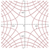Fig. 1. Lines of constant flux coordinates ψ and χ. The solid lines show regions of constant ψ(x, z). These are the field lines of B0p. The dashed lines show regions of constant χ(x, z).

For later use, it should also be noted that the Jacobian of the transformation from Cartesian to flux coordinates is given by

$$\begin{array}{c}\hfill {\displaystyle J=\frac{1}{2\sqrt{{\chi }^2+{\psi }^2}}\frac{L_R}{B_R}.}\end{array}$$(11)

Furthermore, the strength of the X-point magnetic field can be written in flux coordinates as

$$\begin{array}{c}\hfill {\displaystyle B_{0\chi }=\sqrt{2}{({\chi }^2+{\psi }^2)}^{1/4}\sqrt{\frac{B_R}{L_R}},}\end{array}$$(12)

from which it follows that

$$\begin{array}{c}\hfill {\displaystyle \frac{\mathrm{d}{B}_{0\chi }}{d\chi }=\frac{2\chi }{B_{0\chi }^3}\frac{B_R^2}{L_R^2}}\end{array}$$(13)

and

$$\begin{array}{c}\hfill {\displaystyle J=\frac{1}{B_{0\chi }^2}.}\end{array}$$(14)

Perturbed physical quantities f₁ are henceforth written as functions of the flux coordinates (ψ, χ, y) instead of the Cartesian coordinates (x, y, z),

$$\begin{array}{c}\hfill f_1={\tilde{f}}_1(\psi ,\chi )exp\left\{i(k_{y}y-\omega t)\right\}.\end{array}$$(15)

3. Governing equations

The linearized ideal MHD equations read (Kadomtsev 1966)

$$\begin{array}{c}\hfill \rho \frac{{\partial }^2\mathit{\xi }}{\partial t^2}=-\mathrm{\nabla }{p}_1-\frac{1}{{\mu }_0}({\mathit{B}}_1\times (\mathrm{\nabla }\times {\mathit{B}}_0)+{\mathit{B}}_0\times (\mathrm{\nabla }\times {\mathit{B}}_1)),\end{array}$$(16a)

$$\begin{array}{c}\hfill p_1=-\mathit{\xi }·\mathrm{\nabla }{p}_0-\gamma p_0\mathrm{\nabla }·\mathit{\xi },\end{array}$$(16b)

$$\begin{array}{c}\hfill {\mathit{B}}_1=-\mathrm{\nabla }\times ({\mathit{B}}_0\times \mathit{\xi }),\end{array}$$(16c)

where ρ, p₀, and B₀ are the background density, kinetic pressure, and magnetic field, respectively. Furthermore, ξ is the Lagrangian displacement vector, and p₁ and B₁ are the Eulerian perturbations of the pressure and magnetic field, respectively. Here, γ is the ratio of specific heats, and μ₀ is the permeability of free space. Goossens et al. (1985) derived Equations (16a–16c) that determine the continuous spectrum for a general 2D magnetostatic equilibrium in the flux coordinate system (χ, ψ, y), which is left-handed with our specific choice of χ and ψ. However, we find that their equations remain unchanged for our right-handed flux coordinate system (ψ, χ, y). The equations that govern the continuous spectrum are obtained by taking the limit $\frac{\partial }{\partial \psi }\to \infty$. The following set of equations for continuum modes is then obtained:

$$\begin{array}{cc}& \frac{\partial P_1}{\partial \psi }+\frac{2}{{\mu }_{0}J}\frac{\partial }{\partial \psi }\left(J{B}_{0\chi }\right)B_{1\chi }=0,\hfill \end{array}$$(17)

$$\begin{array}{cc}& {\displaystyle {\rho }_0{\omega }^2{\xi }_{\chi }+\frac{1}{{\mu }_0{B}_{0\chi }}F({\mathit{B}}_0·{\mathit{B}}_1)-\frac{B_{0y}}{{\mu }_0{B}_{0\chi }}F\left(B_{1y}\right)=0,}\hfill \end{array}$$(18)

$$\begin{array}{cc}& {\displaystyle {\rho }_0{\omega }^2{\xi }_y+\frac{1}{{\mu }_0}F\left(B_{1y}\right)=0,}\hfill \end{array}$$(19)

$$\begin{array}{cc}& F\left({\displaystyle \frac{{\xi }_{\chi }}{B_{0\chi }}}\right)+\frac{1}{\gamma p_{0}J}\frac{\partial p_0}{\partial \chi }\frac{{\xi }_{\chi }}{B_{0\chi }}-\frac{B_{1\chi }}{B_{0\chi }}-\frac{B_{0\chi }{B}_{1\chi }+B_{0y}{B}_{1y}}{{\mu }_0\gamma p_0}=0,\hfill \end{array}$$(20)

$$\begin{array}{cc}& B_{1\psi }=0,\hfill \end{array}$$(21)

$$\begin{array}{cc}& \frac{\partial X}{\partial \psi }+\frac{B_{1\chi }}{B_{0\chi }}+i{k}_{y}Q=0,\hfill \end{array}$$(22)

$$\begin{array}{cc}& F\left(Q\right)-\left({\displaystyle B_{1y}-\frac{B_{0y}}{B_{0\chi }}{B}_{1\chi }}\right)=0,\hfill \end{array}$$(23)

where $P_1=p_1+\frac{{\mathit{B}}_0·{\mathit{B}}_1}{{\mu }_0}$ is the perturbed total pressure. ξ_ψ, ξ_χ, and ξ_y are the Lagrangian displacement components along the ψ, χ, and y axes. $F=\frac{1}{J}\frac{\partial }{\partial \chi }+i{k}_{\mathit{y}}{B}_{0\mathit{y}}$ is an operator, $Q={\xi }_{\mathit{y}}-\frac{B_{0\mathit{y}}}{B_{0\chi }}{\xi }_{\chi }$ and X = B_0χξ_ψ. Because $\frac{\partial }{\partial \psi }\to \infty$, we neglected Q and $\frac{\partial Q}{\partial \chi }$ was neglected compared to p for any perturbed quantity $\frac{\partial Q}{\partial \psi }$ that was differentiated with respect to ψ.

Out of Equations (18)–(20) and (23), the following two coupled second-order ordinary differential equations for ξ_χ and ξ_y can be derived (see Appendix A):

$$\begin{array}{cc}& {\displaystyle {\rho }_0{\omega }^2{\xi }_y+\frac{1}{{\mu }_0}F[\frac{{\mu }_0\gamma p_0{B}_{0y}}{B_{0y}^2+{\mu }_0\gamma p_0+B_{0\chi }^2}F\left(\frac{{\xi }_{\chi }}{B_{0\chi }}\right)}\hfill \\ \hfill & +\frac{{\mu }_0{B}_{0\chi }{B}_{0y}}{B_{0y}^2+{\mu }_0\gamma p_0+B_{0\chi }^2}\frac{\partial p}{\partial \chi }{\xi }_{\chi }+\frac{{\mu }_0\gamma p_0+B_{0\chi }^2}{B_{0y}^2+{\mu }_0\gamma p_0+B_{0\chi }^2}F(Q)]=0,\hfill \end{array}$$(24)

$$\begin{array}{cc}& {\displaystyle {\rho }_0{\omega }^2{\xi }_{\chi }+\frac{1}{{\mu }_0{B}_{0\chi }}F[\frac{{\mu }_0\gamma p_0{B}_{0\chi }^2}{B_{0y}^2+{\mu }_0\gamma p_0+B_{0\chi }^2}F\left(\frac{{\xi }_{\chi }}{B_{0\chi }}\right)}\hfill \\ \hfill & +\frac{{\mu }_0{B}_{0\chi }^3}{B_{0y}^2+{\mu }_0\gamma p_0+B_{0\chi }^2}\frac{\partial p_0}{\partial \chi }{\xi }_{\chi }-\frac{B_{0\chi }^2{B}_{0y}}{B_{0y}^2+{\mu }_0\gamma p_0+B_{0\chi }^2}F(Q)]=0.\hfill \end{array}$$(25)

3.1. Normalizing variables

Before we proceeded, all the variables were normalized. This allowed us to disregard dimensions and thus drop constants such as L_R and B_R in the equations. This simplifies the notation. The next section presents solutions to these equations under some specific simplifying conditions, and where the boundary of the system is an infinite straight cylinder with a circular cross section. The X-point magnetic field thus has a circle for a boundary as it lies in planes that are parallel to the xz-plane. We took the reference length L_R as the radius of this circle. The reference magnetic field strength B_R is the strength of the X-point field on the circle (as can be calculated from Eq. (2)). The reference density ρ_R was taken equal to ρ₀, the background density. The reference magnetic permeability μ_R was also taken to be μ₀. This entails that the reference speed v_R is the Alfvén speed on the boundary circle, $B_R/\sqrt{{\mu }_R{\rho }_R}$, and the reference frequency is ${\omega }_R={\mathit{v}}_R/L_R=B_R/(\sqrt{{\mu }_R{\rho }_R}{L}_R)$. The physical quantities f were rewritten as f_Rf_*, with f_R the reference value of f, and f_* the dimensionless value. We then had

$$\begin{array}{cc}& {\left(\begin{array}{ccc}x& y& z\end{array}\right)}^t=L_R{\left(\begin{array}{ccc}{x}_{\ast }& y_{\ast }& z_{\ast }\end{array}\right)}^t,\hfill \end{array}$$(26)

$$\begin{array}{cc}& {\left(\begin{array}{ccc}{\xi }_{\psi }& {\xi }_{\chi }& {\xi }_y\end{array}\right)}^t=L_R{\left(\begin{array}{ccc}{\xi }_{\psi ,\ast }& {\xi }_{\chi ,\ast }& {\xi }_{y,\ast }\end{array}\right)}^t,\hfill \end{array}$$(27)

$$\begin{array}{cc}& {\displaystyle {\mathit{B}}_p=\frac{B_R}{L_R}{\left(\begin{array}{ccc}z& 0& x\end{array}\right)}^t=B_R{\left(\begin{array}{ccc}{z}_{\ast }& 0& x_{\ast }\end{array}\right)}^t,}\hfill \end{array}$$(28)

$$\begin{array}{cc}& {\mathit{B}}_t={\left(\begin{array}{ccc}0& B_{0y}& 0\end{array}\right)}^t=B_R{\left(\begin{array}{ccc}0& B_{0y,\ast }& 0\end{array}\right)}^t,\hfill \end{array}$$(29)

$$\begin{array}{cc}& \psi (x,z)=B_R{L}_R{\psi }_{\ast }(x_{\ast },z_{\ast }),\hfill \end{array}$$(30)

$$\begin{array}{cc}& \chi (x,z)=B_R{L}_R{\chi }_{\ast }(x_{\ast },z_{\ast }),\hfill \end{array}$$(31)

$$\begin{array}{cc}& {\displaystyle k_y=\frac{1}{L_R}{k}_{y,\ast },}\hfill \end{array}$$(32)

$$\begin{array}{cc}& {\displaystyle p=\frac{B_R^2}{{\mu }_R}{p}_{\ast },}\hfill \end{array}$$(33)

$$\begin{array}{cc}& {\rho }_0={\rho }_R,\hfill \end{array}$$(34)

$$\begin{array}{cc}& {\mu }_0={\mu }_R.\hfill \end{array}$$(35)

Inserting expressions (26)–(35) into Eqs. (24) and (25) yields the following equations with quantities in dimensionless form (dropping the subscript for simplicity):

$$\begin{array}{cc}& {\displaystyle {\omega }^2{\xi }_y+F[\frac{\gamma p_0{B}_{0y}}{B_{0y}^2+\gamma p_0+B_{0\chi }^2}F\left(\frac{{\xi }_{\chi }}{B_{0\chi }}\right)}\hfill \\ \hfill & +\frac{B_{0\chi }{B}_{0y}\gamma }{B_{0y}^2+\gamma p_0+B_{0\chi }^2}\frac{\partial p_0}{\partial \chi }{\xi }_{\chi }+\frac{\gamma p_0+B_{0\chi }^2}{B_{0y}^2+\gamma p_0+B_{0\chi }^2}F(Q)]=0,\hfill \end{array}$$(36)

$$\begin{array}{cc}& {\displaystyle {\omega }^2{\xi }_{\chi }+\frac{1}{B_{0\chi }}F[\frac{\gamma p_0{B}_{0\chi }^2}{B_{0y}^2+\gamma p_0+B_{0\chi }^2}F\left(\frac{{\xi }_{\chi }}{B_{0\chi }}\right)}\hfill \\ \hfill & +\frac{B_{0\chi }^3}{B_{0y}^2+\gamma p_0+B_{0\chi }^2}\frac{\partial p_0}{\partial \chi }{\xi }_{\chi }-\frac{B_{0\chi }^2{B}_{0y}}{B_{0y}^2+\gamma p_0+B_{0\chi }^2}F(Q)]=0.\hfill \end{array}$$(37)

3.2. X-point without a guide field

In the case of a 2D X-point equilibrium without a guide field field (i.e., B_0y = 0), Eqs. (36) and (37) simplify and become decoupled,

$$\begin{array}{c}\hfill {\omega }^2{\xi }_y+F(F({\xi }_y))=0,\end{array}$$(38)

$$\begin{array}{c}\hfill {\displaystyle {\omega }^2{\xi }_{\chi }+\frac{1}{B_{0\chi }}F[\frac{\gamma p_0{B}_{0\chi }^2}{\gamma p_0+B_{0\chi }^2}F\left(\frac{{\xi }_{\chi }}{B_{0\chi }}\right)+\frac{B_{0\chi }^3}{\gamma p_0+B_{0\chi }^2}\frac{\partial p_0}{\partial \chi }{\xi }_{\chi }]=0,}\end{array}$$(39)

with now $F=\frac{1}{J}\frac{\partial }{\partial \chi }$. The solutions, with the amplitude of Lagrangian displacements, ${\stackrel{\sim }{\xi }}_{\mathit{y}}(\chi )$ and ${\stackrel{\sim }{\xi }}_{\chi }(\chi )$ of these two ordinary differential equations in χ are the regular parts of the respective full solutions ξ_y and ξ_χ and represent Alfvén and slow continuum waves, respectively. They show the dependence of ξ_y and ξ_χ on χ on a particular flux surface |ψ| = ψ₀. We drop the tilde from now on for clarity in the notation.

With the help of Eqs. (12)–(14), we found that $B_{0\chi ,\ast }=1/\sqrt{J}=\sqrt{2}{({\chi }_{*}^2+{\psi }_{*}^2)}^{1/4}$. Hence, Eq. (38) can be rewritten as

$$\begin{array}{c}\hfill 4({\chi }^2+{\psi }^2)\sqrt{2}\frac{\partial {\xi }_y}{\partial \chi }+4\chi \frac{\partial {\xi }_y}{\partial \chi }+{\omega }^2{\xi }_y=0.\end{array}$$(40)

It has the following analytical solution, found using the Maple software:

$$\begin{array}{c}\hfill {\xi }_y(\chi )=C_{1}cos\left(\lambda \omega \right)+C_{2}sin\left(\lambda \omega \right),\end{array}$$(41)

with $\lambda =ln\left(\sqrt{\chi +\sqrt{{\chi }^2+{\psi }^2}}\right)=ln(x+z)$. Equation (39), in contrast, does not seem to have an analytical solution. Because we are interested in the Alfvén continuum, its numerical solution was not considered here.

The solution (41) is given as a function of the dimensionless coordinate χ. However, χ is not the arc length coordinate along the X-point field lines. From Eqs. (7), (12) and (14), we find that at constant ψ and y,

$$\begin{array}{c}\hfill \frac{\mathrm{d}\chi }{\mathrm{d}s}=\sqrt{2}{({\chi }^2+{\psi }^2)}^{1/4}.\end{array}$$(42)

Hence, dχ is only equal to the elementary length along the X-point field lines at the unit circle, where the right-hand side of Eq. (42) is equal to 1. With s denoting the arc length along the X-point field lines from now on, we thus need to find the solution χ(s) of Eq. (42) in order to express the solution (41) for ξ_y as a function of s. However, Eq. (42) does not seem to have a closed-form analytical solution, and it therefore needed to be solved numerically. We considered a boundary to the X-point system: A circle of radius equal to L_R = L/R, centered in the middle of the X-point was considered here. The system is thus made of hyperbolic flux lines inside a circle (see Fig. 2). The Alfvén continuum frequencies ω on a particular flux surface can then be found by imposing the boundary conditions that ξ_y vanishes at the circle. For each field line, there is a countably infinite number of intervals of continuum frequencies, each of which corresponds to a tone (Goossens et al. 1985; Kaneko et al. 2015).

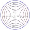Fig. 2. Studied system composed of an X-point configuration inside a circle and with a constant guide field perpendicular to it.

The circle with a normalized radius equal to 1 in the xz-plane is defined in Cartesian coordinates as x² + z² = 1. Its expression in terms of flux coordinates can be found with the help of Eqs. (9) and (10),

$$\begin{array}{c}\hfill {\displaystyle \sqrt{{\chi }^2+{\psi }^2}=\frac{1}{2}.}\end{array}$$(43)

Then, from Eq. (43), χ can be expressed as a function of ψ on the circle,

$$\begin{array}{c}\hfill {\displaystyle \chi =\pm \frac{\sqrt{1-4{\psi }^2}}{2}.}\end{array}$$(44)

This gives the expressions of χ at the two boundaries on a specific flux line |ψ| = ψ₀ inside the circle. It can also be checked that

$$\begin{array}{c}\hfill |\psi |,|\chi |<0.5\end{array}$$(45)

holds inside the circle. The value |χ| = 0.5 is achieved on the four intersections of the separatrixes z = ±x with the circle. Similarly, the value |ψ| = 0.5 is achieved on the four intersections of the x and z-axes with the circle and represents hyperbolas tangent to the circle in the points (1, 0), ( − 1, 0), (0, 1), and (0, −1) and located fully outside of it. Furthermore, χ = 0 corresponds to the x- and z -axes, whereas ψ = 0 corresponds to the separatrixes z = ±x forming the X shape. In Fig. 3, two example flux lines are shown. We worked in 3D, and therefore, |ψ| = ψ₀ for a certain ψ₀ is a flux surface of which we only see the projection onto the xz-plane in Figs. 2 and 3.

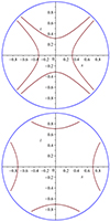Fig. 3. Flux lines (red) corresponding to |ψ| = 0.05 (left) and |ψ| = 0.25 (right), within the boundary circle (blue).

In order to plot an eigenfunction on a particular field line as a function of the arc length s, we first need to know the value of s at the boundaries given by Eq. (44). As on a particular flux line χ is only dependent on s, we find from Eq. (42) that

$$\begin{array}{c}\hfill {\displaystyle \frac{\mathit{ds}}{d\chi }=\frac{1}{\sqrt{2}{({\chi }^2+{\psi }^2)}^{1/4}}.}\end{array}$$(46)

For each particular value of ψ, we first solved Eq. (46) subject to s(0) = 0 numerically, so that we could determine the values $s(-\frac{\sqrt{1-4{\psi }^2}}{2})$ and $s\left(\frac{\sqrt{1-4{\psi }^2}}{2}\right)$ of s on the boundary of the given flux line. Next, we solved Eq. (42) numerically and inserted the values of χ in terms of s between the two boundaries into the formula (41). In this way, we obtained a plot of ξ_y as a function of s. The profiles of ξ_y as a function of s on the flux lines of Fig. 3 are shown as solid lines in Fig. 4 and Fig. 5 for the fundamental tone and the first overtone, respectively.

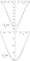Fig. 4. Perpendicular displacement (ξ⊥) of the fundamental tone of the Alfvén continuum mode as a function of the X-point magnetic field arc length (s) on the flux lines |ψ| = 0.05 (left) and |ψ| = 0.25 (right) for B0y = 0 (solid line), B0y = 2 (dashed line), B0y = 10 (dash-dotted line), and B0y = 100 (dotted line).

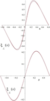Fig. 5. Perpendicular displacement (ξ⊥) of the first overtone of the Alfvén continuum mode as a function of the X-point magnetic field arc length (s) on the flux lines |ψ| = 0.05 (left) and |ψ| = 0.25 (right), for B0y = 0 (solid line), B0y = 2 (dashed line), B0y = 10 (dash-dotted line), and B0y = 100 (dotted line).

The frequencies of the Alfvén coninuum modes are found by imposing ξ_y(χ) = 0 at the two boundaries (44) and demanding that the system has nontrivial solutions in C₁, C₂. This yields the following continuum frequencies:

$$\begin{array}{c}\hfill {\displaystyle \omega =\frac{k\pi }{ln\left(\sqrt{\frac{1+\sqrt{1-4{\psi }^2}}{1-\sqrt{1-4{\psi }^2}}}\right)},}\end{array}$$(47)

with k ∈ ℕ₀. The value of k determines the tone, with k = 1 representing the fundamental tone, k = 2 the first overtone, and so on. We note in particular that ω → 0 as ψ → 0. This is expected because the null point lies on the line ψ = 0 and the Alfvén speed vanishes there. Furthermore, we have ω → ∞ as |ψ| → 0.5. This is because the length of the field line goes to 0 as |ψ| → 0.5, such that an ever higher frequency is needed to fit an eigenmode on the line. Figure 6 shows the Alfvén continuum frequencies of the fundamental tone and first three overtones as the flux line |ψ| is varied. For typical values of L_R = 1 Mm, ρ_R = 10⁻¹² kg/m³, and B = 10 G for X-points in the solar corona, the reference frequency is ω_R = 0.89 rad/s. This corresponds to a reference period of 7 s. For a magnetic field of B = 100 G in the same conditions for the other reference quantities, the reference frequency is ω_R = 8.9 rad/s, corresponding to a reference period of 0.7 s.

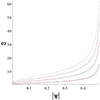Fig. 6. Alfvén continuum frequencies (ω) as a function of the flux line (|ψ|) in the case of a purely 2D X-point magnetic field (without a guide field) for the fundamental tone (solid line) and the first (dashed line), second (dash-dotted line), and third (dotted line) overtones. The frequencies are given in normalized form, i.e., in units of ωR.

3.3. General magnetic field in a pressureless plasma

We investigated the case in which a constant vertical guide field along the y-direction is included. Equations (36) and (37) are difficult to solve analytically. A particular case that can be of interest, for example, in the solar corona is the case of a pressureless (or cold) plasma, for which we took a vanishing thermal pressure: p = 0.

Under this assumption, Eqs. (36) and (37) reduces to

$$\begin{array}{c}\hfill {\omega }^2{\xi }_y+F\left({\displaystyle \frac{B_{0\chi }^2}{B_{0\chi }^2+B_{0y}^2}F(Q)}\right)=0,\end{array}$$(48)

$$\begin{array}{c}\hfill {\displaystyle {\omega }^2{\xi }_{\chi }-\frac{1}{B_{0\chi }}F\left(\frac{B_{0\chi }^2{B}_{0y}}{B_{0\chi }^2+B_{0y}^2}F(Q)\right)=0.}\end{array}$$(49)

We worked with a guide field B_0y ≠ 0, and therefore, the quantities ξ_y and ξ_χ are not the displacement components perpendicular and parallel to the total magnetic field in this case. Indeed, ξ_y and ξ_χ are the displacement components perpendicular and parallel, respectively, to the X-point magnetic field B_0p = B_0χ1_χ. New variables ξ_⊥ and ξ_∥, which represent the perpendicular and parallel displacement components with respect to B₀ = B_0p + B_0t, respectively, were thus introduced,

$$\begin{array}{c}\hfill {\xi }_{\perp }={\mathbf{1}}_{\perp }·\mathit{\xi }=\frac{1}{B_0}(B_{0\chi }{\xi }_y-B_{0y}{\xi }_{\chi }),\end{array}$$(50)

$$\begin{array}{c}\hfill {\xi }_{\Vert }={\mathbf{1}}_{\Vert }·\mathit{\xi }=\frac{1}{B_0}(B_{0y}{\xi }_y+B_{0\chi }{\xi }_{\chi }),\end{array}$$(51)

where the unit vectors 1_⊥ and 1_∥ in the directions perpendicular and parallel to B₀, respectively, are defined as

$$\begin{array}{c}\hfill {\displaystyle {\mathbf{1}}_{\perp }=\frac{{\mathit{B}}_0}{B_0}\times {\mathbf{1}}_{\psi },}\end{array}$$(52)

$$\begin{array}{c}\hfill {\displaystyle {\mathbf{1}}_{\Vert }=\frac{{\mathit{B}}_0}{B_0},}\end{array}$$(53)

with $B_0=||{\mathit{B}}_0||=\sqrt{B_{0\chi }^2+B_{0\mathit{y}}^2}$.

By rewriting Eqs. (48) and (49) in terms of ξ_⊥ and ξ_∥ and using Eq. (13) in its dimensionless form, the following governing equations were obtained for the displacement components inside a flux surface:

$$\begin{array}{cc}& {\displaystyle \{{\rho }_0{\omega }^2\frac{B_0^2}{B_{0\chi }{B}_{0y}}-\frac{1}{B_{0\chi }^5{B}_0^2}[2B_{0\chi }^4{B}_{0y}^3+2B_{0\chi }^6{B}_{0y}-4{\chi }^2{B}_{0y}^3}\hfill \\ \hfill & -16{\chi }^2{B}_{0\chi }^2{B}_{0y}+B_{0\chi }^4{B}_{0y}^5{k}_y^2+2B_{0\chi }^6{B}_{0y}^3{k}_y^2+B_{0\chi }^8{B}_{0y}{k}_y]\}{\xi }_{\perp }\hfill \\ \hfill & +\frac{4\chi B_0^2+2i{B}_{0\chi }^2{B}_{0y}{B}_0^2{k}_y}{B_{0\chi }{B}_{0y}}\frac{\partial {\xi }_{\perp }}{\partial \chi }+\frac{B_{0\chi }^3{B}_0^2}{B_{0y}}\frac{{\partial }^2{\xi }_{\perp }}{\partial \chi }=0,\hfill \end{array}$$(54)

$$\begin{array}{c}\hfill {\displaystyle \rho {\omega }^2\frac{B_0^2}{B_{0\chi }{B}_{0y}}{\xi }_{\Vert }=0.}\end{array}$$(55)

These equations are uncoupled from each other. Equation (55) shows that ξ_∥ = 0, and hence, that the slow wave has disappeared from the system, as is the case in a cold plasma. Equation (54) is a second-order ordinary differential equation for ξ_⊥ as a function of χ and governs the Alfvén continuum modes. The solution ${\stackrel{\sim }{\xi }}_{\perp }(\chi )$ of this equation is the regular part of the full solution ξ_⊥(ψ, χ, y). The equation has a complex coefficient, and hence, its solution is complex as well. The physically relevant part is then $\text{Re}[{\stackrel{\sim }{\xi }}_{\perp }(\chi )exp\{i(k_{\mathit{y}}\mathit{y}-\omega t)\}]$. We again drop the tilde from now on for clarity of notation.

We first investigated the special case where k_y = 0. Equation (54) then simplifies into

$$\begin{array}{cc}& {\displaystyle \{{\rho }_0{\omega }^2\frac{B_0^2}{B_{0\chi }{B}_{0y}}-\frac{1}{B_{0\chi }^5{B}_0^2}[2B_{0\chi }^4{B}_{0y}^3+2B_{0\chi }^6{B}_{0y}-4{\chi }^2{B}_{0y}^3}\hfill \\ \hfill & -16{\chi }^2{B}_{0\chi }^2{B}_{0y}]\}{\xi }_{\perp }+\frac{4\chi B_0^2}{B_{0\chi }{B}_{0y}}\frac{\partial {\xi }_{\perp }}{\chi }+\frac{B_{0\chi }^3{B}_0^2}{B_{0y}}\frac{{\partial }^2{\xi }_{\perp }}{\chi }=0,\hfill \end{array}$$(56)

whereas (55) remains unchanged. We note that Eq. (56) has real coefficients.

Equation (56) can be solved numerically on each flux surface. This is done by a shooting method, where we start at one side of the boundary and impose ξ_⊥ = 0 and $\frac{d{\xi }_{\perp }}{d\chi }=1$ there (the latter is arbitrary as it determines the amplitude). We then find the value of ω for which ξ_⊥ = 0 at the opposite boundary while having the required number of internal nodes as a function of the tone we wish to consider. The method for finding a solution on a particular flux surface ψ = ψ₀ has three steps:

1. take ξ_⊥(ψ₀, χ) = 0 and $\frac{d{\xi }_{\perp }(d{\psi }_0,\chi )}{\chi }=1$ as boundary conditions at $\chi =-\frac{\sqrt{-4{\psi }_0^2+1}}{2}$ and choose a value for ω as an initial guess,

2. solve the boundary value problem numerically,

3. modify ω and solve the boundary value problem again until ξ_⊥(ψ₀, χ) = 0 at the opposite boundary $\chi =\frac{\sqrt{-4{\psi }_0^2+1}}{2}$ with the required number of internal nodes.

The solutions ξ_⊥ as a function of s for the fundamental tone and first overtone in the flux surfaces from Fig. 3 with B_0y = 0, B_0y = 2, B_0y = 10, and B_0y = 100 are shown in Figs. 4 and 5. The profile varies slightly as the value of B_0y is changed, but overall, the profiles are very similar and the difference between the profiles for B_0y = 10 and B_0y = 100 cannot even be perceived. We stress that s is the arc length along the X-point magnetic field lines, which are different from the total magnetic field lines when B_0y ≠ 0. The plots thus show the displacement perpendicular to the total magnetic field line as a function of the arc length along the projection of that field line on the X-point plane. Figs. 4 and 5 show that the effect of the guide field decreases with increasing ψ value. For example, for the fundamental tone, when the value of the guide field increases from 0 to 2, for the case of ψ = 0.05, the maximum value of the displacement change is about 16%, while for the case of ψ = 0.25, the change value is about 2%. Moreover, the effect of the guide field in the fundamental tone is much higher than in the higher tones. When the guide field changes from 0 to 2, the maximum displacement value for the first overtone for the case ψ = 0.05 is about 2.5%, while this value is about 16% for the fundamental tone. Figs. 4 and 5 show that the maximum value of the displacement is insignificant when the value of the guide field is changed from 10 to 100. Therefore, it can be said that from a certain value for the guide field, the maximum value of the displacement does not change significantly. Figure 7 shows the Alfvén continuum frequencies of the fundamental mode as a function of the flux surface |ψ| for different values of B_0y. The values of the frequency are different for varying B_0y, but this difference becomes very small for higher values of B_0y.

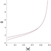Fig. 7. Alfvén continuum frequencies (ω) as a function of the flux surface (|ψ|) for the fundamental tone, with B0y = 0 (solid line), B0y = 2 (dashed line), and B0y = 10 (dotted line). The frequencies are given in normalized form, i.e., in units of ωR.

We investigated the more general case of k_y ≠ 0. In this case, the full complex differential equation (54) must be solved. This has a complex solution in general, the real part of which is the physically relevant solution. This was also discussed by Arregui et al. (2003) for Alfvén continuum modes, but in a different model. Figure 8 shows the profile of ξ_⊥ as a function of s in the flux surface |ψ| = 0.05 with B_0y = 2 and the ω of the fundamental tone for various values of k_y. Clearly, increasing k_y has the effect of creating a modulation in the profile. When k_y is nonzero, ξ_⊥ display a shorter-scale modulation along the flux surface. The results show that regardless of the value of k_y, the behavior of the vertical component of displacement is sinusoidal. This agrees with previous results. This was discussed by Halberstadt & Goedbloed (1993), who described a ballooning factor that caused this modulation in their analytical solution. The ballooning factor was also found by Arregui et al. (2003) in their analytical solution when k_y ≠ 0, and their solution was similarly modulated.

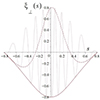Fig. 8. Perpendicular displacement (ξ⊥) of the fundamental tone of the Alfvén continuum mode as a function of the X-point magnetic field arc length (s) on the flux surface |ψ| = 0.05 with a nonvanishing guide field component B0y = 2 for ky = 0 (solid line), ky = 1 (dashed line), and ky = 10 (dotted line). The frequency of the fundamental tone of the case ky = 0 is used in each case.

4. Conclusion and discussion

We investigated the Alfvén continuum modes around an X-point magnetic field configuration. To this end, we defined a system of locally orthognal flux coordinates based on the directions along the field lines, normal to them and perpendicular to the X-point plane. We then used the set of equations derived by Goossens et al. (1985) that describe the continuum modes of the system to derive a set of two equations for the Lagrangian plasma displacement components perpendicular and parallel to the field lines within a given flux surface. Focusing our attention to Alfvén continuum modes, we found an analytical solution to the differential equation governing the regular part of the perpendicular displacement component (i.e., as a function of the coordinate along the magnetic field lines) in the case of a purely 2D X-point magnetic field. Assuming a cylinder with a circular cross section as a boundary to the system, we found an expression for the Alfvén continuum frequencies of the various tones under the boundary conditions of a vanishing displacement.

Next we investigated the case of an X-point with a guide field in a cold plasma by introducing a magnetic field component in the direction normal to the X-point plane. The equation for the perpendicular displacement was found to be too complicated to solve analytically, and we instead needed to solve it numerically through a shooting method by imposing the same boundary conditions of a vanishing displacement. We first considered the simplified case of a vanishing wavenumber in the direction of the guide field and found the Alfvén continuum frequencies for different values of the guide field strength. We found that the value of the frequency is influenced by the strength of the guide field, especially in the flux surfaces closer to the separatrixes forming the X-point shape. As the guide field increases, its effect decreases. Figure 7 shows that the difference between the frequency with B_y0 = 2 and B_y0 = 10 is insignificant, because the frequency seems to reach an asymptotic where it no longer depends on B_y0. We concluded by considering the case in which the wavenumber in the direction of the guide field does not vanish. In this case, the differential equation is complex and has a complex solution, the real part of which represents the physical displacement. The profile of the eigenfunction was shown to be modulated by the wavenumber component along the guide field, in accordance with earlier works that treated this matter.

The usefulness of deriving the Alfvén continuum modes lies in the fact that they form a complete orthogonal set, such that any perturbation can be written as a linear combination of these modes. The idea is to find the conditions of resonant absorption around an X-point and to assess the importance of the guide field and the component of the wavenumber aligned with it in this process. Resonant absorption might be investigated by applying the method used by Thompson & Wright (1993), who investigated regular and singular solutions around Alfvén resonances in two-dimensional systems. A similar analysis could be made here in flux coordinates, with an expansion of the displacement components in the form of Frobenius series solutions around a given flux line ψ = ψ₀. This would allow us to determine the necessary conditions for Alfvén resonance to occur and to find an expression for the jump that the different quantities make at the resonant position. Prokopyszyn et al. (2019) showed that the first three harmonic periods decrease as the flux function increases, which is consistent with our results in Fig. 6. Additionally, for different harmonics, when the flux function tends to zero, the value of the periodicity does not differ much, which is also consistent with our results. Resonance occurs at a point where the frequency equals the frequency of the Alfvén wave. Considering that in this paper, the frequency of the Alfvén wave is given by ${\omega }_R=B_R/(\sqrt{{\mu }_R{\rho }_R}{L}_R)$ and its value is constant, we can say that the resonance location is different for different harmonics. This finding also confirms the results presented by Prokopyszyn et al. (2019). Resonant absorption can have important effects on waves around X-points. This can be considered in future works.

Acknowledgments

This project received funding from the European Research Council (ERC) under the European Union’s Horizon 2020 research and innovation program (grant agreement No. 833251 PROMINENT ERC-ADG 2018).

References

Appendix A: General ordinary differential equations for ξ_χ and ξ_y

In this appendix we derive the differential equations (24) and (25). We recall the equations we start from, namely Eqs. (18)-(20) and (23), for the reader’s convenience:

$$\begin{array}{cc}& {\displaystyle {\rho }_0{\omega }^2{\xi }_{\chi }+\frac{1}{{\mu }_0{B}_{0\chi }}F({\mathit{B}}_0·{\mathit{B}}_1)-\frac{B_{0y}}{{\mu }_0{B}_{0\chi }}F\left(B_{1y}\right)=0,}\hfill \end{array}$$(A.1)

$$\begin{array}{cc}& {\displaystyle {\rho }_0{\omega }^2{\xi }_y+\frac{1}{{\mu }_0}F\left(B_{1y}\right)=0,}\hfill \end{array}$$(A.2)

$$\begin{array}{cc}& F\left({\displaystyle \frac{{\xi }_{\chi }}{B_{0\chi }}}\right)+\frac{1}{\gamma p_{0}J}\frac{\partial p_0}{\partial \chi }\frac{{\xi }_{\chi }}{B_{0\chi }}-\frac{B_{1\chi }}{B_{0\chi }}-\frac{B_{0\chi }{B}_{1\chi }+B_{0y}{B}_{1y}}{{\mu }_0\gamma p_0}=0,\hfill \end{array}$$(A.3)

$$\begin{array}{cc}& F\left(Q\right)-\left({\displaystyle B_{1y}-\frac{B_{0y}}{B_{0\chi }}{B}_{1\chi }}\right)=0,\hfill \end{array}$$(A.4)

where $F=\frac{1}{J}\frac{\partial }{\partial \chi }+i{k}_{\mathit{y}}{B}_{0\mathit{y}}$ is an operator and $Q={\xi }_{\mathit{y}}-\frac{B_{0\mathit{y}}}{B_{0\chi }}{\xi }_{\chi }$.

We start by rewriting Eq. (23) to isolate B_1χ. Using Eq. (14), this gives us:

$$\begin{array}{c}\hfill {\displaystyle B_{1\chi }=\frac{B_{0\chi }}{B_{0y}}{B}_{1y}-\frac{B_{0\chi }}{B_{0y}}F(Q).}\end{array}$$(A.5)

Similarly, we rewrite Eq. (20) to isolate B_1y:

$$\begin{array}{c}\hfill {\displaystyle B_{1y}=\frac{{\mu }_0\gamma p}{B_{0y}}F\left(\frac{{\xi }_{\chi }}{B_{0\chi }}\right)+\frac{{\mu }_0{B}_{0\chi }}{B_{0y}}\frac{\partial p}{\partial \chi }{\xi }_{\chi }-\frac{{\mu }_0\gamma p}{B_{0y}}\frac{B_{1\chi }}{B_{0\chi }}-\frac{B_{0\chi }{B}_{1\chi }}{B_{0y}}.}\end{array}$$(A.6)

Substituting the expression for B_1y from Eq. (A.6) into Eq. (A.5) and substituting the expression for B_1χ from Eq. (A.5) into Eq. (A.6) yields

$$\begin{array}{cc}\hfill B_{1\chi }=& {\displaystyle \frac{-B_{0\chi }{B}_{0y}}{B_{0y}^2+{\mu }_0\gamma p+B_{0\chi }^2}F(Q)+\frac{{\mu }_0\gamma p{B}_{0\chi }}{B_{0y}^2+{\mu }_0\gamma p+B_{0\chi }^2}F\left(\frac{{\xi }_{\chi }}{B_{0\chi }}\right)}\hfill \\ \hfill & +\frac{{\mu }_0{B}_{0\chi }^2}{B_{0y}^2+{\mu }_0\gamma p+B_{0\chi }^2}\frac{\partial p}{\partial \chi }{\xi }_{\chi },\hfill \end{array}$$(A.7)

$$\begin{array}{cc}\hfill B_{1y}=& {\displaystyle \frac{{\mu }_0\gamma p{B}_{0y}}{B_{0y}^2+{\mu }_0\gamma p+B_{0\chi }^2}F\left(\frac{{\xi }_{\chi }}{B_{0\chi }}\right)+\frac{{\mu }_0{B}_{0\chi }{B}_{0y}}{B_{0y}^2+{\mu }_0\gamma p+B_{0\chi }^2}\frac{\partial p}{\partial \chi }{\xi }_{\chi }}\hfill \\ \hfill & +\frac{{\mu }_0\gamma p+B_{0\chi }^2}{B_{0y}^2+{\mu }_0\gamma p+B_{0\chi }^2}F(Q).\hfill \end{array}$$(A.8)

These two latest equations give expressions for the unknowns B_1χ and B_1y in terms of the unknowns ξ_χ and ξ_y. We can now insert Eq. (A.7) and Eq. (A.8) into Eq. (19) and Eq. (18), to give us two coupled second-order differential equations for the Lagrangian displacement components ξ_χ and ξ_y:

$$\begin{array}{cc}& {\displaystyle \rho {\omega }^2{\xi }_y+\frac{1}{{\mu }_0}F[\frac{{\mu }_0\gamma p{B}_{0y}}{B_{0y}^2+{\mu }_0\gamma p+B_{0\chi }^2}F\left(\frac{{\xi }_{\chi }}{B_{0\chi }}\right)}\hfill \\ \hfill & +\frac{{\mu }_0{B}_{0\chi }{B}_{0y}}{B_{0y}^2+{\mu }_0\gamma p+B_{0\chi }^2}\frac{\partial p}{\partial \chi }{\xi }_{\chi }+\frac{{\mu }_0\gamma p+B_{0\chi }^2}{B_{0y}^2+{\mu }_0\gamma p+B_{0\chi }^2}F(Q)]=0,\hfill \end{array}$$(A.9)

$$\begin{array}{cc}& {\displaystyle \rho {\omega }^2{\xi }_{\chi }+\frac{1}{{\mu }_0{B}_{0\chi }}F[\frac{{\mu }_0\gamma p{B}_{0\chi }^2}{B_{0y}^2+{\mu }_0\gamma p+B_{0\chi }^2}F\left(\frac{{\xi }_{\chi }}{B_{0\chi }}\right)}\hfill \\ \hfill & +\frac{{\mu }_0{B}_{0\chi }^3}{B_{0y}^2+{\mu }_0\gamma p+B_{0\chi }^2}\frac{\partial p}{\partial \chi }{\xi }_{\chi }-\frac{B_{0\chi }^2{B}_{0y}}{B_{0y}^2+{\mu }_0\gamma p+B_{0\chi }^2}F(Q)]=0.\hfill \end{array}$$(A.10)

All Figures

	Fig. 1. Lines of constant flux coordinates ψ and χ. The solid lines show regions of constant ψ(x, z). These are the field lines of B0p. The dashed lines show regions of constant χ(x, z).
In the text

	Fig. 2. Studied system composed of an X-point configuration inside a circle and with a constant guide field perpendicular to it.
In the text

	Fig. 3. Flux lines (red) corresponding to |ψ| = 0.05 (left) and |ψ| = 0.25 (right), within the boundary circle (blue).
In the text

	Fig. 4. Perpendicular displacement (ξ⊥) of the fundamental tone of the Alfvén continuum mode as a function of the X-point magnetic field arc length (s) on the flux lines |ψ| = 0.05 (left) and |ψ| = 0.25 (right) for B0y = 0 (solid line), B0y = 2 (dashed line), B0y = 10 (dash-dotted line), and B0y = 100 (dotted line).
In the text

	Fig. 5. Perpendicular displacement (ξ⊥) of the first overtone of the Alfvén continuum mode as a function of the X-point magnetic field arc length (s) on the flux lines |ψ| = 0.05 (left) and |ψ| = 0.25 (right), for B0y = 0 (solid line), B0y = 2 (dashed line), B0y = 10 (dash-dotted line), and B0y = 100 (dotted line).
In the text

	Fig. 6. Alfvén continuum frequencies (ω) as a function of the flux line (|ψ|) in the case of a purely 2D X-point magnetic field (without a guide field) for the fundamental tone (solid line) and the first (dashed line), second (dash-dotted line), and third (dotted line) overtones. The frequencies are given in normalized form, i.e., in units of ωR.
In the text

	Fig. 7. Alfvén continuum frequencies (ω) as a function of the flux surface (|ψ|) for the fundamental tone, with B0y = 0 (solid line), B0y = 2 (dashed line), and B0y = 10 (dotted line). The frequencies are given in normalized form, i.e., in units of ωR.
In the text

	Fig. 8. Perpendicular displacement (ξ⊥) of the fundamental tone of the Alfvén continuum mode as a function of the X-point magnetic field arc length (s) on the flux surface |ψ| = 0.05 with a nonvanishing guide field component B0y = 2 for ky = 0 (solid line), ky = 1 (dashed line), and ky = 10 (dotted line). The frequency of the fundamental tone of the case ky = 0 is used in each case.
In the text

References

- Arregui, I., Oliver, R., & Ballester, J. L. 2003, A&A, 402, 1129 [NASA ADS] [CrossRef] [EDP Sciences] [Google Scholar]
- Craig, I. J. D., & McClymont, A. N. 1991, ApJ, 371, L41 [NASA ADS] [CrossRef] [Google Scholar]
- Craig, I. J., & Watson, P. G. 1992, ApJ, 393, 385 [NASA ADS] [CrossRef] [Google Scholar]
- Goossens, M., Poedts, S., & Hermans, D. 1985, Sol. Phys., 102, 51 [NASA ADS] [CrossRef] [Google Scholar]
- Goossens, M., Andries, J., & Aschwanden, M. J. 2002, A&A, 394, L39 [NASA ADS] [CrossRef] [EDP Sciences] [Google Scholar]
- Gruszecki, M., Vasheghani Farahani, S., Nakariakov, V. M., & Arber, T. D. 2011, A&A, 531, A63 [NASA ADS] [CrossRef] [EDP Sciences] [Google Scholar]
- Halberstadt, G., & Goedbloed, J. P. 1993, A&A, 280, 647 [NASA ADS] [Google Scholar]
- Hassam, A. B. 1992, ApJ, 399, 159 [NASA ADS] [CrossRef] [Google Scholar]
- Hassam, A. B., & Lambert, R. P. 1996, ApJ, 472, 832 [NASA ADS] [CrossRef] [Google Scholar]
- Heyvaerts, J., & Priest, E. R. 1983, A&A, 117, 220 [NASA ADS] [Google Scholar]
- Hollweg, J. V., & Yang, G. 1988, J. Geophys. Res., 93, 5423 [Google Scholar]
- Kadomtsev, B. B. 1966, Rev. Plasma Phys., 2, 153 [NASA ADS] [Google Scholar]
- Kaneko, T., Goossens, M., Soler, R., et al. 2015, ApJ, 812, 121 [NASA ADS] [CrossRef] [Google Scholar]
- Longcope, D. W., & Priest, E. R. 2007, Phys. Plasmas, 14, 122905 [NASA ADS] [CrossRef] [Google Scholar]
- McLaughlin, J. A., & Hood, A. W. 2004, A&A, 420, 1129 [NASA ADS] [CrossRef] [EDP Sciences] [Google Scholar]
- McLaughlin, J. A., De Moortel, I., Hood, A. W., & Brady, C. S. 2009, A&A, 493, 227 [NASA ADS] [CrossRef] [EDP Sciences] [Google Scholar]
- Ofman, L., Morrison, P. J., & Steinolfson, R. S. 1993, ApJ, 417, 748 [NASA ADS] [CrossRef] [Google Scholar]
- Prokopyszyn, A. P. K., Hood, A. W., & De Moortel, I. 2019, A&A, 624, A90 [NASA ADS] [CrossRef] [EDP Sciences] [Google Scholar]
- Sakurai, T., Goossens, M., & Hollweg, J. V. 1991, Sol. Phys., 133, 227 [Google Scholar]
- Santamaria, I. C., & Van Doorsselaere, T. 2018, A&A, 611, A10 [NASA ADS] [CrossRef] [EDP Sciences] [Google Scholar]
- Soler, R., Goossens, M., Terradas, J., & Oliver, R. 2013, ApJ, 777, 158 [Google Scholar]
- Thompson, M. J., & Wright, A. N. 1993, J. Geophys. Res., 98, 15541 [NASA ADS] [CrossRef] [Google Scholar]
- Van Doorsselaere, T., Kupriyanova, E. G., & Yuan, D. 2016, Sol. Phys., 291, 3143 [Google Scholar]