| Issue |
A&A
Volume 689, September 2024
|
|
|---|---|---|
| Article Number | A131 | |
| Number of page(s) | 19 | |
| Section | Planets and planetary systems | |
| DOI | https://doi.org/10.1051/0004-6361/202449433 | |
| Published online | 09 September 2024 | |
Sufficiency of near-surface water ice as a driver of dust activity on comets
Rethinking the old enigma
1
Max-Planck-Institut für Sonnensystemforschung,
Justus-von-Liebig-Weg 3,
37077
Göttingen,
Germany
2
Institute for Geophysics and Extraterrestrial Physics,
TU Braunschweig,
38106
Braunschweig,
Germany
3
Physikalisches Institut, University of Bern,
Sidlerstrasse 5,
Bern
3011,
Switzerland
4
Space Research Institute, Austrian Academy of Sciences,
Schmiedlstrasse 6,
8042
Graz,
Austria
5
Taras Shevchenko National University of Kyiv,
Glushkova ave. 2,
Kyiv,
Ukraine
6
Main Astronomical Observatory of National Academy of Science of Ukraine,
Akademika Zabolotnoho Str. 27,
03680
Kyiv,
Ukraine
7
Key Laboratory of Planetary Sciences, Purple Mountain Observatory, Chinese Academy of Sciences,
Nanjing
210008,
China
8
CAS Center for Excellence in Comparative Planetology, Chinese Academy of Sciences,
China
9
European Space Agency (ESA), ESAC,
Camino Bajo del Castillo s/n,
28692
Villanueva de la Cañada, Madrid,
Spain
Received:
31
January
2024
Accepted:
14
June
2024
Abstract
Context. Nearly all contemporary theoretical research on cometary dust activity relies on models depicting heat transfer and sublimation products within the near-surface porous layer. Gas flow exerts a pressure drag to the crust agglomerates, counteracting weak gravity and the tensile strength of that layer. Our interpretation of data from the Rosetta mission, and our broader comprehension of cometary activity, hinges significantly on the study of this process.
Aims. We investigate the role played by the structure of the near-surface porous layer and its associated resistance to gas flow, tensile strength, pressure distribution, and other characteristics in the scenario of the potential release of dust agglomerates and the resulting dust activity.
Methods. We employ a thermophysical model that factors in the microstructure of this layer and radiative heat conductivity. We consider gas flow in both the Knudsen and transition regimes. To accomplish this, we use methods such as test-particles Monte Carlo, direct-simulation Monte Carlo, and transmission probability. Our study encompasses a broad spectrum of dust-particle sizes.
Results. We evaluated the permeability of a dust layer composed of porous aggregates in the submillimetre and millimetre ranges. We carried out comparisons among various models that describe gas diffusion in a porous dust layer. For both the transition and Knudsen regimes, we obtained pressure profiles within a non-isothermal layer. We discuss how the gaps in our understanding of the structure and composition could impact tensile strength estimates. We demonstrate that for particles in the millimetre range, the lifting force of the sublimation products of water ice is adequate to remove the layer. This scenario remains feasible even for particles on the scale of hundreds of microns. This finding is crucial as the sublimation of water ice continues to be the most probable mechanism for dust removal.
Conclusions. This study partially overturns the previously held, pessimistic view regarding the possibility of dust removal via water sublimation. We demonstrate that a more precise consideration of various physical processes allows elevation of the matter of dust activity to a practical plane, necessitating a fresh quantitative analysis.
Key words: comets: general / comets: individual: 67P/Churyumov-Gerasimenko
Corresponding author; e-mail: This email address is being protected from spambots. You need JavaScript enabled to view it.
© The Authors 2024
 Open Access article, published by EDP Sciences, under the terms of the Creative Commons Attribution License (https://creativecommons.org/licenses/by/4.0), which permits unrestricted use, distribution, and reproduction in any medium, provided the original work is properly cited.
This article is published in open access under the Subscribe to Open model.
Open Access funding provided by Max Planck Society.
1 Introduction
The study of both periodic comets and exotic temporary objects of the Solar System, such as interstellar objects and long-period comets, is largely based on observations of dust activity, that is, the release of dust particles and the formation of the so-called dust coma. Our ability to model and predict the activity of these objects underlies the analysis and interpretation of observations. Numerous articles have been dedicated to the modelling the dust release, with attempts to address this issue dating back several decades. For instance, Rickman et al. (1990) proposed a model for the formation of a dust crust on the surface of a comet and examined the removal of particles due to the pulling force of sublimating ice. However, this model only considered the gravity of the nucleus as a counteracting force, and the authors assumed the cometary material to be non-cohesive and evaluated only the balance of forces acting on a detached dust grain. Despite its limitations, this approach remains widely used, as evidenced by its application in the work of Gundlach et al. (2015). The approach is very simple and allows us to estimate the maximum particle sizes that can be separated from the nucleus by gravity and gas-drag forces. The latter ability seems important as a zero approximation; for example, in order to obtain an estimation of total dust production. However, following the Rosetta mission, it is generally agreed that cohesive forces play a decisive role in our understanding of the behaviour of refractory cometary material. We direct the reader to the work of Blum et al. (2017), who present an analysis of observations made by various instruments on board the spacecraft.
One of the earliest studies to focus on the cohesion between dust grains and address the challenge of removing such particles within a physics-based model was conducted by Kuehrt & Keller (1994). This research considered dust particles of approximately 1 micron in size. Using a straightforward Hertzian model to describe interparticle cohesion, the authors observed that the anticipated strength of a porous, granular cometary dust mantle is several orders of magnitude greater than the gas pressure achievable in the surface layers. This led to the formulation of an unresolved issue often termed the ‘activity paradox’: despite observing strong cometary dust and gas activity, a functional model explaining dust release is yet to be established.
Skorov & Blum (2012) attempted to highlight a paradox that had been overlooked for many years. They demonstrated that the cohesion between dust particles could be significantly reduced if the hierarchical structure of these particles was considered. Following this, in Skorov et al. (2017) we used a thermophysical model that accurately describes heat transfer within a randomly porous layer and the cohesive force between dust aggregates. We conducted computer simulations on water and supervolatile ices situated beneath dust layers of varying thickness. Our examination revealed that the ratio of vapour pressure to the reasonably determined tensile strength for various agglomerate sizes and layer thicknesses provides compelling evidence that gas drag is insufficient to remove dust. We concluded that the sublimation of not only water ice but also supervolatile ice is incapable of removing small dust grains under illumination conditions corresponding to 1.3 au. It is important to note that our initial model incorporated several simplifications. While these simplifications allowed us to draw preliminary conclusions, they also introduced a degree of uncertainty. This uncertainty, in turn, served as a catalyst for the current research: here we aim to refine the model, reduce the simplifications, and thereby enhance the robustness of our conclusions. It is through this improved model that we strive to unravel the complex mechanisms governing the liberation of dust. Our previous research is centred on the activity of Comet 67P. Subsequently, Jewitt et al. (2019) arrived at a similar conclusion when considering the activity of new and long-period comets, thereby generalising the problem. In summary, the mechanism by which refractories are liberated to form the observed dust comae remains unclear.
To determine the next steps, we must consider the limitations (or simplifications) that were inherent in our previous model. It is important to note that this model was internally inconsistent to a certain degree. We used estimates for cohesion derived from porous aggregates, but concurrently, the microstructure of the layer and its transport characteristics were overly simplified. For permeability estimation, we referred to the results of Skorov et al. (2011), where the porous medium was depicted as a collection of straight cylindrical tubes. The layer was presumed to be homogeneous and composed of monomers. The thermal radiative conductivity, which can be dominant for submillimetre particles according to Gundlach & Blum (2012), was accounted for in a simplified manner. Solar radiation was considered to be absorbed solely on the surface, without penetrating into the high-porosity layer. Lastly, an unproven simple estimate was employed to calculate the gas-pressure drop within the layer.
All these shortcomings are eliminated in the modernised model presented below. This has become possible due to recent progress in the study of the transport characteristics of random porous layers and significant improvement of the heat model (Skorov et al. 2022; Skorov et al. 2023b; Skorov et al. 2023a). Below, these efforts are continued and expanded upon.
In the following sections, we outline the fundamental transport characteristics of the various porous layers under consideration, with a particular focus on hierarchical layers composed of large particles. We pay special attention to the case of inhomogeneous layers. For Knudsen diffusion, we employ the test-particle Monte Carlo (TPMC) method, as introduced in Skorov et al. (2011). We study an estimate of the gas-pressure drop for this mode based on the approach presented in Macher et al. (2024). Using the direct-simulation Monte Carlo (DSMC) method (Bird 1994), we also examine the transition regime of a gas flow, which may be relevant for grains of millimetre scale. Subsequently, we apply a new thermal model that more accurately accounts for radiative thermal conductivity (Skorov et al. 2023a). These results are based on the dense-medium radiative transfer (DMRT) theory (Tsang 1985) and the fast superposition T-matrix method (FaSTMM) (Markkanen & Yuffa 2017). To estimate the sublimation ability, we use the latest version of the modified quasi-stationary layered model of Skorov et al. (2023a). The excellent runtime of this model, which allows the analysis of many sets of model parameters, is offset by a simplified specification of the internal heat flow on a boundary condition at the sublimation front. We assess the applicability of this description using the transient 1D heat-transfer model, which includes an accurate estimation of heat flux into the nucleus (Skorov et al. 2016). Finally, we study the ratio between gas drag and layer cohesion to reanalyse the ‘cohesion bottleneck’ problem (Jewitt et al. 2019)1.
2 Gas diffusion through a porous layer
2.1 Zoo of dust porous layers
Prior to delving into a description of the transport characteristics necessary for calculating the gas drag force and pressure drop in a porous layer, we first provide a brief qualitative overview of the types of layers that are examined in this study. The categorisation of model layers can be structured based on diverse properties. We present one of the potential variants below. To characterise a particular layer, we employ two model parameters: the effective porosity and the characteristic size of the constituent particles.
The model layers were constructed either from solid spheres (monomers) or from porous aggregates (the so-called hierarchical layers). Layers of monomers were either mono-dispersed (spheres of the same size were used) or bi-dispersed (spheres of two sizes were used). In the latter case, the volume occupied by small spheres varied (from 15% to 60%), which led to a change in the average layer porosity. For mono-dispersed layers, various design methods were used: the method of Random Gravitational Deposition (RGD) and Random Sequential Packing (RSP). In the latter case, the minimum distance between pairs was positive, while in the former case, it was always zero. The spheres never overlapped. Hierarchical layers were built either with contact control (that is, aggregates always ‘touched’ each other) or without such control. In the latter case, the layer was built from pseudo-monomers, control spheres each of which contained a porous aggregate inside. So-called ballistic aggregates with double migration (BAM2) (Shen et al. 2008) were used as prototypes of these porous aggregates. Such aggregates have a porosity that decreases when approaching the centre of mass of the particle. Thus, by cutting out their central part, it is possible to reduce the effective porosity of the layer. However, even this trick does not allow the creation of a layer with a porosity lower than about 82–85%, which is a serious limitation of such a model when the monomer size is fixed.
The described layers have sufficient spatial homogeneity if we move away from the boundaries (faces) of the modelled region. To study the role of inhomogeneities, we artificially constructed layers containing either cavities (whose size is much larger than the size of sphere-monomer) or cracks (which are modelled using rectangular slits). In the first case, large spheres are removed from the initially bi-dispersed layers with a ratio of radii of 1:10, creating large voids. In the second case, half of the control volume is removed from a homogeneous dense layer with an initial porosity of about 65%, which increased the resulting porosity to about 85%. As a result of material removal, parallelepiped-shaped gaps are formed. An exhaustive description of the techniques used and limitations can be found in our recent papers: Reshetnyk et al. (2021), Skorov et al. (2021, 2022, 2023b), Reshetnik et al. (2022), An important limitation of all modelled layers is the achievable particle sizes. We must bear in mind that both ground and in situ observations provide strong evidence that the characteristic size of monomers is on the order of a micron or less. Consequently, our monomer layers are extremely finely dispersed. For aggregate layers, only densely packed porous particles containing several thousand monomers are used. These particles have a fractal dimension of 3, and their size is approximately equal to the cube root of the number of monomers multiplied by their size. Therefore, the size of our aggregates is on the order of 10 microns. This is almost an order of magnitude smaller than the desirable sizes where the dominant role of radiative heat conduction can be expected. However, when modelling Knudsen diffusion, dimensional quantities are not important, and only the ratios of, for instance, layer thickness to sphere size are significant. Based on this specific feature, we considered the diffusion of gas through a layer consisting of ‘virtual’ millimetre and even centimetre porous particles (Skorov et al. 2017). Strictly speaking, we made a deliberate assumption that the transport properties of layers of large porous particles do not noticeably differ from the properties of monomer layers. This was merely an intuitive guess at that time since we could neither construct a hierarchical layer nor calculate Knudsen diffusion in such layers.
The first known to us attempt to evaluate the transport characteristics of layers composed of very large (millimetre-scale) particles containing micron-scale monomers was made by Skorov et al. (2023b). It is important to note that a simple increase in the size of aggregates due to an increase in the number of monomers is not feasible if we aim to effectively simulate diffusion in a layer constructed from them. Clearly, a millimetre-size aggregate formed by a micron-sized monomer contains approximately billions of particles. Moreover, the size of the simulated space should be significantly larger than the size of the aggregates forming the layer. In a small volume, boundary effects become very prominent: for instance, the porosity near the side faces changes significantly (see, for example, the results of Güttler et al. 2023; and Laddha et al. 2023). Lastly, when using the TPMC method, it is necessary to use a large number of test particles to ensure the statistical sample size is sufficient (usually, we ensured that the layers are passed through by 10 000 test particles). All these factors necessitate the simulation of the diffusion of many thousands of test particles in a region containing many billions of scattering spheres, leading to unreasonably long simulation times for such model layers.
To circumvent this obstacle, Skorov et al. (2023a) proposed an indirect solution that enabled the consideration of transport in a hierarchical layer composed of millimetre-sized porous aggregates. The central idea of the proposed approach is that the vast majority of molecules colliding with a large aggregate, which is thousands of times larger than the size of the spherical monomers, scatter back, leaving the aggregate and scattering into the void between the aggregates. The defining characteristic of such a process is the distribution function of the offset of the exit points relative to the entry starting point. With this correction, the scattering event is modelled as scattering with an offset on a solid pseudo-monomer. In the cited work, we only considered the case where a large aggregate consists of spheres of the same size and has a porosity above 60%. Consequently, the effective porosity of the hierarchical layer of this configuration is high – it is close to the upper limit of physically reasonable values. In the following, we take the next anticipated step to reduce the effective porosity of the hierarchical layer.
For this purpose, we utilize the available bidisperse layers. It’s worth recalling that the porosity of these layers lies in the range of thirty percent, depending on the relative volume occupied by the larger particles (Skorov et al. 2021). These layers present two scenarios for creating hierarchical layers containing millimetre-sized aggregates. In the first scenario, we use the ‘parent’ layer of monomers and assume that only the larger monomers are porous aggregates containing solid spheres of the same size. The scattering on such pseudo-monomers is then calculated, taking into account the bias as was done in Skorov et al. (2023a). In the second scenario, we use a uniform monodisperse layer of monomers as the ‘parent’ layer. However, we consider all monomers to be porous aggregates of millimetre scale, containing hard monomers of two different sizes. Due to the bidispersity, the filling factor of such pseudo-monomers is approximately twice as high as in the previously used aggregates of the BAM2 type. As before, to work with these layers, we need to simulate the offset functions for back-scattered molecules. With this effect taken into account, Knudsen diffusion is modelled in the standard way.
Figure 1 illustrates the distribution of the displacement of the exit point relative to the entry point in the case of an aggregate composed of a bidisperse mixture of monomers, with an internal porosity of about 30%. In all considered cases, the model offset probability depicted in the lower panel is well approximated by a simple function. More technical details of the general approach and discussion can be found in (Skorov et al. 2023a). The improvement presented here is significant as it enables us to study hierarchical layers with porosity values closer to observational estimates. Lastly, we would like to emphasise that the type of scattering (diffuse or specular) has a noticeable impact on the specific form of the offset function. This was also the case when studying the permeability of layers (see discussion in Skorov et al. 2021; Skorov et al. 2022). Since we cannot estimate the scattering character for cometary dust, this uncertainty establishes the acceptable level of accuracy for the simulations.
2.2 Knudsen diffusion: basic transport characteristics
Based on the new modelling technique, we conducted, as before, a sequential evaluation of the transport characteristics of layers containing very large particles: starting with an analysis of the distribution of free paths or (which is the same for Knudsen diffusion) the distribution of chord lengths between collisions of test particles with the dust fraction, and ending with estimates of the mean free path (MFP) and layer permeability (Π), which are directly used in the heat transfer model. In this model, they have an impact on the effective thermal conductivity and sublimation rate, that is, the characteristics needed to estimate the pressure drop of the gas in the layer and its drag force. As in all previous cases, we constructed simple formulas that fit the results of numerical simulations. For both scenarios of constructing hierarchical layers containing large aggregates (~mm), the results differ very little from the results obtained for the corresponding “parent” layers with the obvious correction for the particle size. As a result of our simulations, we concluded that taking into account the offset of test particles (due to the propagation of the gas molecule inside the agglomerate, escaping it at a different position) does not have a significant impact on the transport characteristics of interest. This allows us to first use the approximating functions of the transport characteristics obtained earlier and second to use an analytical approach presented in detail in Macher et al. (2024) and used, for example, in Skorov et al. (2024).
Macher et al. (2024) presented a theoretical first-passage probability model assuming that the porous medium built by monodisperse spheres is homogeneous on a scale larger than the particle size and the molecule scattering is isotropic and diffuse. A bi-hemispherical Maxwell distribution model was applied, which was introduced by Asaeda et al. (1974), in this context. On this basis a formula was obtained having the same form as the empirical formulae for permeability used for the approximating numerical models in our recent publications (Reshetnyk et al. 2021; Skorov et al. 2021; Reshetnik et al. 2022; Skorov et al. 2022; Skorov et al. 2023b), namely
![Mathematical equation: $\[\Pi=\frac{1}{1+L / L_h},\]$](/articles/aa/full_html/2024/09/aa49433-24/aa49433-24-eq1.png) (1)
(1)
where L is the layer thickness and Lh the distance for which half the gas molecules incident on a model cuboid containing the scattering spherical monomers passes the layer through the pores. We note that this formula experimentally confirmed by Gundlach et al. (2011) is simpler and more general since it contains only one parameter, in contrast to the results of empirical fitting, which we obtained earlier and were different for different layers.
Based on Fick’s law for Knudsen diffusion and the model assumption about Maxwellian velocity distribution of the molecules the formula for Lh was given
![Mathematical equation: $\[L_h=\frac{4 D^K}{\phi v_{t h}(T)},\]$](/articles/aa/full_html/2024/09/aa49433-24/aa49433-24-eq2.png) (2)
(2)
where ϕ is porosity, ![Mathematical equation: $\[v_{t h}=\sqrt{\frac{8 k_B T}{\pi m_g}}\]$](/articles/aa/full_html/2024/09/aa49433-24/aa49433-24-eq3.png) is the mean thermal velocity, T is the temperature of the gas, kB is the Boltzmann constant, and mg is the mass of gas molecules.
is the mean thermal velocity, T is the temperature of the gas, kB is the Boltzmann constant, and mg is the mass of gas molecules.
Applying the results of (Derjaguin 1946) obtained under some simplifying assumptions about the chord length distribution (see details in Güttler et al. 2023; Macher et al. 2024) the relation between the MFP and the Knudsen gas diffusion coefficient DK can be obtained
![Mathematical equation: $\[D^K=\frac{3}{16} \phi \bar{\lambda} v_{t h}(T),\]$](/articles/aa/full_html/2024/09/aa49433-24/aa49433-24-eq4.png) (3)
(3)
where
![Mathematical equation: $\[\bar{\lambda} \equiv M F P=\frac{2 \phi}{3(1-\phi)} d_s,\]$](/articles/aa/full_html/2024/09/aa49433-24/aa49433-24-eq5.png) (4)
(4)
In Eq. (4), ds is the size of monomers and ![Mathematical equation: $\[\bar{\lambda}\]$](/articles/aa/full_html/2024/09/aa49433-24/aa49433-24-eq6.png) is the first moment of the chord length distribution.
is the first moment of the chord length distribution.
Substituting the results into the formula for Lh, we obtain the expression for the permeability
![Mathematical equation: $\[\Pi=\frac{1}{1+\frac{4}{3} L / M F P}.\]$](/articles/aa/full_html/2024/09/aa49433-24/aa49433-24-eq7.png) (5)
(5)
The obtained theoretical formulae are in good agreement with the approximations that were obtained in numerical models for homogeneous layers. A comparison of theoretical and numerical results for the MFP is shown in Fig. 2 for the hierarchical layers built from porous ballistic aggregates BAM2 of different sizes and for the layers of spherical monomers. The obtained relations make it easy to include the attenuation of the gas flow as well as the radiative conductivity depending on the MFP in the thermal model to calculate the resulting gas production.
In addition to the obtained theoretical estimates for MFP and permeability, the theoretical first-passage probability model allows one to obtain clear estimates for the gas density distribution within the isothermal diffuse scattering layer under stationary conditions. Following the presentation of Macher et al. (2024), under the assumption of an equilibrium velocity distribution of molecules due to their multiple diffuse scattering by dust particles, we can write an analogue of Fick’s first law for density flux. The vectorial flux can be written as a product of DK and the density gradient ∇n, so we find the equality
![Mathematical equation: $\[J=-D^{\mathrm{K}} \frac{\mathrm{d} n}{\mathrm{~d} z}=-D^{\mathrm{K}} \frac{\mathrm{d}}{\mathrm{d} z}\left(\frac{n^{+}+n^{-}}{2}\right).\]$](/articles/aa/full_html/2024/09/aa49433-24/aa49433-24-eq8.png) (6)
(6)
Here we define two hemispherical Maxwell distributions at each depth z, with number densities n+(z) and n−(z) inside the pores for particles with υz < 0 (moving downwards) and υz > 0 (moving upwards), respectively. The partial densities n+(z) and n−(z) are defined as double the actual densities of the particles moving in one direction, the total number density is the average n = (n+ + n−)/2. This assumption about the molecule velocity distribution was applied by Asaeda et al. (1974) to derive DK for a monodisperse packing of spheres. Because the mass flux J(z) is constant for a stationary flow, the last equation can be integrated over the layer height z to give a linear dependence of the density as a function of the distance from the entrance. Since we assumed a kinetic equilibrium for the gas in the layer, also the gas pressure P should be a linear function of height. This conclusion is fully supported by the results of the numerical simulation presented in Macher et al. (2024). It was shown (Fig. 5) that for a random porous layer of spheres of the same size (ϕ = 0.65), after just twenty milliseconds the density profile becomes linear over almost the entire thickness of the layer. This output is used below.
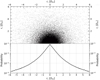 |
Fig. 1 Distribution of exit points for a given entry point at the origin of a bisdisperse agglomerate (top) and the probability distribution of the position of the exit point (bottom) as a function of the distance in size of the monomers. |
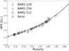 |
Fig. 2 Mean free path is shown as a function of layer porosity for uniform layers. Results are displayed for hierarchical layers (BAM2) and layers built out of monomers (Rand). Computational results (markers) and theoretical curves (solid lines) are shown. Different implementations of building a BAM2 aggregate and various numbers of monomers in an aggregate (from 128 to 512) were used for hierarchical layers. |
2.3 Transient flow of rarefied gas. Basic transport characteristics
In all previous models, the TPMC method was utilized. This method, in its classical version, is only applicable for simulating collisionless gas flow, that is, pure Knudsen diffusion in a random porous medium. The implementation of this method shares many similarities with random walk methods, as pointed out by Güttler et al. (2023) and Macher et al. (2024). The primary advantage of this method, its minimal runtime, is inherently linked with its main limitations. As we model the motion of a test particle, we essentially simulate only the direction of the ray (trajectory of movement) and do not consider either the time or the dynamic characteristics of the test particle (e.g. its speed). Therefore, this approach has significant limitations. It is challenging to simulate the effects caused by the energy exchange between the gas and the non-isothermal dust matrix. Without substantial modification, it is impossible to simulate unsteady gas flows. Finally, there are no direct methods to estimate the flows of mass and momentum inside the dust porous layer. All these issues are of undeniable interest to the physics of comets, which served as a motivation to expand the computer methods used henceforth.
The DSMC method developed by Bird (1976) is a highly attractive candidate. This method is extensively used to study rarefied gas flows, even in the absence of a kinetic equilibrium velocity distribution of molecules. In the field of cometary physics, this method has been widely employed for at least the past 40 years. While it is not our objective to provide an overview of its application here, it is worth noting that in most cases, different implementations of this method are used to study macroscopic external flows, such as the cometary atmosphere. There are only a few known examples of its application to study the internal flow of gas in a porous medium. We direct the reader to articles (Christou et al. 2018) and recent publications (Güttler et al. 2023 and Macher et al. 2024). The DSMC method enables also the simulation of collisionless gas flow. This case was analysed in Macher et al. (2024), where an excellent agreement between the results of the TPMC method and the DSMC method was demonstrated. In Güttler et al. (2023), intermolecular collisions were considered, but the authors did not provide the values of the Knudsen number, complicating the assessment of the degree of rarefaction of gas flow. In Christou et al. (2018), the method and its use are the primary focus of the study, but the authors provide little information about the flow in the layer, concentrating instead on studying the characteristics of the gas near the surface boundary of the layer. We employ the DSMC method to address these research gaps in the following sections.
We consider a monodisperse packing of 1 mm diameter particles. The domain is a parallelepiped of size 7.5 mm × 7.5 mm × L where L = 30 mm is the thickness of the dust layer. Two different porosities are studied with, a large one ϕ = 0.65 and a smaller one ϕ = 0.45. A sketch of the simulation setup is shown in Figure 3. At the inlet, the gas temperature Ti is imposed as well as its pressure P0 = Psat(Ti), where Psat is the saturation vapour pressure. The inlet velocity, which follows a half-Maxwellian distribution, is then imposed by the specific treatment of the pressure boundary condition proposed by Wang & Li (2004). The maximum gas production rate corresponding to these inlet conditions is then provided by the Hertz-Knudsen formula, giving a free-sublimation rate ![Mathematical equation: $\[Z_0=P_0 / \sqrt{2 \pi m_g k_B T_i}\]$](/articles/aa/full_html/2024/09/aa49433-24/aa49433-24-eq9.png) . As a result of collisions, both intermolecular and with the porous structure, some gas particles return to the inlet surface where a perfect condensing condition is assumed. This results in a reduction in the mass flow Z compared with the imposed mass flow Z0. The values of Ti, P0 and Z0 used in the DSMC simulations for both porosities are given in Table 1. For polyatomic gases, the variable soft sphere (VSS) model (Koura & Matsumoto 1991) is generally the most appropriate for modelling intermolecular collisions (Shen 2006). However, due to a lack of data for the water molecule, the variable hard sphere (VHS) model (Bird 1981, 1994) is used here instead. In this model, the collision diameter dVHS is a power law function of the relative collision velocity cr (Bird 1981)
. As a result of collisions, both intermolecular and with the porous structure, some gas particles return to the inlet surface where a perfect condensing condition is assumed. This results in a reduction in the mass flow Z compared with the imposed mass flow Z0. The values of Ti, P0 and Z0 used in the DSMC simulations for both porosities are given in Table 1. For polyatomic gases, the variable soft sphere (VSS) model (Koura & Matsumoto 1991) is generally the most appropriate for modelling intermolecular collisions (Shen 2006). However, due to a lack of data for the water molecule, the variable hard sphere (VHS) model (Bird 1981, 1994) is used here instead. In this model, the collision diameter dVHS is a power law function of the relative collision velocity cr (Bird 1981)
![Mathematical equation: $\[d_{V H S}=d_{r e f}\left(\frac{1}{\Gamma\left(\frac{5}{2}-\omega\right)}\left(\frac{4 k_B T_{r e f}}{m_g c_r^2}\right)^{\omega-1 / 2}\right)^{1 / 2},\]$](/articles/aa/full_html/2024/09/aa49433-24/aa49433-24-eq10.png) (7)
(7)
where Γ is the gamma function, dref − 4.597 × 10⁻¹⁰ m the reference diameter, Tref = 300K reference temperature and ω = 1.1 the temperature exponent for water (Crifo 1989). We treat all collisions as inelastic because water is a highly polar molecule with rapid equilibration (Combi 1996). For gas–dust interactions, we consider a diffusive reflection (Bird 1994) associated with a linear solid temperature Td given by
![Mathematical equation: $\[T_d=\left(1-\frac{z}{L}\right) T_s+T_i,\]$](/articles/aa/full_html/2024/09/aa49433-24/aa49433-24-eq11.png) (8)
(8)
where Ts and Ti are obtained from the thermal model (see Sect. 3) and given in Table 1. The solid phase temperature for the two porosity cases studied here is shown in Figure 4. At the side walls, a specular reflection condition is imposed (Bird 1994) while a vacuum condition is imposed at the outlet, which consists of eliminating the particles that pass through.
The initial mesh consists of a Cartesian grid of size 30 × 30 × 120. This is then refined using the snappyHexMesh utility of OpenFoam2. The refinement is performed on two levels in a non-conformal way to fit the spheres corresponding to the dust particles. The final mesh then contains about 2 million cells. An example of the mesh corresponding to the case ϕ = 0.65 is shown in Figure 5. Finally, the number of real particles represented by each DSMC particle is chosen to be 107, so that there is a sufficient number (>10) of simulated particles per cell (Bird 1994). The total number of simulated particles is then between 100 and 200 million, depending on the geometry considered.
The open source solver dsmcFoamPlus (White et al. 2018) implemented in the OpenFoam framework is used. It has previously been used to simulate flow in porous media on the surface of a comet (Christou et al. 2018, 2020; Mokhtari & Thomas 2024). The simulations are run in parallel, with each calculation requiring around 10 000 core hours.
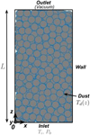 |
Fig. 3 Boundary conditions for three-dimensional DSMC simulations. Side view of a typical simulation domain. The domain consists of a parallelepiped of size 7.5 mm × 7.5 mm × L, where L is the dust-layer thickness. A gas temperature Ti and pressure P0 are imposed at the inlet surface (z = 0). For gas-solid interactions, a diffuse reflection of the gas particles is considered, where the dust temperature is Td(z). At the side walls, a specular reflection condition is considered. Finally, at the outlet surface (z = L), a vacuum condition is imposed. |
Boundary conditions imposed for DSMC simulations.
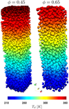 |
Fig. 4 Solid temperature Td distribution for a dust layer of thickness L = 30 mm and porosity ϕ = 0.45 (left) and ϕ = 0.65 (right). |
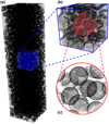 |
Fig. 5 Example of the mesh used for the DSMC simulations in the case where ϕ = 0.65. (a) Full mesh, (b) zoomed-in view, (c) zoom onto the solid surface mesh. The initial mesh is Cartesian and consists of about 100 000 cells. A two-stage local non-conformal refinement is then applied near the solid wall. The refined mesh contains about 2 million cells. The solid surface is described by around 750 000 faces. |
3 Thermophysical Model B
3.1 Heat equation
The surface of an evolved comet is typically enveloped by a porous, ice-free layer, which forms as the ice sublimates. The morphology of this layer, characterized by its thickness and porosity, remains akin to the pristine morphology of the underlying ice–dust mixture due to the cohesive forces and gentle sublimation process (Blum et al. 2017; Thomas et al. 2021).
To evaluate the feasibility of dislodging dust particles held together by cohesion, it becomes essential to estimate the temperature of the sublimating ice and the momentum flux of the gas acting on the non-volatile crust. The solution can be derived by solving the heat equation (Huebner et al. 2006). Considering the porous nature of the cometary material necessitates accounting for several physical effects, the significance of which escalates with the size of the dust particles. A contemporary overview of the situation can be found in Thomas (2021). In our previous work (Skorov et al. 2017), we initiated an analysis of the gas lifting force exerted on dust grains, taking into account the radiative heat conductivity of the layer and its cohesion. The results were promising for particles of millimetre size or larger. However, for smaller aggregates, the cohesive force significantly surpassed the lifting force, rendering the gas removal mechanism ineffective. It is noteworthy that the model used for the largest particles was overly simplified, with idealised approximations employed for both layer permeability and effective thermal conductivity. The substantial advancements in this field in recent years call for a revision of the model and the derivation of new estimates.
In the following, we solve a heat equation for a layered medium to determine the temperature of the sublimating ice boundary and the gas pressure. The general formulation of such a model can be traced back to the pioneering work of Fanale & Salvail (1984). Our primary simplification pertains to the assumption that the change in the outer boundary condition during the diffusion of molecules in the surface layer is negligible. Excluding unfavourable scenarios where, for instance, the surface experiences uneven irradiation (e.g. effects of shadow Macher et al. 2019 and roughness), this assumption appears reasonable for a slowly rotating nucleus. It should be noted that the model’s thermal conductivity is not assumed to be zero. Instead, our simplification corresponds to the assumption that the settling time of the temperature distribution in a thin near-surface layer is relatively short. This simplification is corroborated by observational estimates of thermal inertia (Schloerb et al. 2015), which is small, at least for unconsolidated surface material.
Our so-called Model B, discussed in detail in Keller et al. (2015b); Keller et al. (2015a) and further developed in Skorov et al. (2017), employs a 1D two-layer model of the nucleus. This model incorporates an effective heat conductivity that depends on temperature and layer resistance to gas flow. The cometary dust is treated as porous aggregates. Given that the characteristic time of gas and heat diffusion is short, surface erosion is not included in the model, rendering the layer thickness and porosity as fixed model parameters. The boundary conditions on the surface and at the lower boundary of the dust layer express energy conservation:
![Mathematical equation: $\[\left(1-A_v\right) I=\epsilon \sigma T_{{surface }}^4+\left.\frac{K_{eff}(T)}{1-\phi} \frac{d T}{d z}\right|_{z=0},\]$](/articles/aa/full_html/2024/09/aa49433-24/aa49433-24-eq12.png) (9)
(9)
![Mathematical equation: $\[\left.\frac{K_{e f f}(T)}{1-\phi} \frac{d T}{d z}\right|_{z=L^{+}}-\left.K_{e f f}^{\text {core }}(T) \frac{d T}{d z}\right|_{z=L^{-}}=\Pi Z\left(T_i\right) H,\]$](/articles/aa/full_html/2024/09/aa49433-24/aa49433-24-eq13.png) (10)
(10)
where I is the solar irradiation, Aυ is the bolometric Bond albedo3, ϵ is the emissivity, σ is the Stefan-Boltzmann constant, Z is the mass sublimation rate, H is the latent sublimation heat, and Π is the layer gas permeability that is a function of the layer thickness, porosity, and particle size. The mass sublimation rate is given by the Hertz-Knudsen formula, Z(T) = P(T)/(0.5πυth), where P(T) is the saturation vapour pressure, ![Mathematical equation: $\[v_{t h}(T)=\sqrt{8 R T / \pi \mu}\]$](/articles/aa/full_html/2024/09/aa49433-24/aa49433-24-eq14.png) is the thermal velocity of the vapour molecules, and μ is the molar mass. The variables Keff(T) and
is the thermal velocity of the vapour molecules, and μ is the molar mass. The variables Keff(T) and ![Mathematical equation: $\[K_{e f f}^{{core }}\]$](/articles/aa/full_html/2024/09/aa49433-24/aa49433-24-eq15.png) are the effective heat conductivities of the porous dust layer and the icy medium respectively. The inclusion of thermal conductivity within the region containing ice adds further complexity to the model. Therefore, to maintain a closed system of equations, it becomes essential to make simplifying assumptions regarding this factor. Some considerations is contemplated in this regard below. Moreover, it is crucial to acknowledge that the porosity within this region may vary significantly. For instance, assuming an equal volumetric content of ice and dust results in a doubling of the filling factor. It is important to highlight that the correlation between volatile and non-volatile substances remains a topic of ongoing debate. The predominant contribution to the effective thermal conductivity of the icy zone stems from contact thermal conductivity, which is believed to be small. Furthermore, supporting the insignificance of this factor on the processes in question is an analysis presented below. The model explicitly treats the solid and radiative part of the effective conductivity, which leads to a temperature dependence of the effective conductivity (Gundlach & Blum 2012). The presented formulas take into account that in the model of a porous layer, only part of the outer boundary is occupied by the solid phase where energy absorption and emission take place.
are the effective heat conductivities of the porous dust layer and the icy medium respectively. The inclusion of thermal conductivity within the region containing ice adds further complexity to the model. Therefore, to maintain a closed system of equations, it becomes essential to make simplifying assumptions regarding this factor. Some considerations is contemplated in this regard below. Moreover, it is crucial to acknowledge that the porosity within this region may vary significantly. For instance, assuming an equal volumetric content of ice and dust results in a doubling of the filling factor. It is important to highlight that the correlation between volatile and non-volatile substances remains a topic of ongoing debate. The predominant contribution to the effective thermal conductivity of the icy zone stems from contact thermal conductivity, which is believed to be small. Furthermore, supporting the insignificance of this factor on the processes in question is an analysis presented below. The model explicitly treats the solid and radiative part of the effective conductivity, which leads to a temperature dependence of the effective conductivity (Gundlach & Blum 2012). The presented formulas take into account that in the model of a porous layer, only part of the outer boundary is occupied by the solid phase where energy absorption and emission take place.
Accounting for this factor necessitates modifications to the heat transfer equation. The high porosity of the layer implies that even in an opaque medium, direct incident radiation can penetrate deeply into the surface. This process was initially modelled by Davidsson & Skorov (2002), subsequently confirmed in the laboratory (Kaufmann et al. 2006), and has since become a focal point of our research (e.g. Krause et al. 2011). The term describing volumetric energy absorption must be incorporated into the general thermal conductivity equation. We previously addressed this issue in the context of gas heating in the case of Knudsen free-molecular diffusion (Skorov et al. 2024). To estimate the lifting force within the layer, the DSMC method is preferable. The interplay of volumetric absorption and the collisional diffusion regime will be explored in our forthcoming work.
3.2 Effective heat conductivity
A systematic presentation of the approach to calculating the solid thermal conductivity in a porous medium from granular material is given in Gundlach & Blum (2012). The main advantage of this study is the description of the successive transition from bulk thermal conductivity to thermal conductivity between spherical monomers, and further to thermal conductivity of a layer of porous aggregates. One of the minor shortcomings of the outlined approach can perhaps be attributed only to an excessive intention to make the scheme too specific. So, the temperature dependence was added to the expression for the bulk thermal conductivity, which, if it takes place, differs for different compositions of the material. The composition of a material can significantly impact the temperature dependency of bulk thermal conductivity, as evidenced by laboratory tests conducted on meteorite samples. For contact heat conduction, an expression for spheres of the same size based on the Hertz theory is used. However, it should be borne in mind that polydispersity can change the value of this function. The same can be said about the consideration of packing spheres in a layer. The authors consider expressions obtained for regular configurations. Finally, the transition to hierarchical layers is made using the idea of “quasi-monomers” (similar to how it was done by Skorov et al. 2018). That is, the model is used without control over the contacts between the units. Despite all these shortcomings, the presented approach is very important and is widely used in cometary physics. When using it, one should only remember internal uncertainties, some of which were analysed by Skorov et al. (2023b). These uncertainties that cannot be eliminated today in some sense set the available accuracy with which one can determine the effective contact thermal conductivity of cometary material.
Similar criticism must be given for the analysis of radiative heat conduction. Numerous works have been devoted to the evaluation of this characteristic and its application to the physics of comets, we can refer the reader to the article by Skorov et al. (2023a). This article describes various popular descriptions of radiative heat conduction. All of them are united by the fact that thermal conductivity is proportional to the cube of the temperature with a certain factor (see discussion in van Antwerpen et al. 2010). Skorov et al. (2023a) compared idealised methods of determining this factor with a much more rigorous approach where the heat equation is solved and the DMRT (dense media radiative transfer) approach is used (Markkanen & Agarwal 2019, 2020). The results of in-depth computer simulation showed that for tested porous particles with sizes from 10 to 1000 microns and media with a filling factor less than 30%, the approximation proposed by Van der Held (1952) has the best agreement with the most rigorous sophisticated model (see Fig. 3 in the cited work). Van der Held’s formula in a vacuum coincides with that obtained by Merrill (1969) treating the radiation as a photon gas and based on the gas kinetic theory
![Mathematical equation: $\[K_{r a d}=\frac{16 \sigma T^3 l_{p h}}{3}, \quad l_{p h}=\frac{1}{\kappa_{s c a}+\kappa_{a b s}}.\]$](/articles/aa/full_html/2024/09/aa49433-24/aa49433-24-eq16.png) (11)
(11)
Here lph is the mean path length of photons, κsca + κabs is the mean extinction coefficient calculated over the entire wavelength range (κabs is the absorption coefficient, κsca is the scattering coefficient). Below we use the classical power-law dependence of radiative conductivity on temperature with a coefficient determined from computer simulations.
The radiative heat transfer mechanism within porous media is pivotal in numerous instances of planetary physics. This includes everything from the nuclei and dust coma of comets to the surfaces of the Moon and Mercury. It would be an oversimplification to confine ourselves to a single common formula. Each specific case necessitates consideration of the microstructure of the layers, as well as the size and chemical composition of their constituent particles. We direct the reader to papers where both theoretical and experimental study results are established (Arakawa & Ohno 2020; Arakawa et al. 2019; Arakawa et al. 2017; Bischoff et al. 2021; Bischoff et al. 2023; Sakatani et al. 2018; Sakatani et al. 2017) It is worth reiterating that any quantitative evaluations conducted using a thermal model must account for the incomplete knowledge of the model characteristics. This, in turn, necessitates further exploration of the sensitivity of the outputs to this situation (Skorov et al. 2023b).
In conclusion, when considering the mechanisms of thermal conductivity, we acknowledge the role of thermal conductivity due to gas diffusion. Incorporating this process into the existing model is challenging, as the thermal conductivity of the gas in the case of Knudsen diffusion is dependent on both the gas temperature and its density, which vary with depth. The investigation of this process necessitates further research and is thus omitted in this discussion. The study of this process requires additional research and is omitted hereafter. Preliminary estimates for millimetre-sized particles suggest that this mechanism does not significantly influence the sublimation of water ice.
The technique outlined above relies on the description of a porous medium made up of individual particles (solid or porous). Historically, a different approach has been used in cometary studies, where isolated pores in a continuum have been considered. This view goes back to Smoluchowski (1982) who used a formula derived by Maxwell (1873) in the frame of his effective media theory. In this model, spherical grains are embedded in a medium of different conductivity and they occupy a small fraction of the total volume. This approach was applied, for example by Espinasse et al. (1993), and Marboeuf et al. (2012) and its detailed review was presented in Prialnik et al. (2004). In agreement with the latter, we note that none of these approximations allows for a pore-size media description and remains semi-empirical. We don’t use this approach below.
3.3 Heat flux to interior
As we conclude this section, we address another crucial point – the boundary condition on the lower side (Eq. (10)). In an accurate formulation, this expression should account for the heat flow into the nucleus. The difference in heat fluxes ‘to’ and ‘from’ the boundary determines the sublimation rate. To close the system of equations, it is necessary to make a simplifying assumption regarding the heat flux into the nucleus. In Keller et al. (2015b), we used a linear approximation for this term:
![Mathematical equation: $\[\left.K_{e f f}^{{core }}(T) \frac{d T}{d z}\right|_{z=L^{-}}=K_{{eff }}^{\text {core }}\left(T_i\right)\left[T_i-T_{{core }}\right] / l_{{core }},\]$](/articles/aa/full_html/2024/09/aa49433-24/aa49433-24-eq17.png) (12)
(12)
where the equilibrium orbital temperature Tcore and orbital skin depth lcore were evaluated following McKay et al. (1986). The volume ratio of ice to dust assumed equals one. Estimating the effective thermal conductivity of an icy medium faces significant difficulties. To be precise, we must introduce into the model a whole series of new poorly known parameters, such as the mass ratio of the volatile and non-volatile fraction (this is the subject of much debate), a change in the contact area for ice particles (e.g. due to vapour recondensation), and finally, a change in porosity near the sublimation front. All this makes the model unreasonably complex and vague. Considering irreducible uncertainties in estimations of these parameters we use another way and assess the role of this term in the overall energy balance. If this is an insignificant additive, then one can use the simplest assumption that thermal conductivity does not change when moving to an icy environment (as it is implemented by Keller et al. 2015b; Hu et al. 2017).
The cost of such simplification must be evaluated by estimating the contribution of this term in a thermal model where a non-linear transient heat equation is solved (Skorov et al. 2016). We assume that on the surface there is an ice-free porous dust layer with a thickness much smaller than the size of the total simulated region. Layer thickness and other structural characteristics are considered not to change. Conditions describing the accurate energy balance are given at the layer boundaries. At the lower boundary of the modelled region, the heat flux is zero. The size of the modelled region is 30 m. The radius of the porous aggregate is 1 mm, the thickness of the dust layer is 5 mm, and the porosity is 70%. The presented model values seem reasonable and their specific values are not important in the considered analysis. Calculations performed for other model values showed no qualitatively different results. When calculating the thermal conductivity, both contact and radiative thermal conductivity are taken into account. For the solar irradiation we use realistic functions calculated for two facets on the nucleus surface from the terrain model, SPHAPE 7 (Preusker et al. 2017). These points are chosen to provide significantly different irradiation conditions: point 1 is in the Seth region and point 2 is in the Hatmehit region. The variations of the solar zenith angle at these two locations, as a function of time, are shown in Figure 6. Point 2 (Hatmehit region) represents polar summer conditions whereas point 1 (Seth region) refers to polar winter.
The simulation results are presented for distances of 3 au and 1.24 au in the left and right columns, respectively (Fig. 7). The upper row shows the temperature changes at the surface (red curves) and at the lower boundary of the dust layer (blue curves) during one rotation for the two selected points (dashed curves for Point 1 and solid curves for Point 2). For clarity, we also draw the changes of the corresponding solar zenith angles (thin dotted curves). The lower row shows energy flows: total absorbed energy (dotted curves), heat flux at the surface (red curves) and at the lower boundary of the dust layer (blue curves). Thus, the difference between the absorbed energy and the heat flux on the surface determines the fraction of energy spent on thermal radiation. The difference between the heat fluxes at the boundaries of the dust layer determines the energy spent for the sublimation of ice. From the results presented, one can recognise the relative importance of all the terms in the energy balance entering into the equations. At small heliocentric distances (near perihelion), even in the least favourable case (Point 1), the energy spent on sublimation is many times greater than the energy delivered deep into the core. This means that errors arising from approximating the corresponding heat flux cannot in any way change the qualitative character of the dependence of the gas production rate and a corresponding drag force. At larger heliocentric distances, the situation is different (lower left figure): Now the energy spent for sublimation can be comparable (Point 1) or even much less (Point 2) than the thermal energy pumped into the interior. However, gas production at this distance is about a few per cent of its maximum value. Since the issue of dust removal (or destruction of the crust) by a gas flow is considered, it is the region where sublimation is the main channel of energy dissipation that interests us. It means that the suggested simplification does not have significant influence on the considered problem.
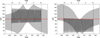 |
Fig. 6 Solar zenith angle as a function of time for points 1 (Seth) and 2 (Hatmehit). Y-axis: SZA in degrees. X-axis: Days from perihelion. Changes in the zenith angle in the vicinity of the perihelion are shown on a larger scale (upper X-axis). |
4 Lifting force and tensile strength
4.1 Saturation vapour pressure below the dust layer
The updated model presented above allows for a new analysis of the possibility of removing dust crusts under the influence of sublimation products. In this section, we present the results obtained for random porous layers shielding water ice. All of the modifications of this model should be most noticeable for water ice, which sublimates at a temperature of over 170 K. In the model version used, we 1) more consistently calculate radiative thermal conductivity, and 2) use new functions for permeability for all considered types of layers. Layers made of solid monomer spheres (1 μm), small porous aggregates (~10 μm) and large (~100 μm) porous dense aggregates are used as samples. Obviously, such layers have different characteristic void sizes and radiation attenuation depths. As a consequence, the roles of radiative thermal conductivity is also different even if the dimensionless thickness of layers is the same.
In our previous study (Skorov et al. 2017), we showed how the temperature and pressure at the sublimation front change for particles of different sizes and layers of different thicknesses. We emphasized that “different size” was a simple nonphysical scaling for the solid spheres used in that model. The calculations were presented only for two heliocentric distances and one porosity value. Now we can simulate realistic microphysical structures of different layers, consider a wide range of illumination values (which can be directly converted to heliocentric distance) and examine the role of porosity variation in dealing with the layer structure.
Figure 8 shows the ratio of temperatures (left column) and pressures (right column) at the boundary of the icy region. Particle types are indicated in the figure description. The layers are made up of monomers (top), small aggregates (middle), and large aggregates (bottom). For each pair of layers, we considered two porosity values: 70 and 80 per cent in the first case, 75 and 85 in the second, and 65 and 85 in the third. The relative increase in temperature is displayed in the left column as (Tl − Th)/Th, where Tl and Th represent temperatures for lower and higher porosity, respectively. The corresponding pressure ratio is presented in the right column. Radiation conductivity is enabled. There are only two mechanisms to increase the pressure under the layer. We can supply more energy available for sublimation, increasing the temperature of the ice and therefore the pressure. In addition, we can make the layer less transparent to gas by reducing permeability. Both of these mechanisms work in the updated model. Due to radiation thermal conductivity, we heat the ice more strongly. In addition, we also considered layers with lower permeability. All these effects are presented in Figures 8 and 9. The increase in pressure compared to the result obtained in the “bare exposed ice” model does not seem surprising. We note that if we move from porosity to a complementary value – the filling factor, then the changes in this characteristic are significant in the compared options. Considering the temperature ratio, we see that layers with higher filling have a small relative temperature increase at the icy interface. This excess decreases when moving from a layer of monomers to a layer of large particles. But even in the most promising case, it does not exceed 2–3%. This value may seem negligibly small, but here one should remember the exponential dependence of pressure on temperature. The results shown in the right column show that the pressure ratio is no longer insignificant and ranges from 2.2 (a maximum for a layer of monomers) to 1.7 (a maximum for a layer of large particles). Thus, we can conclude that local changes in porosity can cause a change in pressure under the layer several times. This conclusion is not obvious. Indeed, when we increase porosity we increase the average size of the voids. This growth causes an increase in radiative thermal conductivity, which is proportional to this characteristic. An increase in thermal conductivity contributes to a more efficient transfer of energy into the interior and an expected growth of temperature. At the same time, an increase in the size of voids leads to an increase in the permeability of the layer. This means that sublimation products are more easily evacuated (at the same relative layer thickness), and this already leads to a drop in temperature.
We note that the order of values for both temperatures and pressures does not change quantitatively when the particle size (and hence the characteristic dimensional thickness of the layer) increases by a hundred times. For the cases of small aggregates and monomers, even the shape of the surface remains similar, which is not the case for large particles. For large particles, a new effect is observed in the region where the illumination is low and the layer thickness is large. Low illumination “turns off” radiative thermal conductivity, the dimensional thickness of the layer is several millimetres and the energy flow at the ice boundary is no longer sufficient to increase the temperature in the layer with lower porosity. This effect is superior to that due to the lower permeability of the layer.
The input of radiation thermal conductivity is better visible for a layer of large particles according to the results shown in Figure 9. The top panel shows the ratio of effective thermal conductivity to contact thermal conductivity when hierarchical layers are considered. This relationship clearly shows that for the tested configurations the radiation mechanism dominates for all model cases. This is also because there are very few contacts between the micron-sized monomers that comprise our aggregates, ensuring a very low contact thermal conductivity in such a layer. The middle panel shows the increase in pressure under the layer compared to the model where the ice is on the surface (Model A). As one might expect, the higher the thermal conductivity, the more energy is supplied for sublimation. Since permeability decreases with increasing thickness and does not depend on illumination, the ratio reaches a maximum (about 7) for the thickest and most illuminated layer. Finally, in the bottom panel, we show the absolute pressure values at the ice boundary as a function of the thickness of the illumination. The maximum pressure values are already about 2 Pa, which is an order of magnitude greater than the “usual” expected vapour pressure of sublimating water ice.
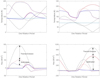 |
Fig. 7 Temperatures (top row) and energy fluxes (bottom row) as a function of time for points 1 and 2. The results are presented for distances of 3 au and 1.24 au in the left column and in the right column, respectively. The illumination functions are shown in Fig. 6. The upper row illustrates the temperature changes at the surface (red curves) and at the lower boundary of the dust layer (blue curves) during one rotation for the two selected points (dashed curves for Point 1 and solid curves for Point 2). The corresponding solar zenith angle is represented by thin dotted curves. The lower row plots the energy flows: total absorbed energy (dotted curves), and heat flux at both the surface (red curves) and the lower boundary of the dust layer (blue curves). |
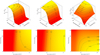 |
Fig. 8 Impact of layer porosity on both temperature and pressure beneath the layer as a function of absorbed energy and layer thickness. The relative increase in temperature is displayed in the left column. The corresponding pressure ratio is presented in the right column. The layers are made up of monomers (top), small aggregates (middle), and large aggregates (bottom). See main text for details. |
4.2 Lifting force
To estimate the lifting force exerted by the gas flow on the porous dust layer, several straightforward models can be employed. These models all rely on the saturated vapour pressure estimate discussed in the previous section. This parameter is frequently employed when analysing the preservation or erosion of the protective dust layer that lies atop the icy region. Many publications on cometary dust removal, e.g. Gundlach et al. (2015), Kuehrt & Keller (1994), typically use this approach. When translated into model geometry terms, this method corresponds to the simplest scenario where a solid, gas-proof cover is situated above the sublimation zone, providing us with a maximum estimate of the lifting force. The next significant improvement relates to porosity. In this scenario, only a portion of the infinitely thin lid experiences gas pressure, so the lift force directly correlates with the layer’s filling factor. This implies that for cometary porosities, there is a substantial reduction in lift. However, these evaluations are physically tenable, strictly speaking, only if we disregard the interactions between gas molecules and the dust skeleton – specifically, the backflow and associated inward momentum resulting from scattering. Moreover, these methods perceive the boundary between ice-free and ice-containing zones as a discontinuity where a qualitative change in the medium’s structure takes place. It is assumed that dust particles “float” over an area filled with ideal gas. This approach does not fully capture the complexity of the interactions and structural changes within the medium.
To properly evaluate the condition for dust removal, we need to compare the tensile strength with the pressure gradient within the porous layer. It is the pressure gradient, not the pressure itself, that creates the lifting force. A model that maintains the structural changes of the medium during the transition to an ice-containing zone and incorporates the interaction between the gas flow and the dust matrix can help overcome the limitations of a “standard” approach. In this scenario, estimating the lifting force requires computing the gas pressure profile (or gas molecule momentum) within the porous layer. This task is significantly more complex than the idealised approach previously discussed, even in the simplest case where the porous medium is homogeneous and isothermal, and the gas flow is stationary. The first attempt to estimate the pressure profile for this model, or more precisely the pressure drop in the layer, for Knudsen diffusion was made in Skorov et al. (2017). The accurate modelling of pressure within a random porous layer should be grounded in kinetic gas theory. However, in a first approximation, we can use results from estimations of the pressure gradient derived from knowledge of the layer’s permeability as a function of distance to the sublimating icy surface. Supposing the layer is isothermal and the gas is assumed to be in kinetic equilibrium (i.e. the distribution of molecule velocities obeys Maxwellian distribution), the pressure gradient can be estimated from differences in gas number density flows. In our prior research, two distinct permeability models for the layer were examined. The first is a modification of the Clausing function (Skorov et al. 2011), while the second is an experimental function derived for a gas flow through a monodisperse random porous layer (Gundlach et al. 2011). Unfortunately, both functions are quite approximate and should be used with appropriate caution. We could make only a qualitative note that for both permeability models, outside of the boundary zones, the gradient exhibited minimal variation, aligning with the linear behaviour of pressure as a function of distance from the sublimation front. Below we take the next step and apply kinetic approaches based on the analytical model (Macher et al. 2024) and on the use of the DSMC method applicable for the rarefied gas flow simulation to do a more reliable analysis of this crucial function.
We begin with the consideration of collisionless flow. Several related analytical approaches can be applied to find the pressure profile within the porous layer. Firstly, staying within the formalism used in studying the transmission probability of gas molecules for steady flow (Macher et al. 2024) one can conclude that the number density gradient is a constant in this case. Since it is assumed that the gas is ideal, the velocity distribution of molecules is Maxwellian and the layer is isothermal, this conclusion is also true for pressure related to the number density by the equation of state. In this case, pressure is a linear function of distance from the boundary of the icy region, that is
![Mathematical equation: $\[\mathbf{J}_{\mathbf{m}}=-\frac{D^K}{R T} \nabla P,\]$](/articles/aa/full_html/2024/09/aa49433-24/aa49433-24-eq18.png) (13)
(13)
where Jm free molecular flow flux, R is universal gas constant.
Since Jm is constant in steady states, the solution P(z) is a linear function P(z) = aPz + bP. The coefficients are determined from the pressure P0 = P(0) at the ice/dust interface and PL at the top of the layer.
The pressure PL is expressed in terms of Π and P0, using the densities n± of the upward- and downward-moving gas particles as introduced after Eq. (6), and their corresponding flux magnitudes
![Mathematical equation: $\[J^{ \pm}=\frac{n^{ \pm} \nu_{t h} \phi}{4}.\]$](/articles/aa/full_html/2024/09/aa49433-24/aa49433-24-eq19.png) (14)
(14)
Subscripts L and 0 are used for all location-dependent quantities to denote the respective values at z = L and z = 0. Since only a small fraction of the particles leaving the comet surface come back (caused by collisions of gas molecules outside the layer), we can assume ![Mathematical equation: $\[J_L^{+} \gg J_L^{-}\]$](/articles/aa/full_html/2024/09/aa49433-24/aa49433-24-eq20.png) . Therefore, the total flux is approximately equal to the escape flux
. Therefore, the total flux is approximately equal to the escape flux ![Mathematical equation: $\[J_L^{+}\]$](/articles/aa/full_html/2024/09/aa49433-24/aa49433-24-eq21.png) , and the gas flux
, and the gas flux ![Mathematical equation: $\[J_0^{-}\]$](/articles/aa/full_html/2024/09/aa49433-24/aa49433-24-eq22.png) returning to the ice/dust interface can be approximated as
returning to the ice/dust interface can be approximated as ![Mathematical equation: $\[J_0^{-}=(1-\Pi) J_0^{+}\]$](/articles/aa/full_html/2024/09/aa49433-24/aa49433-24-eq23.png) where
where ![Mathematical equation: $\[J_0^{+}\]$](/articles/aa/full_html/2024/09/aa49433-24/aa49433-24-eq24.png) is the sublimation rate (number of molecules per unit area and unit time). To arrive at the sought relation we express the product n νth at the layer boundaries,
is the sublimation rate (number of molecules per unit area and unit time). To arrive at the sought relation we express the product n νth at the layer boundaries,
![Mathematical equation: $\[n_L \nu_{t h, L}=\frac{2}{\phi}\left(J_L^{+}+J_L^{-}\right) \approx \frac{2}{\phi} J_L^{+}=\frac{2}{\phi} J_0^{+} \Pi,\]$](/articles/aa/full_html/2024/09/aa49433-24/aa49433-24-eq25.png) (15)
(15)
![Mathematical equation: $\[n_0 ~\nu_{t h, 0}=\frac{2}{\phi}\left(J_0^{+}+J_0^{-}\right) \approx \frac{2}{\phi} J_0^{+}(2-\Pi).\]$](/articles/aa/full_html/2024/09/aa49433-24/aa49433-24-eq26.png) (16)
(16)
Dividing the first by the second of these equations, and applying Eq. (4), yields the sought equation:
![Mathematical equation: $\[\frac{P_L / \sqrt{T_L}}{P_0 / \sqrt{T_0}}=\frac{n_L ~\nu_{t h, L}}{n_0 ~\nu_{t h, 0}}=\frac{\Pi}{2-\Pi}=\frac{1}{1+2 L / L_h}.\]$](/articles/aa/full_html/2024/09/aa49433-24/aa49433-24-eq27.png) (17)
(17)
This derivation assumes that the gas adopts the temperature of the solid matrix when collisions occur, and that the energy exchange between gas and dust does change the dust temperature to a negligible degree only. The result can be made plausible for isothermal layers with L ≫ Lh, for which PL = ΠP0/2: Since in this case Π ≪ 1, almost all gas molecules return to the ice, so ![Mathematical equation: $\[n_0^{-} \approx n_0^{+} \approx n_0\]$](/articles/aa/full_html/2024/09/aa49433-24/aa49433-24-eq28.png) and
and ![Mathematical equation: $\[n_L \approx n_L^{+} / 2=\Pi n_0^{+} / 2 \approx \Pi n_0 / 2\]$](/articles/aa/full_html/2024/09/aa49433-24/aa49433-24-eq29.png) .
.
Inside the layer the pressure drops linearly from P0 to PL, and the pressure profile can be obtained when the Knudsen diffusion coefficient DK and so the permeability Π are known. The linear dependence was confirmed on the basis of DSMC simulations by Macher et al. (2024). They have shown that the molecule number density of the gas flow dominated by Knudsen diffusion (no inter-molecular collisions) indeed approaches a stationary solution of linear height-dependence within milliseconds (see Figure 5 therein).
While the above treatment allows a temperature change across the layer under the mentioned preconditions, we have to assume isothermal conditions for the viscous flow case to facilitate an analytical treatment.
Now, we consider the other extreme case when the gas flow can be considered as a viscous flow. To derive the pressure profile in this case, we need to use the law of conservation of mass and the law of conservation of momentum in the form of Darcy’s filtration law. The model of single-phase filtration of compressible fluid in a non-deformable isotropic porous medium without taking into account gravity in general form is determined by the following system of equations:
![Mathematical equation: $\[\nabla \cdot(\rho \mathbf{v})=0,\]$](/articles/aa/full_html/2024/09/aa49433-24/aa49433-24-eq30.png) (18)
(18)
![Mathematical equation: $\[\mathbf{v}=-\frac{K_{\Pi}}{\mu} \nabla P,\]$](/articles/aa/full_html/2024/09/aa49433-24/aa49433-24-eq31.png) (19)
(19)
where ρ is the gas density, v is the velocity vector of the fluid, KΠ is the coefficient of permeability of the medium, μ is the dynamic viscosity of the fluid, and ∇P is the pressure gradient vector. Substituting Darcy’s equation into the mass conservation law and using the ideal gas state law in a one-dimensional case, we can rewrite this equation as:
![Mathematical equation: $\[-\frac{K_{\Pi}}{\mu}\left(\nabla P \cdot \nabla P+P \nabla^2 P\right)=0.\]$](/articles/aa/full_html/2024/09/aa49433-24/aa49433-24-eq32.png) (20)
(20)
At the steady state and spatially uniform layer, we can write
![Mathematical equation: $\[-\frac{K_{\Pi}}{\mu}\left[\left(\frac{d P}{d z}\right)^2+P \frac{d^2 P}{d z^2}\right]=0.\]$](/articles/aa/full_html/2024/09/aa49433-24/aa49433-24-eq33.png) (21)
(21)
This equation can be solved exactly. Thus, we obtain the well-known result
![Mathematical equation: $\[P(z)=P_0 \sqrt{1-\left(1-\frac{P_L^2}{P_0^2}\right) \frac{z}{L}}.\]$](/articles/aa/full_html/2024/09/aa49433-24/aa49433-24-eq34.png) (22)
(22)
This represents a pressure profile for a viscous flow in a porous medium under Darcy’s law with assumptions of conservation of mass and momentum.
In the transitional regime, the flow can be described as a superposition of the cases considered. The so-called Binary Friction Model (BFM) is a good approximation (Pant et al. 2012, Schweighart et al. 2021). For the molar particle flux, we can write:
![Mathematical equation: $\[\mathbf{J}=-\frac{K_{\Pi} P}{\mu R T} \nabla P-\frac{D^K}{R T} \nabla P,\]$](/articles/aa/full_html/2024/09/aa49433-24/aa49433-24-eq35.png) (23)
(23)
here the first term of the sum accounts for the viscous flow component and the second for the Knudsen flow component.
The solution of the generalised equation for the steady state one-dimensional case is
![Mathematical equation: $\[\begin{aligned}& \frac{P(z)}{P_0}=-\frac{D^K \mu}{K_{\Pi} P_0} \\& +\sqrt{1-\left(1-\frac{P_L^2}{P_0^2}\right) \frac{z}{L}+2 \frac{D^K \mu}{K_{\Pi} P_0}\left[1-\left(1-\frac{P_L}{P_0}\right) \frac{z}{L}\right]+\left(\frac{D^K \mu}{K_{\Pi} P_0}\right)^2}\end{aligned}.\]$](/articles/aa/full_html/2024/09/aa49433-24/aa49433-24-eq36.png) (24)
(24)
It is easy to see that the parameter b = μDK/KΠ (known as the Klinkenberg pressure) determines the contribution of various flow components and, as a result, the deviation of the pressure distribution in the layer from linear. The obtained formula for pressure differs from the one presented by Capelo et al. (2022). The formula presented there does not contain a term describing Knudsen diffusion at all. In addition, it can be shown that it is an approximation that is satisfactorily fulfilled only when P/b ≫ P0/P, i.e. when the pressure drops from P0 to P in the sample by a fraction (P0/P) much smaller than the remaining ‘fractional distance’ (P/b) from the Klinkenberg pressure. The given formulas allow for a quantitative assessment of the lift force acting on the porous layer, which is considered as a connected, non-deformable whole.
It is interesting to compare the above estimates obtained for limiting cases with the results of the numerical simulation of rarefied gas flow in the intermediate regime. Such modelling was carried out within the framework of the DSMC model described in detail earlier. A quantitative comparison of the results allows us to evaluate the applicability of the presented analytical approach.
Figure 10 shows the (normalised) pressure fields along a vertical cross-section for the two porosities considered. The relative pressure at the outlet PL/P0 is lower in the case of a denser dust layer, see Table 2, with which is reduced by a factor of about 3 between the cases ϕ = 0.65 and ϕ = 0.45. Consistently, the same is observed for relative production rate Z/Z0 (Table 2). It is important to note that the 3D pressure field is quite uniform on the monomer size scale: there are no noticeable “clumps” in the horizontal direction and the vertical distribution is quite uniform. The random orientation of elementary scattering facets and the diffuse reflection model provide effective “gas mixing”, that is, Maxwellization of the molecular velocity distribution. The state of a gas is indeed close to the simplest equation of an equilibrium ideal gas. This makes it meaningful to compare the results of DSMC modelling with the predictions of the presented analytical model.
In order to compare the results to the BFM, we define the average pressure profile
![Mathematical equation: $\[\bar{P}(z)=\frac{1}{\left|S_z\right|} \int_{S_z} P(x, y, z) d x d y,\]$](/articles/aa/full_html/2024/09/aa49433-24/aa49433-24-eq37.png) (25)
(25)
where Sz:= {(x, y, δ) in the fluid phase: δ = z} is the vertical fluid section at height z. A good agreement is observed between the results DSMC model and the BFM model, as shown in Figure 11. The value of the parameter b, obtained through fitting, is provided in Table 2. This value is close to 1, we are indeed in the transition regime, which is also confirmed by the ranges obtained for the Kn numbers (Table 2).
The presented results of numerical modelling show that the pressure profile inside the layer differs markedly from the idealised solution obtained for the collisionless regime when pressure is a linear function of depth. At the same time, the use of the BFM makes it possible to satisfactorily approximate the results obtained for the transition flow regime.
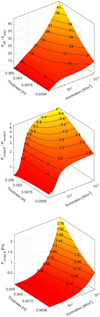 |
Fig. 9 Results for the layer built from large aggregates. Here, we show the ratio of conductivities (top panel), the ratio of the pressures in models B and A (middle panel), and the pressure below the dust crust (bottom panel) as a function of the absorbed energy and the layer thickness. |
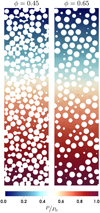 |
Fig. 10 Vertical cross-section across the dust layer for a thickness of L = 30 mm. Normalised gas pressure P/P0 in the case of porosity ϕ = 0.45 (left) and ϕ = 0.65 (right). |
Results obtained with the DSMC simulations.
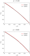 |
Fig. 11 Normalised gas pressure |
![Mathematical equation: $\[\bar{P} / P_0\]$](/articles/aa/full_html/2024/09/aa49433-24/aa49433-24-eq38.png)
4.3 Tensile strength
After examining the issue of gas pressure at the boundary of a dry dust layer and within it, we are ready to advance and explore the cohesion of a random porous layer formed by aggregates, that is, one possessing a hierarchical structure. In our previous research (2017), we employed a single formula to estimate the tensile strength of the layer, without considering the uncertainties and alternatives in studying this issue. Over the years, this problem has garnered significant attention, enabling us to present a more comprehensive analysis.
Skorov et al. (2017) made their investigation guided by the model proposed by Skorov & Blum (2012). In his model, the tensile strength of the dust aggregate layer σ is determined by its porosity and the size of the aggregates only and expressed in the following equation:
![Mathematical equation: $\[\sigma=\sigma_0(1-\phi)\left(\frac{R_a}{1 \mathrm{~mm}}\right)^{-2 / 3},\]$](/articles/aa/full_html/2024/09/aa49433-24/aa49433-24-eq39.png) (26)
(26)
where σ0 = 1.6 Pa is a constant, and Ra/1 mm denotes the dust aggregate radius, measured in millimetres. This formula is attractive due to its simplicity, although it contains some model idealisations hidden in the final equation. The proposed formula implicitly includes an estimate of the strength of a porous aggregate and explicitly includes a scaling law showing how it decreases with increasing aggregate size. To reveal the hidden parameters, we present a formula for the tensile strength of an aggregate following the impressive analysis presented by Kimura et al. (2020). The retrieved equation can be viewed as an extension of numerous formulas found in existing literature (refer to, for instance, Rumpf 1970, Kendall et al. 1987, Seizinger et al. 2013, Tatsuuma et al. 2019). When specific values are assigned to the free parameters within this equation, it simplifies to one of the known, less complex formulas. The tensile strength of a porous aggregate built by monomers of radius r0 is
![Mathematical equation: $\[\sigma=\left(\frac{4 \pi N}{3}\right)^{1 / m_W} \epsilon^{-1 / 2}\left(1-\phi_a\right)^{\beta-1 / m_W} n_{\mathrm{c}} \gamma r_0^{3 / m_W-1} V_a^{-1 / m_W},\]$](/articles/aa/full_html/2024/09/aa49433-24/aa49433-24-eq40.png) (27)
(27)
where N is the number of monomers in the aggregate, 1 − ϕa and ϵ denote the volume filling factor of the aggregate and a measure of the relative size of the flaws or defects within the aggregate compared to the size of the individual monomers, respectively, γ is the surface energy, Va is effective volume of the aggregate, β is a model parameter, and mW is commonly referred to as the Weibull modulus. A more detailed discussion of the parameters included in the equation can be found in the links in the cited work. The presented formula contains many parameters, each of which is known only approximately. The consideration of their variability is the subject of numerous articles. Thus, instead of a single simple estimate essentially expressing a scaling rule associated with aggregate size increase, we obtain a multidimensional space of model parameters. Their possible range of values provides an approximate estimate of the sought quantity.
Let us examine some of them that exhibit a significant degree of “cloudiness”. We introduce a substantial simplifying assumption, solely to facilitate comparison with the simulation results discussed in Kimura et al. (2020), assuming that the sizes of the monomer and aggregate are constant. (The role and estimates of these parameters are further elaborated in the subsequent discussion.)
We note that the size of the monomer and their number, together with porosity, are implicitly related to the volume of the aggregate so these parameters are not independent so that the given formula can be considered only as empirical or a fitting basis. All these parameters, including the aggregate’s porosity, are power-law dependent on the Weibull modulus, a parameter initially introduced for fractured media. Kimura et al. (2020) underscores that the values of this parameter are contingent on the particle composition and can exhibit significant variation (mw = 6–10 for amorphous silica, see references in the paper), thereby inducing causal alterations in the aforementioned parameters.
The next serious uncertainty is associated with the estimate of the surface energy γ. For the crystalline modification of silicates, a detailed discussion is given in the cited article (see Figure B1 there), based on an extensive array of published results. The summary indicates that estimates typically converge around γ = 1.5 J m−2 with a coefficient of variation of 2. Despite the considerable differences in surface energy values for amorphous silicates, there’s no compelling reason to assume that the scatter values would be significantly smaller. Brisset et al. (2016) derived the surface energy of a monomer particle by measuring the pull-off force of submm-sized dust aggregates from clusters. They utilised the scaling approach proposed by Weidling et al. (2012), yielding γ = 1.7 × 10⁻²J m−2 for monodisperse and 2.0 × 10⁻²J m−2 for polydisperse SiO2 particles. These values are consistent with the 2.5 × 10⁻²J m−2 measured for silica powder by Kendall et al. (1987) and 1.86 × 10⁻²J m−2 measured for approximately 1 μm SiO2 particles by Heim et al. (1999). Kimura et al. (2015) conducted a comprehensive analysis of the specific surface energy of amorphous silica. An exhaustive review of the existing literature was undertaken, revealing a significant discrepancy in the surface energy values reported by various researchers. This variation was attributed to the water content on the surface. The surface energy was estimated to be around 0.01 × 10⁻²J m−2 in the presence of water and approximately 0.2 × 10⁻²J m−2 in its absence. This indicates a substantial difference, with the surface energy in the dry case being an order of magnitude higher than in the wet case. Considering these observations, it is both reasonable and conservative to expect that the uncertainty of this parameter could be approximately a factor of 2–3. This underscores the importance of considering the presence or absence of water when measuring surface energy.
The value of the parameter β varies in different models from 1 (Skorov & Blum 2012; Rumpf 1970), to almost 2 (β = 2 Kendall et al. 1987, β = 1.88 Seizinger et al. 2013, β = 1.8 Tatsuuma et al. 2019). Another significant uncertainty in assessing the tensile strength is due to its direct dependence on the coordination number nc, which expresses the number of contacts between aggregates that should be destroyed when a pull-off force is applied4. A considerable amount of research has been dedicated to the investigation of the coordination number, often with the objective of correlating this parameter with porosity. While we do not delve into the specifics of the proposed models and methods, it is noteworthy that within the range of porosity values of interest to us, this characteristic can approximately double – ranging from 2 (which represents a solid low boundary) to 4–5.
It is important to acknowledge that so far we have not addressed significant aspects such as the polydispersity of particles (encompassing both monomers and aggregates), their nonsphericity, and, ultimately, microscopic surface roughness. Observational evidence of the Rosetta instruments (Bentley et al. 2016; Mannel et al. 2016; Moreno et al. 2016; Hilchenbach et al. 2016; Merouane et al. 2016) strongly suggests the presence of all these effects in cometary dust and pieces of the surface dust layer. These effects can influence the tensile strength, although quantifying their impact presents a considerable challenge. Under such conditions, estimates obtained in experiments become of great importance. Kimura et al. (2020) analysed the impact of listed effects. This work includes detailed comparisons of laboratory results with the proposed formula, demonstrating a quite satisfactory matching. Our interest, however, lies in a slightly different question: to what extent is the suggested estimate “floating” when many parameters are only approximately known? To answer this, we hypothesise that our model aggregates are BAM2-type particles (Shen et al. 2008), which we extensively utilise in studying transport and dynamic characteristics of cometary dust. For this scenario, we can employ known relationships that connect the aggregate volume and the number of monomers within it. We also obtain reliable estimates for the coordination number and filling factor of aggregate. All of this enables us to perform an inverse convolution of formula (27) to reduce the number of free model parameters and assess the uncertainty in estimating the final characteristic – the aggregate’s tensile strength. With the assumptions made, formula (27) takes the following form
![Mathematical equation: $\[\sigma=\tilde{A}\left(1-\phi_a\right)^\beta n_{\mathrm{c}} \gamma r_0^{-1} N^{-1 / m_W} \text {, }\]$](/articles/aa/full_html/2024/09/aa49433-24/aa49433-24-eq41.png) (28)
(28)
where à = Const. The term ![Mathematical equation: $\[\left(\frac{4 \pi N}{3}\right)^{1 / m_W} \epsilon^{-1 / 2}\]$](/articles/aa/full_html/2024/09/aa49433-24/aa49433-24-eq42.png) is treated as a constant in this simplification (see proof in Kimura et al. 2020). This made it possible to remove from the equation the characteristic ϵ associated with fracturing and arising due to the heterogeneity of the microstructure of the aggregate. Assuming that the size of the monomer, their number in the aggregate and the filling factor are given, we can show the variability of tensile strength σ as a function of the remaining three characteristics: surface energy γ, beta factor β, and the Weibull modulus mW. The obtained expression can be compared with the formula derived by Skorov & Blum (2012). Formula (28) assumes the same dependence on the input parameters β and size of aggregate as formula (26) if β = 1 and mW = 9/2.
is treated as a constant in this simplification (see proof in Kimura et al. 2020). This made it possible to remove from the equation the characteristic ϵ associated with fracturing and arising due to the heterogeneity of the microstructure of the aggregate. Assuming that the size of the monomer, their number in the aggregate and the filling factor are given, we can show the variability of tensile strength σ as a function of the remaining three characteristics: surface energy γ, beta factor β, and the Weibull modulus mW. The obtained expression can be compared with the formula derived by Skorov & Blum (2012). Formula (28) assumes the same dependence on the input parameters β and size of aggregate as formula (26) if β = 1 and mW = 9/2.
Based on the estimated intervals of parameter values included in expression (28), we consider how sensitive the tensile strength value is to the uncertainties that occur in the parameter values. The Figure 12 shows the relative changes in strength (assuming that the value of the effective constant including all fixed parameters is equal to one). The x, y, and z axes represent the β, γ, and mW/10, respectively. The size of the spheres depicted corresponds to the magnitude of the strength. The results show that the range of changes (from minimum to maximum) of the tensile strength is more than ten times. At the same time, the relative influence of each of the parameters being tested is comparable: it cannot be said that its changes can be neglected. Uncertainties arising from changes in monomer and aggregate sizes are no less important and are easily assessed. In the model under consideration, the strength is inversely proportional to the size of the monomer r0 and the number of particles in the aggregate N to the power of −1/mW. That is when the number of particles increases by three orders of magnitude and the aggregate size by approximately an order of magnitude, the force decreases approximately to 1000−2/9 ≈ 1/5 of its original value (since r0 remains the same) at typical values of mW.
Additional uncertainty which was not addressed above, is linked to polydispersity. This occurs both at the monomer level, significantly impacting the contact area between units, and at the aggregate level, influencing estimates of both pressure and tensile strength. The nonsphericity of the monomers and the micro-roughness of their surface may also contribute. Lastly, the presence of organic substances can substantially alter the assessment of free energy and, consequently, tensile strength.
The discussion above illustrates that theoretical estimates of tensile strength, in the absence of comprehensive information about the composition and microscopic structure of the medium, are largely speculative. Laboratory experiments, which are typically conducted with a known set of model parameters, can provide valuable insights. However, when generalising these results, it is crucial to remember the approximate types of scaling and dependencies previously discussed.
The strength of a porous medium composed of porous aggregates (i.e. a medium with a hierarchical structure encompassing different length scales) was examined by Blum et al. (2014) and Brisset et al. (2016). The former conducted a measurement of the tensile strength of loosely arranged dust aggregate samples (SiO2 clusters of porous aggregate with millimetre scale diameter). This experiment was carried out in two phases: initially, the samples were compressed using gas flow, and subsequently, the direction of the gas flow was reversed to ascertain the tensile strength of the granular samples. To obtain the uncompressed tensile strengths of the samples, the fit curves were projected to Δp = 0 Pa. The determined uncompressed tensile strengths of the dust-aggregate samples align well with the model proposed by Skorov & Blum (2012). In the latter study, an experiment on the REXUS 12 suborbital rocket was performed. The protoplanetary dust analogue materials were micrometre-sized monodisperse and polydisperse SiO2 particles prepared into aggregates with sizes around 120 μm and 330 μm. The tensile strength of aggregates in clusters was investigated in the SPACE experiment for aggregates composed of mono- and poly-disperse dust. The model is applied for aggregate filling factors of about 0.3–0.4. The data from the experiment are in good agreement with the model predictions that have no free parameters. The alignment of the findings from these independent experiments with the forecast of the model lends considerable credibility, particularly to the scaling methodology used by Brisset et al. (2016) and based on the model developed by Skorov & Blum (2012).
In the following section, we explore the possibility of dislodging a dust crust. This exploration is based on the estimates of tensile strength and their associated uncertainties presented earlier.
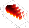 |
Fig. 12 Relative change in the tensile strength of the aggregate depending on the model parameters of equation (28). The x, y, and z axes represent the β, γ, and mW/10, respectively. The size of the spheres depicted corresponds to the magnitude of the strength. Porosity, number of monomers in the aggregate and their size are fixed. |
5 Discussion
Let us move on to analysing the possibility of dust crust removal by a gas flow. This task was considered in Skorov et al. (2017); however, as can be seen from the above, the development of the model and rethinking tensile strength estimates require an update of the analysis carried out earlier. First of all, this is due to new approaches that were used to estimate the permeability of the layer and its effective thermal conductivity. The latter leads to a change in both the heat equation and the boundary conditions. In turn, this changes the solution for the temperature profile in the layer.
At the first stage, we remain within the framework of the model proposed by Skorov & Blum (2012) for estimating the binding strength of the layer. This model does not contain free parameters. This is its strength and weakness at the same time. Its simplicity makes its use attractive and natural at the first step of the analysis. Figure 13 shows the results of calculations performed for a porous layer having a hierarchical structure and composed of aggregates having a radius of 1 mm (upper panel) and 0.1 mm (lower panel). As mentioned earlier, several characteristics can be analysed to determine the possibility of crust removal. In the simplest case, the layer tensile strength can be compared with the pressure under the crust estimated taking into account the porosity of the layer. This is the comparison shown in the figure under consideration. The modernisation of the model has led to qualitatively new results. For particles of millimetre size, a region has emerged for the first time where the effective gas pressure surpasses the tensile strength of the layer. For the parameter values determining tensile strength taken from Skorov & Blum (2012), its value for millimetre particles is about 0.64 Pa (depicted as a gray horizontal plane), and the portion of the pressure surface located above corresponds to the desired condition for the removal of the dust crust as a whole due to the lifting force of the gas flow.
Analysing the range of solar radiation values, three zones can be distinguished: in the first, the lifting force is less than the tensile strength at any considered values of thickness, in the second there is a zone where the lifting force is first less and then greater than the tensile strength, and in the third zone the ratio of these forces is always greater. Thus, depending on the energy received, three evolution scenarios are possible: in the first case, dust only accumulates and the layer remains stable, increasing in thickness; in the second, a repeating cycle of accumulation and shedding of the layer takes place, and in the third, a layer of large millimetre-sized particles alone cannot be formed because the radiation (and therefore the rate of sublimation) is too high.
The last note about the particle size is important. According to the scaling law for tensile strength (Eq. (26)), its value for aggregates of 0.2 mm in size escalates to approximately 3 Pa. The gas pressure for a layer of such aggregates also augments, but this increase is entirely insufficient. The maximum ratio of underlayer pressure to tensile strength in this embodiment is approximately 0.7 (lower panel). Consequently, we revert to the previous conclusion, which we now reformulate with the following statement: For illumination conditions on the surface of comet 67P for porous particles of 0.2 mm in size, the removal scenario does not arise, i.e. the effective pressure beneath the layer never surpasses the tensile strength of such a layer, calculated by the Eq. (26).
In the proposed formulation, the concluding part appears to be of significance. As noted, this formula for calculating tensile strength does not encompass free parameters. However, the discourse presented in the preceding section lucidly demonstrates that the tensile strength of aggregates (this characteristic is one level below the tensile strength of the layer if we consider the structure levels monomer-aggregate-layer) can undergo substantial alterations. By remaining within the plausible values of the free parameters incorporated in the formula for its estimation, one can procure values that diverge by more than an order of magnitude.
Let us contemplate how this uncertainty is translated to a higher echelon when we discuss the tensile strength of the layer. Pursuing the analysis presented by Weidling et al. (2012) and building on the approach utilising by Brisset et al. (2016), we can define a “scaled effective surface energy5”:
![Mathematical equation: $\[\xi_{{layer }} \sim N_c\left(1-\phi_a\right) \gamma_m^{5 / 3}\]$](/articles/aa/full_html/2024/09/aa49433-24/aa49433-24-eq43.png) (29)
(29)
where Nc is the number of connections from the separating aggregate to the cluster aggregates, γm is the surface energy of the constituent micrometre-sized monomer particles, ϕa is the aggregate porosity.
The deliberation presented in the previous section illustrates that the uncertainties inherent in the estimates of the parameters incorporated in this equation are so substantial that, while remaining within an acceptable range, we can effortlessly procure tensile strength below the pressure beneath the layer for the case of submillimetre particles too. This can be achieved through variations in surface energy estimates, alterations in the coordination number for the contacts between aggregates, and the dependence of tensile strength on the filling factor. All these uncertainties render it impossible to obtain reliable numerical estimates, and concurrently, the proximity of the obtained values for pressure and strength (see Fig. 13) does not permit us to exclude the destruction of the crust by the flow.
The above discussion is interesting on two levels. Firstly, as we see, even for particles with a characteristic size of about 100 microns, one can expect the removal of a layer due to the sublimation of water ice. Secondly, due to the strong increase in tensile strength as particle size decreases, it can be assumed that the zone in which a crust cannot form from millimetre-sized particles could drastically change when considering a mixture of particles of different sizes. These guesses require further theoretical but, first of all, experimental research.
So far we have compared tensile strength with the effective gas pressure under the layer P0. Strictly speaking, such an assessment is an idealisation, as we wrote earlier. A more precise approach involves computing the integral force exerted on the layer across its entire thickness, under the assumption that the layer behaves as a rigid solid body. We have demonstrated that the gas pressure profile varies with height either as a linear function or as the square root of the height, contingent on the gas flow regime. In both scenarios, calculating the integral over the full thickness of the layer presents no challenges. For a linear function, the pressure gradient is constant, and the estimate simplifies to the difference between the boundary pressure values. In the second scenario, when there is a transition gas flow regime the specific pressure drop diminishes with height non-linearly. This does not significantly alter the estimation of lift force, but changes the flow characteristics across the layer. It is also worth noting that numerical simulations conform that within the parameter value ranges of interest to us, the flow can be approximately described by the BFM, verifying that it is well is applicable for the low-end of the transition gas flow regime.
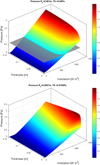 |
Fig. 13 Effective vapour pressure of sublimated water ice under a porous layer consisting of aggregates of radius 1 mm (top panel) and 0.1 mm (bottom panel) depending on the thickness of the layer and the incident solar energy. |
6 Conclusion
This study builds upon our previous work (Skorov et al. 2017), where we first attempted to quantify the potential for removing a porous dust layer with tensile strength through the flow of ice sublimation products. In that study, we explored the role of dust cohesion and the efficiency of near-surface ice sublimation in lifting dust particles (ranging from 1 μm to 1 mm) from the cometary nucleus surface. We presented results for a one-dimensional model of heat and mass transfer into a two-layer medium, where a near-surface sublimating ice–dust mixture is covered by an ice-free porous layer composed of monodisperse particles.
The primary and general limitation of the previous study was our inability at that time to accurately describe either the transport properties (such as layer permeability and average chord length inside the pores) or the thermophysical properties (such as radiative thermal conductivity) of layers composed of large porous aggregates. In other words, when discussing hierarchical layers, we were referring to layers composed of pseudo-monomers. Furthermore, to estimate the gas pressure distribution within the layer and the resulting lift force, we employed a simplistic approach without providing sufficient evidence of its accuracy. Lastly, when analysing tensile strength, we used a fixed formula, which presupposes reliable knowledge of the composition and microstructure of the porous layer.
The primary aim of this study is to address all the aforementioned weaknesses of our previous work and to provide a new analysis of a fundamental issue in cometary physics. We examined the removal of dust grains under the influence of a gas flow, drawing on the results of our studies published subsequent to Skorov et al. (2017).
In the first part of the present study, we concentrate on deriving precise expressions for layer permeability and mean chord length within pores (equivalent to the mean free path in terms of molecular gas dynamics). To enhance reliability, we employed and integrated various computational approaches. For the Knudsen diffusion mode, where there are no collisions between molecules, we applied the test-particles Monte Carlo (TPMC) method and an analytical model based on the transmission probability of gas molecules. For the regime of rarefied gas flow with molecule collisions, we applied the direct-simulation Monte Carlo (DSMC) method and the binary friction model, which describes the flow as a superposition of two limiting flow regimes.
To estimate the effective thermal conductivity, we referred to the results of our previous research, where we applied the approach of geometric optics and the theory of radiative transfer in a dense medium.
These advancements enable us to calculate both the ice temperature beneath the porous irradiated dust layer and the gas vapour pressure with greater reliability. Of particular importance is our meticulous modelling of the pressure distribution within the non-isothermal dust layer. In this context, we account for both the change in flux density due to the layer’s resistance and the change in the kinetic energy of molecules during collisions with the solid dust skeleton and among themselves. We devote significant attention to the critical analysis of the tensile strength of a layer, a characteristic that undoubtedly plays a crucial role in our study. At the same time, as we highlighted earlier (Skorov et al. 2023b), our understanding of many micro-properties of the materials under investigation is inherently limited and marked by a high degree of uncertainty. This highlights the importance of conducting a qualitative analysis of potential variations in tensile strength values. Our estimates indicate that this characteristic can vary by almost an order of magnitude, depending on the local composition and structure of the non-volatile substance. This analysis provides robust confirmation of the well-known empirical expectation: ‘a chain is only as strong as its weakest link’.
Building upon the improvements we have made, we evaluated the likelihood of a porous dust layer being destroyed by the flow of sublimating water ice products. We selected water ice specifically because it is the primary volatile component of most short-period comets within our focus. Our findings show that by selecting tensile strength values from the median of the possible range, we can convincingly demonstrate the potential for dust removal and the destruction of a millimetre particle layer. In this scenario, the ‘wave’ evolution we previously mentioned (Skorov & Blum 2012) comes into play: the phase of dust accumulation (increase in layer thickness) ends with the layer being ‘blasted off’. For certain irradiance values, the layer does not reset, and for excessively high irradiance values, a new layer cannot form after the reset. For a layer composed of particles of 100 microns, the ‘average’ tensile strength values are too high. However, by staying within the range of reasonable values, it is possible to envision a scenario where this layer is destroyed.
Our results provide a physically plausible explanation for dust activity resulting from the sublimation of water ice. It is worth noting that the microscopic model of the dust layer and the gas diffusion model presented in this work are currently the most advanced. In our forthcoming research, we will concentrate on identifying the ‘weak link’. Our investigation will encompass the examination of pressure distribution within hierarchical and heterogeneous layers, specifically those with slits and cavities. We previously conducted studies on the permeability of such layers in the context of collisionless flows. Our subsequent focus will be on transient flow regimes. For all processes under consideration, we will, for the first time, take into account the role of particle polydispersity, their non-sphericity, and surface microroughness. Regarding the aspect of heat transfer, our emphasis will be on incorporating the volumetric effects of radiation absorption and emission. A first step in this direction has already been taken (Skorov et al. 2024).
The principal conclusion drawn from this study serves to partially negate the wholly pessimistic conclusion regarding dust removal, as stated in our preceding research. We have demonstrated that a more precise consideration of diverse physical processes facilitates the transition of the issue of dust activity – which can be attributed to water ice sublimation – to a pragmatic level that necessitates a fresh quantitative analysis. This shift in perspective underscores the importance of accuracy in accounting for various physical phenomena in our ongoing research.
Acknowledgements
Yu.S. acknowledges support from ESA through contract 4000141229/23/ES/CM and the Deutsche Forschungsgemeinschaft (DFG) for support under grant BL 298/32-1. O.M. acknowledges the NCCR PlanetS supported by the Swiss National Science Foundation under grants 51NF40_182901 and 51NF40_205606. Y.Z. thanks the National Natural Science Foundation of China (Grant Nos. 12222307 12073084), and the CAS PIFI project (Grant No. 2022VMB0010).
References
- Arakawa, S., & Ohno, K. 2020, MNRAS, 497, 1166 [NASA ADS] [CrossRef] [Google Scholar]
- Arakawa, S., Tanaka, H., Kataoka, A., & Nakamoto, T. 2017, A&A, 608, A7 [NASA ADS] [CrossRef] [EDP Sciences] [Google Scholar]
- Arakawa, S., Tatsuuma, M., Sakatani, N., & Nakamoto, T. 2019, Icarus, 324, 8 [NASA ADS] [CrossRef] [Google Scholar]
- Asaeda, M., Yoneda, S., & Toei, R. 1974, J. Chem. Eng. Japan, 7, 93 [CrossRef] [Google Scholar]
- Bentley, M. S., Schmied, R., Mannel, T., et al. 2016, Nature, 537, 73 [Google Scholar]
- Bird, G. A. 1976, NASA STI/Recon Tech. Rep. A, 76, 40225 [NASA ADS] [Google Scholar]
- Bird, G. A. 1981, Prog. Astronaut. Aeronaut., 74, 239 [Google Scholar]
- Bird, G. A. 1994, Molecular Gas Dynamics and the Direct Simulation of Gas Flows (Oxford University Press) [CrossRef] [Google Scholar]
- Bischoff, D., Gundlach, B., & Blum, J. 2021, MNRAS, 508, 4705 [CrossRef] [Google Scholar]
- Bischoff, D., Schuckart, C., Attree, N., Gundlach, B., & Blum, J. 2023, MNRAS, 523, 5171 [NASA ADS] [CrossRef] [Google Scholar]
- Blum, J., Gundlach, B., Mühle, S., & Trigo-Rodriguez, J. M. 2014, Icarus, 235, 156 [Google Scholar]
- Blum, J., Gundlach, B., Krause, M., et al. 2017, MNRAS, 469, S755 [Google Scholar]
- Brisset, J., Heißelmann, D., Kothe, S., Weidling, R., & Blum, J. 2016, A&A, 593, A3 [NASA ADS] [CrossRef] [EDP Sciences] [Google Scholar]
- Capelo, H. L., Kühn, J., Pommerol, A., et al. 2022, Rev. Sci. Instrum., 93, 104502 [NASA ADS] [CrossRef] [Google Scholar]
- Christou, C., Dadzie, S. K., Thomas, N., et al. 2018, Planet. Space Sci., 161, 57 [NASA ADS] [CrossRef] [Google Scholar]
- Christou, C., Dadzie, S. K., Marschall, R., & Thomas, N. 2020, Planet. Space Sci., 180, 104752 [NASA ADS] [CrossRef] [Google Scholar]
- Combi, M. R. 1996, Icarus, 123, 207 [NASA ADS] [CrossRef] [Google Scholar]
- Crifo, J. 1989, A&A, 223, 365 [NASA ADS] [Google Scholar]
- Davidsson, B. J. R., & Skorov, Y. V. 2002, Icarus, 159, 239 [CrossRef] [Google Scholar]
- Derjaguin, B. 1946, AN SSSR, 53, 687 [Google Scholar]
- Espinasse, S., Coradini, A., Capria, M. T., et al. 1993, Planet. Space Sci., 41, 409 [NASA ADS] [CrossRef] [Google Scholar]
- Fanale, F. P., & Salvail, J. R. 1984, Icarus, 60, 476 [NASA ADS] [CrossRef] [Google Scholar]
- Gundlach, B., & Blum, J. 2012, Icarus, 219, 618 [CrossRef] [Google Scholar]
- Gundlach, B., Skorov, Y., & Blum, J. 2011, Icarus, 213, 710 [Google Scholar]
- Gundlach, B., Blum, J., Keller, H. U., & Skorov, Y. V. 2015, A&A, 583, A12 [NASA ADS] [CrossRef] [EDP Sciences] [Google Scholar]
- Güttler, C., Rose, M., Sierks, H., et al. 2023, MNRAS, 524, 6114 [CrossRef] [Google Scholar]
- Heim, L.-O., Blum, J., Preuss, M., & Butt, H.-J. 1999, Phys. Rev. Lett., 83, 3328 [NASA ADS] [CrossRef] [Google Scholar]
- Hilchenbach, M., Kissel, J., Langevin, Y., et al. 2016, ApJ, 816, L32 [CrossRef] [Google Scholar]
- Hu, X., Shi, X., Sierks, H., et al. 2017, MNRAS, 469, S295 [NASA ADS] [CrossRef] [Google Scholar]
- Huebner, W. F., Benkhoff, J., Capria, M.-T., et al., 2006, Heat and Gas Diffusion in Comet Nuclei (ESA Publications Division, The Netherlands) [Google Scholar]
- Jewitt, D., Agarwal, J., Hui, M.-T., et al. 2019, AJ, 157, 65 [NASA ADS] [CrossRef] [Google Scholar]
- Kaufmann, E., Kömle, N. I., & Kargl, G. 2006, Icarus, 185, 274 [NASA ADS] [CrossRef] [Google Scholar]
- Keller, H. U., Mottola, S., Davidsson, B., et al. 2015a, A&A, 583, A34 [NASA ADS] [CrossRef] [EDP Sciences] [Google Scholar]
- Keller, H. U., Mottola, S., Skorov, Y., & Jorda, L. 2015b, A&A, 579, A5 [NASA ADS] [CrossRef] [EDP Sciences] [Google Scholar]
- Kendall, K., McN. Alford, N., & Birchall, J. D. 1987, Proc. Roy. Soc. Lond. Ser. A, 412, 269 [NASA ADS] [CrossRef] [Google Scholar]
- Kimura, H., Wada, K., Senshu, H., & Kobayashi, H. 2015, ApJ, 812, 67 [NASA ADS] [CrossRef] [Google Scholar]
- Kimura, H., Wada, K., Yoshida, F., et al. 2020, MNRAS, 496, 1667 [NASA ADS] [CrossRef] [Google Scholar]
- Koura, K., & Matsumoto, H. 1991, Phys. Fluids A: Fluid Dyn., 3, 2459 [NASA ADS] [CrossRef] [Google Scholar]
- Krause, M., Blum, J., Skorov, Y., & Trieloff, M. 2011, Icarus, 214, 286 [NASA ADS] [CrossRef] [Google Scholar]
- Kuehrt, E., & Keller, H. U. 1994, Icarus, 109, 121 [NASA ADS] [CrossRef] [Google Scholar]
- Laddha, S., Macher, W., Kargl, G., et al. 2023, Meas. Sci. Technol., 34, 045012 [NASA ADS] [CrossRef] [Google Scholar]
- Macher, W., Kömle, N., Skorov, Y., et al. 2019, A&A, 630, A12 [NASA ADS] [CrossRef] [EDP Sciences] [Google Scholar]
- Macher, W., Skorov, Y., Kargl, G., Laddha, S., & Zivithal, S. 2024, J. Eng. Math., 144, 2 [NASA ADS] [CrossRef] [Google Scholar]
- Mannel, T., Bentley, M. S., Schmied, R., et al. 2016, MNRAS, 462, S304 [NASA ADS] [CrossRef] [Google Scholar]
- Marboeuf, U., Schmitt, B., Petit, J. M., Mousis, O., & Fray, N. 2012, A&A, 542, A82 [NASA ADS] [CrossRef] [EDP Sciences] [Google Scholar]
- Markkanen, J., & Yuffa, A. J. 2017, J. Quant. Spectrosc. Radiat. Transf., 189, 181 [NASA ADS] [CrossRef] [Google Scholar]
- Markkanen, J., & Agarwal, J. 2019, A&A, 631, A164 [NASA ADS] [CrossRef] [EDP Sciences] [Google Scholar]
- Markkanen, J., & Agarwal, J. 2020, A&A, 643, A16 [NASA ADS] [CrossRef] [EDP Sciences] [Google Scholar]
- Maxwell, J. C. 1873, A Treatise on Electricity and Magnetism, 1 (Clarendon Press) [Google Scholar]
- McKay, C. P., Squyres, S. W., & Reynolds, R. T. 1986, Icarus, 66, 625 [NASA ADS] [CrossRef] [Google Scholar]
- Merouane, S., Zaprudin, B., Stenzel, O., et al. 2016, A&A, 596, A87 [NASA ADS] [CrossRef] [EDP Sciences] [Google Scholar]
- Merrill, R. B. 1969, Thermal Conduction Through an Evacuated Idealized Powder Over the Temperature Range 100 to 500 K (National Aeronautics and Space Administration) [Google Scholar]
- Mokhtari, O., & Thomas, N. 2024, Icarus, 415, 116072 [NASA ADS] [CrossRef] [Google Scholar]
- Moreno, F., Snodgrass, C., Hainaut, O., et al. 2016, A&A, 587, A155 [NASA ADS] [CrossRef] [EDP Sciences] [Google Scholar]
- Pant, L., Mitra, S., & Secanell, M. 2012, J. Power Sources, 206, 153 [CrossRef] [Google Scholar]
- Preusker, F., Scholten, F., Matz, K.-D., et al. 2017, A&A, 607, A1 [Google Scholar]
- Prialnik, D., Benkhoff, J., & Podolak, M. 2004, Modeling the Structure and Activity of Comet Nuclei, eds. M. C. Festou, H. U. Keller, & H. A. Weaver, 359 [Google Scholar]
- Reshetnik, V., Skorov, Y., Bentley, M., et al. 2022, Solar Syst. Res., 56, 100 [NASA ADS] [CrossRef] [Google Scholar]
- Reshetnyk, V., Skorov, Y., Vasyuta, M., et al. 2021, Solar Syst. Res., 55, 106 [NASA ADS] [CrossRef] [Google Scholar]
- Rickman, H., Fernandez, J. A., & Gustafson, B. S. 1990, A&A, 237, 524 [Google Scholar]
- Rumpf, H. C. H. 1970, Chem. Ingen. Tech., 42, 538 [CrossRef] [Google Scholar]
- Sakatani, N., Ogawa, K., Iijima, Y., et al. 2017, in 48th Annual Lunar and Planetary Science Conference, 1964, 1552 [Google Scholar]
- Sakatani, N., Ogawa, K., Arakawa, M., & Tanaka, S. 2018, Icarus, 309, 13 [CrossRef] [Google Scholar]
- Schloerb, F. P., Keihm, S., von Allmen, P., et al. 2015, A&A, 583, A29 [NASA ADS] [CrossRef] [EDP Sciences] [Google Scholar]
- Schweighart, M., Macher, W., Kargl, G., Gundlach, B., & Capelo, H. L. 2021, MNRAS, 504, 5513 [NASA ADS] [CrossRef] [Google Scholar]
- Seizinger, A., Speith, R., & Kley, W. 2013, A&A, 559, A19 [NASA ADS] [CrossRef] [EDP Sciences] [Google Scholar]
- Shen, C. 2006, Rarefied Gas Dynamics: Fundamentals, Simulations and Micro Flows (Springer Science & Business Media) [Google Scholar]
- Shen, Y., Draine, B. T., & Johnson, E. T. 2008, ApJ, 689, 260 [Google Scholar]
- Skorov, Y., & Blum, J. 2012, Icarus, 221, 1 [Google Scholar]
- Skorov, Y., van Lieshout, R., Blum, J., & Keller, H. U. 2011, Icarus, 212, 867 [NASA ADS] [CrossRef] [Google Scholar]
- Skorov, Y., Rezac, L., Hartogh, P., Bazilevsky, A. T., & Keller, H. U. 2016, A&A, 593, A76 [NASA ADS] [CrossRef] [EDP Sciences] [Google Scholar]
- Skorov, Y., Rezac, L., Hartogh, P., & Keller, H. U. 2017, A&A, 600, A142 [NASA ADS] [CrossRef] [EDP Sciences] [Google Scholar]
- Skorov, Y., Reshetnyk, V., Rezac, L., et al. 2018, MNRAS, 477, 4896 [NASA ADS] [CrossRef] [Google Scholar]
- Skorov, Y., Reshetnyk, V., Bentley, M., et al. 2021, MNRAS, 501, 2635 [CrossRef] [Google Scholar]
- Skorov, Y., Reshetnyk, V., Bentley, M. S., et al. 2022, MNRAS, 510, 5520 [NASA ADS] [CrossRef] [Google Scholar]
- Skorov, Y., Markkanen, J., Reshetnyk, V., et al. 2023a, MNRAS, 522, 4781 [NASA ADS] [CrossRef] [Google Scholar]
- Skorov, Y., Reshetnyk, V., Küppers, M., et al. 2023b, MNRAS, 519, 59 [Google Scholar]
- Skorov, Y., Reshetnyk, V., Markkanen, J., et al. 2024, MNRAS, 527, 12268 [Google Scholar]
- Smoluchowski, R. 1982, Lunar Planet. Sci. Conf. Proc., 87, 422 [Google Scholar]
- Tatsuuma, M., Kataoka, A., & Tanaka, H. 2019, ApJ, 874, 159 [Google Scholar]
- Thomas, N. 2021, An Introduction to Comets: Post-Rosetta Perspectives, Astronomy and Astrophysics Library (Springer International Publishing) [Google Scholar]
- Thomas, N., Davidsson, B., Jorda, L., et al. 2021, Cometary Science: Insights from 67P/Churyumov-Gerasimenko, Space Sciences Series of ISSI (Springer Netherlands) [Google Scholar]
- Tsang, L. 1985, Theory of Microwave Remote Sensing, Wiley Series in Remote Sensing (New York: Wiley) [Google Scholar]
- van Antwerpen, W., du Toit, C., & Rousseau, P. 2010, Nucl. Eng. Des., 240, 1803 [CrossRef] [Google Scholar]
- Van der Held, E. 1952, Appl. Sci. Res. A, 3, 237 [CrossRef] [Google Scholar]
- Wang, M., & Li, Z. 2004, Int. J. Heat Fluid Flow, 25, 975 [NASA ADS] [CrossRef] [Google Scholar]
- Weidling, R., Güttler, C., & Blum, J. 2012, Icarus, 218, 688 [Google Scholar]
- White, C., Borg, M. K., Scanlon, T. J., et al. 2018, Comput. Phys. Commun., 224, 22 [NASA ADS] [CrossRef] [Google Scholar]
This term was introduced by the authors to denote the situation when particles that are small enough to be lifted by gas against nucleus gravity are trapped by interparticle cohesion.
As in the vast majority of thermophysical models of the cometary nucleus, we consider the albedo to be independent of the angle of incidence of the radiation. This assumption is a strong idealisation and in the case of a body of complex shape (such as 67P), this idealisation must be revised. There is strong experimental evidence in support of the validity of this decision. (Blum, private communication). We plan to quantitatively examine this effect in a future work.
The tensile strength is directly proportional to the pull-off force. For a sphere detaching from a flat surface, this force can be simulated using various theories, such as the Johnson-Kendall-Roberts or the Derjaguin–Muller–Toporov theories. However, it is important to mention that these theories provide results that differ by a factor of 4/3.
We deliberately use a different symbol to emphasise that this characteristic is no longer the classic specific surface energy, which is only a function of the material.
All Tables
All Figures
|
Fig. 1 Distribution of exit points for a given entry point at the origin of a bisdisperse agglomerate (top) and the probability distribution of the position of the exit point (bottom) as a function of the distance in size of the monomers. |
| In the text | |
|
Fig. 2 Mean free path is shown as a function of layer porosity for uniform layers. Results are displayed for hierarchical layers (BAM2) and layers built out of monomers (Rand). Computational results (markers) and theoretical curves (solid lines) are shown. Different implementations of building a BAM2 aggregate and various numbers of monomers in an aggregate (from 128 to 512) were used for hierarchical layers. |
| In the text | |
|
Fig. 3 Boundary conditions for three-dimensional DSMC simulations. Side view of a typical simulation domain. The domain consists of a parallelepiped of size 7.5 mm × 7.5 mm × L, where L is the dust-layer thickness. A gas temperature Ti and pressure P0 are imposed at the inlet surface (z = 0). For gas-solid interactions, a diffuse reflection of the gas particles is considered, where the dust temperature is Td(z). At the side walls, a specular reflection condition is considered. Finally, at the outlet surface (z = L), a vacuum condition is imposed. |
| In the text | |
|
Fig. 4 Solid temperature Td distribution for a dust layer of thickness L = 30 mm and porosity ϕ = 0.45 (left) and ϕ = 0.65 (right). |
| In the text | |
|
Fig. 5 Example of the mesh used for the DSMC simulations in the case where ϕ = 0.65. (a) Full mesh, (b) zoomed-in view, (c) zoom onto the solid surface mesh. The initial mesh is Cartesian and consists of about 100 000 cells. A two-stage local non-conformal refinement is then applied near the solid wall. The refined mesh contains about 2 million cells. The solid surface is described by around 750 000 faces. |
| In the text | |
|
Fig. 6 Solar zenith angle as a function of time for points 1 (Seth) and 2 (Hatmehit). Y-axis: SZA in degrees. X-axis: Days from perihelion. Changes in the zenith angle in the vicinity of the perihelion are shown on a larger scale (upper X-axis). |
| In the text | |
|
Fig. 7 Temperatures (top row) and energy fluxes (bottom row) as a function of time for points 1 and 2. The results are presented for distances of 3 au and 1.24 au in the left column and in the right column, respectively. The illumination functions are shown in Fig. 6. The upper row illustrates the temperature changes at the surface (red curves) and at the lower boundary of the dust layer (blue curves) during one rotation for the two selected points (dashed curves for Point 1 and solid curves for Point 2). The corresponding solar zenith angle is represented by thin dotted curves. The lower row plots the energy flows: total absorbed energy (dotted curves), and heat flux at both the surface (red curves) and the lower boundary of the dust layer (blue curves). |
| In the text | |
|
Fig. 8 Impact of layer porosity on both temperature and pressure beneath the layer as a function of absorbed energy and layer thickness. The relative increase in temperature is displayed in the left column. The corresponding pressure ratio is presented in the right column. The layers are made up of monomers (top), small aggregates (middle), and large aggregates (bottom). See main text for details. |
| In the text | |
|
Fig. 9 Results for the layer built from large aggregates. Here, we show the ratio of conductivities (top panel), the ratio of the pressures in models B and A (middle panel), and the pressure below the dust crust (bottom panel) as a function of the absorbed energy and the layer thickness. |
| In the text | |
|
Fig. 10 Vertical cross-section across the dust layer for a thickness of L = 30 mm. Normalised gas pressure P/P0 in the case of porosity ϕ = 0.45 (left) and ϕ = 0.65 (right). |
| In the text | |
|
Fig. 11 Normalised gas pressure |
| In the text | |
|
Fig. 12 Relative change in the tensile strength of the aggregate depending on the model parameters of equation (28). The x, y, and z axes represent the β, γ, and mW/10, respectively. The size of the spheres depicted corresponds to the magnitude of the strength. Porosity, number of monomers in the aggregate and their size are fixed. |
| In the text | |
|
Fig. 13 Effective vapour pressure of sublimated water ice under a porous layer consisting of aggregates of radius 1 mm (top panel) and 0.1 mm (bottom panel) depending on the thickness of the layer and the incident solar energy. |
| In the text | |
Current usage metrics show cumulative count of Article Views (full-text article views including HTML views, PDF and ePub downloads, according to the available data) and Abstracts Views on Vision4Press platform.
Data correspond to usage on the plateform after 2015. The current usage metrics is available 48-96 hours after online publication and is updated daily on week days.
Initial download of the metrics may take a while.