© The Authors 2024

1 Introduction

Even before the discovery of the cosmological microwave background (Penzias & Wilson 1965; Dicke et al. 1965), the cosmic helium abundance was suggested as an indicator of primordial nucleosynthesis (Hoyle & Tayler 1964). In the standard model of primordial nucleosynthesis, the abundances of deuterium (²H), ^3,4He, and ⁷Li are indeed set by one free parameter, the baryon-to-photon ratio (for a recent review see Arcones & Thielemann 2023). Deuterium has attracted particular attention; as far as is currently known, anything other than primordial production pathways is believed to be inefficient (Prodanović & Fields 2003), contrary to the yield of ³He (Rood et al. 1976, 1992). Successively destroyed by astration (Clayton 1985), the present-day abundance of deuterium in the interstellar medium (ISM) falls 10–20% below the primordial value (Linsky et al. 2006). Studies of absorption-line systems in high-z quasars (Riemer-Sørensen et al. 2017; Cooke et al. 2018, the former 2.0 Gyr, the latter 2.6 Gyr after the Big Bang) are therefore expected to approach a truly primordial abundance. These and further high-z systems yield [D]/[H] = (25.5 ± 0.3) ppm on average (Fields et al. 2020, further references therein), which agrees with the D/H fractions inferred from the power spectra measured by the Planck mission. Their values range from 24.4 to 25.9 ppm (Planck Collaboration VI 2020), depending on the nuclear reaction rates used in the chemical modeling based on ΛCDM cosmology. In the remainder of this paper, we refer to the number ratio of deuterium to hydrogen nuclei with y_D = [D]/[H] × 10⁵.

When the Solar System formed (4.6 Gyr ago, Pb-Pb age, Desch et al. 2023), 9.2 Gyr have elapsed after the Big Bang. If astration of deuterium plays an important role, one should expect a significant decrement of the protosolar D/H fraction with respect to the primordial one, yet the former is notoriously difficult to measure. The present-day local ISM is not representative of the environment in which the solar nebula formed; moreover, its analysis is hampered by mass-dependent depletion on dust (Linsky et al. 2006) and by the inflow of metal-poor gas from the Galactic halo (Tsujimoto 2011; Friedman et al. 2023). Historically, the first determination of the deuterium fraction in the protosolar nebula was through measurements of the ³He/⁴He ratio in the solar wind, assuming that all ³He arises from the astration of deuterium (Geiss & Reeves 1972). This approach overestimates the protosolar deuterium fraction, because it ignores the initial presence of ³He in the protosun. Its contribution was later inferred from solar evolution tracks (Gautier & Morel 1997) and meteoritic data (Geiss & Gloeckler 1998), yielding downward-corrected deuterium fractions of y_D = 3.01 ± 0.17 for the former and 2.1 ± 0.5 for the latter.

In the present-day Solar System, the main carriers of a veritable protosolar deuterium fraction are the atmospheres of Jupiter and Saturn, thanks to their accretion of gas of supersolar metallicity from the protosolar nebula (Mousis et al. 2019, further references therein), while the atmospheres of Uranus and Neptune are enriched in deuterium owing to the supply of ices (for a review, see Encrenaz 2005). Jupiter-family and Oort-cloud comets were found to contain deuterium enrichments in excess of the terrestial value (Hartogh et al. 2011; Lis et al. 2019, further references therein). The first detection of a deuterium-bearing species in space was also the first hint at the deuterium fraction in Jupiter’s atmosphere. From their detection of P-branch absorptions in the ν₁ band of CH₃D at λ 4.5 to 4.8 μm, Beer et al. (1972) estimated that the Jovian deuterium fraction is unlikely to exceed the terrestrial value. To date, more than a dozen determinations of the Jovian deuterium fraction have been published, either derived from the spectroscopy of rotational lines of CH₄ and CH₃D (Reeves & Bottinga 1972; Beer & Taylor 1973; Kunde et al. 1982; Bjoraker et al. 1986; Lecluse et al. 1996), or of HD and quadrupolar lines of H₂ (Trauger et al. 1973; McKellar et al. 1976; Combes et al. 1978; Combes & Encrenaz 1979; Encrenaz & Combes 1982; Smith et al. 1989; Encrenaz et al. 1996; Griffin et al. 1996; Pierel et al. 2017), or both (Lellouch et al. 2001). In situ measurements of the Galileo mission (Niemann et al. 1996) yielded an unusually high value that was corrected downward upon subsequent reanalysis (Mahaffy et al. 1998; Niemann et al. 1998). A comparison of these values is shown in Fig. 1.

Here we present a high spectral-resolution study of the rotational ground-state line (J = 1–0) of HD forming in Jupiter’s atmosphere, in order to critically reevaluate its deuterium fraction, accounting for the pressure-induced line broadening and shift, and a possible stratospheric contribution. The paper is structured as follows: After a succinct justification of the adopted method (Sec. 2) and a description of the observations and the applied calibration scheme (Sec. 3 and Appendix A), we present an analysis employing two-dimensional radiative transfer including the opacities due to aerosols and various molecular species (Sec. 4). In anticipation of possible ambiguities, we include observations of the purely rotational J = 6–5 line of CH₄ in Appendix B. Following the discussion of our results (Sec. 5), we conclude this work in Sec. 6 with an outlook on the asset of follow-up observations.

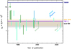Fig. 1 Synoptic presentation of measurements of the fractional Jovian deuterium abundance, as determined from HD/H2 (bright green) and CH3D/CH4 (dark green). Values for Saturn, Uranus, and Neptune are shown for comparison. Deuterium fractions in various relevant environments are given as follows (from top to bottom): terrestial (dark-blue bar), represented by the Vienna standard mean ocean water (VSMOW, Gonfiantini et al. 1995); solar-wind derived (without and with corrections for protosolar 3He), orange-hatched area; high-z (violet bar); local ISM (gray-filled area). The latter comprises determinations by Linsky (1998) and, including interstellar dust, Linsky et al. (2006). For further references see main text.

2 Method

In principle, abundance determinations for both pairs of isotopologues, HD/H₂ and CH₃D/CH₄, require a correction for isotopic exchange reactions. The deuteration of CH₄ is coupled to that of H₂ by means of the reaction CH₃ + HD ← CH₃D + H (Fegley & Prinn 1988, further references therein); it is a source for CH₃D rather than a substantial sink for HD because the latter is the by far most abundant carrier of deuterium. For CH₄ in Jupiter’s and Saturn’s atmospheres, models predict enrichment factors of $$f:=\frac{\frac{1}{4}\left[{\mathrm{C}\mathrm{H}}_3\mathrm{D}\right]/\left[{\mathrm{C}\mathrm{H}}_4\right]}{\frac{1}{2}[\mathrm{H}\mathrm{D}]/\left[{\mathrm{H}}_2\right]}=1.2$$(1)

(Fegley & Prinn 1988, the factors correct for stoechiometry). Convective motions were included by Lecluse et al. (1996) and yield f = 1.25 ± 0.12 and 1.38 ± 0.15 for Jupiter and Saturn, respectively. For the HD/H₂ pair analyzed in the present study, we assume no fractionation, that is, $$g:=\frac{\frac{1}{2}[\mathrm{H}\mathrm{D}]/\left[{\mathrm{H}}_2\right]}{[\mathrm{H}]/[\mathrm{D}]}=1.$$(2)

This choice is motivated by the result that in steady-state equilibrium of the reactions $${\mathrm{H}}_2+\mathrm{D}\rightleftharpoons \mathrm{H}\mathrm{D}+\mathrm{H},$$(3)

and at a representative temperature of 200 K, one obtains g = 1.032, adopting reaction rate coefficients from Mielke et al. (2003) and parametrized by Glover & Abel (2008).

In our observational setup (Sec. 3), the quadrupole rotational lines of H₂ used by Lellouch et al. (2001) were not available for simultaneous observations. We note that the S(1) line of ortho-H₂ at λ 17.03 μm (Roueff et al. 2019) traces the Jovian stratosphere (e.g., Lellouch et al. 2001) rather than the troposphere, while the HD, J = 1–0 line traces mainly the latter, as is shown in the following. The ground-state line of para-H₂ at λ 28.22 μm is sensitive to deeper, tropospheric layers and was mapped with the EXES instrument (Richter et al. 2018) aboard SOFIA. At that wavelength, the sensitivity of the detector fades, which requires careful calibration work left for a follow-up study (priv. comm. C. DeWitt). Because the vapor pressure curve for CH₄, as normalized with its volume mixing ratio, falls below the temperature profile of Jupiter, no CH₄ ice forms in its atmosphere (e.g., West 2014). This suggests a constant volume mixing ratio down to a pressure of 1 mbar (Sánchez-López et al. 2022). Rotationally quasi-forbidden transitions of vibrational ground-state CH₄ are a promising tracer for assessing the adopted layering (cf. Lellouch et al. 2015, for Uranus and Neptune) and for the study at hand we will address the usefulness of one of them (J = 6–5 at λ 159 μm) in appendix B.

3 Observations

The present heterodyne spectroscopy was conducted with the four-color extension 4GREAT (Duran et al. 2021) of the German Receiver for Astronomy at Terahertz Frequencies (GREAT) on one of SOFIA’s last flights with this instrument, departing from Christchurch, New Zealand, on 2022 July 13 (project id 83_0903). The 2.5-THz channel 4G4 was tuned to the rest frequency of the υ = 0, J = 1–0 line of hydrogen deuteride (HD), 2674.986094 GHz (Drouin et al. 2011), with respect to Jupiter’s barycenter. An improved solid-state local oscillator source (LO, developed by Virginia Diodes Inc., USA) was used for these nonstandard observations beyond the released frequency band of channel 4G4. While providing record power (~4 μW at that frequency), the relatively short output power required a Martin–Puplett interferometer as diplexer to couple the signal and LO beams. The LO was tuned to yield a sideband separation of 2.8 GHz, optimizing the avoidance of unwanted telluric image-band features while offering a spectral bandpass of sufficient width: The response of such a diplexer is sinusoidal, which limits the usable reception bandwidth to 1.4 GHz in the present case (3 dB roll-off in noise). A most welcome feature of the diplexer operation is that reflections in the optical path, unavoidable in heterodyne observations against a strong background source, are better suppressed in the band center, while they become more visible again in the flanks of the passband. 4G4 uses a hot-electron bolometer mixer (Pütz et al. 2012) as detector, and a digital Fourier-transform spectrometer (XFFTS, Klein et al. 2012) as backend.

At the beginning of the observations, 16:43 UTC, the velocity of the planet with respect to the observatory was 26.94 km s⁻¹, and its angular equatorial and polar diameters¹ ${42}_{.}^{\mathrm{\prime }\mathrm{\prime }}54$ and ${39}_{.}^{\mathrm{\prime }\mathrm{\prime }}78$, respectively. The planet’s north pole was at ${25}_{.}^{\circ }1$ east from north; the planetocentric latitude at the subobserver point was $2_{.}^{\circ }5$ N and its System III longitude ${245}_{.}^{\circ }7$ W. A total of 17 spectra was taken at elevations ranging from ${40}_{.}^{\circ }3$ to ${43}_{.}^{\circ }5$ with 40.4 min integration time equally shared between the planet’s disk center and a reference position 90″ east. These scans were alternated with short integrations on loads at ambient and cold temperature to convert backend count rates to Rayleigh-Jeans equivalent brightness temperatures (antenna-temperature scale). The atmospheric transmission was deduced from the measured off-target sky brightness by means of the am atmospheric model (Paine 2022), using the kalibrate module of the KOSMA software package (Guan et al. 2012) and yielded a water-vapor column of 5.7 μm (median value at zenith), resulting in single-sideband system temperatures of typically 6100 K (median, with a median receiver-noise contribution of 5860 K). These numbers refer to the ultimately used, 1.24 GHz wide portion of the approximately parabola-shaped spectral bandpass, from −80 to +60 km s⁻¹, chosen to avoid residuals of nearby telluric features.

Despite the correction of the Jovian continuum emission for telluric features, the resulting spectral baselines are not flat but characterized by higher-order polynomials, arising from the propagation of standing-wave features and post-mixing signal processing (at an intermediate frequency of 1.4 GHz). To first order these instrumental effects can be described as spectral gain variations, which can be characterized (and hence corrected) by means of a celestial target void of spectral lines, observed with exactly the same tuning parameters and Doppler correction. We therefore observed the almost full Moon (illuminated fraction 99.87%, disk diameter 2032″ at start) on a flight leg starting at 15:41 UTC (that is, preceding that of Jupiter), on which we recorded seven scans with a total integration time of 768 seconds equally shared between a position at Δα cos δ = −968″ from the center of the lunar disk (close to Mare Crisium), and a blank-sky position 90″ further west. A detailed description of the bandpass calibration can be found in Appendix A. After its application to the data, the final spectra are presented at 0.55 km s⁻¹ resolution. The radiometric noise across the bandpass is not uniform, owing to the convolution of the HEB noise with the diplexer bandpass. At the center of the diplexer response, the 1σ sensitivity is 0.11 K (Rayleigh-Jeans equivalent main-beam temperature scale), increasing to 0.34 K off-center.

Using a theoretically expected main-beam efficiency of 0.7 and the measured half-power beam width of ${10}_{.}^{\mathrm{\prime }\mathrm{\prime }}66$ (corresponding to 36 000 km on the planet’s surface), the deduced Rayleigh-Jeans equivalent brightness temperature of Jupiter at 2675 GHz amounts to 82–84 K after correcting for the 6% pickup of emission received beyond the main lobe of the instrument’s Airy pattern. For comparison, the Planetary Spectrum Generator (PSG, Villanueva et al. 2018) predicts for a distance of 4.63 AU a brightness temperature of 83 K, in excellent agreement, given the general calibration uncertainty of 10%. The corresponding Planck temperature is 137 K.

For comparison, the dayside temperature of the Moon at a selenographic position of (l, b) = (60°, 20°) of 380 K (Williams et al. 2017, Diviner lunar radiometer experiment) converts to a Rayleigh-Jeans equivalent brightness temperature of 256 K, accounting for a 20% loss due to the telescope’s central blockage and spillover, vs. 238 K measured. The difference arises from the time lapse after lunar noon at the selected selenographic position; for model fitting to Diviner measurements and further literature we refer to Vasavada et al. (2012).

4 Analysis

4.1 Atmospheric model

The temperature and number-density profiles of our atmospheric model follow Moses et al. (2005), as do the volume mixing ratios X of H, He, and CH₄. The volume-mixing ratio of H₂ is then determined as X(H₂) = 1 − X(H) − X(He) − X(CH₄), to a precision which for the paper at hand is sufficient: down to a pressure of 10⁻³ mbar, the volume-mixing ratios of the other species (atomic carbon, CH_j with j = 1, 2, 3, C₂, and C₂H) fall more than three orders of magnitude below that of CH₄. The volume mixing ratios of the ingredients of our atmospheric model (H₂, He, CH₄, NH₃, PH₃, and water- and ammonia-ice) are shown in Fig. 2. We note that the corresponding He/H₂ ratio (R, by number) of 0.158 agrees with the measurement of the Helium Abundance Detector aboard the Galileo probe (von Zahn et al. 1998, R = 0.157 ± 0.003). For the CH₄ abundance, we also apply a variant with a steeper gradient (Sánchez-López et al. 2022). Their opacity functions were obtained, on a (p, T) surface, from the PSG (Villanueva et al. 2018). For water and ammonia ice, we use absorption cross-sections from Warren (1984) and Martonchik et al. (1984), respectively, assuming a mean effective radius of 0.5 μm.

As is shown in Sec. 5.2, the predominant gaseous absorbant is ammonia. It was found by Blain et al. (2018) to be depleted in the northern equatorial belt (NEB). For our model, we refer to their demonstration of retrievals toward System III position (8° N, 215° W). Although in projection the position targeted by us ($2_{.}^{\circ }5$ N, ${245}_{.}^{\circ }7$ W) is approximately one half-power beamwidth away, it falls only ~3″ below the lower confine of the NEB (which is bounded by eastward and westward jets at 7° and 17° N, respectively; Fletcher et al. 2017, further references therein). Moreover, at the longitude observed by us the depletion of ammonia extends toward the equator. In our analysis, we will therefore adhere to retrievals yielding low NH₃ volume-mixing ratios (as an indication, 112 ppm at 2 bar). The ammonia depletion in the NEB was later confirmed by de Pater et al. (2019) and Bjoraker et al. (2022).

The abundance profile of PH₃, as a disequilibrium species, is difficult to constrain by models. Following Nixon et al. (2007) and Cavalié et al. (2023), we approximate it by an empirical layering with a constant volume mixing ratio q₀ above a threshold pressure p₀ and a power-law of the form $$q=q_0{\left(\frac{p}{p_0}\right)}^{\frac{1-f}{f}}$$(4)

below. We adopt the parameters q₀ = 6 × 10⁻⁷, p₀ = 500 mbar and f = 0.2 (Cavalié et al. 2023) for the fractional scale height. As is shown in Sec. 5.2, this particular choice has a limited impact on the analysis and abundance retrieval (unlike the layering of NH₃). We did not consider other gaseous or solid species; our omission of ammonium hydrosulfide (NH₄SH) aerosols will be commented further below (Sec. 5.2).

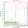Fig. 2 Vertical temperature (red) and abundance profiles against pressure altitude (ordinate), as used in the best-fit model. Abscissae (all in ppm, indicating mass fractions for ices, and volume-mixing ratios for gaseous species) are as follows: ammonia ice (green), water ice (bright blue), H2 and HD (dark blue, solid respectively dashed profile), He (medium blue), CH4 (yellow solid line, Sánchez-López et al. 2022), NH3 (orange, solid line), PH3 (orange, dotted line). The dashed yellow CH4-profile is the original abundance layering from Moses et al. (2005). For further references see Table 1.

4.2 Radiative transfer

We assume the level populations to be in local thermodynamic equilibrium (LTE). For HD, the assumption is justified, as shown by the following assessment: For 200 K gas temperature, the critical H₂ density for the J = 1 level to be populated against spontaneous decay to the ground state can be estimated to 1400 cm⁻³ (collisional rate coefficients are from Flower & Roueff 1999). As will be discussed in Sec. 5, the corresponding altitude falls well above that to which our observations are sensitive. The partitioning of H₂ into its ortho and para isomers is also assumed to be in thermal equilibrium, possibly established thanks to heterogeneous catalysis on aerosols (West 2014). This is required for an adequate description of collision-induced contributions to the total opacity (for references see Table 1).

The radiative-transfer calculations are performed in two-dimensional, cylindrical coordinates, to include the planet’s fast rotation (period 9^h55^m${33}_{.}^{\mathrm{s}}24$). Each sightline, starting at the base pressure of our model, 6.7 bar, or, for grazing sightlines, at the lower pressure boundary of 7.4 × 10⁻⁸ mbar, is decomposed into 1000 sightline segments. In each of these segments, the local emissivity at pressure level p₀ and the transmission $\mathcal{T}$(p₀) toward the outer boundary of the atmosphere model at p_out = 7.4 × 10⁻¹¹ bar are expressed as Chebyshev polynomials of order 25, which provides, through a comparison of the coefficients, an analytical solution that is as accurate as the Chebyshev approximation (for details, see Wiesemeyer et al. 2023). The transmission is related to the absorption coefficient κ(p) at pressure level p by the sightline integral $$\mathcal{T}\left(p_0\right)=\exp (-{\int }_{p_0}^{p_{\text{out }}}\kappa (p)dp).$$(5)

This technique facilitates the adaptation of the sightline sampling to abundance jumps or steep opacity gradients. The final spectra are synthesized with a channel separation of 1.0 km s⁻¹ (8.92 MHz for the HD J = 1–0 line, and 6.28 MHz for the CH₄ 6–5 line), and convolved into a main beam of ${10}_{.}^{\mathrm{\prime }\mathrm{\prime }}7$ (half-power width). Internally, the code uses a 0.5 km s⁻¹ spectral resolution. A spectrum obtained for 0.25 km s⁻¹ internal sampling showed no noticeable difference from the original one (0.25‰ relative to the continuum level), thanks to the semi-analytical convolution, invariant against spectral discretization, of thermal and pressure-induced line broadenings. We will see hereafter that the widths of both contributions equalize at 25 mbar, where the temperature amounts to 140 K and the corresponding thermal broadening to 1.47 km s⁻¹ (FWHM). Our model accounts for single-forward scattering of solar photons by the ice particles and resonant scattering by HD, but finds it neglectable at our far-infrared wavelengths. Likewise, the inclusion of zonal winds (Tyler 2022) leads to no noticeable distortion of the shapes of the beam-convolved model spectra. Even the largest sightline-projected wind speeds of 360 m s⁻¹, occurring in the southern polar region (Cavalié et al. 2021), are immeasurable at the sensitivity of our data.

Thanks to its high spectral resolution, our study is sensitive to a thorough description of the pressure-induced line broadening and shift. Here we apply two different approaches. The first one expresses the half-maximum half-width (HMHW) γ_L of the Lorentz profile of the opacity coefficient in a parametrized form, $${\gamma }_{\mathrm{L}}(p,T)=p\cdot {\gamma }_{\mathrm{L},0}\left(T_0\right)\cdot {\left(T_0/T\right)}^{\mathrm{n}},$$(6)

where γ_L,0, usually expressed in cm⁻¹ /atm, is the Lorentz HMHW for a pressure of 1 atm and at a reference temperature T₀ (usually 296 K). The temperature dependence of γ_L is expressed as a power law with exponent n; for example, in the hard-sphere approximation and for an ideal gas it takes the value n = 0.5. The pressure-induced line shift δ is parametrized as $$\delta (p,T)=p\cdot ({\delta }_0\left(T_0\right)+{\delta }^{\mathrm{\prime }}\cdot (T-T_0)),$$(7)

where δ₀ is the line-center shift (in cm⁻¹) at 1 atm and 296 K, to which is added a linear temperature dependence, described by a gradient δ′. The resulting rest-frame line profile is convolved with a Maxwellian velocity distribution at the ambient temperature T, yielding a Voigt profile (for a fast numerical convolution, a rational approximation to the Voigt function was used, Humlícek 1982). For collisions with H₂, Sung et al. (2023) determined the above parameters experimentally at a range of relevant temperatures and pressures.

In a more sophisticated approach, the explicit velocity dependence of the Voigt profile is taken into account. Stankiewicz et al. (2021) provide a parametrized form for the velocity-averaged pressure broadening and shift coefficients of the collisional HD–He system, γ₀ and δ₀ along with the coefficients γ₂ and δ₂ for a second-order approximation in speed, such that $$\gamma (v)+i\delta (v)\simeq {\gamma }_0+i{\delta }_0+({\gamma }_2+i{\delta }_2)({\left(\frac{v}{v_{\mathrm{m}}}\right)}^2-\frac{3}{2})$$(8)

where υ_m is the most probable speed at the local gas temperature T. The parametrization of the temperature dependence of γ_0,2 and δ_0,2 is either given in the forms $$\begin{array}{rl}& {\gamma }_{0,2}(T)=g_{0,2}{\left(T_{\mathrm{r}\mathrm{e}\mathrm{f}}/T\right)}^{n,j}+g_{0,2}^{\mathrm{\prime }}{\left(T_{\mathrm{r}\mathrm{e}\mathrm{f}}/T\right)}^{n^{\mathrm{\prime }},j^{\mathrm{\prime }}}\\ & {\delta }_{0,2}(T)=d_{0,2}{\left(T_{\mathrm{r}\mathrm{e}\mathrm{f}}/T\right)}^{m,k}+d_{0,2}^{\mathrm{\prime }}{\left(T_{\mathrm{r}\mathrm{e}\mathrm{f}}/T\right)}^{m^{\mathrm{\prime }},k^{\mathrm{\prime }}}\end{array}$$(9)

or explicitly tabulated as a function of temperature (for practical purposes, for γ_0,2 and δ_0,2 we use interpolating polynomials of sixth and ninth order in ln T, respectively). Dicke narrowing (Dicke 1953) was included in our line profile modeling using a similar parametrization, but showed no effect that would be distinguishable at the sensitivity of our data.

Equipped with this parametrization, we used the qSDV subroutine (Ngo et al. 2013; Tran et al. 2013) for the efficient numerical calculation of the quadratic speed-dependent Voigt profile. For the second collision partner (He in the first approach, and H₂ in the second one) we also use the above prescriptions but apply scaling factors deduced from older work; for details we refer to Fig. 3 and references therein. For the first approach (that is, pressure-shifted Voigt profiles), the corresponding pressure-altitude profile of the line broadening and -shift is shown in Fig. 4.

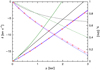Fig. 3 Pressure broadening γ (solid lines and dots, right ordinate) and shift δ (dashed lines and crosses, left ordinate) below 3 bar: HD-H2 for experimentally determined parameters (black, Sung et al. 2023, ≤ 1 bar) and calculated ones (green, Schaefer & Monchick 1992, for equilibrium ortho/para mixture). HD-He (theoretical) from Thibault et al. (2020, magenta), Schaefer & Monchick (1992, blue), and Stankiewicz et al. (2021, red).

5 Results and discussion

The observed HD (1–0) line is shown in Fig. 5, together with fits resulting from the parametrizations of the line profile as described in the previous section (for the same spectrum prior to the bandpass calibration see Appendix A and Fig. A.1). The best-fitting synthetic spectrum has a normalized χ² = 1.14 and generates a continuum level of 87 K (Rayleigh-Jeans equivalent main-beam brightness temperature). In the following, we first discuss the results in view of the pressure-induced line broadening and shift, followed by a discussion on the impact of the assumed atmospheric layering on the HD line profile and the derived deuterium fraction and its global uncertainty.

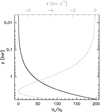Fig. 4 Pressure altitude vs. ratio of pressure and thermal broadening (lower abscissa, solid line) and pressure-induced line shift (dashed gray, upper abscissa) as used in Sec. 5.1.

5.1 Beyond-Voigt line profiles

Using the experimentally determined line-broadening parameters from Sung et al. (2023, SOLEIL synchrotron source) for HD–H₂ collisions (and empirically scaling them to those for the HD–He system) yields a decent description of the line profile in terms of the overall line-shape including the asymmetry between the predominant absorption feature and the weak stratospheric emission feature at line center. The latter actually coincides with the sightline-projected velocity of Jupiter with respect to the observer, while the absorption is blue-shifted, as expected from the experimental findings obtained at the SOLEIL facility. As a caveat, we note that the radio-metric noise is not constant across the spectrum. This results from the injection of the local oscillator signal through a Martin–Pupplet interferometer (required for high throughput and thus sufficient power, for details see Sec. 3), leading to a noise bandpass with an approximately parabolic shape whose depth results from the trade-off between sensitivity and exploitable bandwith. Consequently, the system temperatures (and hence radiometric noise) on the usable, line-free baseline are a factor of typically 1.4 higher than across the line profile. We further account for the aforementioned standing-wave suppression by the diplexer (Sec. 3), which is more efficient at line center than outside where it is imperfectly removed by the bandpass calibration. Scaling the normalized χ² values (variance of the residuals with respect to that of the baseline noise) upward by a factor of 1.64² ≃ 2.7 yields for the model applying pressure-shifted Voigt profiles the expected χ² close to unity and from now on serves as reference. The best-fitting profiles are indeed those that account for the pressure-induced line shift; for quadratic speed-dependent Voigt profiles we obtain χ² = 1.6. We note that this figure can be improved by a parametrization of the collisional broadening of the HD/ortho-H₂ and HD/para-H₂ systems, equivalent to that of the HD–He system (Stankiewicz et al. 2021), rather than empirically scaling published results to the H₂/He mixture at hand. We discard the simple pressure-broadened Voigt profile (χ² = 2.0) as inadequate, owing to its symmetry. On the other hand, while an asymmetric line profile is a necessary condition for the presence of pressure-induced line shifts, it is not sufficient because it can also be produced by the planet’s rotation in response to a mispointing (±2″ cannot be excluded). We note, however, that only an unlikely mispointing of −4″ can reproduce the observed asymmetry, but it would also shift the line profile redward by an untolerable velocity offset of 3 km s⁻¹, which results in a significantly increased χ² = 7.1 (Fig. 5). We therefore conclude that the pressure-induced line shift is the most likely explanation for the observed asymmetry. Even in the unlikely case that the latter was caused by the planet’s fast rotation and instrumental errors, the impact on the derived deuterium fraction would be at the ~1% level, well within the uncertainties estimated in the next section. Ultimately, only a fully sampled map of the HD line can resolve the ambiguity. Such an observation would also provide valuable constraints on the assumed layering because the nature of the line profile changes significantly toward Jupiter’s limb, a phenomenon that we will discuss hereafter.

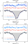Fig. 5 HD (J = 1–0) spectrum toward Jupiter’s center, with best-fit models overlaid. The velocity scale refers to the Jovian system baryceter. Top: HD (J = 1–0) (black line and gray-filled histogram) and modeled Voigt profiles with pressure shift (red) and without (blue, the dashed profile is for a $-4_{.}^{\mathrm{\prime }\mathrm{\prime }}2$ pointing offset). Residuals and their normalized χ2 values (in brackets for the offset pointing) are shown atop (in corresponding colors, with ordinate shifts for clarity). Note the less-suppressed bandpass ripples located on the wings of the absorption profile, as discussed in section 3. Bottom: as above, but comparing the speed-dependent with the pressure-shifted Voigt profile (blue, respectively red).

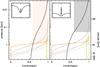Fig. 6 Profiles of the transmission in the HD, J = 1–0 line for sight-lines originating at the sub-observer point (left) and shifted along the equator to a projected distance of 0.75 Jupiter radii (${15}_{.}^{\mathrm{\prime }\mathrm{\prime }}95$), $5_{.}^{\mathrm{\prime }\mathrm{\prime }}3$ from the planet’s limb (right). The inserts show synthesized spectra for these sightlines at the same scales of (−60, +60) km s−1 and (1.4, 2.2) kJy/beam. For demonstration purposes, the spatial resolution was increased (2″ half-power width, for Nyquist-critical 1″ sampling steps) and the planet’s rotation omitted. The abscissa represents the sightline transmission $\mathcal{T}$ from a pressure altitude p0 (left ordinate, the right ordinate shows the corresponding altitude above a 6.7 bar base level) to pout toward the observer, related to the absorption coefficient κ by equation (5), with contributions from HD, J = 1–0 (black, at line center), collision-induced absorption (due to H2−H2 collisions, solid gray, and H2−He collisions, dashed gray), bright-blue (water ice), green (ammonia ice), CH4 (yellow), NH3 (orange), and PH3 (dashed orange). The color assignment is identical to that in Fig. 2. The crossings of each curve with the lower abscissa indicate the transmission from the base to the top level of the model atmospheres for the given solid or gaseous species. The area where the transmission along the sub-observer sight-line is limited by self-absorption in HD ($\mathcal{T}$self), rather than by the NH3 opacity, is highlighted in beige (left). For the off-center sightline, the gray area indicates the pressure range for which the transmission falls above $\mathcal{T}$self (right).

5.2 Layering, opacities, and resulting HD abundance

The main agents impacting the radiative transfer of the HD (1–0) line are CH₄, NH₃, and PH₃ for the gaseous species, and H₂O and NH₃ for the ices (their abundance profiles are shown in Fig. 2). Owing to the lack of optical constants of solid ammonium hydrosulfide (NH₄SH), located between the water- and ammonia-ice layers in the 1 −2 bar pressure interval (Zuchowski et al. 2009), we do not account for its absorbance, which for the study at hand is of minor importance: The major contributor to the λ 112 μm absorbance is gaseous NH₃; only at pressures below 800 mbar it is surpassed by the absorption induced by collisions among H₂ molecules, yet allowing for a transmission of at least 67%. Figure 6 shows these transmissions as a function of the pressure footpoint, and demonstrates that the observed HD (1–0) line, which is optically thin (τ < 0.6) at all pressures considered by the model (p ≤ 6.7 bar), is sensitive to pressures below typically one bar.

For the best-fit model summarized in Table 1, the deduced D/H fraction amounts to y_D = 1.9 ± 0.4. The standard deviation comprises random and systematic errors. The former arises from the spectral baseline noise, σ_rms /T_c = 0.01, which converts to σy_D ≃ 0.1 (as deduced by means of a Monte-Carlo simulation). The variation of model parameters (within reasonable limits) as discussed below yields y_D = 1.6 to 2.2. Uncertainties regarding the telluric transmission or the coupling efficiency of the telescope optics (as illuminated by the scientific instrument) are irrelevant as long as they affect line and continuum in equal measure. Owing to the lack of a dedicated calibration of the gain ratio between the signal and image band of the heterodyne receiving system (difficult to perform), we admit a ±5% deviation from the ideal case where signal and image band contribute equally to the received total power (the estimate holds for the mixers of HIFI band 7, which are equipped with hot-electron bolometers, like upGreat, Kester et al. 2017). The resulting deuterium fractions range again from y_D = 1.6 to 2.2. The indicated global error is then approximated by adding these uncertainties in quadrature.

Shifting the pressure scale for the volume mixing ratios of the gaseous species (CH₄, NH₃, and PH₃) downward by 20 mbar entails a change in the best-fit derived D/H fraction of Δy_D = +0.3, but overestimates the stratospheric emission feature at the line center. The normalized χ² therefore increases from 1.1 to 1.3, while the continuum level decreases slightly from 87.8 to 85.2 K (Rayleigh-Jeans equivalent main-beam brightness temperature). This behavior can be explained by the increased opacity blocking the deeper layers with a negative temperature gradient, producing the prominent absorption. Conversely, shifting the pressure scale upward by 20 mbar decreases the best-fit deuterium fraction by Δy_D = 0.2, significantly underestimates the stratospheric emission feature (entailing a χ² = 1.8) and yields a continuum level of 90.5 K. In a scenario with an enhanced CH₄ abundance (Sánchez-López et al. 2022), the resulting best-fit deuterium fraction still amounts to y_D = 1.9 (χ² = 1.14, T_c = 87.0 K); as shown in Fig. 6, the contribution of the CH₄ bands to the broadband opacity at λ 112 μm, compared to that of NH₃, is of minor importance, with a transmission of 96% along the whole sightline considered by the best-fit model (base-pressure level 6.7 bar). In contrast, a 10% increase of the NH₃ abundance would require a deuterium fraction of y_D = 2.2 to explain the observed line profile, while reproducing a continuum level of 87 K. Despite a similar χ², with such a modification both the stratopheric emission component and the absorption depth are slightly overestimated (using pressure-shifted Voigt profiles). A 10% lower NH₃ abundance, with a deuterium fraction of y_D = 1.9, fits the absorption profile but under-predicts the emission component. The upwelling of the disequilibrium species PH₃ (Giles et al. 2015) could in principle add another uncertainty. However, as we show in Fig. 6, the formation of observable lines is impeded by PH₃ only at pressures above typically 2 bar, where the opacity due to NH₃ is the dominating agent.

For a good recovery of the continuum level, we apply a scaling factor to the cross-sections of the ice opacities for 1.0 μm large particles (effective size). This choice does not come without its rationale; it allows us to implicitly consider the presence of aerosols otherwise unaccounted for (e.g., NH₄SH) and reflects uncertainties related to the size distribution of the ice particles. The λ44 μm water-ice feature measured on the Voyager 1 and 2 flybys could be fit by 2 μm-sized particles (Simon-Miller et al. 2000), which barely changes the extinction coefficient compared to that of the half-sized particles used by us. However, for NH₃ ice, Orton et al. (1982) estimate lower size limits of 3 to 10 μm, depending on the underlying vertical particle distribution. Using the latter values instead of 1.0 μm increases the extinction coefficient at λ112 μm by a factor 1.7. For the stratosphere, more recent studies predict particle sizes of 0.3 to 0.6 μm at 100 mbar (López-Puertas et al. 2018; Anguiano-Arteaga et al. 2021). The line-profile fits shown in Fig. 5 were obtained by doubling the ammonia- and water-ice opacities (Martonchik et al. 1984; Warren 1984, respectively). It is plausible that the excess opacity required to reproduce the λ 112 μm continuum is provided by aerosol particles which on global average play an important role in the thermal balance of the middle atmosphere (at pressures of order 10 mbar); at around λ 100 μm, the imaginary parts of the complex refractive indices of aerosols in simulated and observed atmospheres differ by a factor two (Zhang et al. 2015, further references therein). The nominal values result in a lower opacity and therefore make the line profile sensitive to warmer layers. Consequently, the continuum level rises slightly to 89 K, while the line profile fit would require a deuterium fraction as low as y_D = 1.8. Increasing the ice opacity by a factor three with respect to the above references restores the best-fit y_D = 1.9 and decreases the continuum level insignificantly to 86.5 K, but starts to over-estimate the stratospheric emission component at line center, resulting in a suboptimal fit (χ² = 1.5).

We emphasize that the prominence of the narrow stratospheric emission feature mainly depends on the characteristics of the layering of gaseous NH₃. Thanks to the aforementioned depletion of the latter in the equatorial regions, the HD absorption traces lower tropospheric layers and therefore deepens. The kernel of its Voigt-like profile is narrow because the self-absorption in the HD (J = 1–0) line is mild (Fig. 6). A similarly narrow stratospheric emission feature fills this kernel, making it flatter, but does not exceed the continuum level. As shown in Fig. 6 (right panel), owing to the inclination of the sight-line with respect to the surface normal, at ${15}_{.}^{\mathrm{\prime }\mathrm{\prime }}95$ equatorial offset (0.75 Jupiter radii) the transmission due to NH₃ drops below 10% already at 1.0 bar pressure (and further out, at only 1″ from the planet’s limb, at 0.85 bar), rather than 1.1 bar for the sightline to the sub-observer point (left panel). As expected and demonstrated in Fig. 6, the HD emission starts to dominate the absorption because the blockage of deeper layers, producing the prominent absorption, favors the stratospheric contribution to the line formation. The resulting line shapes are shown in Fig. 7 (top); on the off-center positions 85% of the main-beam area still couples to the disk. Such an observation will also facilitate a refined analysis of the pressure-induced line shift: For a given Jovian latitude, the differential spectrum between two opposite longitudes would be strictly antisymmetric (with respect to the planet’s systemic velocity) only in absence of such a line shift and of local variations of the NH₃ abundance. As shown in Fig. 7 (bottom), the resulting line profile is asymmetric and not antisymmetric; pointing errors, if present, can be mitigated by comparing the continuum levels on either position. At the sensitivity of our observations (see section 3), this subtle feature, of 0.65 K (Rayleigh-Jeans equivalent main-beam temperature), would have been detectable. We also note that at higher spatial resolution, even toward the sub-observer point the emission feature will become more pronounced (yet without exceeding the continuum level), because the main-beam pickup of rotational broadening will be gradually suppressed. At 2″ half-power beamwidth and on that sightline, the model spectra with and without rotation are barely distinguishable (cf. Fig. 6, inserts). This demonstrates in particular that the weakness of the stratospheric emission component (with respect to the depth of the absorption feature) is not due to beam- and rotation-smearing, neither to a small mis-pointing, leaving the layering of broadband absorptions as only explanation. By the same token, the absorption components of spectra taken toward polar latitudes with their presumably higher NH₃ abundance may be expected to weaken, which would push the emission feature there even more above the continuum level.

In summary, the changes of the best-fitting deuterium fractions entailed by variations of the adopted layering stay within the global error estimated above. In order to confirm the subtlety of the interplay of tropospheric absorption and stratospheric emission, and to exclude a potential risk of unresolved ambiguities, we apply our model layering to another species, CH₄. To date, its tropospheric volume mixing ratio is assumed to be constant, whereas the stratospheric profile and in particular its potential variability is not yet conclusively characterized (Moses et al. 2005; Sánchez-López et al. 2022, further references therein). As we will show in Appendix B, the J = 6–5 line of the molecule’s vibrational ground state does not suffer from strong self-absorption because it is zero-order rotationally forbidden; its absorption component is therefore sensitive to the tropospheric layering and coincides with the pressure interval in which the HD (J = 1–0) line forms.

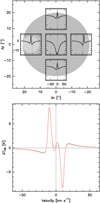Fig. 7 Synthetic HD (J = 1–0) spectra. Top: five-point cross sampled at ${15}_{.}^{\mathrm{\prime }\mathrm{\prime }}95$ distance, against the gray-shaded Jupiter disk. The vertical axis coincides with the planet’s sky-plane projected rotation axis. All spectra have the same ordinate range (in K on Tmb scale) and are continuum-subtracted for clarity. The white-hatched circle centered at offset (${15}_{.}^{\mathrm{\prime }\mathrm{\prime }}95$, $0_{.}^{\mathrm{\prime }\mathrm{\prime }}0$) displays the half-power beam width of the observations. The systemic velocity is marked by vertical dotted lines. Bottom: differential spectrum between offsets ($+{15}_{.}^{\mathrm{\prime }\mathrm{\prime }}95,0_{.}^{\mathrm{\prime }\mathrm{\prime }}0$) and ($-{15}_{.}^{\mathrm{\prime }\mathrm{\prime }}95,0_{.}^{\mathrm{\prime }\mathrm{\prime }}0$) (red). The equivalent spectrum without pressure-induced line shift (gray) is shown for comparison.

6 Conclusions

We observed and analyzed the profile of Jupiter’s HD (J = 1–0) line toward System III position ($2_{.}^{\circ }5$ N, ${245}_{.}^{\circ }7$ W) at ${10}_{.}^{\mathrm{\prime }\mathrm{\prime }}66$ halfpower beam width and with high spectral resolution. The line profile is dominated by a tropospheric absorption feature, partially filled by stratospheric emission. The deduced deuterium fraction amounts to (19 ± 4) ppm (y_D = 1.9 ± 0.4), bringing it into agreement with that of Saturn (Lellouch et al. 2001), both falling a factor of about three below the deuterium fractions of Uranus and Neptune (Feuchtgruber et al. 2013). We cannot confirm the finding of Pierel et al. (2017) that Saturn harbors a significantly lower deuterium fraction than Jupiter. Our data suggest that both atmospheres are equally well suited to diagnose the deuterium fraction of the protosolar nebula. The global uncertainty of our value compares with that of the deuterium fraction inferred from solar-wind measurements (Geiss & Gloeckler 1998) and leaves both studies in peaceful coexistence. Notably, a recent PACS study of the HD (J = 1–0) line obtains a deuterium fraction (15 ± 6) ppm (Gapp et al. 2024) and comes to the same conclusion. While both measurements agree within their uncertainties, the lower PACS value might be a consequence of the spectrally unresolved stratospheric emission component if interpreted as reduced tropospheric absorption.

The stratospheric emission component is centered at the systemtic velocity, while the absorption profile underneath is shifted to a slightly higher frequency, introducing an asymmetry in the line profile. This agrees with recent measurements of the pressure-induced line shift of the rotational spectrum of HD (Sung et al. 2023) and is also predicted by speed-dependent beyond-Voigt profiles (e.g., Stankiewicz et al. 2021, further references therein). Our line-profile modeling also shows that the response of a slight mispointing to the planet’s fast rotation is unlikely to cause the observed asymmetry. A fully-sampled map of Jovian HD lines would not only dispel such concerns, but also help further constraining the abundance profiles across the atmosphere or reveal zonal variations. This holds in particular for the impact of the opacity of the ammonia bands. For the HD (J = 1–0) line and a previously observed, rotational line of CH₄ (J = 6–5, arising in the vibrational ground state), these bands block the atmospheric transmission at pressures of typically 1 bar. The different depths of the NH₃ absorption bands at λ 112 μm and λ 159 μm are decisive in shaping the emergent line profiles (the CH₄ line is dominated by stratospheric emission, unlike the HD line). Toward the limb of Jupiter, this opacity barrier is reached at lower pressure, which is why the stratospheric emission feature there dominates the spectrum, even for the HD line. We demonstrated that at the radiometric sensitivity reached by our experiment and using the Moon as a bandpass calibrator, a fully sampled map of Jupiter would have been entirely feasible for upGreat aboard SOFIA, providing important clues on the atmosphere’s vertical layering (through the limb-darkening effect) and on local variations of its main absorbants. We recommend it for execution by balloon-borne or future space missions (e.g., OASIS, Anderson et al. 2022) dedicated to high-resolution far-infrared spectroscopy.

Acknowledgements

We owe the observatory staff a debt of gratitude; their commitment to the project was indispensable for the execution of these demanding observations. We made use of the Planetary Spectrum Generator, providing us with valuable support, and thank its P.I. Geronimo Villanueva and the participating team not only for the development work, but also for making the tool available to the community. We thank Virginia Diodes Inc. for their continuous efforts to improve the performance of the 2.7 THz local oscillator source, which made the success of this experiment possible. We thank the anonymous referee for an insightful review. Miram Rengel (Max Planck Institute for Solar System Research, Göttingen, Germany) gave valuable advice on aerosol opacities. We also thank Ankit Rohatgi for the WebPlotDigitizer (Rohatgi 2022) and for creating an intuitive access to its use. GREAT is a development by the MPI für Radioastronomie and the KOSMA/Universität zu Köln, in cooperation with the DLR Institut für Optische Sensorsysteme. The development of the instrument is financed by the participating institutes, by the German Aerospace Center (DLR) under Grants 50 OK 1102, 1103, and 1104, and within the Collaborative Research Centre 956, funded by the Deutsche Forschungsgemeinschaft (DFG). SOFIA is jointly operated by the Universities Space Research Association, Inc. (USRA), under NASA Contract No. NAS2-97001, and the Deutsches SOFIA Institut (DSI) under DLR Contracts No. 50 OK 0901 and No. 50 OK 1301 to the University of Stuttgart.

Appendix A Bandpass calibration

The calibration of the raw data follows the standard scheme in which the difference spectrum from the on- and off-position is normalized by the corresponding signal from calibration loads at ambient and cold temperature, such that $$\mathbf{R}=(T_{\mathrm{R}\mathrm{J},\text{ amb }}-T_{\mathrm{R}\mathrm{J},\text{ cold }})\cdot ({\mathbf{P}}_{\mathrm{o}\mathrm{n}}-{\mathbf{P}}_{\text{off }})\oslash ({\mathbf{P}}_{\mathrm{a}\mathrm{m}\mathrm{b}}-{\mathbf{P}}_{\text{cold }})$$(A.1)

where R denotes the reduced spectrum, P_on and P_off the power count rates received from the target and the blank sky, respectively (averaged over an integration time well below the charateristic times for instrumental and atmospheric drifts), and P_amb and P_cold those received from the warm, respectively cold loads. T_RJ,amb and T_RJ,cold are the corresponding Rayleigh-Jeans equivalent temperatures. We note that in the above equation, the signals R and P (indices suppressed for brevity) are to be understood as vectors, whose elements represent the signals in the spectral channels. The symbol ⊘ on the right-hand side of eq. A.1 represents a Hadamard (that is, element-wise) division.

Eq. A.1 is linear in ΔP = P_on − P_off, and suggests that an intrinsic (that is, perfectly gain-calibrated) spectrum ΔS = S_on − S_off can be written as $$\mathrm{\Delta }\mathbf{P}={\mathbf{g}}_1\odot \mathrm{\Delta }\mathbf{S}+\mathbf{n},$$(A.2)

where ⊙ denotes a Hadamard product, and n the noise contribution. However, in practice the mixer response is not fully linear, which for the detection of weak lines superposed on a strong continuum is a severe nuisance (Fig. A.1, top panel, cf. discussion in Cordiner et al. 2023), while standing-wave features building up between the mixer and the secondary mirror can be mitigated by nod-and-chop techniques and use of Lomb-Scargle periodograms (Cordiner et al. 2022). In the following, we present a second-order correction method. For that purpose the linear ansatz (Eq. A.2) is extended as follows: $$\mathrm{\Delta }\mathbf{P}={\mathbf{g}}_1\odot (\mathrm{\Delta }{S}_{\mathrm{c}}\cdot \mathbf{1}+\mathrm{\Delta }{\mathbf{S}}_{\ell })+{\mathbf{g}}_2\odot {(\mathrm{\Delta }{S}_{\mathrm{c}}\cdot \mathbf{1}+\mathrm{\Delta }{\mathbf{S}}_{\ell })}^2+\mathbf{n}.$$(A.3)

For reasons that will soon become clear, the spectrum is decomposed into the contributions from the continuum and the spectral (emission or absorption) line, ΔS_c and ΔS_ℓ, respectively. ΔS_c is a scalar quantity. g₁ can be determined from a load calibration via eq. A.1, $${\mathbf{g}}_1=\frac{{\mathbf{P}}_{\mathrm{a}\mathrm{m}\mathrm{b}}-{\mathbf{P}}_{\mathrm{c}\mathrm{o}\mathrm{l}\mathrm{d}}}{T_{\mathrm{R}\mathrm{J},\mathrm{a}\mathrm{m}\mathrm{b}}-T_{\mathrm{R}\mathrm{J},\mathrm{c}\mathrm{o}\mathrm{l}\mathrm{d}}}$$(A.4)

and yields the reduced (that is, first-order gain corrected) spectrum R = ΔP ⊘ g₁ (Eq. A.1). The gain vector g₂ for the second-order contribution requires an additional calibration signal void of spectral lines, recorded with exactly the same receiver tuning and spectral setup as the spectrum of Jupiter, such as the thermal emission from lunar regolith, as in the work at hand. We then dispose of measurements R_J and R_M toward Jupiter, respectively the Moon. Their continuum brightness levels are simply related by a linear scaling between two scalars, ΔS_M = αΔS_J,c.

It is then relatively straightforward to show that for the linefree spectral channels $${\mathbf{R}}_{\mathrm{M}}=\alpha \mathrm{\Delta }{S}_{\mathrm{J},\mathrm{c}}(1-\alpha )\mathbf{1}+{\alpha }^2{\mathbf{R}}_{\mathrm{J},\mathrm{c}}.$$(A.5)

The linear regression of R_M against R_J,c then yields the ordinate offset αΔS_J,c(1 − α) and slope α² as shown in Fig. A.2, allowing us to construct a line-free baseline B via $$\mathbf{B}=\frac{1}{{\alpha }^2}\cdot ({\mathbf{R}}_{\mathrm{M}}-\alpha \mathrm{\Delta }{S}_{\mathrm{J},\mathrm{c}}(1-\alpha )\mathbf{1}),$$(A.6)

such that R_J/B becomes flat and its continuum normalized to unity. The line-to-continuum ratio and the noise-to-continuum ratios, as given by the original spectrum R_J, are preserved, but compromised to a much lesser degree by higher-order spectral gain fluctuations. As a matter of fact, the baseline noise (standard deviation of line-free continuum), normalized by the continuum, amounts to 0.05 under a first-order and to 3.7 · 10⁻³ under a second-order gain correction (that is, decreased by an order of magnitude, see Fig. A.1, top and center panels). A 10% improvement in the final noise figure can be achieved by replacing B by a wavelet fit of order 8, thus suppressing the radiometric noise in the baseline spectrum.

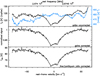Fig. A.1 Bandpass-calibration steps. Top: single-sideband calibrated spectra of Jupiter and the Moon (blue), tuned to the HD, J = 1 − 0 line and scaled in forward-beam brightness temperatures. Center: Bandpass-calibrated spectrum (normalized to unity), using the correlation shown in Fig. A.2. Bottom: After correction for atmospheric transmission and scaled to main-beam brightness temperature (Tmb, line-to-continuum ratio corrected for double-sideband reception).

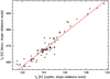Fig. A.2 Correlation between forward-beam antenna temperatures (TA, prior to atmospheric transmission correction, on single-sideband scale) for the Moon and, at an identical spectral sampling, Jupiter.

In the last step of this correction, we remove the image-band contribution from the gain-corrected spectrum, and scale the result back to Jupiter’s continuum level, T_J,c, as obtained from a dedicated double-sideband calibration. This yields the final spectrum S_J,2 (the subscript denotes the second-order gain correction), $${\mathbf{S}}_{\mathrm{J},2}=T_{\mathrm{J},\mathrm{c}}\cdot (2{\mathbf{R}}_{\mathbf{J}}\oslash \mathbf{B}-\mathbf{1})$$(A.7)

(Fig. A.1, bottom panel, and Fig. 5). The factor 2 is justified because for the HD (J = 1 − 0) line the atmospheric transmissions in the signal and image bands differ by only 1.5%, which is well within the uncertainties of the calibration and of the deduced deuterium fraction, discussed in sections 3 and 5.2, respectively.

Appendix B Spectroscopy of the CH₄ υ = 0, J = 6 → 5 line

As discussed in section 4, our retrieval of the sightline-averaged D/H ratio would benefit from an independent verification in addition to the reproduction of the monochromatic continuum level. The in situ measurements of the Galileo probe yielded a CH₄ abundance of (2.1 ± 0.4) × 10⁻³ for pressure levels of 0.5 to 8.6 bar (Niemann et al. 1998). Gladstone et al. (1996) presented a detailed photochemical model for the stratosphere, later refined by Moses et al. (2005) thanks to data from the Infrared Space Observatory, and by Sánchez-López et al. (2022) using updated reaction-rate coefficients. As mentioned in section 2, the absence of methane ice suggests a constant tropospheric volume mixing ratio of gaseous CH₄. The far-infrared, rotational ground-state lines of the latter provide a tracer for the tropospheric layering which thanks to the molecule’s small but permanent dipole moment is free from strong self-absorption. We therefore observed in addition to the HD (J = 1 − 0) line the multiplet of the purely rotational J = 6 − 5 line of CH₄ at 1881.98 GHz.

B.1 Observations

The observations were performed with the upGREAT array on a northern hemisphere flight on 2017 June 15, departing from Palmdale (Ca). upGREAT is a seven-pixel heterodyne array (Risacher et al. 2018), operating in low- and high-frequency bands at 1.83 − 2.07 THz (LFA) and 4.78 THz (HFA), respectively. The LFA used here is equipped with dual-polarization mixers; for the CH₄ line we used the horizontal polarization. The data calibration follows the same steps as for the HD J = 1 − 0 observations, up to one exception: Making use of the 60″ wide field-of-view of the array, the contribution of the sky background was removed by switching between the central and an off-center pixel, separated by ${30}_{.}^{\mathrm{\prime }\mathrm{\prime }}3$, such that the sub-observer point was always covered by a pixel. The resulting reward of a factor $\sqrt{2}$ increase in sensitivity was only compromised by a 3% beam (15″ half-power width) pickup of Jupiter’s continuum emission in the off position. The central pixels of the dual-polarization LFA targeted the sub-observer point at a planetocentric latitude of $2_{.}^{\circ }7$ S and a System III longitude of ${254}_{.}^{\circ }5$ W. The J = 6 − 5 line was detected in stratospheric emission, at 10 σ_rms (for 0.6 km s⁻¹ spectral channel spacing), on top of a broad, weaker absorption of 4σ_rms, forming in the troposphere (Fig. B.1). In view of the baseline quality, this absorption component is less well constrained. The consistency between the spectra provided by the two pixels was confirmed by means of a correlation analysis. We furthermore note that the rotational CH₄ line was also detected by the HIFI instrument (as part of the Herschel Observing Key Programme “Water and Related Chemistry in the Solar System”, Hartogh et al. 2009). Despite its lower sensitivity (5σ_rms for the emission component, while the absorption component remains undetected), this observation corroborates our finding. It was performed 1731.8 d before ours. Owing to its stratospheric origin, the emission component is prone to variability, originating in the thermal quasi-quadrennial oscillation, which was recently located in the 2 − 17 mbar region by Cosentino et al. (2017) and Giles et al. (2020). The latter study determined the period of the equatorial temperatures at 13.5 mbar to 4.0 ± 0.2 Earth years between 2012 and 2017, covering the epochs of our observations. We note the time lapse between the latter corresponds to 1.2 periods, coincidentally equalling that between our CH₄ and HD observations with SOFIA. In the following we will show that qualitatively these CH₄ observations are a useful complement for the analysis of our HD spectroscopy. Because the temperature of Jupiter’s troposphere is set by convective equilibrium with the planet’s internal heating, the absorption components of the studied CH₄ and HD lines are unlikely to undergo decadal variations.

The observations from both observatories were calibrated to main-beam brightness temperatures (with forward efficiencies of η_ff = 0.96 and 0.97 for HIFI and upGreat, respectively, and beam efficiencies of η_mb = 0.57 and, respectively, 0.68). The upGREAT data were corrected for a mean atmospheric transmission of 70% (at zenith).

B.2 Analysis and discussion

The existence of a permanent rotational CH₄ spectrum of a tetrahedral molecule such as CH₄ is a natural consequence of the frame distortion effect (Kazakov 2023, further references therein). Owing to Coriolis interaction, out of the nine vibrational modes, two (at band head wave numbers ν₃ = 3019.2 cm⁻¹ and ν₄ = 1310.8 cm⁻¹, corresponding to λ3.3 μm and λ7.6 μm, respectively) couple to the vibrational ground state, inducing there a distortion dipole moment of 23 μD. Kazakov (2023) compares theoretical determinations with laboratory measurements (Wishnow et al. 2007), yielding satisfactory agreement. The rest frequency used by us, 1881980 MHz (62.7761 cm⁻¹, Tab. B.1), was adopted from Yurchenko et al. (2024). The calculated line-profile integrated absorption coefficient (Kazakov 2023) of 1.98 × 10⁻⁵ cm⁻¹ (for a temperature of 113.5 K and a density of 2.61 amagat) agrees with our thermal-equilibrium value within satisfactory 2.8 %, using the Einstein coefficients from Yurchenko et al. (2024) and the partition function of Gamache et al. (2017). A weak telluric ozone (ν₂ = 1) absorption feature arising in the image band continuum slightly deteriorates the CH₄ line profile, but is narrow enough to barely compromise the spectral baseline in the red wing of the CH₄ line.

The first two lines in Tab. B.1 blend each other, and appear in stratospheric emission on top of their tropospheric absorption component, while they are located on the absorption wing of the third line (of which the emission is compromised by a telluric feature). At first sight, the tropospheric absorption component of these CH₄ lines seems to be useful as a proxy for H₂: in the Moses et al. (2005) model, between 10 and 1 bar pressure its abundance decreases by only 4%, and in the aforementioned variant (Sánchez-López et al. 2022) it remains constant down to a pressure of 0.5 bar (Fig. 6), decreasing by 6% only at 0.05 bar. However, at the achieved radiometric sensitivity and in view of the baseline quality, the absorption is difficult to separate from the stronger emission component. We nevertheless proceed with the analysis of this tracer. As already in the case of the HD (J = 1 − 0) line, the CH₄ (J = 6 − 5) line is sensitive to the atmospheric layering; the mere fact that the same model reproduces both the CH₄ and HD line profiles, dominated by stratospheric emission and, respectively, tropospheric absorption, contributes to its plausibility.

At λ 159 μm (Fig. B.2), the NH₃ bands remain the main carrier of the opacity, again blocking layers above the ~1 bar level, while below some self-absorption of the rotational CH₄ line becomes noticeable, surpassed by the absorption in the CH₄ bands only in a narrow pressure range. The atmospheric layering providing the best fit of the HD (1 − 0) line also reproduces the J = 6 − 5 line of CH₄. Given the observationally poorly constrained absorption component, we remove from the modeled spectrum a baseline with the same characteristics as for the observed spectrum (that is, a third-order polynomial fit to a 120 km s⁻¹ wide velocity range, masking the central 50 km s⁻¹ wide window) and achieve a satisfying fit using the enhanced CH₄ abundance profile of Sánchez-López et al. (2022). The result is shown in Fig. B.1. The line area unter the emission component, of 38.6 K km s⁻¹, agrees with the observed one (45.4 K km s⁻¹) within 15%. Applying a cutoff below 145 mbar (the tropopause level in the adopted model) reveals the CH₄ emission component as stratospheric.

As already discussed in the main text, the formation of a narrow (mainly Doppler-broadened) stratospheric emission component on top of the narrow kernel of a (mainly Lorentzian) tropospheric absorption profile is sensitive to the parametrization of the underlying Voigt profiles. For an accurate analysis of the data at hand, blindly adopting prescriptions from other transitions or collision partners is insufficient; this statement also holds for other observations at similarly high spectral resolution. We therefore close this discussion with a closer look at the available theoretical and experimental data. Unlike the case of the rotational HD lines, for the formation of the vibrational ground-state lines of CH₄ under collisions with H₂ or He no dedicated efforts exist. Our fit is based on recent measurements of the pressure-broadening coefficients of the purely rotational CH₄ lines for collisions with N₂ (Richard et al. 2023). Adopting them for our analysis ignores the different interaction potentials of perturber and active molecule. Es-sebbar & Farooq (2021) derive coefficients for the scaling of the pressure broadening of several manifolds of the ν₃− CH₄ band between N₂ and various colliders, and report ${\gamma }_{\mathrm{L},0}^{\left({\mathrm{H}}_2\right)}/{\gamma }_{\mathrm{L},0}^{\left({\mathrm{N}}_2\right)}=1.061(67)$ and ${\gamma }_{\mathrm{L}}^{\left({\mathrm{H}}_2\right)}/{\gamma }_{\mathrm{L},0}^{(\mathrm{H}\mathrm{e})}=0.626(28)$. We note that the latter agrees with the scaling deduced by Tran et al. (2006) and also follows the mass-scaling approximation deduced by Lamouroux et al. (2010), $$\frac{g_{0,\mathrm{H}\mathrm{e}}}{g_{0,{\mathrm{H}}_2}}={\left(\frac{{\mu }_{{\mathrm{H}}_2,{\mathrm{C}\mathrm{H}}_4}}{{\mu }_{\mathrm{H}\mathrm{e},{\mathrm{C}\mathrm{H}}_4}}\right)}^n=0.61,$$(B.1)

where μ_X,Y is the reduced mass for the collisional system (X,Y), and g₀ and n are defined by eq. 9. This scaling was derived for a given perturber and different isotopologues of a given active molecule, and assumes the intermolecular potentials to be equal. For our case, this prerequesite is less justified, and the corresponding scaling only approximative. Richard et al. (2023) provide a linear fit to the power-law index n as a function of the quantum number J′ of a pure rotational transition transition J′ → J″ of CH₄, which for our CH₄ line, broadened by collisions with N₂, yields n = 0.84 (for the collisions with air, the HITRAN database quotes n = 0.72, Brown et al. 2003, further references therein). For the sake of an approximation, we use the same power-law index for the collisional broadening of CH₄ by H₂ and He. Using B.1 for scaling ${\gamma }_{\mathrm{L},0}^{\left({\mathrm{N}}_2\right)}$ (as measured by Richard et al. 2023) to ${\gamma }_{\mathrm{L},0}^{\left({\mathrm{H}}_2\right)}$ yields a too broad CH₄ (J = 6 − 5) line. We therefore apply the scaling for exchanging the collision partner N₂ with H₂ reported by Es-sebbar & Farooq (2021) to the γ_L,0 measured by Richard et al. (2023) for the collisional broadening (by N₂) of the CH₄ (J = 6 − 5) line, which yields ${\gamma }_{\mathrm{L},0}^{\left({\mathrm{H}}_2\right)}=0.048{\mathrm{c}\mathrm{m}}^{-1}{\mathrm{a}\mathrm{t}\mathrm{m}}^{-1}$ and ${\gamma }_{\mathrm{L},0}^{(\mathrm{H}\mathrm{e})}=0.030{\mathrm{c}\mathrm{m}}^{-1}{\mathrm{a}\mathrm{t}\mathrm{m}}^{-1}$. Since the resulting fit is still to broad, we ultimately adopt a best-fitting value of ${\gamma }_{\mathrm{L},0}^{\left({\mathrm{H}}_2\right)}=0.015{\mathrm{c}\mathrm{m}}^{-1}{\mathrm{a}\mathrm{t}\mathrm{m}}^{-1}$. We note that for the same collisional system, such a factor-three difference between the broadening parameters of ro-vibrational and purely rotational transitions is not unusual. In the (CH_4, N₂) collisional system, Es-sebbar & Farooq (2021, for the former) and Richard et al. (2023, for the latter) deduce a similar difference. Likewise, adopting the pressure-induced line shift determined for the ν₂ + ν₃ band of CH₄ at λ 2.2 μm (Sung et al. 2020, under collisions with H₂) entails a too strong distortion of the line profile. For the (CH₄, H₂) system, Richard et al. (2023) found no measurable line shift for the vibrational ground-state lines. We therefore show our synthesized spectra without pressure shift, and (for comparison) for the pressure-shift parameters of HD, falling one to two orders of magnitude below those obtained by Sung et al. (2020). The difference is barely noticeable. For completeness, we examine whether the pressure-broadening of the HD (1 − 0) line by collisions with He and equilibrium H₂ can be approximated by reduced-mass scaling. Scaling the pressure-broadening coefficient for the former collisions, g_0,He = 0.369, to that for collisions with H₂ yields $g_{0,{\mathrm{H}}_2}=0.54\text{ to }0.60$ (using power-law indices of n = −1.08 and −1.36, respectively, Schaefer & Monchick 1992), versus a directly calculated value of 0.602. The transmission of the CH₄ line by NH₃ degrades faster with increasing pressure than that of the HD line. The pressure level at which the CH₄ line-center absorption equals that of the NH₃ bands amounts to 680 mbar (with 65% transmission). For the center of the HD (J = 1 − 0) line, the corresponding pressure level is 830 mbar (with 60% transmission). For comparison: at the latter tropospheric depth, the transmission at the wavelength of the CH₄ (J = 6 − 5) line, also largely dominated by NH₃, is only 15%. This finding confirms again that the apparent weakness of the stratospheric emission feature in the HD (J = 1 − 0) line is due to the deep absorption underneath. In the CH₄ line, the same NH₃ layering leads to the inverse situation (that is, stratospheric emission dominating a weaker tropospheric absorption). It also explains why varying the NH₃ abundance (by reasonable amounts, e.g., ±10%) in the model for the CH₄ line has a lower impact than for the HD line; the opacity barrier around 700 mbar due to the appearance of gaseous NH₃ (Fig. 2) is almost a step function and its transmissivity saturates fast (Fig. B.2). In summary, this comparison between the phenomenology of the HD and CH₄ lines reveals the importance of local abundance variations of species displaying broad absorption bands at the wavelengths of the rotational lines used for abundance retrievals, here and elsewhere. We note that in Uranus, the same CH₄ line appears in absorption, and in emission in Neptune (Lellouch et al. 2015). Ultimately, we estimate that the quality of our fit to Jupiter’s CH₄ (J = 6 − 5) line can be improved in the future, with more accurate pressure-broadening parameters, but also under closer consideration of the quasi-quadrennial thermal oscillation and of non-LTE effects appearing at pressures below 100 μbar (Appleby 1990; Sánchez-López et al. 2022).

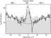Fig. B.1 CH4 (J = 6 − 5) spectrum toward Jupiter’s center from upGreat (black line) and HIFI (gray-shaded). The velocity scale refers to the Jovian system barycenter. The continuous lines refer to the synthetic spectra (with and without pressure-shift, in orange, respectively green). The dark-blue line profile is for a sightline bounded by the tropopause (p = 145 mbar in this model) and does not show the stratospheric contribution.

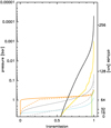Fig. B.2 As Fig. 6 but for the J = 6 − 5 line of CH4, on a sightline originating at the sub-observer point. The transmissions for this line (black) and for the broad-band opacity of CH4 (yellow) are based on the enhanced-abundance retrieval of Sánchez-López et al. (2022). Color assignments as in Fig. 2.

References

All Tables

All Figures

Fig. 1 Synoptic presentation of measurements of the fractional Jovian deuterium abundance, as determined from HD/H2 (bright green) and CH3D/CH4 (dark green). Values for Saturn, Uranus, and Neptune are shown for comparison. Deuterium fractions in various relevant environments are given as follows (from top to bottom): terrestial (dark-blue bar), represented by the Vienna standard mean ocean water (VSMOW, Gonfiantini et al. 1995); solar-wind derived (without and with corrections for protosolar 3He), orange-hatched area; high-z (violet bar); local ISM (gray-filled area). The latter comprises determinations by Linsky (1998) and, including interstellar dust, Linsky et al. (2006). For further references see main text.

In the text

Fig. 2 Vertical temperature (red) and abundance profiles against pressure altitude (ordinate), as used in the best-fit model. Abscissae (all in ppm, indicating mass fractions for ices, and volume-mixing ratios for gaseous species) are as follows: ammonia ice (green), water ice (bright blue), H2 and HD (dark blue, solid respectively dashed profile), He (medium blue), CH4 (yellow solid line, Sánchez-López et al. 2022), NH3 (orange, solid line), PH3 (orange, dotted line). The dashed yellow CH4-profile is the original abundance layering from Moses et al. (2005). For further references see Table 1.

In the text

Fig. 3 Pressure broadening γ (solid lines and dots, right ordinate) and shift δ (dashed lines and crosses, left ordinate) below 3 bar: HD-H2 for experimentally determined parameters (black, Sung et al. 2023, ≤ 1 bar) and calculated ones (green, Schaefer & Monchick 1992, for equilibrium ortho/para mixture). HD-He (theoretical) from Thibault et al. (2020, magenta), Schaefer & Monchick (1992, blue), and Stankiewicz et al. (2021, red).

In the text

	Fig. 4 Pressure altitude vs. ratio of pressure and thermal broadening (lower abscissa, solid line) and pressure-induced line shift (dashed gray, upper abscissa) as used in Sec. 5.1.
In the text

Fig. 5 HD (J = 1–0) spectrum toward Jupiter’s center, with best-fit models overlaid. The velocity scale refers to the Jovian system baryceter. Top: HD (J = 1–0) (black line and gray-filled histogram) and modeled Voigt profiles with pressure shift (red) and without (blue, the dashed profile is for a $-4_{.}^{\mathrm{\prime }\mathrm{\prime }}2$ pointing offset). Residuals and their normalized χ2 values (in brackets for the offset pointing) are shown atop (in corresponding colors, with ordinate shifts for clarity). Note the less-suppressed bandpass ripples located on the wings of the absorption profile, as discussed in section 3. Bottom: as above, but comparing the speed-dependent with the pressure-shifted Voigt profile (blue, respectively red).

In the text

Fig. 6 Profiles of the transmission in the HD, J = 1–0 line for sight-lines originating at the sub-observer point (left) and shifted along the equator to a projected distance of 0.75 Jupiter radii (${15}_{.}^{\mathrm{\prime }\mathrm{\prime }}95$), $5_{.}^{\mathrm{\prime }\mathrm{\prime }}3$ from the planet’s limb (right). The inserts show synthesized spectra for these sightlines at the same scales of (−60, +60) km s−1 and (1.4, 2.2) kJy/beam. For demonstration purposes, the spatial resolution was increased (2″ half-power width, for Nyquist-critical 1″ sampling steps) and the planet’s rotation omitted. The abscissa represents the sightline transmission $\mathcal{T}$ from a pressure altitude p0 (left ordinate, the right ordinate shows the corresponding altitude above a 6.7 bar base level) to pout toward the observer, related to the absorption coefficient κ by equation (5), with contributions from HD, J = 1–0 (black, at line center), collision-induced absorption (due to H2−H2 collisions, solid gray, and H2−He collisions, dashed gray), bright-blue (water ice), green (ammonia ice), CH4 (yellow), NH3 (orange), and PH3 (dashed orange). The color assignment is identical to that in Fig. 2. The crossings of each curve with the lower abscissa indicate the transmission from the base to the top level of the model atmospheres for the given solid or gaseous species. The area where the transmission along the sub-observer sight-line is limited by self-absorption in HD ($\mathcal{T}$self), rather than by the NH3 opacity, is highlighted in beige (left). For the off-center sightline, the gray area indicates the pressure range for which the transmission falls above $\mathcal{T}$self (right).

In the text

Fig. 7 Synthetic HD (J = 1–0) spectra. Top: five-point cross sampled at ${15}_{.}^{\mathrm{\prime }\mathrm{\prime }}95$ distance, against the gray-shaded Jupiter disk. The vertical axis coincides with the planet’s sky-plane projected rotation axis. All spectra have the same ordinate range (in K on Tmb scale) and are continuum-subtracted for clarity. The white-hatched circle centered at offset (${15}_{.}^{\mathrm{\prime }\mathrm{\prime }}95$, $0_{.}^{\mathrm{\prime }\mathrm{\prime }}0$) displays the half-power beam width of the observations. The systemic velocity is marked by vertical dotted lines. Bottom: differential spectrum between offsets ($+{15}_{.}^{\mathrm{\prime }\mathrm{\prime }}95,0_{.}^{\mathrm{\prime }\mathrm{\prime }}0$) and ($-{15}_{.}^{\mathrm{\prime }\mathrm{\prime }}95,0_{.}^{\mathrm{\prime }\mathrm{\prime }}0$) (red). The equivalent spectrum without pressure-induced line shift (gray) is shown for comparison.

In the text

Fig. A.1 Bandpass-calibration steps. Top: single-sideband calibrated spectra of Jupiter and the Moon (blue), tuned to the HD, J = 1 − 0 line and scaled in forward-beam brightness temperatures. Center: Bandpass-calibrated spectrum (normalized to unity), using the correlation shown in Fig. A.2. Bottom: After correction for atmospheric transmission and scaled to main-beam brightness temperature (Tmb, line-to-continuum ratio corrected for double-sideband reception).

In the text

	Fig. A.2 Correlation between forward-beam antenna temperatures (TA, prior to atmospheric transmission correction, on single-sideband scale) for the Moon and, at an identical spectral sampling, Jupiter.
In the text

Fig. B.1 CH4 (J = 6 − 5) spectrum toward Jupiter’s center from upGreat (black line) and HIFI (gray-shaded). The velocity scale refers to the Jovian system barycenter. The continuous lines refer to the synthetic spectra (with and without pressure-shift, in orange, respectively green). The dark-blue line profile is for a sightline bounded by the tropopause (p = 145 mbar in this model) and does not show the stratospheric contribution.

In the text

	Fig. B.2 As Fig. 6 but for the J = 6 − 5 line of CH4, on a sightline originating at the sub-observer point. The transmissions for this line (black) and for the broad-band opacity of CH4 (yellow) are based on the enhanced-abundance retrieval of Sánchez-López et al. (2022). Color assignments as in Fig. 2.
In the text

References

- Abel, M., Frommhold, L., Li, X., & Hunt, K. L. C. 2011, J. Phys. Chem. A, 115, 6805 [NASA ADS] [CrossRef] [Google Scholar]
- Abel, M., Frommhold, L., Li, X., & Hunt, K. L. C. 2012, J. Chem. Phys., 136, 044319 [NASA ADS] [CrossRef] [Google Scholar]
- Anderson, C. M., Biver, N., Bjoraker, G. L., et al. 2022, Space Sci. Rev., 218, 43 [NASA ADS] [CrossRef] [Google Scholar]
- Anguiano-Arteaga, A., Pérez-Hoyos, S., Sánchez-Lavega, A., Sanz-Requena, J. F., & Irwin, P. G. J. 2021, J. Geophys. Res. (Planets), 126, e06996 [NASA ADS] [Google Scholar]
- Appleby, J. F. 1990, Icarus, 85, 355 [NASA ADS] [CrossRef] [Google Scholar]
- Arcones, A., & Thielemann, F.-K. 2023, A&A Rev., 31, 1 [NASA ADS] [CrossRef] [Google Scholar]
- Beer, R., & Taylor, F. W. 1973, ApJ, 179, 309 [NASA ADS] [CrossRef] [Google Scholar]
- Beer, R., Farmer, C. B., Norton, R. H., Martonchik, J. V., & Barnes, T. G. 1972, Science, 175, 1360 [CrossRef] [Google Scholar]
- Bjoraker, G. L., Larson, H. P., & Kunde, V. G. 1986, Icarus, 66, 579 [NASA ADS] [CrossRef] [Google Scholar]
- Bjoraker, G. L., Wong, M. H., de Pater, I., Hewagama, T., & Ádámkovics, M. 2022, Remote Sensing, 14, 4567 [NASA ADS] [CrossRef] [Google Scholar]
- Blain, D., Fouchet, T., Greathouse, T., et al. 2018, Icarus, 314, 106 [NASA ADS] [CrossRef] [Google Scholar]
- Brown, L. R., Benner, D. C., Champion, J. P., et al. 2003, J. Quant. Spec. Radiat. Transf., 82, 219 [CrossRef] [Google Scholar]
- Cavalié, T., Benmahi, B., Hue, V., et al. 2021, A&A, 647, L8 [EDP Sciences] [Google Scholar]
- Cavalié, T., Rezac, L., Moreno, R., et al. 2023, Nat. Astron., 7, 1048 [CrossRef] [Google Scholar]
- Clayton, D. D. 1985, ApJ, 290, 428 [NASA ADS] [CrossRef] [Google Scholar]
- Combes, M., & Encrenaz, T. 1979, Icarus, 39, 1 [NASA ADS] [CrossRef] [Google Scholar]
- Combes, M., Encrenaz, T., & Owen, T. 1978, ApJ, 221, 378 [NASA ADS] [CrossRef] [Google Scholar]
- Cooke, R. J., Pettini, M., & Steidel, C. C. 2018, ApJ, 855, 102 [Google Scholar]
- Cordiner, M. A., Villanueva, G. L., Wiesemeyer, H., et al. 2022, Geophys. Res. Lett., 49, e2022GL101055 [NASA ADS] [CrossRef] [Google Scholar]
- Cordiner, M. A., Wiesemeyer, H., Villanueva, G. L., et al. 2023, Geophys. Res. Lett., 50, e2023GL106136 [NASA ADS] [CrossRef] [Google Scholar]
- Cosentino, R. G., Morales-Juberías, R., Greathouse, T., et al. 2017, J. Geophys. Res. (Planets), 122, 2719 [NASA ADS] [CrossRef] [Google Scholar]
- de Pater, I., Sault, R. J., Wong, M. H., et al. 2019, Icarus, 322, 168 [Google Scholar]
- Desch, S. J., Dunlap, D. R., Dunham, E. T., Williams, C. D., & Mane, P. 2023, Icarus, 402, 115607 [NASA ADS] [CrossRef] [Google Scholar]
- Dicke, R. H. 1953, Phys. Rev., 89, 472 [NASA ADS] [CrossRef] [Google Scholar]
- Dicke, R. H., Peebles, P. J. E., Roll, P. G., & Wilkinson, D. T. 1965, ApJ, 142, 414 [NASA ADS] [CrossRef] [Google Scholar]
- Drouin, B. J., Yu, S., Pearson, J. C., & Gupta, H. 2011, J. Mol. Struct., 1006, 2 [NASA ADS] [CrossRef] [Google Scholar]
- Duran, C. A., Gusten, R., Risacher, C., et al. 2021, IEEE Trans. Terahertz Sci. Technol., 11, 194 [CrossRef] [Google Scholar]
- Encrenaz, T. 2005, Space Sci. Rev., 116, 99 [NASA ADS] [CrossRef] [Google Scholar]
- Encrenaz, T., & Combes, M. 1982, Icarus, 52, 54 [NASA ADS] [CrossRef] [Google Scholar]
- Encrenaz, T., de Graauw, T., Schaeidt, S., et al. 1996, A&A, 315, L397 [NASA ADS] [Google Scholar]
- Es-sebbar, E.-t., & Farooq, A. 2021, J. Quant. Spec. Radiat. Transf., 272, 107758 [Google Scholar]
- Fegley, B., & Prinn, R. G. 1988, ApJ, 326, 490 [NASA ADS] [CrossRef] [Google Scholar]
- Feuchtgruber, H., Lellouch, E., Orton, G., et al. 2013, A&A, 551, A126 [NASA ADS] [CrossRef] [EDP Sciences] [Google Scholar]
- Fields, B. D., Olive, K. A., Yeh, T.-H., & Young, C. 2020, J. Cosmology Astropart. Phys., 2020, 010 [CrossRef] [Google Scholar]
- Fletcher, L. N., Orton, G. S., Sinclair, J. A., et al. 2017, Geophys. Res. Lett., 44, 7140 [NASA ADS] [CrossRef] [Google Scholar]
- Flower, D. R., & Roueff, E. 1999, MNRAS, 309, 833 [NASA ADS] [CrossRef] [Google Scholar]
- Friedman, S. D., Chayer, P., Jenkins, E. B., et al. 2023, ApJ, 946, 34 [NASA ADS] [CrossRef] [Google Scholar]
- Gamache, R. R., Roller, C., Lopes, E., et al. 2017, J. Quant. Spec. Radiat. Transf., 203, 70 [CrossRef] [Google Scholar]
- Gapp, C., Rengel, M., Hartogh, P., et al. 2024, A&A, 688, A10 [NASA ADS] [CrossRef] [EDP Sciences] [Google Scholar]
- Gautier, D., & Morel, P. 1997, A&A, 323, L9 [NASA ADS] [Google Scholar]
- Geiss, J., & Reeves, H. 1972, A&A, 18, 126 [NASA ADS] [Google Scholar]
- Geiss, J., & Gloeckler, G. 1998, Space Sci. Rev., 84, 239 [Google Scholar]
- Giles, R. S., Fletcher, L. N., & Irwin, P. G. J. 2015, Icarus, 257, 457 [NASA ADS] [CrossRef] [Google Scholar]
- Giles, R. S., Greathouse, T. K., Cosentino, R. G., Orton, G. S., & Lacy, J. H. 2020, Icarus, 350, 113905 [Google Scholar]
- Gladstone, G. R., Allen, M., & Yung, Y. L. 1996, Icarus, 119, 1 [NASA ADS] [CrossRef] [Google Scholar]
- Glover, S. C. O., & Abel, T. 2008, MNRAS, 388, 1627 [NASA ADS] [CrossRef] [Google Scholar]
- Gonfiantini, R., Stichler, W., & Rozanski, K. 1995, in Reference and Intercomparison Materials for Stable Isotopes of Light Elements, TECDOC Series No. 825 (Vienna: International Atomic Energy Agency), 13 [Google Scholar]
- Griffin, M. J., Naylor, D. A., Davis, G. R., et al. 1996, A&A, 315, L389 [NASA ADS] [Google Scholar]
- Guan, X., Stutzki, J., Graf, U. U., et al. 2012, A&A, 542, L4 [NASA ADS] [CrossRef] [EDP Sciences] [Google Scholar]
- Hartogh, P., Lellouch, E., Crovisier, J., et al. 2009, Planet. Space Sci., 57, 1596 [NASA ADS] [CrossRef] [Google Scholar]
- Hartogh, P., Lis, D. C., Bockelée-Morvan, D., et al. 2011, Nature, 478, 218 [Google Scholar]
- Hoyle, F., & Tayler, R. J. 1964, Nature, 203, 1108 [CrossRef] [Google Scholar]
- Humlícek, J. 1982, J. Quant. Spec. Radiat. Transf., 27, 437 [NASA ADS] [CrossRef] [Google Scholar]
- Kazakov, K. V. 2023, Phys. Rev. A, 108, 012801 [NASA ADS] [CrossRef] [Google Scholar]
- Kester, D., Higgins, R., & Teyssier, D. 2017, A&A, 599, A115 [NASA ADS] [CrossRef] [EDP Sciences] [Google Scholar]
- Klein, B., Hochgürtel, S., Krämer, I., et al. 2012, A&A, 542, A3 [Google Scholar]
- Kunde, V., Hanel, R., Maguire, W., et al. 1982, ApJ, 263, 443 [NASA ADS] [CrossRef] [Google Scholar]
- Lamouroux, J., Tran, H., Laraia, A. L., et al. 2010, J. Quant. Spec. Radiat. Transf., 111, 2321 [Google Scholar]
- Lecluse, C., Robert, F., Gautier, D., & Guiraud, M. 1996, Planet. Space Sci., 44, 1579 [NASA ADS] [CrossRef] [Google Scholar]
- Lellouch, E., Bézard, B., Fouchet, T., et al. 2001, A&A, 370, 610 [CrossRef] [EDP Sciences] [Google Scholar]
- Lellouch, E., Moreno, R., Orton, G. S., et al. 2015, A&A, 579, A121 [NASA ADS] [CrossRef] [EDP Sciences] [Google Scholar]
- Linsky, J. L. 1998, Space Sci. Rev., 84, 285 [NASA ADS] [CrossRef] [Google Scholar]
- Linsky, J. L., Draine, B. T., Moos, H. W., et al. 2006, ApJ, 647, 1106 [Google Scholar]
- Lis, D. C., Bockelée-Morvan, D., Güsten, R., et al. 2019, A&A, 625, L5 [NASA ADS] [CrossRef] [EDP Sciences] [Google Scholar]
- López-Puertas, M., Montañés-Rodríguez, P., Pallé, E., et al. 2018, AJ, 156, 169 [Google Scholar]
- Mahaffy, P. R., Donahue, T. M., Atreya, S. K., Owen, T. C., & Niemann, H. B. 1998, Space Sci. Rev., 84, 251 [NASA ADS] [CrossRef] [Google Scholar]
- Martonchik, J. V., Orton, G. S., & Appleby, J. F. 1984, Appl. Opt., 23, 541 [NASA ADS] [CrossRef] [Google Scholar]
- McKellar, A. R. W., Goetz, W., & Ramsay, D. A. 1976, ApJ, 207, 663 [NASA ADS] [CrossRef] [Google Scholar]
- Mielke, S. L., Peterson, K. A., Schwenke, D. W., et al. 2003, Phys. Rev. Lett., 91, 063201 [NASA ADS] [CrossRef] [Google Scholar]
- Moses, J. I., Fouchet, T., Bézard, B., et al. 2005, J. Geophys. Res. (Planets), 110, E08001 [NASA ADS] [Google Scholar]
- Mousis, O., Ronnet, T., & Lunine, J. I. 2019, ApJ, 875, 9 [NASA ADS] [CrossRef] [Google Scholar]
- Ngo, N. H., Lisak, D., Tran, H., & Hartmann, J. M. 2013, J. Quant. Spec. Radiat. Transf., 129, 89 [Google Scholar]
- Niemann, H. B., Atreya, S. K., Carignan, G. R., et al. 1996, Science, 272, 846 [CrossRef] [Google Scholar]
- Niemann, H. B., Atreya, S. K., Carignan, G. R., et al. 1998, J. Geophys. Res., 103, 22831 [NASA ADS] [CrossRef] [Google Scholar]
- Nixon, C. A., Achterberg, R. K., Conrath, B. J., et al. 2007, Icarus, 188, 47 [NASA ADS] [CrossRef] [Google Scholar]
- Orton, G. S., Appleby, J. F., & Martonchik, J. V. 1982, Icarus, 52, 94 [NASA ADS] [CrossRef] [Google Scholar]
- Orton, G. S., Gustafsson, M., Burgdorf, M., & Meadows, V. 2007, Icarus, 189, 544 [Google Scholar]
- Paine, S. 2022, am: Microwave through submillimeter-wave propagation tool for the terrestrial atmosphere, Astrophysics Source Code Library [record ascl:2205.002] [Google Scholar]
- Penzias, A. A., & Wilson, R. W. 1965, ApJ, 142, 419 [CrossRef] [Google Scholar]
- Pierel, J. D. R., Nixon, C. A., Lellouch, E., et al. 2017, AJ, 154, 178 [NASA ADS] [CrossRef] [Google Scholar]
- Planck Collaboration VI. 2020, A&A, 641, A6 [NASA ADS] [CrossRef] [EDP Sciences] [Google Scholar]
- Prodanović, T., & Fields, B. D. 2003, ApJ, 597, 48 [CrossRef] [Google Scholar]
- Pütz, P., Honingh, C. E., Jacobs, K., et al. 2012, A&A, 542, A2 [Google Scholar]
- Reeves, H., & Bottinga, Y. 1972, Nature, 238, 326 [NASA ADS] [CrossRef] [Google Scholar]
- Richard, C., Boudon, V., Manceron, L., et al. 2023, Icarus, 404, 115692 [NASA ADS] [CrossRef] [Google Scholar]
- Richter, M. J., Dewitt, C. N., McKelvey, M., et al. 2018, J. Astron. Instrum., 7, 1840013 [NASA ADS] [CrossRef] [Google Scholar]
- Riemer-Sørensen, S., Kotuš, S., Webb, J. K., et al. 2017, MNRAS, 468, 3239 [CrossRef] [Google Scholar]
- Risacher, C., Güsten, R., Stutzki, J., et al. 2018, J. Astron. Instrum., 7, 1840014 [NASA ADS] [CrossRef] [Google Scholar]
- Rohatgi, A. 2022, Webplotdigitizer: Version 4.6, https://automeris.io/WebPlotDigitizer [Google Scholar]
- Rood, R. T., Steigman, G., & Tinsley, B. M. 1976, ApJ, 207, L57 [NASA ADS] [CrossRef] [Google Scholar]
- Rood, R. T., Bania, T. M., & Wilson, T. L. 1992, Nature, 355, 618 [NASA ADS] [CrossRef] [Google Scholar]
- Roueff, E., Abgrall, H., Czachorowski, P., et al. 2019, A&A, 630, A58 [NASA ADS] [CrossRef] [EDP Sciences] [Google Scholar]
- Sánchez-López, A., López-Puertas, M., García-Comas, M., et al. 2022, A&A, 662, A91 [NASA ADS] [CrossRef] [EDP Sciences] [Google Scholar]
- Schaefer, J., & Monchick, L. 1992, A&A, 265, 859 [NASA ADS] [Google Scholar]
- Simon-Miller, A. A., Conrath, B., Gierasch, P. J., & Beebe, R. F. 2000, Icarus, 145, 454 [NASA ADS] [CrossRef] [Google Scholar]
- Smith, W. H., Schempp, W. V., & Baines, K. H. 1989, ApJ, 336, 967 [NASA ADS] [CrossRef] [Google Scholar]
- Stankiewicz, K., Stolarczyk, N., Jóźwiak, H., Thibault, F., & Wcisło, P. 2021, J. Quant. Spec. Radiat. Transf., 276, 107911 [CrossRef] [Google Scholar]
- Sung, K., Devi, V. M., Benner, D. C., et al. 2020, J. Quant. Spec. Radiat. Transf., 256, 107264 [CrossRef] [Google Scholar]
- Sung, K., Wishnow, E. H., Drouin, B. J., et al. 2023, J. Quant. Spec. Radiat. Transf., 295, 108412 [CrossRef] [Google Scholar]
- Thibault, F., Martínez, R. Z., Bermejo, D., & Wcisło, P. 2020, Mol. Astrophys., 19, 100063 [NASA ADS] [CrossRef] [Google Scholar]
- Tran, H., Flaud, P. M., Fouchet, T., Gabard, T., & Hartmann, J. M. 2006, J. Quant. Spec. Radiat. Transf., 101, 306 [NASA ADS] [CrossRef] [Google Scholar]
- Tran, H., Ngo, N. H., & Hartmann, J. M. 2013, J. Quant. Spec. Radiat. Transf., 129, 199 [CrossRef] [Google Scholar]
- Trauger, J. T., Roesler, F. L., Carleton, N. P., & Traub, W. A. 1973, ApJ, 184, L137 [CrossRef] [Google Scholar]
- Tsujimoto, T. 2011, MNRAS, 410, 2540 [NASA ADS] [CrossRef] [Google Scholar]
- Tyler, R. H. 2022, Planet. Sci. J., 3, 250 [NASA ADS] [CrossRef] [Google Scholar]
- Vasavada, A. R., Bandfield, J. L., Greenhagen, B. T., et al. 2012, J. Geophys. Res. (Planets), 117, E00H18 [CrossRef] [Google Scholar]
- Villanueva, G. L., Smith, M. D., Protopapa, S., Faggi, S., & Mandell, A. M. 2018, J. Quant. Spec. Radiat. Transf., 217, 86 [NASA ADS] [CrossRef] [Google Scholar]
- von Zahn, U., Hunten, D. M., & Lehmacher, G. 1998, J. Geophys. Res., 103, 22815 [NASA ADS] [CrossRef] [Google Scholar]
- Warren, S. G. 1984, Appl. Opt., 23, 1206 [NASA ADS] [CrossRef] [Google Scholar]
- West, R. A. 2014, in Encyclopedia of the Solar System, 3rd edn., eds. T. Spohn, D. Breuer, & T. V. Johnson (Boston: Elsevier), 723 [CrossRef] [Google Scholar]
- Wiesemeyer, H., Güsten, R., Aladro, R., et al. 2023, Phys. Rev. Res., 5, 013072 [NASA ADS] [CrossRef] [Google Scholar]
- Williams, J. P., Paige, D. A., Greenhagen, B. T., & Sefton-Nash, E. 2017, Icarus, 283, 300 [CrossRef] [Google Scholar]
- Wishnow, E. H., Orton, G. S., Ozier, I., & Gush, H. P. 2007, J. Quant. Spec. Radiat. Transf., 103, 102 [CrossRef] [Google Scholar]
- Yurchenko, S. N., Owens, A., Kefala, K., & Tennyson, J. 2024, MNRAS, 528, 3719 [CrossRef] [Google Scholar]
- Zhang, X., West, R. A., Irwin, P. G. J., Nixon, C. A., & Yung, Y. L. 2015, Nat. Commun., 6, 10231 [NASA ADS] [CrossRef] [Google Scholar]
- Zuchowski, L. C., Yamazaki, Y. H., & Read, P. L. 2009, Icarus, 200, 563 [NASA ADS] [CrossRef] [Google Scholar]
JPL Horizons on-line Solar System data and ephemeris computation service, https://ssd.jpl.nasa.gov/horizons/
All Tables
Spectroscopic parameters used in the radiative transfer of the CH (J = 6 − 5) multiplet.