| Issue |
A&A
Volume 688, August 2024
|
|
|---|---|---|
| Article Number | A68 | |
| Number of page(s) | 13 | |
| Section | Stellar atmospheres | |
| DOI | https://doi.org/10.1051/0004-6361/202449873 | |
| Published online | 06 August 2024 | |
The enigma of Li-rich giants and its relation with temporal variations observed in radial velocity and stellar activity signals
1
Instituto de Astrofísica e Ciências do Espaço, Universidade do Porto, CAUP,
Rua das Estrelas,
4150-762
Porto,
Portugal
e-mail: This email address is being protected from spambots. You need JavaScript enabled to view it.
2
Departamento de Física e Astronomia, Faculdade de Ciências, Universidade do Porto,
Rua do Campo Alegre 687,
4169-007
Porto,
Portugal
3
INAF – Osservatorio Astrofisico di Arcetri,
Largo E. Fermi 5,
50125
Firenze,
Italy
Received:
6
March
2024
Accepted:
22
June
2024
Abstract
Context. Despite the large number of studies focused on the characterisation of Li-rich stars and understanding the mechanisms leading to such enrichment, their origin remains a mystery.
Aims. Magnetic activity, particularly the phenomena usually associated with it (e.g. spots and plages), and the Li abundance (A(Li)) of stars, are in general thought to be connected. As of today, however, just how they are connected is unclear. In this work, we study a sample of young but evolved intermediate-mass red giants that are inhabitants of open clusters where planets have been searched for. Our aim is to use radial velocity (RV) and stellar activity indicator signals to look for relations between Li abundances and stellar activity or variability.
Methods. We explored how the standard deviation (STD), peak-to-peak amplitude (PTP), mean, and median of typical stellar activity indicators (BIS, FWHM, Teff, and Hα index) change as a function of the Li content of 82 red giants. Furthermore, we computed weighted Pearson correlation coefficients (ρw) between time series of RV measurements and the stellar activity indicators for the stars in our sample. To aid our results, we also studied generalized Lomb–Scargle periodograms (GLSP) to capture possible significant periodic temporal variations in our data.
Results. Our analysis indicates that the STD and PTP of BIS and FWHM, the mean and median of the Hα index, and υ sin(i) increase exponentially with A(Li) in our sample of red giants. Significant temporal variations and correlations between RVs and activity indicators also tend to be found preferentially for stars where high A(Li) is observed. Most of the Li-rich stars in our sample either show strong correlations of RV with at least one of the stellar activity indicators or reveal significant periodic temporal variations in their GLSPs of stellar activity indicators that are consistent with those found for RV.
Key words: stars: abundances / stars: activity / planetary systems / stars: rotation / stars: statistics
© The Authors 2024
 Open Access article, published by EDP Sciences, under the terms of the Creative Commons Attribution License (https://creativecommons.org/licenses/by/4.0), which permits unrestricted use, distribution, and reproduction in any medium, provided the original work is properly cited.
This article is published in open access under the Subscribe to Open model. This email address is being protected from spambots. You need JavaScript enabled to view it. to support open access publication.
1 Introduction
Before entering the red giant branch (RGB) of their evolution, low- (≲2 M⊙) to intermediate-mass stars (~2–8 M⊙) (Iben 1967a,b) go through a mixing episode called the first dredge up (FDU), which destroys most, if not all, of their surface lithium (Li). Stars as massive as the Sun, according to standard stellar evolution models, should not exhibit a surface lithium abundance, A (Li)1, exceeding 1.5 dex after the FDU. In general, observations concur with this, but ~1% of observed giants (e.g. Brown et al. 1989; Kumar et al. 2011; Liu et al. 2014; Casey et al. 2016; Kirby et al. 2016; Deepak & Reddy 2019; Gao et al. 2019; Pabst et al. 2020; Martell et al. 2021) present abnormally high A(Li), with the highest abundance observed to date in a red giant star being 5.62 dex (Kowkabany et al. 2022). These stars are known as Li-rich giants.
Possible explanations for the Li enrichment observed in these stars fall under two main categories. First, it has been proposed that a star may show high levels of surface Li if it has been contaminated by an external source. For example, if planet engulfment occurs, the Li content of the planet can be laid out in the photosphere of the star and enrich it (e.g. Adamów et al. 2012; Aguilera-Gómez et al. 2016; Delgado Mena et al. 2016). On the other hand, under certain conditions, Li can be synthe-sised inside a star and rise to the surface through extra mixing processes. For stars with mass >4 M⊙ in the asymptotic giant branch (AGB) of their evolution, the Cameron-Fowler mechanism (CFM; (Cameron & Fowler 1971)) is the preferred scenario to explain Li enrichment. In these stars, the temperature at the bottom of the convective envelope is favourable to the production of beryllium, which when transported fast enough to the outer layers of the star can produce Li without it being destroyed. In lower-mass stars, high enough temperatures for beryllium production can only be found inwards of the convective envelope. For these stars, the existence of extra mixing mechanisms such as thermohaline mixing (e.g. Eggleton et al. 2008; Cantiello & Langer 2010) and rotation-induced mixing (e.g. Denissenkov & Herwig 2004; Palacios et al. 2006; Adamów et al. 2014) are more plausible, as they are needed to bring the beryllium from the deeper layers to the convective envelope so that CFM can ensue. One way to probe extra mixing scenarios is by analysing the surface carbon isotopic ratio 12C/13C, which after the FDU occurs is lowered to values of about 20–30 (Charbonnel 1994; Denissenkov & Herwig 2004). Further lowering of 12C/13C is a good and widely used indication that extra mixing occurred in a star (Charbonnel 1995; Aguilera-Gómez et al. 2023; Lagarde et al. 2024).
It is also generally accepted that higher than normal A(Li) is common among magnetically active stars, even if the reason for this is still poorly understood. This has been shown in different types of stars, including dwarfs (Favata et al. 1996; Zboril et al. 1997); magnetically peculiar stars (see Lyubimkov 2016 for a review); active binaries and pre-main-sequence stars (Pallavicini et al. 1992); active main-sequence and zero-age main-sequence stars (Xing et al. 2021); and active giant stars (Fekel & Balachandran 1994; Sneden et al. 2022).
In this work, we are interested in studying the possible connection between Li enhancement in red giant stars and their stellar activity. As such, we started by looking for relations between several descriptive statistics of stellar activity indicators and A(Li) in a sample of red giant stars, some of which are lithium rich, where planets have been searched. These stars are inhabitants of open clusters, which is particularly favourable, as we are able to better constrain their evolutionary status. To strengthen our analysis, we also looked for correlations as well as periodic temporal variations in stellar activity signals that may connect the variability observed in radial velocity (RV) to stellar activity. The present article is organised as follows: In Sect. 2, we provide an overview of our data. In Sect. 3, we explain the methods incurred in the data analysis. In Sect. 4, we discuss our results, and the main conclusions are laid out in Sect. 5.
2 Observations and sample
Our sample is composed of young but evolved intermediate-mass red giants residing in ten different open clusters (IC4651, IC4756, NGC2345, NGC2423, NGC3114, NGC3532, NGC3680, NGC4349, NGC5822, and NGC6705). These stars have been observed over the years with the HARPS spectrograph (Mayor et al. 2003) at the ESO 3.6-m telescope (R = 115 000) and the CORALIE spectrograph (Queloz et al. 2000; Udry et al. 2000) at the Swiss 1.2-metre Leonhard Euler Telescope at ESO’s La Silla Observatory (R = 60 000) as part of a programme to search for exoplanets. (For a complete description of the RV surveys see Lovis & Mayor 2007; Delgado Mena et al. 2018; Delgado Mena et al. 2023.) The stellar parameters and Li abundances for this sample are presented in Tsantaki et al. (2023), who used the same spectra employed here.
In this work, the data available from CORALIE are not treated. CORALIE data carry a much higher associated uncertainty in the measurements than HARPS data due to a significantly lower resolution (R). Furthermore, CORALIE data were only collected for a subset of stars in our sample, and the measurements for each star are few in number. For these reasons we preferred to use only HARPS data.
Only stars with five or more observational data points were considered for analysis. This limitation increases the credibility of our results while including the most observed stars as possible. In total, 82 stars were analysed out of which 15 are canonically Li rich, that is they show A(Li)>1.5 dex. If a Population I star forming with a metallicity similar to that of the Sun has in the beginning of its life A(Li)~3.3 dex, that is, the approximate A(Li) of the interstellar medium, accounting for the dilution occurring during the FDU, it should be left with a maximum of A(Li)~1.5 dex in the red giant phase of its evolution (e.g. Char-bonnel & Balachandran 2000). Studying stars in open clusters, however, allows for a more precise estimate of this limit. Open clusters are ideal laboratories for studying Li enhancement given that they provide natural constraints on the mass, composition, age, and evolutionary state of their members. With such information, it is possible to estimate the amount of Li that all stars in a given cluster should have at their current age using stellar evolution models. This allows us to better constrain what makes a star in a given cluster ‘Li rich’ (see Sun et al. 2022). Tsantaki et al. (2023) conducted such a study, providing estimations for the maximum A(Li) that stars in 32 different open clusters should have in their current evolutionary stage. Stars are considered Li rich according to the limits defined in Table 1 and the canonical definition. Special attention is given to stars that show high Li content in comparison to inhabitants of the same cluster in the same evolutionary stage. We deem such stars ‘Li-Rich-in-Context’, in accordance with Tsantaki et al. (2023) and Sun et al. (2022). All relevant stars are presented in Table 2. Some of these stars have been studied previously in the literature. A thorough discussion concerning the possible nature of the Li enrichment observed in these stars has been provided in Tsantaki et al. (2023), and it is summarised in Table 2.
Limits over which a star can be considered lithium rich for every cluster in our sample (A(Li)max (dex)).
3 Methods
To probe if the high A(Li) that we observe in red giant stars is connected to their stellar activity, we explored two methods. First, we studied how Li abundances relate to the following stellar activity indicators:
- 1.
the bisector inverse slope (BIS) of the cross correlation function;
- 2.
the full width at half maximum (FWHM) of the cross correlation function;
- 3.
the Hα index with both a 0.6 Å and 1.6 Å central bandpass (Hα06, Hα16);
- 4.
and the effective temperature (Teff).
In particular, we looked for relations between A(Li) and the standard deviation (STD) and peak-to-peak amplitude (PTP) of all stellar activity indicators as well as the mean and median of Hα. Only statistically significant models at a 99% confidence level (with p-values of the F-test <0.0l) are discussed.
Secondly, we investigated if a possible connection between A(Li) and stellar activity manifests in RV variability. So, we sought correlations between stellar activity indicators and RV measurements (see Fig. C.1). These were computed according to the Pearson correlation coefficient, ρw, which is weighted here by the uncertainty in the measurements. The p-values for each correlation are also provided to attest to the statistical significance of the correlations. A p-value bellow 0.05 suggests that the correlation is significantly different from zero at a 95% confidence level. In addition, periodic temporal variations of the RV measurements of these stars and the stellar activity indicators were analysed by drawing generalised Lomb-Scargle Periodograms (GLSPs (Zechmeister & Kürster 2009)) in order to evaluate if they connect to the presence of Li.
When searching for planets, it is important to devise methods to distinguish planetary signals from temporal variability that may arise from the phenomena appearing at the surface of a star as a consequence of stellar magnetic activity. The BIS and FWHM values of each observation are provided by the HARPS data reduction pipeline as part of the process to calculate the RV of a given spectrum. Correlations found between RV and respective BIS and FWHM measurements indicate that periodical variability noticed in RV signals may originate from stellar activity or stellar surface inhomogeneities rather than planets. Variability observed in BIS and FWHM over time with approximately the same period as that observed in RV can also further corroborate this. These types of studies have often been conducted to probe whether or not a planet really exists in the orbit of a certain star (e.g. Queloz et al. 2001; Delgado Mena et al. 2018).
In studying how stellar activity impacts an RV signal, it is common to analyse spectral lines that serve as an activity proxy due to their well-known correlations with the existence of active regions on the surface of a star. One such spectral line is the Hα line. Here, we determined Hα index values from spectra using ACTIN 22 (Gomes da Silva et al. 2018, 2021). This tool to calculate stellar activity indices provides two measurements for the Hα index for two different central bandpasses: 0.6 Å and 1.6 Å (see Fig. C.2). Since it has been mostly used for dwarf stars (Gomes da Silva et al. 2022), there is a lack of an extensive study for stars such as the ones in our sample, and it is not clear which central bandpass is optimal for the study of these stars. Recently, in analysing the strong RV signals of some of the stars in this sample (Delgado Mena et al. 2023), we found that Hα16 seems to be a more reliable activity indicator for these evolved stars. But this conclusion was based on a small sample. As such, and since the two bandpasses probe the stellar atmosphere at different layers that are sensitive to different phenomena, we used both bandpasses in our analysis.
We further extended our search for correlations and periodical variations to the Teff. Manifestations of magnetic activity, much like spots and plages are usually accompanied by temperature variations. Spots are cooler than their surrounding photosphere, while plages are hotter than their surrounding chromosphere. During periods of intense magnetic activity, it is possible that if the Teff is affected, the variations observed could correlate with the activity-induced variations (e.g. Yana Galarza et al. 2019). We used the stellar spectral analysis package FASMA3 (Tsantaki et al. 2018) to determine the Teff from individual stellar spectra. FASMA relies on the radiative transfer code MOOG4 (Sneden 1973) to model the atmosphere and create a synthetic spectrum for a set of input parameters of a given star, which include surface gravity, log(g); iron metallicity, [Fe/H]; macro-turbulence velocity υmac; and projected rotational velocity υ sin(i). The synthetic spectrum was then statistically compared to the observed spectrum of the star, and the parameters were iteratively adjusted using a non-linear least-squares algorithm in order to find the set that best fits the observations. To capture reliable variations in Teff, when computing it, we fixed all other input stellar parameters and left Teff to be computed freely for each individual stellar spectra. Stellar parameters for the stars in our sample have been derived in Tsantaki et al. (2023) also by using FASMA.
Lithium-rich and ‘Li-Rich-in-Context’ giants present in our sample.
4 Results and discussion
As presented in Table 2 and in accordance with Mermilliod et al. (2008), the star NGC3532No649 is not a member of cluster NGC3532, making the calculation of its mass and evolutionary stage uncertain. For this reason, it is not included in the following discussion despite it being Li rich.
4.1 The relationship between lithium abundance and stellar activity in red giants
We started by analysing the dispersion (STD and PTP) of BIS, FWHM, Teff, and Hα in order to probe for any potential connections between activity variability and A(Li). We also tested if the mean and median of Hα, which are indicative of a star’s activity level, are related to A(Li). For the computation of these relations, we only used stars with A(Li)> –0.5, as this is the limit of FASMA’s minimisation algorithm in the determination of A(Li) (Tsantaki et al. 2023). Using these limit values would be a source of bias. We find that the STD and PTP of BIS and FWHM increase exponentially with A(Li), and the mean and median values of Hα06 also increase exponentially with A(Li). In particular, the vast majority of stars with a high Hα06 index are Li enriched. On the other hand, we did not find A(Li) to be related to Hα16. These results suggest that the activity levels of the stars in our sample seem to increase with increasing A(Li). These results are in agreement with Sneden et al. (2022), who found that Li-rich giants are more chromospherically active in comparison to their Li-poor counterparts, as they are more likely to show strong He Iλ10830 absorptions. We also find that υ sin(i) correlates well with the dispersion of BIS and FHWM as well as the mean and median of the Hα06 index. This is indicative that more magnetically active stars also tend to rotate faster. Gonçalves et al. (2020) also arrived at a similar conclusion. The best-fit relations are listed in Table 3. Plots of the relations found for the STD of BIS and FWHM as well as the mean of Hα06 are shown in Fig. 1. The plots for the PTP of BIS and FWHM and the median of Hα06 look similar to the ones shown in Fig. 1 and are presented in Appendix D. Also in Appendix D are plots of the mean and median Hα16 as a function of A(Li), for which no clear relation was found. In addition to the results of the F-test, in Table 3 we also provide R2 values, with better fits having R2 closer to one. The R2 values for the relations we found are in general low, as there is significant scatter around the lines of the best fit.
Best-fit relations of the descriptive statistics of the stellar activity indicators and υ sin(i) as a function of A(Li).
4.2 Manifestation of stellar activity in radial velocity signals and its connection to lithium enhancement
To further investigate these findings, we also looked at how RV variability correlates with the stellar activity indicators and whether this is linked to A(Li). All the correlations discussed here are shown in Fig. 2 and listed in Appendix B. From our analysis, 22/81 stars show a strong correlation (>0.45) between the RV variability and the BIS variability. The majority of the correlations were found to be negative. As stars age, their υ sin(i) decreases, typically falling below 5 km s–1 by the end of the main-sequence (e.g. de Medeiros et al. 1996; Tayar et al. 2015; Patton et al. 2024). We noticed that 13/22 of the strong correlations found between RV and BIS appear for stars that are moderate and fast rotators (υsin(i) > 5 km s−1). This is likely a consequence of this diagnostic of line asymmetry losing sensitivity for slower rotators (e.g. Santos et al. 2003). There is, however, evidence in the literature (e.g. Carlberg et al. 2012; Sneden et al. 2022; Sayeed et al. 2024; Tsantaki et al. 2023) that there is a connection between Li enrichment in giants and υ sin(i). This is also suggested in our sample, as we find that υ sin(i) increases exponentially with A(Li) (shown in Appendix D and Table 3). Out of the 27 Li-rich stars listed in Table 2, eight stars show strong correlations between RV and BIS.
In what concerns the FWHM, 20/81 stars show strong correlations with RV measurements. The correlations are preferentially positive. Six of the Li-rich stars in our sample show strong correlations between RV and FWHM.
For the Teff, we find that 15/81 stars show strong correlations with RV measurements. Correlations between the RV and Teff are mostly positive. Only three of the Li-rich stars show strong correlations between RV and Teff. There is a possibility that this the case is because the individual spectra used to measure Teff values to look for variations may not have a signal-to-noise ratio high enough for this purpose.
As for Hαl6, 20/81 stars show strong correlations with RV, and they are mostly negative. Nine of the Li-rich stars show strong correlations between RV and Hαl6.
Last but not least, for Hα06, 19/81 stars show significant correlations with RV measurements, and they are preferentially positive. We find that ten of the Li-rich stars in our sample show strong correlations between RV and Hα06.
Overall, correlations were found for stars in various evolutionary stages and of different mass ranges as well. This is evidenced in the Hertzsprung–Russell (HR) diagram in Fig. 3, where different symbols indicate different numbers of strong correlations found per star and the data points are sized according to stellar mass. In general, all symbols display a range of sizes and are distributed across the HR diagram, revealing there is no preferred mass or age for correlations to be found. A summary of the significant correlations discussed can be found in Tables A.1 and A.2. Something to note from Table A.2 is that inhabitants of cluster NGC6705, in general, show higher amounts of Li than the rest of the stars in our sample. These stars are particular, as they also demonstrate unusually high amounts of α-elements for their young age (e.g. Casamiquela et al. 2018). Messina et al. (2010) found that the G-type stars of this cluster retain higher levels of activity up to the age of the cluster. We find that 19/28 of these stars show at least one significant correlation with one of the parameters we studied, and 22/28 are fast rotators (see Table A.2). So, in general, the stars in this cluster are magnetically active and also rotate fast, which could be connected to the abnormally high levels of Li observed.
In Fig. 4, we show a violin plot of A(Li) as a function of the number of strong correlations observed per star. One may see that the density of the points increases towards higher values of A(Li), with an increasing number of correlations found. This is evidenced by the increasing width of the violins from left to right in high A(Li) regions and by the central tendency being slightly higher for stars that show one or more than two correlations between RV and stellar activity indicators. As such, strong correlations tend to appear more often for stars with higher amounts of Li in their atmospheres. Such a result also indicates that A(Li) seems to be connected with higher levels of stellar activity in our sample.
To complement the correlation analysis, GLSPs of RV and stellar activity indicators were also plotted for all stars. The GLSPs are often used when analysing whether variability observed in RV signals is caused by the existence of a companion or by stellar activity. This is because they make it possible to determine if there is periodic variability occurring at the stellar surface that is equivalent to the periodic variability observed in RV. It has been shown that magnetic phenomena appearing at the stellar surface can introduce variability in RV that is at a different phase relative to the variability observed in stellar activity indicator signals (e.g. Queloz et al. 2001; Santos et al. 2014; Delgado Mena et al. 2018). As such, when looking for correlations between RV and activity proxies, we may obtain a weak correlation coefficient, but this does not necessarily mean that the RV variability does not originate from stellar activity. Thus, finding peaks at similar periods in RV and again in different stellar activity signals with GLSP is also an indicator that RV variability connects with stellar activity.
The results of the GLSP analysis are also presented in Tables A.1 and A.2. In summary, stars NGC2345No50, NGC2423No3, NGC3532No670, NGC4349Nol27, and NGC670No110 show significant peaks (above a false-alarm probability (FAP) level of 1%) in their RV GLSPs, which consistently appear around the same period for at least one of their stellar activity indicators. All relevant GLSPs are in Appendix E and Delgado Mena et al. (2023). All of these stars can be considered Li rich (see Table 2), and most of them also present long-term and large amplitude RV variations that mimic the presence of planets but are of probable stellar origin (Delgado Mena et al. 2023). These stars with periodic RV variations lie on the RGB or RGB tip (they are among the most luminous in their cluster) rather than in the red clump, as found in recent works for super-Li-rich stars (Singh et al. 2019; Kumar et al. 2020). Interestingly, Jorissen et al. (2020), studying the binarity fraction of Li-rich giants, found that some of the most luminous Li-rich giants show RV variability not caused by stellar companions, though no information about stellar activity is provided by the authors. Similarly, Gonçalves et al. (2020) found hints of RV variability in several Li-rich stars with a detected longitudinal magnetic field, but the quantity of data does not permit one to discern the real origin of such variability.
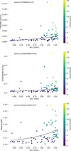 |
Fig. 1 Exponential relation found between the STD of BIS data for each star and A(Li) [top panel], the STD of FWHM data for each star and A(Li) [middle panel], and the mean of Hα06 data for each star and A(Li) [bottom panel]. The data points are coloured according to the υ sin(i) of each star. The black lines are the lines of best fit for which the F-test statistics and p-values are listed in Table 3. In these plots we also show the Pearson correlation coefficients (p) between the activity proxies used and υ sin(i); all of them are very strong (>0.6). |
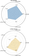 |
Fig. 2 Spider charts showing the number of strong correlations found. The top chart shows how many strong correlations were found between RV and every stellar activity indicator in the full sample of red giant stars. The bottom chart shows how many strong correlations were found between RV and every stellar activity indicator for the stars of interest listed in Table 2. |
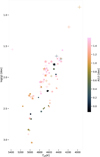 |
Fig. 3 Hertzsprung-Russell diagram of all the stars in our sample. Here we use the log(g) and Teff derived in Tsantaki et al. (2023) for each star. The stars are coloured according to A(Li) and have different sizes to represent their different masses. The different symbols indicate how many strong correlations were found in a particular star: “•” indicates zero strong correlations, “★” indicates one strong correlation, and “+” indicates two or more strong correlations. |
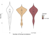 |
Fig. 4 Violin plot of A(Li) as a function of the number of strong correlations observed per star. From left to right, each violin represents the distribution of the number of strong correlations found (0, 1, or ≥ 2) relative to A(Li). Inside each violin is a box delimiting the interquartile range. The thick black line appearing inside each box is the median of the distribution. Each box also has a lower and upper whisker that spans from minimum to maximum A(Li) in each distribution. Points seen beyond the whiskers are outliers. |
5 Conclusions
In summary, based on the results from the HARPS data, we find that the variability of BIS and FWHM and the mean and median of Hα06 increase exponentially with A(Li). This leads us to conclude that the stars in our sample that are more magnetically active also show higher amounts of Li in their atmosphere. We also find that stars with higher amounts of Li tend to show more correlations between RV and stellar activity indicators. The majority of the stars, 19/27 (10/14 leaving aside the special cluster NGC6705), that can be considered Li rich in this work either show correlations of RV with at least one of the stellar activity indicators or show periodic variability in at least one of the stellar activity indicator signals with a similar period in RV. From the GLSP analysis we may also conclude that almost all the stars with strong RV variations that mimic the presence of planets are Li rich (see also, Delgado Mena et al. 2016). This is particularly important when searching for exoplanets orbiting evolved stars since our results show that detecting periodic RV variability in red giants with high A(Li) might be a signature of stellar activity instead of planets. It is interesting to note that Adamów et al. (2018) reported a higher than expected fraction of planetary companions around the Li-rich stars in their sample, pointing to a connection between Li enrichment and planetary presence or engulfment. However, the orbits they found are quite eccentric, something not expected if the RV is of stellar origin, and that characteristic supports the hypothesis of inner planet engulf-ment. The Li-rich stars with strong RV variability discussed here lie on the RGB or RGB tip. However, stars showing correlations between Li abundance and activity level are found all across the HR diagram. This might indicate that mild Li enrichment (since we do not have super Li-rich giants in our sample) connected to stellar activity can occur at different evolutionary stages, but a large enhancement of Li is more particular and can only occur at certain evolutionary stages, such as the He flash stage (Singh et al. 2019; Kumar et al. 2020). Thus, it is still not clear whether the strong RV variability of mild Li-rich giants on the RGB is connected to their evolutionary stage and the possible super Li-rich phase that happens soon after (at the beginning of the He-core burning phase) or if it is a consequence of stellar activity.
Acknowledgements
We thank the anonymous referee for the insightful comments and suggestions. I.R. and E.D.M. acknowledge the support from Fun-dação para a Ciência e a Tecnologia (FCT) through national funds and from FEDER through COMPETE2020 by the following grants: UIDB/04434/2020 & UIDP/04434/2020. I.R. acknowledges the support from FCT through the grant 2022.03993.PTDC. E.D.M. acknowledges the support from FCT through Stimulus FCT contract 2021.01294.CEECIND. E.D.M. and J.G.S. acknowledge the support from FCT through the grant 2022.04416.PTDC. This work made use of scientific colour maps (https://www.fabiocrameri.ch/colourmaps/; Crameri et al. 2020) to mitigate visual distortion.
Appendix A Additional tables
Summary of strong correlations found for the stars analysed in clusters IC4651, IC4756, NGC2345, NGC2423, NGC3114, NGC3532, NGC3680, NGC4349 and NGC5822.
Summary of strong correlations found for the stars analysed in cluster NGC6705.
Appendix B Correlation tables
Correlations found for all of the stars in our sample.
Appendix C Methods for data analysis
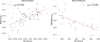 |
Fig. C.1 Example of strong correlations found for stars NGC2423No3 (left) and NGC2345No50 (right). NGC2423No3 shows a strong positive correlation between RV and BIS, while NGC23545No50 shows a strong negative correlation between RV and FWHM. |
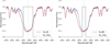 |
Fig. C.2 Example of the Hα line profile difference of two spectra obtained at different times for star NGC2345No50 (depicted by the blue and red lines). In black are represented the two different bandpasses (Hα16 on the left and Hα06 on the right), around the Hα line centre, used to compute the Hα index for the individual spectra of the stars with ACTIN 2. |
Appendix D Additional relations
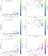 |
Fig. D.1 Left: Exponential relation found between the PTP of BIS data for each star and A(Li) [top panel]; the PTP of FWHM data for each star and A(Li) [middle panel]; the median of Hα06 data for each star and A(Li) [bottom panel]. The data points are coloured according to the υ sin(i) of each star. The black line is the line of best fit. In these plots we also show the Pearson Correlation Coefficients (ρ) between the activity proxies used and υ sin(i), all of them being very strong (> 0.6). Right: No relation found between the mean and median of Hα16 data for each star and A(Li) [top and middle panels, respectively]. Here again the data points are coloured according to the υ sin(i) of each star and ρ between the activity proxies and υ sin(i) is also shown, being weak in both cases. In the bottom panel we show the exponential relation found between υ sin(i) and A(Li). The data points are coloured according to the strength of the correlations of ρw(BIS) to demonstrate that the majority of correlations found for this indicator appear for moderate and fast rotators (υ sin(i) >5 km/s). The black line is the line of best fit. |
Appendix E Generalized Lomb-Scargle periodograms
The remainder of the GLPs mentioned in the text can be found in Delgado Mena et al. (2023).
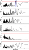 |
Fig. E.1 Generalised Lomb-Scargle periodograms pertaining to star NGC6705No1101 for BIS, FWHM, Teff, and Hα. The red line indicates a false alarm probability level of 1%. Significant peaks are observed in the RV and BIS GLSPs at approximately the same period. There is also a significant peak observed in FWHM not related to those observed in RV. |
References
- Adamów, M., Niedzielski, A., Villaver, E., Nowak, G., & Wolszczan, A. 2012, ApJ, 754, L15 [Google Scholar]
- Adamów, M., Niedzielski, A., Villaver, E., Wolszczan, A., & Nowak, G. 2014, A&A, 569, A55 [NASA ADS] [CrossRef] [EDP Sciences] [Google Scholar]
- Adamów, M., Niedzielski, A., Kowalik, K., et al. 2018, A&A, 613, A47 [NASA ADS] [CrossRef] [EDP Sciences] [Google Scholar]
- Aguilera-Gómez, C., Chanamé, J., Pinsonneault, M. H., & Carlberg, J. K. 2016, ApJ, 829, 127 [Google Scholar]
- Aguilera-Gómez, C., Jones, M. I., & Chanamé, J. 2023, A&A, 670, A73 [NASA ADS] [CrossRef] [EDP Sciences] [Google Scholar]
- Bagdonas, V., Drazdauskas, A., Tautvaišiene, G., Smiljanic, R., & Chorniy, Y. 2018, A&A, 615, A165 [NASA ADS] [CrossRef] [EDP Sciences] [Google Scholar]
- Brown, J. A., Sneden, C., Lambert, D. L., & Dutchover, Edward, J. 1989, ApJS, 71, 293 [NASA ADS] [CrossRef] [Google Scholar]
- Cameron, A. G. W., & Fowler, W. A. 1971, ApJ, 164, 111 [NASA ADS] [CrossRef] [Google Scholar]
- Cantiello, M., & Langer, N. 2010, A&A, 521, A9 [NASA ADS] [CrossRef] [EDP Sciences] [Google Scholar]
- Carlberg, J. K., Cunha, K., Smith, V. V., & Majewski, S. R. 2012, ApJ, 757, 109 [NASA ADS] [CrossRef] [Google Scholar]
- Casamiquela, L., Carrera, R., Balaguer-Núñez, L., et al. 2018, A&A, 610, A66 [NASA ADS] [CrossRef] [EDP Sciences] [Google Scholar]
- Casey, A. R., Ruchti, G., Masseron, T., et al. 2016, MNRAS, 461, 3336 [NASA ADS] [CrossRef] [Google Scholar]
- Charbonnel, C. 1994, A&A, 282, 811 [NASA ADS] [Google Scholar]
- Charbonnel, C. 1995, ApJ, 453, L41 [NASA ADS] [CrossRef] [Google Scholar]
- Charbonnel, C., & Balachandran, S. C. 2000, A&A, 359, 563 [Google Scholar]
- Crameri, F., Shephard, G. E., & Heron, P. J. 2020, Nat. Commun., 11, 5444 [NASA ADS] [CrossRef] [Google Scholar]
- de Medeiros, J. R., Melo, C. H. F., & Mayor, M. 1996, A&A, 309, 465 [NASA ADS] [Google Scholar]
- Deepak, & Reddy, B. E. 2019, MNRAS, 484, 2000 [NASA ADS] [Google Scholar]
- Delgado Mena, E., Tsantaki, M., Sousa, S. G., et al. 2016, A&A, 587, A66 [NASA ADS] [CrossRef] [EDP Sciences] [Google Scholar]
- Delgado Mena, E., Lovis, C., Santos, N. C., et al. 2018, A&A, 619, A2 [NASA ADS] [CrossRef] [EDP Sciences] [Google Scholar]
- Delgado Mena, E., Gomes da Silva, J., Faria, J. P., et al. 2023, A&A, 679, A94 [NASA ADS] [CrossRef] [EDP Sciences] [Google Scholar]
- Denissenkov, P. A., & Herwig, F. 2004, ApJ, 612, 1081 [NASA ADS] [CrossRef] [Google Scholar]
- Eggleton, P. P., Dearborn, D. S. P., & Lattanzio, J. C. 2008, ApJ, 677, 581 [NASA ADS] [CrossRef] [Google Scholar]
- Favata, F., Micela, G., & Sciortino, S. 1996, A&A, 311, 951 [NASA ADS] [Google Scholar]
- Fekel, F. C., & Balachandran, S. 1994, in Cool Stars, Stellar Systems, and the Sun, 64, 279 [NASA ADS] [Google Scholar]
- Frinchaboy, P. M., & Majewski, S. R. 2008, AJ, 136, 118 [NASA ADS] [CrossRef] [Google Scholar]
- Gao, Q., Shi, J.-R., Yan, H.-L., et al. 2019, ApJS, 245, 33 [NASA ADS] [CrossRef] [Google Scholar]
- Gomes da Silva, J., Figueira, P., Santos, N., & Faria, J. 2018, J. Open Source Softw., 3, 667 [Google Scholar]
- Gomes da Silva, J., Santos, N. C., Adibekyan, V., et al. 2021, A&A, 646, A77 [NASA ADS] [CrossRef] [EDP Sciences] [Google Scholar]
- Gomes da Silva, J., Bensabat, A., Monteiro, T., & Santos, N. C. 2022, A&A, 668, A174 [NASA ADS] [CrossRef] [EDP Sciences] [Google Scholar]
- Gonçalves, B. F. O., da Costa, J. S., de Almeida, L., Castro, M., & do Nascimento, J. D., J. 2020, MNRAS, 498, 2295 [CrossRef] [Google Scholar]
- Herzog, A. D., Sanders, W. L., & Seggewiss, W. 1975, A&AS, 19, 211 [NASA ADS] [Google Scholar]
- Holanda, N., Pereira, C. B., & Drake, N. A. 2019, MNRAS, 482, 5275 [NASA ADS] [CrossRef] [Google Scholar]
- Holanda, N., Ramos, A. A., Peña Suárez, V. J., Martinez, C. F., & Pereira, C. B. 2022, MNRAS, 516, 4484 [NASA ADS] [CrossRef] [Google Scholar]
- Iben, Icko, J. 1967a, ApJ, 147, 650 [NASA ADS] [CrossRef] [Google Scholar]
- Iben, Icko, J. 1967b, ApJ, 147, 624 [NASA ADS] [CrossRef] [Google Scholar]
- Jorissen, A., Van Winckel, H., Siess, L., et al. 2020, A&A, 639, A7 [NASA ADS] [CrossRef] [EDP Sciences] [Google Scholar]
- Katime Santrich, O. J., Pereira, C. B., & Drake, N. A. 2013, A&A, 554, A2 [NASA ADS] [CrossRef] [EDP Sciences] [Google Scholar]
- Kirby, E. N., Guhathakurta, P., Zhang, A. J., et al. 2016, ApJ, 819, 135 [NASA ADS] [CrossRef] [Google Scholar]
- Kowkabany, J., Ezzeddine, R., Charbonnel, C., et al. 2022, arXiv e-prints [arXiv:2209.02184] [Google Scholar]
- Kumar, Y. B., Reddy, B. E., & Lambert, D. L. 2011, ApJ, 730, L12 [NASA ADS] [CrossRef] [Google Scholar]
- Kumar, Y. B., Reddy, B. E., Campbell, S. W., et al. 2020, Nat. Astron., 4, 1059 [NASA ADS] [CrossRef] [Google Scholar]
- Lagarde, N., Minkeviciute, R., Drazdauskas, A., et al. 2024, A&A, 684, A70 [NASA ADS] [CrossRef] [EDP Sciences] [Google Scholar]
- Liu, Y. J., Tan, K. F., Wang, L., et al. 2014, ApJ, 785, 94 [NASA ADS] [CrossRef] [Google Scholar]
- Lovis, C., & Mayor, M. 2007, A&A, 472, 657 [NASA ADS] [CrossRef] [EDP Sciences] [Google Scholar]
- Luck, R. E. 1994, ApJS, 91, 309 [NASA ADS] [CrossRef] [Google Scholar]
- Lyubimkov, L. S. 2016, Astrophysics, 59, 411 [NASA ADS] [CrossRef] [Google Scholar]
- Martell, S. L., Simpson, J. D., Balasubramaniam, A. G., et al. 2021, MNRAS, 505, 5340 [NASA ADS] [Google Scholar]
- Mayor, M., Pepe, F., Queloz, D., et al. 2003, The Messenger, 114, 20 [NASA ADS] [Google Scholar]
- Mermilliod, J. C., Mayor, M., & Udry, S. 2008, A&A, 485, 303 [NASA ADS] [CrossRef] [EDP Sciences] [Google Scholar]
- Messina, S., Parihar, P., Koo, J.-R., et al. 2010, A&A, 513, A29 [NASA ADS] [CrossRef] [EDP Sciences] [Google Scholar]
- Pabst, C. H. M., Goicoechea, J. R., Teyssier, D., et al. 2020, A&A, 639, A2 [NASA ADS] [CrossRef] [EDP Sciences] [Google Scholar]
- Palacios, A., Charbonnel, C., Talon, S., & Siess, L. 2006, in Chemical Abundances and Mixing in Stars in the Milky Way and its Satellites, eds. S. Randich, & L. Pasquini (Berlin, Heidelberg: Springer Berlin Heidelberg), 304 [Google Scholar]
- Pallavicini, R., Randich, S., & Giampapa, M. S. 1992, A&A, 253, 185 [NASA ADS] [Google Scholar]
- Patton, R. A., Pinsonneault, M. H., Cao, L., et al. 2024, MNRAS, 528, 3232 [NASA ADS] [CrossRef] [Google Scholar]
- Peña Suárez, V. J., Sales Silva, J. V., Katime Santrich, O. J., Drake, N. A., & Pereira, C. B. 2018, ApJ, 854, 184 [CrossRef] [Google Scholar]
- Queloz, D., Mayor, M., Weber, L., et al. 2000, A&A, 354, 99 [NASA ADS] [Google Scholar]
- Queloz, D., Henry, G. W., Sivan, J. P., et al. 2001, A&A, 379, 279 [NASA ADS] [CrossRef] [EDP Sciences] [Google Scholar]
- Randich, S., Pasquini, L., Franciosini, E., et al. 2020, A&A, 640, L1 [EDP Sciences] [Google Scholar]
- Romano, D., Magrini, L., Randich, S., et al. 2021, A&A, 653, A72 [NASA ADS] [CrossRef] [EDP Sciences] [Google Scholar]
- Santos, N. C., Udry, S., Mayor, M., et al. 2003, A&A, 406, 373 [NASA ADS] [CrossRef] [EDP Sciences] [Google Scholar]
- Santos, N. C., Mortier, A., Faria, J. P., et al. 2014, A&A, 566, A35 [NASA ADS] [CrossRef] [EDP Sciences] [Google Scholar]
- Sayeed, M., Ness, M. K., Montet, B. T., et al. 2024, ApJ, 964, 42 [NASA ADS] [CrossRef] [Google Scholar]
- Singh, R., Reddy, B. E., Bharat Kumar, Y., & Antia, H. M. 2019, ApJ, 878, L21 [NASA ADS] [CrossRef] [Google Scholar]
- Smiljanic, R., Gauderon, R., North, P., et al. 2009, A&A, 502, 267 [NASA ADS] [CrossRef] [EDP Sciences] [Google Scholar]
- Sneden, C. A. 1973, PhD thesis, The University of Texas at Austin, USA [Google Scholar]
- Sneden, C., Af¸ar, M., Bozkurt, Z., et al. 2022, ApJ, 940, 12 [NASA ADS] [CrossRef] [Google Scholar]
- Sun, Q., Deliyannis, C. P., Twarog, B. A., et al. 2022, MNRAS, 513, 5387 [NASA ADS] [CrossRef] [Google Scholar]
- Tayar, J., Ceillier, T., García-Hernández, D. A., et al. 2015, ApJ, 807, 82 [NASA ADS] [CrossRef] [Google Scholar]
- Tsantaki, M., Andreasen, D. T., Teixeira, G. D. C., et al. 2018, MNRAS, 473, 5066 [NASA ADS] [CrossRef] [Google Scholar]
- Tsantaki, M., Delgado-Mena, E., Bossini, D., et al. 2023, A&A, 674, A157 [NASA ADS] [CrossRef] [EDP Sciences] [Google Scholar]
- Udry, S., Mayor, M., Naef, D., et al. 2000, A&A, 356, 590 [NASA ADS] [Google Scholar]
- Xing, L.-F., Li, Y.-C., Chang, L., Wang, C.-J., & Bai, J.-M. 2021, A&A, 653, A28 [NASA ADS] [CrossRef] [EDP Sciences] [Google Scholar]
- Yana Galarza, J., Meléndez, J., Lorenzo-Oliveira, D., et al. 2019, MNRAS, 490, L86 [Google Scholar]
- Zboril, M., Byrne, P. B., & Rolleston, W. R. J. R. 1997, MNRAS, 284, 685 [NASA ADS] [CrossRef] [Google Scholar]
- Zechmeister, M., & Kürster, M. 2009, A&A, 496, 577 [CrossRef] [EDP Sciences] [Google Scholar]
A(Li) = log[N(Li)/N(H)] + 12.
Some of the analysed stars in our sample do not have a large number of data points. Because of this, we chose to include moderate correlations that have the potential to become strong with the addition of new data. For ease of nomenclature, we refer to all correlations greater than 0.4 as strong.
All Tables
Limits over which a star can be considered lithium rich for every cluster in our sample (A(Li)max (dex)).
Best-fit relations of the descriptive statistics of the stellar activity indicators and υ sin(i) as a function of A(Li).
Summary of strong correlations found for the stars analysed in clusters IC4651, IC4756, NGC2345, NGC2423, NGC3114, NGC3532, NGC3680, NGC4349 and NGC5822.
Summary of strong correlations found for the stars analysed in cluster NGC6705.
All Figures
|
Fig. 1 Exponential relation found between the STD of BIS data for each star and A(Li) [top panel], the STD of FWHM data for each star and A(Li) [middle panel], and the mean of Hα06 data for each star and A(Li) [bottom panel]. The data points are coloured according to the υ sin(i) of each star. The black lines are the lines of best fit for which the F-test statistics and p-values are listed in Table 3. In these plots we also show the Pearson correlation coefficients (p) between the activity proxies used and υ sin(i); all of them are very strong (>0.6). |
| In the text | |
|
Fig. 2 Spider charts showing the number of strong correlations found. The top chart shows how many strong correlations were found between RV and every stellar activity indicator in the full sample of red giant stars. The bottom chart shows how many strong correlations were found between RV and every stellar activity indicator for the stars of interest listed in Table 2. |
| In the text | |
|
Fig. 3 Hertzsprung-Russell diagram of all the stars in our sample. Here we use the log(g) and Teff derived in Tsantaki et al. (2023) for each star. The stars are coloured according to A(Li) and have different sizes to represent their different masses. The different symbols indicate how many strong correlations were found in a particular star: “•” indicates zero strong correlations, “★” indicates one strong correlation, and “+” indicates two or more strong correlations. |
| In the text | |
|
Fig. 4 Violin plot of A(Li) as a function of the number of strong correlations observed per star. From left to right, each violin represents the distribution of the number of strong correlations found (0, 1, or ≥ 2) relative to A(Li). Inside each violin is a box delimiting the interquartile range. The thick black line appearing inside each box is the median of the distribution. Each box also has a lower and upper whisker that spans from minimum to maximum A(Li) in each distribution. Points seen beyond the whiskers are outliers. |
| In the text | |
|
Fig. C.1 Example of strong correlations found for stars NGC2423No3 (left) and NGC2345No50 (right). NGC2423No3 shows a strong positive correlation between RV and BIS, while NGC23545No50 shows a strong negative correlation between RV and FWHM. |
| In the text | |
|
Fig. C.2 Example of the Hα line profile difference of two spectra obtained at different times for star NGC2345No50 (depicted by the blue and red lines). In black are represented the two different bandpasses (Hα16 on the left and Hα06 on the right), around the Hα line centre, used to compute the Hα index for the individual spectra of the stars with ACTIN 2. |
| In the text | |
|
Fig. D.1 Left: Exponential relation found between the PTP of BIS data for each star and A(Li) [top panel]; the PTP of FWHM data for each star and A(Li) [middle panel]; the median of Hα06 data for each star and A(Li) [bottom panel]. The data points are coloured according to the υ sin(i) of each star. The black line is the line of best fit. In these plots we also show the Pearson Correlation Coefficients (ρ) between the activity proxies used and υ sin(i), all of them being very strong (> 0.6). Right: No relation found between the mean and median of Hα16 data for each star and A(Li) [top and middle panels, respectively]. Here again the data points are coloured according to the υ sin(i) of each star and ρ between the activity proxies and υ sin(i) is also shown, being weak in both cases. In the bottom panel we show the exponential relation found between υ sin(i) and A(Li). The data points are coloured according to the strength of the correlations of ρw(BIS) to demonstrate that the majority of correlations found for this indicator appear for moderate and fast rotators (υ sin(i) >5 km/s). The black line is the line of best fit. |
| In the text | |
|
Fig. E.1 Generalised Lomb-Scargle periodograms pertaining to star NGC6705No1101 for BIS, FWHM, Teff, and Hα. The red line indicates a false alarm probability level of 1%. Significant peaks are observed in the RV and BIS GLSPs at approximately the same period. There is also a significant peak observed in FWHM not related to those observed in RV. |
| In the text | |
Current usage metrics show cumulative count of Article Views (full-text article views including HTML views, PDF and ePub downloads, according to the available data) and Abstracts Views on Vision4Press platform.
Data correspond to usage on the plateform after 2015. The current usage metrics is available 48-96 hours after online publication and is updated daily on week days.
Initial download of the metrics may take a while.