| Issue |
A&A
Volume 697, May 2025
|
|
|---|---|---|
| Article Number | A32 | |
| Number of page(s) | 28 | |
| Section | Planets, planetary systems, and small bodies | |
| DOI | https://doi.org/10.1051/0004-6361/202453500 | |
| Published online | 05 May 2025 | |
Precise radial velocities of giant stars
XVII. Distinguishing planets from intrinsically induced radial velocity signals in evolved stars
1
Landessternwarte, Zentrum für Astronomie der Universität Heidelberg,
Königstuhl 12,
69117
Heidelberg,
Germany
2
Department of Astronomy, Faculty of Physics, Sofia University “St Kliment Ohridski”,
5 James Bourchier Blvd,
1164
Sofia,
Bulgaria
3
Stellar Astrophysics Centre, Department of Physics and Astronomy, Aarhus University,
Ny Munkegade 120,
8000
Aarhus C,
Denmark
4
Instituto de Astrofísica de Canarias,
38200
La Laguna, Tenerife,
Spain
5
Universidad de La Laguna (ULL), Departamento de Astrofísica,
38206
La Laguna, Tenerife,
Spain
★ Corresponding author: dane.spaeth@lsw.uni-heidelberg.de
Received:
18
December
2024
Accepted:
11
March
2025
Context. From a long-term Doppler monitoring campaign of 373 giant stars, we have identified ten giants with periodic radial velocity variations that are challenging to associate with planets. Similar cases in the literature are attributed to poorly understood intrinsic processes.
Aims. Our goal is to confirm or refute the presence of planets around these ten evolved stars. Additionally, we evaluate the reliability and sensitivity of planet-confirmation metrics when applied to giant stars and present cases of intrinsically induced radial velocity variations, aiming to enhance the physical understanding of the phenomenon.
Methods. We combined 25 years of radial velocity data from the Hamilton/Lick, SONG, and CARMENES spectrographs. To assess consistency with Keplerian models, we examined the residuals and tracked changes in statistical significance as new data were incorporated. Additionally, we compared radial velocity amplitudes across optical and infrared wavelengths, searched for periodic variations of activity indicators, and examined their correlations with radial velocities.
Results. Seven of the ten giants exhibit intrinsically induced radial velocity variations. The strongest arguments against planets orbiting the giants are guided by long-term radial velocity monitoring that detects changing periodicity on long timescales or detects systematics close to the original period in the radial velocity residuals. While activity indicators offer some support, their signals are generally weak. Comparing optical and infrared radial velocity amplitudes also proves insufficient for confirming or refuting planets. We find HIP 64823 remains a promising candidate for hosting a giant exoplanet with orbital period P ∼ 7.75 yr. For two stars, the evidence remains inconclusive.
Conclusions. Long-term radial velocity monitoring is essential for distinguishing planetary companions from intrinsic variations in evolved stars.
Key words: techniques: radial velocities / planets and satellites: detection / stars: evolution / stars: oscillations / planetary systems
© The Authors 2025
 Open Access article, published by EDP Sciences, under the terms of the Creative Commons Attribution License (https://creativecommons.org/licenses/by/4.0), which permits unrestricted use, distribution, and reproduction in any medium, provided the original work is properly cited.
This article is published in open access under the Subscribe to Open model. Subscribe to A&A to support open access publication.
1 Introduction
The majority of the over 5750 exoplanets confirmed to date have been detected via the transit technique (∼ 75%) and the radial velocity (RV) method (∼ 19%)1. Each of the exoplanet detection methods, however, has intrinsic biases that leave a large part of the exoplanet parameter space still to be explored.
For instance, main-sequence stars more massive than about 1.5 M⊙ are challenging to target in both transit (due to the larger radii) and RV surveys. For the latter, the achievable RV precision is limited due to high surface temperatures resulting in a small number of absorption lines, which are significantly broadened by high rotation rates (Sato et al. 2003; Galland et al. 2005; Johnson et al. 2007; Lagrange et al. 2009; Assef et al. 2009). An alternative to studying the population of planets around these stars is to target their evolved counterparts, which have significantly cooled down and slowed their rotation velocities, resulting in numerous narrow absorption lines that contain valuable Doppler information. So far, around 150 planets orbiting giant stars have been detected2, the vast majority of which were found using the RV method.
A recent study by Wolthoff et al. (2022) summarizes the planet occurrence rate around giant stars through a combined analysis of three large RV surveys. They show a positive planet-metallicity correlation, as previously found also for main-sequence stars (Fischer & Valenti 2005; Udry & Santos 2007) and for giants (Reffert et al. 2015). Furthermore, Wolthoff et al. (2022) report a peak in the planet-occurrence rate at host masses M = 1.68 ± 0.59 M⊙ and at orbital periods of around 2 yr.
However, the RV method applied to giant stars faces two important challenges. On the one hand, short-term p-mode (solar-like) oscillations lead to intrinsic RV jitter with amplitudes around 10 to 20 m s−1, even for relatively stable giant stars (Hekker et al. 2006). The amplitude of these p-mode oscillations increases as the stars become more evolved and luminous (Hekker et al. 2008), and thus the oscillations present more of a challenge for such giants. However, as the periods of these oscillations are typically on scales of hours to days, they can be dealt with as a white noise component in the context of exoplanet surveys targeting companions with orbital periods of several hundred days. Nevertheless, while this short-term RV jitter complicates the detection of low-mass (M ≲ 1 MJup) planetary companions, the detection of planets of higher masses is not impacted.
On the other hand, what is more problematic is the suspicion that the RV signals of some of the most luminous evolved planet hosts are in fact caused by poorly understood intrinsic stellar processes instead of planetary companions. The first identified case was γ Dra (Hatzes et al. 2018), which showed stable large-amplitude RV variations with a period of P ∼ 700 d during nearly eight years of RV monitoring before amplitude changes and phase shifts became apparent. Other stars with RV signals with similar periods have been found in subsequent studies and include Aldebaran (Reichert et al. 2019), ϵ Cyg (Heeren et al. 2021), 42 Dra (Döllinger & Hartmann 2021), Sanders 3643 (Zhou et al. 2023), HD 135438 (Lee et al. 2023), and four evolved stars in open clusters: NGC 2423 No. 3, NGC 2345 No. 50, NGC 3532 No. 670, and NGC 4349 No. 1274 (Delgado Mena et al. 2018, 2023). For several of the stars, the RV variations had previously been attributed to planetary companions. We stress that all of these stars are very luminous (L > 100 L⊙) and that false-positive detections seem to occur frequently only for stars with radii R ≳ 21 R⊙ and RV periods between 300 d and 800 d (Döllinger & Hartmann 2021). Planets around less luminous giants are generally not contested.
The arguments to refute orbital companions as the origin of the RV signals of these luminous giants are quite varied. The orbital companions for γ Dra, Aldebaran, ϵ Cyg, and 42 Dra have been ruled out based on arguments of the coherence and stability of the RV signal, which are only possible after extensive, long-term RV monitoring. The planet around Sanders 364 was ruled out, as periodicity at multiple periods was detected (Zhou et al. 2023). On the other hand, for the cluster giants presented by Delgado Mena et al. (2018,2023), orbital companions have been ruled out based on variations of the activity indicators identified with the High Accuracy Radial Velocity Planet Searcher (HARPS; Mayor et al. 2003). Unfortunately, such additional spectral diagnostics are mostly only available from pressure and temperature stabilized spectrographs with stable instrumental profiles. Furthermore, since not all published planets have been monitored on sufficiently long timescales or have a large set of reliable activity indicators available, there could, in principle, be more as yet unidentified false-positive planets around the most luminous giants, especially around those that have been announced on the basis of sparse RV sampling.
Furthermore, the origin of these intrinsic RV variations is still uncertain. The long RV periods typically rule out radial pulsations (Hatzes & Cochran 1993; Cox et al. 1972; Hatzes et al. 2018; Reichert et al. 2019). The modulation of magnetic surface spots is one possibility, but it would in most cases lead to a larger photometric variability than detected (Reffert et al. 2015). More exotic magnetic processes, potentially linked to convection, that could lead to RV variations without associated photometric variations have been suggested (Delgado Mena et al. 2023; Rolo et al. 2024), but they remain poorly studied. For the binary star ϵ Cyg, the heartbeat phenomenon was put forth (Heeren et al. 2021), but it cannot explain the variations for single stars. Finally, non-radial oscillations have been discussed for a long time as being a potential source of intrinsic RV variations (Hatzes & Cochran 1994; Hatzes 1996; Hatzes & Cochran 1998).
Oscillatory convective modes have been proposed as the origin of non-radial oscillations in very luminous photometrically variable giant stars (Saio et al. 2015), although it is unclear whether these would be applicable for the less luminous giants within the group of false positives. In a recent study, we have shown that simulations of an l = 1, m = 1 non-radial oscillation can reproduce the variations of the RVs and the activity indicators of NGC 4349 No. 127 (Spaeth et al. 2024), an evolved cluster giant reported to host a brown-dwarf companion (Lovis & Mayor 2007) but the finding has since been refuted by Delgado Mena et al. (2018,2023). However, it remains to be seen if other stars can be shown to have similar signatures.
The goal of this study is three-fold. (i) Our initial motivation was to investigate whether a number of so-far unpublished planet candidates identified in the Lick RV survey of giant stars are exoplanets or false-positives by intrinsic variations. These candidates were followed up using spectrographs from the Stellar Observations Network Group (SONG) and the Calar Alto high-Resolution search for M dwarfs with Exoearths with Near-infrared and optical Echelle Spectrographs (CARMENES). (ii) With nearly 25 years of RV data and a set of activity indicators commonly used to target planets orbiting main-sequence stars, we further aimed to test which metrics that determine the difference between planets and intrinsic variations are sensitive to intrinsic phenomena in evolved stars. (iii) Last, we aim to present further intrinsically RV-variable stars as well as their observational fingerprints, hoping to contribute toward a better physical understanding of the intrinsic mechanism present in giant stars that can mimic planetary companions quite convincingly in RV data. For this purpose, we present ten such planet candidates along with two secure exoplanet systems. For simplicity, we include all orbital companions of substellar minimum mass within the term “planet” unless stated otherwise.
The paper is structured as follows. In Sect. 2, we give an overview of the sample and the stellar parameters followed by a summary of the observations in Sect. 3. In Sect. 4, we discuss the RV time series data along with several metrics aimed at differentiating between planets and intrinsic processes causing the (semi-)periodic RV variations. These metrics are discussed star-by-star in Sect. 5. In Sect. 6, we explore the most promising planet candidate, HIP 64823, remaining after the activity analysis. Finally, we discuss potential astrophysical origins of the intrinsic variations in Sect. 7 and summarize our findings in Sect. 8.
2 Sample and stellar parameters
The giant stars considered in this work were originally part of the Lick RV survey, which started in 1999 and targeted 373 bright (V ≤ 6) G and K giants. The Lick sample initially comprised 86 K giants, selected to be photometrically stable and not part of multiple systems from the HIPPARCOS catalog (Frink et al. 2001; ESA 1997). The stellar sample was extended in 2000 and 2004, relaxing the constraints on photometric stability and adding stars with higher masses and bluer colors. However, the actual level of photometric variability remained below 0.01 mag for most stars (Reffert et al. 2015).
Stellar parameters derived by Stock et al. (2018).
Overall, 18 planets in 15 stellar systems present in the Lick sample of giant stars have been confirmed either by our own or other groups (Frink et al. 2002; Hatzes et al. 2006; Reffert et al. 2006; Sato et al. 2007; Liu et al. 2008; Schwab 2010; Wittenmyer et al. 2011; Mitchell et al. 2013; Trifonov et al. 2014; Lee et al. 2014; Ortiz et al. 2016; Takarada et al. 2018; Quirrenbach et al. 2019; Luque et al. 2019; Tala Pinto et al. 2020; Hill et al. 2021; Teng et al. 2023a). A recent overview is also presented by Wolthoff et al. (2022). Furthermore, a number of stars were identified as periodic RV-variable stars, making them planet-host candidates. 20 stars of the latter group, along with three confirmed planet hosts were monitored using CARMENES starting in 2017 (see Sect. 3). Notably, the 20 planet candidates also include HIP 16335, for which a planetary companion was published by Lee et al. (2014), but that we classified as a candidate. In this work, we exclude stars with long-period (much longer than the combined Lick-CARMENES baseline) stellar companions as the uncertainty of the outer companions’ orbits significantly hinders the analysis. We further exclude two stars that will be the focus of future dedicated publications. The remaining sample of 12 stars thus comprises ten giants that were considered to be candidates to host planets with periods between one and eight years after the Lick survey concluded as well as two published planet hosts, namely ι Dra (HIP 75458) (Frink et al. 2002; Hill et al. 2021) and ν Oph (HIP 88048) (Quirrenbach et al. 2011, 2019), which were added to the CARMENES observations for comparison.
The stellar parameters for the Lick giant star sample have been derived by Stock et al. (2018) using Bayesian inference on a grid of stellar evolutionary models, implemented in the fitting tool SPOG+.5 The stellar parameters in the most likely evolutionary state, either on the red giant branch (RGB) or horizontal branch (HB), are presented in Table 1. Many of the stars are relatively luminous. The stars are roughly evenly distributed between the RGB and HB (five vs seven). The solar-like oscillations of HIP 75458 and HIP 89826 have been analyzed as part of asteroseismic studies (Zechmeister et al. 2008; Hill et al. 2021; Campante et al. 2023; Malla et al. 2024). The derived asteroseismic parameters are consistent with those in Table 1.
Figure 1 shows the loci of the 12 stars, as well as the remaining 361 giants comprising the Lick sample, within a Gaia DR3 (Gaia Collaboration 2016, 2023) color-magnitude diagram. For the stars not present in the Gaia catalog due to their brightness (including HIP 46390), we converted the HIPPARCOS photometric measurements (ESA 1997) into the Gaia passbands6. To provide a visual reference, we overplot the fifth catalog of nearby stars (CNS5; Golovin et al. 2023) and three PARSEC evolutionary tracks (Bressan et al. 2012) for different stellar masses at solar metallicity.
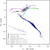 |
Fig. 1 Color-magnitude diagram based on Gaia DR3 photometry showing the location of the sample stars using blue star markers as well as red diamonds for the two published planet hosting giants ι Dra and ν Oph. We also plot the location of the remaining 361 giant stars within the Lick sample in purple. For comparison, we overplot the fifth catalog of nearby stars (CNS5) (Golovin et al. 2023) in dark blue and three adjacent evolutionary tracks for 1 M⊙ (green), 2 M⊙ (black), and 3 M⊙ (purple) taken from PARSEC (Bressan et al. 2012). |
3 Observations
3.1 Lick observations
The observations at UCO/Lick Observatory started in 1999 using the 0.6 m Coudé Auxiliary Telescope (CAT) and the Hamilton Echelle Spectrometer (Vogt 1987) with a measured resolving power R ∼ 50 000 at 6000 Å (Reffert et al. 2015). The survey used the iodine technique described by Butler et al. (1996) and aimed for an RV precision of 5 to 8 m s−1 (Reffert et al. 2015). The Hamilton spectrograph covers a wavelength range of approximately 3400–9000 Å (Fischer et al. 2013). However, the RV determination is limited to the regime spanning roughly 5000−5800 Å, due to the use of the iodine cell. The observations ended in 2011 when the iodine cell at Lick was damaged (Fischer et al. 2013). A continuation of the survey using the 72 cm Waltz Telescope located at Landessternwarte Heidelberg (Tala et al. 2016) is expected to start in 2025. Overall, 1127 Lick spectra are available for the 12 stars with a time baseline of approximately 12 years. We use the standard Lick RV reduction.
3.2 Lick Hα index
Since the line spread function of the Lick spectra is comparably unstable (Tala Pinto et al. 2020), and due to the inclusion of the iodine cell, activity indicators targeting the shape of the stellar spectral lines only yield low precision (see, for instance, Reffert et al. 2006). No such indicators are therefore used in this work.
An individual spectral line that is present in the Lick wavelength range, lies outside the iodine regime, and is known to be sensitive to chromospheric activity (Kürster et al. 2003), is the Hα line (6562.8 Å). To quantify the variability of its core, we improved upon the work by Staudt (2020), who calculates Hα indices for the Lick spectra based on the definition by Boisse et al. (2009). Since the standard wavelength regions used by Staudt (2020) and Boisse et al. (2009) were strongly affected by telluric lines, we searched for relatively unaffected regions within the spectral order containing the Hα line and slightly redefine the Hα index as
 (1)
(1)
with FHα being the flux in a 0.4 Å region centered on the core of the Hα line and F1−5 being the fluxes in five smaller comparison regions in the continuum. These are defined as [6538.5 Å, 6540.5 Å, [6565.0 Å, 6567.0 Å], [6576.0 Å, 6578.0 Å], [6582.5 Å, 6584.5 Å], and [6595.0 Å, 6597.0 Å]. The uncertainties were calculated by quadratically adding the contributions of the estimated intensity error using the βσ procedure (Stoehr et al. 2008; Czesla et al. 2018) and the influence of an imperfect wavelength shift by performing a Monte Carlo simulation (Staudt 2020). The Hα time series is treated as two separate data sets due to small offsets caused by a CCD camera exchange in April 2004 (some spectra testing the new CCD have already been acquired in 2002/2003).
3.3 SONG observations
After the Lick observations concluded, select giants from the Lick survey were monitored using the 1 m robotic SONG telescope located on Tenerife, Spain (Andersen et al. 2014; Fredslund Andersen et al. 2019). The SONG spectrograph is a high-resolution (R ∼ 90 000), cross-dispersed échelle spectrograph. Similar to the Lick survey, SONG employs the iodine cell technique to derive precise RVs (Grundahl et al. 2017). The SONG spectrograph covers the wavelength range 4400–6900 Å (Grundahl et al. 2017), with RVs derived from the regime 5000 Å to 6300 Å (Heeren et al. 2023).
Of the 12 stars in the sample, four (HIP 38253, HIP 46390, HIP 47959, and HIP 75458) were included in the SONG observations. Overall 1030 spectra with sufficient S/N are available from SONG between March 2015 and December 2023. We obtained the RVs using the pyodine reduction software (Heeren et al. 2023). No standard activity indicators are available from the SONG observations. We note that some spectra, especially for HIP 75458, were taken as part of other observing campaigns aiming to study short-term variations. In these cases, several (typically less than five, in two nights more than ten) spectra were taken in the same night. Nevertheless, we refrain from binning the spectra, as retaining the full time resolution of the measurements can help to constrain the short-term jitter during the RV modeling.
3.4 CARMENES observations
First CARMENES observations for the ten planet candidates were taken between 2017 and 2018 (with a single additional spectrum from 2016). These include archival spectra from other observation programs. The CARMENES observations were continued, after an unfortunate gap, from 2021 to 2023 for the full sample, including the confirmed planet hosts.
The CARMENES spectrograph (Quirrenbach et al. 2014), installed at the 3.5 m telescope at Calar Alto, Spain, offers two independent channels acquiring spectra in different wavelength regimes simultaneously. The visual (VIS) channel covers the regime 5200 Å to 9600 Å, with a resolving power R ∼ 94 600. The near-infrared (NIR) channel continues the coverage at longer wavelengths from 9600 Å to 17 100 Å with a resolving power R ∼ 80 4007.
We reduced the CARMENES data using two reduction pipelines. The standard SERVAL reduction pipeline (Zechmeister et al. 2018) uses a coadded stellar template to derive the RVs using least squares minimization. The pipeline furthermore yields several activity indicators, namely the chromatic index (CRX), differential linewidth (dLW) (see Zechmeister et al. 2018 for their definitions), and several line indicators: Hα (6562.8 Å), Na I D1 (5895.9 Å), Na I D2 (5889.9 Å), and the Ca II infrared triplet (IRT) lines at 8498.0 Å, 8542.1 Å, and 8662.1 Å. For brevity, we refer to the line indicators as NaDi and CaIRTi, respectively. These indicators have been shown to be sensitive to chromospheric activity (see, for instance, Kürster et al. 2003; Díaz et al. 2007; Martínez-Arnáiz et al. 2011; Martin et al. 2017; Schöfer et al. 2019; Huang et al. 2024; Gehan et al. 2024).
Due to the brightness of the stars (V ≤ 6 mag), they are excellent filler targets and have been observed in variable, sometimes even quite bad, observing conditions. As a consequence, the S/N of the individual observations varies, although it is generally high. Additionally, in some good nights exposure times were increased in an attempt to reach sufficient S/N in the simultaneous Fabry-Pérot exposures to measure the instrumental drift over the course of the night (Schäfer et al. 2018). As a consequence, a few observations have S/N exceeding the standard SERVAL limits of 500 and 400 for the visual and near-infrared channels, respectively. To avoid any non-linear effects due to a saturation of the CCD affecting all observations, we first created a SERVAL template using only spectra below the standard SERVAL S/N limits, which we then used to derive the RVs and activity indicators for all spectra. Other than that, we use the standard settings of the SERVAL pipeline for the two respective CARMENES channels. We note that this includes the selection of only a subset of the NIR spectral orders, as many orders suffer from severe telluric contamination (Reiners et al. 2018; Nagel et al. 2023).
We furthermore derived the RVs and activity indicators by calculating the cross-correlation function (CCF) with a weighted binary mask by using the RACCOON reduction software (Lafarga et al. 2020). The RACCOON pipeline yields spectral diagnostics such as the full width at half maximum (FWHM) and contrast of the CCF, as well as the bisector inverse slope (BIS). By default, masks are only provided for M dwarfs targeted in the CARMENES GTO sample (Reiners et al. 2018; Ribas et al. 2023). We therefore calculated new masks for each star using the functionality provided by RACCOON and the SERVAL templates detailed above. The RACCOON RVs are generally in good agreement with the SERVAL results. The deviation of the RV results between the SERVAL and RACCOON results have a standard deviation σ = 3.3 m s−1 and σ = 11.6 m s−1 for VIS and NIR, respectively. The larger deviations in the near infrared are expected due to a lower number of usable lines as reported by Lafarga et al. (2020). For the analysis presented in Sect. 4, we always use the RVs as derived by SERVAL, and complement these with the FWHM, contrast, and BIS measurements derived by RACCOON.
Although it was attempted to obtain instrumental drift measurements for the spectra simultaneously, exposure times were often too short to ensure sufficient Fabry-Pérot exposures in the second fiber of the CARMENES spectrograph. For these spectra, the instrumental drift was modeled over the night with a third-order polynomial using the drift measurements from the sky calibration frames and all stellar spectra (including other programs). The quality of the fits was ensured by eye. The fits were generally found to sufficiently describe the nightly variation of the instrumental drift. From these fits, the drifts for the individual spectra were interpolated. The uncertainties of the drift measurements were derived by quadratically adding the uncertainty of the polynomial fit at the observing time of the spectrum, derived via a Monte Carlo simulation, and the weighted standard deviation of the residuals of the drift measurements (after subtracting the third order polynomial) over the course of the night. The drifts are typically smaller than the stellar jitter of the evolved stars. Nevertheless, there are several nights that show strong instrumental drifts or offsets that lead to large outliers in the RVs if not corrected properly. We further correct the spectra for nightly zero-points measured from CARMENES RV standard stars and provided through the CARMENES consortium. These are typically found to be small.
We carefully cross-checked the spectra with any reported issues in the CARMENES observing logs and the routine analysis carried out by the CARMENES consortium to ensure the data quality. Twelve spectra with reported issues were removed from the analysis. We further removed four spectra for which the peak S/N per pixel is below 30 as well as five overexposed spectra in VIS and NIR each. Finally, we removed two spectra that were taken at very high airmass ∼ 2.9 in the transition between nautical and civil twilight in eastern observing direction. These showed strong outliers in the activity indicators. Finally, we remain with 337 spectra from the CARMENES VIS and NIR channels each for all 12 stars. We note that not all 337 spectra are pairs of contemporary VIS and NIR observations since readout issues in one detector still allow the use of the other channel. As for the SONG data, we refrain from binning any data points, even though in the earlier CARMENES observation campaigns multiple spectra were taken in the same nights for some stars.
Overall, we are left with 1127 Lick spectra, 1030 SONG spectra, and 337 spectra from each of the CARMENES channels, totaling 2831 spectra for all 12 stars. Combined, these cover the time frame from 1999 to 2023, albeit with a large gap between 2011 and 2017 for many of the stars. An overview of the number of spectra per instrument, as well as the observational baseline is given in Table 2. Although the number of CARMENES observations for most stars is significantly smaller than that from Lick and SONG, we consider the observational baseline sufficient to reliably detect the large-amplitude RV variations. However, for certain stars, such as HIP 46390, HIP 73620, or HIP 89826, the CARMENES sampling was suboptimal. This could result in smaller-amplitude variations, such as those potentially present in the CARMENES activity indicators, not being reliably detected. We also note that the two secure planets hosts were only added to the CARMENES sample in 2021. However, both were relatively densely sampled, allowing for periodicity close to the main RV period (P ∼ 500 d) to be identified with confidence.
4 Results
4.1 Radial velocity time series and Keplerian fits
The ten evolved RV-variable stars to be examined in this work were found to be planet candidates after the conclusion of the Lick RV survey in 2011. Each of the stars has larger variations in the RVs than expected from the p-mode oscillations even for these relatively luminous stars. These variations have further been found to be periodic with (mostly) a single dominating peak in a periodogram of the Lick RVs (see, for instance, the Lick panels in Figs. A.1 and A.2). However, the RVs of each of the systems are challenging to model with orbital companions due to remaining systematics in the RVs; therefore, we refrained from publishing these as planet detections. Thus, a strong selection bias toward (semi-)periodic, but challenging RV variability is inherent to the star sample. On the other hand, with the addition of the more recent SONG and CARMENES data, this makes the stars ideal for studying differences between real planets and intrinsic processes in giant stars.
For many of the stars, the SONG and CARMENES RVs, which span a much more recent time window than the Lick observations, show periodicity at different periods than present in the Lick RVs. This leads to complex and often multi-periodic combined RV periodograms. We examine this behavior more closely in Sect. 4.4.2 and note that this finding already challenges the existence of most of the potential planets. Nevertheless, in order to provide baseline models to test and treat all stars homogeneously, we performed simple one-planet Keplerian fits to the RV data, motivated by the mono-periodicity present in the Lick RVs and attempting to model the most dominant periodicity.
Number of spectra collected per instrument along with the observational time baselines (years in parentheses).
We performed a dynamic nested sampling (Skilling 2004, 2006; Higson et al. 2019) of the parameter posterior distributions as provided by the DYNESTY (Speagle 2020; Koposov et al. 2024; Feroz et al. 2009) implementation in the Exo-Striker RV fitting tool (Trifonov 2019)8. We used broad uniform priors, specified in Table C.1, and adopted the mode of the posterior distributions for the further analysis. As the RV jitter is typically much larger than the instrumental scatter, we adopted a single RV jitter term σjit for all instruments. For the two secure planet systems, HIP 75458 and HIP 88048, we used a double-Keplerian model motivated by the detection of a second long-period brown-dwarf companion in the former system (Hill et al. 2021), and the multi-planetary system comprised of two brown dwarfs for the latter (Quirrenbach et al. 2011, 2019). We stress that the final Keplerian models presented for the ten RVvariable stars merely serve to describe the most dominating RV variability in the data, and should not be interpreted as planet detections. These models are tested in the following sections.
The best model inferred from the nested sampling is portrayed in Fig. 2 and given in Table 3. We also give estimates of the expected p-mode jitter following the scaling relations of Kjeldsen & Bedding (1995) and Kjeldsen & Bedding (2011). The main difference between the two scaling relations is that the latter, apart from the luminosity L and mass M of the star, additionally depends on the effective temperature Teff and the mode lifetime τosc (Kjeldsen & Bedding 2011). This is based on the assumption that the power in the velocity fluctuations due to acoustic oscillations behaves similarly to the fluctuations due to granulation. Müller (2019) investigates the applicability of both scaling relations to the Lick sample and finds considerable mismatches especially for cooler stars. Within this study, the modeled jitter for most stars tends to be more consistent with the generally lower estimates by Kjeldsen & Bedding (1995), see Table 3, than the updated scaling relations by Kjeldsen & Bedding (2011), despite the mentioned shortcomings of the applicability to giant stars of the former.
Several of the stars show varying periodicity in the different data sets. Many of these show multi-modality in the parameter posterior distributions that lead to difficulties in determining the best fit parameters. The most severe of these cases is HIP 46390, for which the default wide prior often picks up a long-period variability at P ∼ 1200 d, which is however only present in the SONG data set and coincides with a peak in the SONG window function as can be seen in Fig. A.1. We thus constrained the period prior to  (100 d, 1000 d) for this star.
Keplerian parameters obtained through nested sampling.
For the two published planet systems, HIP 75458 and HIP 88048, the derived orbital parameters are consistent with the more detailed models by Hill et al. (2021) and Quirrenbach et al. (2019), respectively. Revising the orbital parameters is beyond the scope of this publication.
4.2 Radial velocity residual analysis
Having modeled the RV variations of the 12 stars using Keplerians, our goal is to examine several standard tools used to confirm the presence of planets in contrast to an intrinsic origin of these RV variations. In this section, we first describe each metric for the whole sample before discussing the results star-by-star in Sect. 5.
For some false-positive planet detections around giant stars, such as γ Dra (Hatzes et al. 2018), Aldebaran (Reichert et al. 2019), or ϵ Cyg (Heeren et al. 2021), the existence of the proposed planets have been ruled out as changes of the amplitudes, phases, or periods of the RV variability have been detected on long timescales. Similar suspicions arise when attempting to model many of the stars in this sample using Keplerians.
One straightforward way to illustrate such problematic cases is to assess the residual variability in the data through a periodogram search. Figure 3 portrays the maximum likelihood periodograms (MLPs) (Zechmeister et al. 2019) of the RVs in the left column, as well as the MLPs of the residuals in the right. We mark the RV period of the best Keplerian model as the red vertical lines. It is known that SONG RVs can suffer from spurious yearly or half-yearly periodicity (Heeren et al. 2023). Therefore, we plot the MLPs of the residuals excluding the SONG data in blue, while we plot the data set including the SONG data in orange.
The main advantage of the MLP, in contrast to the more established generalized Lomb-Scargle (GLS) periodogram (Zechmeister & Kürster 2009), is that an independent noise term is fitted for each period probed in the periodogram analysis, which is important for the luminous giant stars in our sample (see Table 3). We computed the MLPs with an oversampling factor of 50 and derived the false alarm probabilities (FAP) following the independent frequency method summarized by VanderPlas (2018)
 (2)
(2)
with Δ ln  being the log-likelihood difference to a constant model and Neff = Δ f Δ T estimating an effective number of independent frequencies. Here, Δ f is the range of the probed frequencies, while Δ T is the range of the time interval covered by the data set. In Fig. 3, we overplot the FAPs of 5% (dashed), 1% (dash-dotted), and 0.1% (dotted) as gray horizontal lines.
As long as the star-planet interactions due to tidal forces are small, which is generally to be expected for the relatively long-period variations considered in this work, the RV variations caused by a single planet should occur at a stable, largely unchanging period. For a well-behaved planetary system, one can therefore expect that no periodicity remains in the RV data in the adjacent period region after removing the best Keplerian model.
It can be seen from Fig. 3 that several of the stars (for instance HIP 7607, HIP 7884, HIP 16335, HIP 38253, HIP 46390, HIP 47959, HIP 73620, and HIP 84671) have significant residual power very close to the best period of the fit, indicating that the RVs are not mono-periodic. Due to the proximity of the residual periods, and given the masses needed to explain the dominant RV variations with planetary companions, which are all Jovian or higher, strong stability constraints rule out additional companions at these periods. From this relatively simple test alone, we can therefore conclude that planetary companions are unlikely explanations in these cases.
In comparison, for the two published planet systems, HIP 75458 and HIP 88048, the best fits remove the power close to the RV periods almost completely. We note that for HIP 75458 some significant peaks (after removing the SONG data) are left in the proximity of the Kepler period of ι Dra b. Several of these peaks are close to alias periods between the Keplerian period and peaks in the combined window function. These peaks are likely a consequence of the large eccentricity of the orbit of ι Dra b. All residual peaks for ι Dra have much lower Δ ln  than the original peak corresponding to the planet period. This is in contrast to the aforementioned challenging cases.
Two planet candidates, HIP 64823 and HIP 89826, stand out as there is no residual power close to the RV period. Both also show the longest periodicity (see Table 3) among the planet candidates. We conclude that testing the residual RVs for significant periodicity can be a simple check for a multi-periodic (and thus likely intrinsic) behavior of the RV variations.
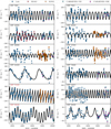 |
Fig. 2 Best Keplerian models for the 12 stars in the sample. The error bars of the RVs, representing the formal uncertainties of the measurements, are typically smaller than the markers. The identifiers of the two planet hosts, HIP 75458 and HIP 88048, are marked in red. Significant intrinsic RV jitter is present for most of the stars. |
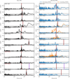 |
Fig. 3 Maximum likelihood periodograms of the RVs (left) and the residuals (right) after subtracting the best Keplerian model. As the SONG RVs are known to show spurious RV periodicity at a one-year period (Heeren et al. 2023), we plot the MLPs of the residual RVs excluding the SONG data in blue, while the periodograms including the SONG data are shown in orange. The FAPs of 5% (dashed), 1% (dash-dotted), and 0.1% (dotted) are plotted as gray horizontal lines. The identifiers of the two planet hosts, HIP 75458 and HIP 88048, are marked in red. Significant periodicity remains close to the strongest RV period after removing the best fit for many of the stars. |
4.3 Infrared test
Another approach that mostly emerged in the context of RV variability caused by star spots, is to test whether the RV signal is consistent at optical and infrared wavelengths. For star spots, as the contrast ratio between a cool spot and the stellar surface is much smaller in the infrared than in the optical, the RV variation introduced by a spot is generally expected to be smaller in the infrared compared to the optical (Desort et al. 2007; Huélamo et al. 2008; Reiners et al. 2010). As the photometric amplitudes of pulsating stars are known to be different in optical and infrared passbands as well (Percy et al. 2001), one can also expect the infrared test to be applicable in the context of suspected non-radial oscillations in RV data (Mitchell et al. 2013; Trifonov et al. 2014, 2015; Ortiz et al. 2016). In contrast, a planetary companion should induce a consistent RV signal in all wavelength regimes.
To first order, one can expect that the semi-amplitude K is the only changing parameter when fitting contemporary RVs taken in the VIS and NIR channels of CARMENES. We thus kept all parameters but K fixed from the previous modeling detailed in Sect. 4.1 and performed another dynamic nested sampling of the posterior distribution of K using only the CARMENES-VIS and CARMENES-NIR data, respectively. We adopted the mode of the distributions and derived the uncertainties by identifying the interval around the mode that encompasses 68% of the posterior samples, corresponding to a 1 σ credibility interval. We ensured the unimodality of each distribution by eye. We stress that we only compare the semi-amplitudes between the two CARMENES channels. These can, in some cases, be inconsistent with the determined semi-amplitudes using the whole data set, indicating that the RV signals are not stable over long time frames but can also be a consequence of sparse sampling.
We plot the results of the infrared test in Fig. 4. We find no significant differences between the amplitudes of the variations derived from the CARMENES-VIS and CARMENES-NIR data. For several of the very luminous stars, large error bars due to the large RV jitter and relatively few data points, sampling only two to three phases of the RV variations, reduce the informative value of the infrared test.
In Spaeth et al. (2024), we present a simulation of an l = 1, m = 1 non-radial oscillation that can reproduce the variations of the RVs and the activity indicators for the false-positive brown-dwarf host NGC 4349 No. 127 (Delgado Mena et al. 2018, 2023). Using the same simulation settings as in Spaeth et al. (2024) to derive hypothetical RVs in the CARMENES-VIS and CARMENES-NIR channels leads to semi-amplitudes KVIS = 249.6 m s−1 and KNIR = 257.6 m s−1, respectively, a relative difference of about 3%. This would, for most of the stars, be insignificant given the derived uncertainties in the presence of large stellar jitter. Thus, we conclude that the absence of significant differences between semi-amplitudes derived in the optical and the infrared cannot rule out a non-radial oscillation model.
We note that these findings are only valid for relatively small temperature variations employed in the simulations (here δTeff = 2.5 K), for which the chromatic limb-darkening correction dominates the chromatic behavior of the RVs. For larger temperature variations and other oscillation modes, the relative amplitude difference between infrared and visual RVs can change slightly compared to the presented case. However, our test simulations, including more extreme values and different oscillation modes, did not reveal any significant increase in the relative RV difference between the VIS and NIR channels, while maintaining photometric variations comparable to those of the stable stars in this sample. The infrared test is thus not sensitive enough to validate or disprove potential planets orbiting evolved stars.
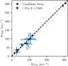 |
Fig. 4 Semi-amplitudes K from the CARMENES-NIR channel plotted against the semi-amplitudes in the VIS channel. We highlight the two secure planet hosts, ι Dra and ν Oph as red diamonds, while we show the planet candidates in blue. For ι Dra and ν Oph, only the inner orbital components are examined due to the short baseline of the CARMENES observations. |
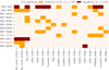 |
Fig. 5 Results of the linear correlation analysis. For each star we show the significance of the linear correlation between the activity indicator labeled on the x-axis and the respective RV data set. Red colors indicate significant (p < 0.1%) linear correlations, while orange colors represent tentative (0.1% ≤ p < 5%) correlations. The identifiers of the two planet hosts, HIP 75458 and HIP 88048, are marked in red. |
4.4 Analysis of the activity indicator time series
State-of-the-art, stabilized spectrographs, such as CARMENES, acquire a set of activity indicators simultaneous to the RVs. These activity indicators have proven to be very useful in the study of magnetic activity, as manifested in star spots or plages, in RV surveys that target main-sequence or low-mass stars. Delgado Mena et al. (2018,2023) have used activity indicators measured by HARPS successfully to rule out a number of exoplanets around cluster giants, showing that these indicators are also applicable to giant stars, for which magnetic activity is not necessarily the major concern.
4.4.1 Correlation analysis
In Spaeth et al. (2024), we show that the HARPS activity indicators for NGC 4349 No. 127, a known false-positive host (Delgado Mena et al. 2018, 2023), show peculiar correlations with the RVs. The CRX and the RVs are slightly positively correlated, while the dLW, FHWM, and contrast of the CCF have “closed-loop”, Lissajous-like correlations with the RVs. We further show that these are the correlations expected from an l = 1, m = 1 non-radial oscillation mode.
Motivated by these findings, we scanned the Lick Hα measurements and the CARMENES activity indicators for similar correlations with the RVs. By eye, we did not find any reliable closed-loop correlations in the sample. These could potentially be obscured by variations due to short-term p-mode oscillations, or the superposition of different modes (Spaeth et al. 2024). We further note that the RV amplitudes of the planet candidates in this sample are typically smaller than those of NGC 4349 No. 127, which makes the identification of such correlations more challenging.
Lacking indications for more complex correlations, we systematically tested the activity indicators and RVs for linear correlations. For each of the activity indicators and corresponding RV time series, we fitted for a linear relation. We assessed the significance of the resulting slope by performing a permutation test. That is, we uniquely permuted the pairs of variables N = 10 000 times and counted the number of simulated slopes m with |m| ≥|mreal|. The two-tailed p-value of the significance of the measured slope is then defined, following Ernst (2004) and Phipson & Smyth (2010), as
 (3)
(3)
We define correlations with 0.1% ≤ p < 5% as tentative correlations, while we regard p < 0.1% as significant. We computed p-values for all correlations without applying any threshold to the slope beforehand. The combined results of the linear correlation analysis can be seen in Fig. 5. We observe that only three of the stars, HIP 7607, HIP 84671, and HIP 89826 show any significant correlations. Only the former two show correlations in more than one indicator. That is surprising since we can find strong arguments against planets as the cause of the RV variations for a majority of the stars based on other metrics. In contrast to the case of NGC 4349 No. 127, we also do not find correlations between the CRX and the RVs in the CARMENES VIS channel for any of the stars.
On the other hand, we observe that all stars show at least one tentative correlation between the indicators and the RVs, even the two secure systems HIP 75458 and HIP 88048. Of course, these two systems could in principle also be contested, but given the extremely well-behaved RV variations of both systems with a large eccentricity in case of HIP 75458 and well-studied dynamical constraints for HIP 88048 (Quirrenbach et al. 2019), there are good reasons to assume that the planetary systems around these stars are real. In fact, it rather reflects the relatively poor performance of the simple linear correlation analysis.
This can be understood since searching for linear correlations in this way is sensitive to different kinds of variations of the activity indicators. These could, for instance, be linked to the known short-term p-mode pulsations or the stellar rotation and might be completely unrelated to any RV periodicity introduced by a planet. Such short-term variations in the activity indicators, combined with long-period RV variations of a different origin, can lead to spurious correlations. We thus conclude that a simple linear correlation analysis is not apt to differentiate between planets and intrinsic variations for the majority of the stars and argue in favor of more sophisticated metrics such as the periodogram analysis discussed in the following. We note that a combination of a well-behaved linear correlation with a finding of clear periodicity at the RV period could be helpful to remove the contribution of the intrinsic signal from the RVs (see, for instance, Robertson et al. 2014).
4.4.2 Activity periodogram analysis
To assess whether the activity indicators vary at periods linked to the established RV periodicity, we employ a periodogram search using MLPs. We present the results for two examples stars in Fig. 6. The full figures are shown in Figs. A.1 and A.2. These show the combined MLPs for all time series (RVs and activity indicators) of all instruments available for each star. Again, we overplot as gray horizontal lines the FAPs of 5% (dashed), 1% (dash-dotted), and 0.1% (dotted). We generally refer to peaks with 0.1% ≤ FAP < 5% to be tentatively significant, while we consider peaks with FAP < 0.1% to be significant. We further overplot the period for each Keplerian model (see Table 3) as thick, vertical, dark red lines and label their respective periods at the top of each panel. We also show the aliases of the RV period, computed with the strongest peak in each respective window periodogram, as thinner red lines, while we portray three harmonics and sub-harmonics of the RV period with lower opacity. The periodograms of the window functions were computed as discrete Fourier transforms and are plotted in the bottom panel. The strongest window peak for each instrument was detected in the range between 300 d and the baseline of the respective time series and is marked as the colored arrows on the x-axis of the panel. Following VanderPlas (2018), periodicity at the alias frequencies or the harmonics of the RV period should be regarded with caution. We note that many of the window functions show multiple peaks. However, we refrain from computing and plotting the aliases for each peak to avoid a cluttering of the plot. The results of the activity periodogram analysis are discussed on a star-by-star basis in Sect. 5.
4.4.3 DBSCAN cluster analysis
A useful way to summarize and detect associated periodicity in multiple CARMENES activity indicators is presented by Kemmer et al. (2025). Following this approach, we first detected all peaks by their FAPs and periods in the MLPs of all CARMENES activity indicators (both channels). We note that the process allows for multiple peaks of the same indicator time series to be detected. Next, we employed the DBSCAN (Ester et al. 1996) clustering algorithm available through scikit-learn (Pedregosa et al. 2011) on all identified peaks with FAP < 50%. We tested different settings for the DBSCAN parameter ϵ, which defines the maximum distance between two peaks to be considered neighbors, setting it to one-third of the width of the peaks in the periodogram as estimated by δ f = (tmax − tmin)−1. We found this value to provide good results at the long periods of interest in this work. We limited the identified clusters to have at least three peaks, with at least one of the peaks having tentative (FAP < 5%) significance. We further limited the cluster search to periods longer than 100 d, to only target periodicity close to the dominating, long-period variations of the RVs.
The results of the cluster analysis are plotted for two example stars in Fig. 7 and for the full sample in Fig. B.1. These are discussed in detail on a star-by-star basis in the following. In general, we find that a majority of the stars whose RV variations are likely intrinsically induced show clustered activity periodicity close to the main RV period. These findings are mostly contributed by the VIS channel, which, however, also has several additional line indicators in contrast to the NIR. Somewhat unsurprisingly, we often find that the line shape indicators (dLW, BIS, contrast and FWHM of the CCF) vary at similar periods and thus form activity clusters. However, we often also find contributions to the same clusters from other indicators, including the CRX and the chromospheric indicators targeting the Hα and NaD lines.
5 Combined results for individual stars
In this section, we discuss the results star-by-star, aiming to determine whether planets or intrinsic variations are causing the observed RV variations.
5.1 HIP 7607
The horizontal branch giant HIP 7607 (υ Per) shows strong and clearly significant RV periodicity close to the fitted period of P = 523.3 d in the Lick and both of the CARMENES data sets in Figs. 6 (left) and A.1 (top left). For both instruments, periodicity can also be found at the respective alias periods (thinner, red lines). We note that the peaks in the Lick RV MLP (P = 538 d, see also Hekker et al. 2008) and the CARMENES RV MLPs (both P = 508 d) are slightly offset. However, given the relatively short baseline of the CARMENES observation and the width of the peaks, this difference cannot be regarded as significant.
Examining the activity indicators in Fig. 6, we find a number of peaks with tentative significance in the vicinity of the RV period in the CARMENES VIS channel. The most significant peak (FAP ∼ 0.1%) is contributed by the NaD2 line at P = 491 d, slightly offset from the RV period. Further tentative peaks close-by can be found by the dLW, contrast, and BIS indicators. Further periodicity in the activity indicators is also present close to the alias period of the fitted RV period. The DBSCAN cluster analysis in Figs. 7 (left) and B.1 (top left) reveals two clusters of activity variability centered at P = 478 d (cyan) and P = 572 d (orange). Together, the activity indicators clearly cast doubts on the planetary nature of the RV signal.
The doubts are further strengthened by several significant correlations present between the activity indicators and the RVs, as evident from Fig. 5. However, as discussed in Sect. 4.4.1, the overall mixed results of the correlation analysis reduce the informative value of such correlations. The final and strong argument against the planetary nature of the RV signal comes from analyzing the residual RVs. As can be seen in Fig. 3, there is significant periodicity left at P = 441 d, P = 489 d, P = 614 d, and other more distant periods. Similar systematics in the residuals of the Lick data of HIP 7607 have been noted by Quirrenbach et al. (2011). Trying to explain this additional periodicity with another orbital companion requires a minimum mass exceeding 1 MJup, which would make the proposed system unstable. It is thus much more likely to be a manifestation of a multi-periodic incoherent type of RV variation that is linked to intrinsic processes.
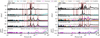 |
Fig. 6 Maximum likelihood periodograms for two example stars. The top panel for each star portrays the combined RV MLP. In the remaining panels, we show the MLPs of the RVs (black) and activity indicators (see legend) for each instrument. The FAPs of 5% (dashed), 1% (dash-dotted), and 0.1% (dotted) are plotted as gray horizontal lines. The bottom panel shows the instruments’ window functions derived as discrete Fourier transforms. The thick, red, vertical line indicates the period of the Keplerian fit (see Table 3). The alias periods, corresponding to the most significant peak in the respective window function, are shown as thinner lines. The positions of these window peaks are marked with colored arrows in the bottom panels. Notably, the CARMENES VIS and NIR window functions largely overlap. Additionally, we display the harmonics and sub-harmonics of the period of the Keplerian fit as red lines with lower opacity. The full figures are shown in Figs. A.1 and A.2. |
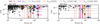 |
Fig. 7 Example results of the DBSCAN clustering algorithm for two stars. In each panel, all identified peaks in the MLPs of the CARMENES activity indicators are shown as filled circles. Arbitrarily colored circles represent activity peaks assigned to clusters by DBSCAN, while gray circles indicate peaks that are not part of any cluster. The larger, empty circles indicate the center periods and FAPs of the clusters. We further overplot the FAP levels of 5% (dashed), 1% (dash-dotted), and 0.1% (dotted) as horizontal gray lines, and the fitted RV period (thick), its aliases (thin, based on the VIS window function), and harmonics (lower opacity) as vertical red lines. Furthermore, for stars where individual instruments exhibit a strongest period that deviates from the fitted period by at least 10% (restricted to 100 d < Pmax < 5000 d), we overplot the strongest RV period detected in the MLP of the respective instrument using vertical, colored lines specified in the legend. The full figure is shown in Fig. B.1. |
5.2 HIP 7884
One star that highlights the usefulness of the periodogram analysis of activity indicators is HIP 7884 (ν Psc), a bright (V = 4.4 mag) K3 giant star likely located on the RGB (see Table 1). Focusing first on the Lick RV MLP in Figs. 6 (right) and A.1 (top right), one can clearly see the dominant and highly significant peak in the RV periodogram at P = 628 d. However, in the CARMENES RVs (third and fourth panels) no significant periodicity can be found at that period, revealing peaks at P = 418 d, P = 549 d, and P = 1028 d in the VIS instead, with peaks in the NIR at similar periods. As a consequence, the MLP of the combined RVs (top panel) reveals a complex structure, reducing the significance of the most prominent peak compared to the Lick data set alone, and introducing further peaks close-by. These findings likely indicate that the periodic variation present in the Lick data set, is not present in the CARMENES RVs, which cover a more recent time baseline. Analyzing the residual periodogram in Fig. 3, one can see this behavior manifested as a second peak, a mere 30 d distant in period space.
Examining the available activity data in Figs. 6 and 7, one can find a significant peak of the Lick Hα measurements at the period of the Lick data, as well as peaks of the dLW and the contrast of the CCF of the CARMENES VIS channel, which are both evident at the RV period and at its alias frequencies (thinner, red lines). Thus, a planetary origin of the RV periodicity can be excluded. The activity peaks in the CARMENES data appear to belong to a cluster (including tentative peaks from the CARMENES Hα indicator and the BIS) centered very close to the fitted period (Fig. 7). One further observes two clusters centered at the two long-period aliases of the RV period. Despite these significant detections of activity variations at the RV period, there are only tentative correlations present in Fig. 5. These include the two time series of Lick Hα measurements, as well as the Hα indicator derived from the visual CARMENES channel. Each of the Hα time series shows a tentative positive correlation with the RVs. The FWHM of the CCF of the NIR channel is also tentatively positively correlated with the RVs.
Combining all the above findings, these observations make HIP 7884 another example of a giant star whose measured RVs, when viewed in isolation, seemed to be consistent with an orbital companion for over 12 years. However, by using a much longer RV baseline and acquiring reliable activity indicators, its cause can decisively be concluded to be of intrinsic origin.
5.3 HIP 16335
One of the most interesting stars within the sample is HIP 16335 (σ Per), which was published to host a planetary companion with minimum mass mp sin(i) = 6.5 ± 1.0 MJup in a P = 579.8 ± 2.4 d orbit by Lee et al. (2014). The authors used RV data from the Bohyunsan Observatory Echelle Spectrograph (BOES) at the Bohyunsan Optical Astronomy Observatory (BOAO) in Korea, along with activity indicators derived from the Ca II H line, and studied the bisector variations of the Ni I 6643.6 Å line. They find no periodicity or correlations with the RVs. We include the BOAO data set as published by Lee et al. (2014) in this analysis.
While the peaks in the BOAO and Lick RV MLPs (Fig. A.1), which are roughly contemporary, are clearly apparent and strongly significant, the RVs in the CARMENES visual channel show a much less significant peak, which is further slightly offset to P = 609 d. The infrared RVs of CARMENES show a strong peak at P = 599 d. However, two strong peaks close to the originally published planet period emerge in the CARMENES-VIS activity indicator MLPs: both the CRX and the BIS of the visual channel have significant peaks at P = 559 d and P = 565 d, respectively, close to the originally published planet period P = 579.8 ± 2.4 d (Lee et al. 2014). We further note additional peaks of the VIS Hα indicator, the CCF contrast, and the BIS in the vicinity of the alias and harmonic periods of the RVs.
The DBSCAN clustering algorithm presented in Fig. B.1 shows two adjacent clusters neighboring the RV period, which shows that there is further, tentative periodicity of activity indicators close-by. We note that the two significant peaks in the CRX and BIS are attributed to the cluster centered at P = 527 d (green).
The strong evidence against the planetary companion is further enhanced when looking at the residuals of the RV fit in Fig. 3. After subtracting the best planet fit, significant variability with a period P=561 d remains, a mere 37 d offset from the fitted period. This additional variability can hardly be explained by a second orbital companion fulfilling stability constraints. Instead, we interpret it to be a sign of a non-constant periodicity or amplitude of the RV signal. Altogether, these findings strongly argue against the planetary nature of the RV signal of HIP 16335 and thus contradict the findings by Lee et al. (2014).
5.4 HIP 38253
HIP 38253 (HD 63752) is the most luminous star in the sample and shows relatively large-amplitude RV variations with K ∼ 148.1 m s−1. First hints of an intrinsic origin have already been found by Hekker et al. (2005). Examining the MLPs in Fig. A.1 confirms these findings.
The Lick RVs show a dominant peak at P = 619 d, with a small side-lobe and secondary peak at P = 766 d. In contrast, the SONG data set, bridging between the Lick RVs and the most recent CARMENES observations, does not show the same periodicity but instead a most dominant peak at P = 416 d, and further power at longer periods. This shorter-period peak is, however, no longer present in the CARMENES data set, which rather shows two less significant peaks at P=631 d and P = 874 d. It is thus apparent that RV variations at inconsistent periods are present in data sets spanning different time windows. This is also evident from the complex structure of the combined MLP in the top panel. The nested sampling algorithm reveals Pfit = 735.3 d to be the modal value of the period posterior distribution, which shows a slight bimodal structure. It is clear that this RV variation is not stable and cannot be caused by a planetary companion, which would be expected to be consistently present in all data sets. This is also evident from the rather unsatisfying mono-periodic fit to the RV data in Fig. 2.
Due to this multi-periodicity in the RV data, the activity time series is more challenging to interpret. Taking a look at the clustering results in Fig. B.1, it is evident that a strong cluster of significant activity indicator periodicity is present very close to the RV period present in the SONG data set (marked as the orange line). The most dominant peaks stem from the line shape indicators (dLW, FWHM and contrast of the CCF, BIS) in the VIS, but also partially in the NIR. There are further tentative peaks by the Hα and CaIRT2 lines in the vicinity, as apparent from Fig. A.1.
Close to the strongest period in the Lick RVs (P = 619 d, blue line) is another, less significant, cluster of activity variations, apparent both in the line shape indicators in VIS and NIR, as well as the Hα line, and the CRX in the VIS. Finally, there appears to be another cluster of activity variations present at somewhat longer periods. While there is no significant peak exactly at the fitted RV period, it appears that each tentative peak of the CARMENES RVs is accompanied by at least tentative variability in the activity indicators.
As noted for the whole sample, the correlation analysis reveals only tentative correlations between the activity indicators and the RVs. This result is surprising given the strong support for an intrinsic origin of the RV variations. It strengthens our conclusion that a simple linear correlation analysis cannot properly capture the complexities of the relations between activity indicators and RVs for giant stars. It can likely be understood as a consequence of the multi-periodic nature of the variations in both the RVs and the indicators. Looking at the residual RVs in Fig. 3, it is clear that significant residual periodogram power is present in the vicinity of the fitted RV period, confirming this multi-periodicity. We conclude that the RV variations of HIP 38253 are of intrinsic origin.
5.5 HIP 46390
Somewhat similar to HIP 38253 is the behavior of the very bright (V = 1.97 mag) giant HIP 46390 (Alphard, α Hya, HD 81797), although the amplitude of the variations is much smaller (K ∼ 47.3 m s−1). Again, the strongest peak in the Lick data set (2000–2011) at P = 524 d is not dominant in the later SONG observations (2015–2022), which have the strongest periodogram peak at P = 306 d (see Fig. A.1). The most recent CARMENES observations (2016–2023) show their most significant periodicity at P = 422 d. As for HIP 38253, this also rules out the presence of a stable planetary system for HIP 46390, which coincidentally is the second most luminous star in the sample. As mentioned in Sect. 4.1, the nested sampling algorithm shows multimodal posterior distributions with different periodicities being picked up in different runs of the algorithm. The final model used in this work is mostly dominated by the Lick RVs, with the SONG RVs showing a clear phase shift in a phase-folded RV plot.
Subtracting the best Keplerian model from the RVs and examining the residual periodogram in Fig. 3, we find that there remain several significant peaks when including the SONG data (orange). Removing the SONG data set from the analysis, we find that there is residual periodicity with significant peaks at P = 422 d and P = 451 d (blue periodogram). Thus, the best model cannot remove all variability close to its modeled period.
Examining the activity indicator periodograms in Fig. A.1 and their clustering in Fig. B.1, we find a significant peak by the CARMENES-VIS Hα indicator (FAP = 0.03%) close to the Lick period. This activity peak is attributed to a small cluster, jointly with a tentative peak by the contrast of the CCF in the NIR channel, centered at P = 515 d. Close to the SONG RV period (P = 306 d, orange line in Fig. B.1) that dominates the combined RV periodogram, we find a close cluster at P = 325 d of significant and tentative peaks mostly contributed by the dLW and contrast of the CCF in the VIS, as well as the NaD2. Thus, the dominant RV periodicity in the SONG RVs also seems to be present in the variations of the spectral lines as measured by CARMENES. Finally, we observe a tentative peak by the dLW close to the most prominent RV peak in the CARMENES data set. As with many other stars, we find only tentative correlations between the Hα indicator, dLW, and CCF contrast on the one hand, and the RVs on the other. Taken together, there is overwhelming evidence that the RV variations observed for HIP 46390 are of intrinsic origin, with changing periodicity on timescales of a quarter of a century.
5.6 HIP 47959
HIP 47959 (18 Leo, HD 84561) is another relatively luminous star within our sample. Examining Fig. A.1 (bottom right panel), the RV variations can again be shown to have varying periodicity in different time windows. While the Lick RVs show dominant periodicity at P = 611 d, the SONG data taken at later epochs have a shifted peak at P = 495 d, with a secondary peak at P = 654 d, close to the Lick RVs. The former periodicity dominates the RV period determined through the nested sampling (P = 481.3 d). The CARMENES data do not yet show a significant peak but have their strongest periodicities at P = 580 d in both channels. The combination of all available RV data then leads to a relatively complex periodogram apparent in the top panel. Following from this multi-periodic behavior, one can find a number of significant peaks close to the removed period in the residuals (Fig. 3).
Adding to these strong arguments against a planetary nature of the RV variations, we can find a number of tentative peaks in the activity indicators of the CARMENES channels (mainly the VIS), with some periodicity (both significant and tentative) present in the Lick Hα indicator at somewhat shorter periods. Analyzing these using the DBSCAN clustering algorithm in Fig. B.1, we find a strong cluster at P = 478 d, coinciding closely with the fitted RV periodicity that was mainly dominated by the SONG RVs. It is thus evident that the RV variations are again of intrinsic origin. Despite these indications of intrinsic RV variations, only two tentative correlations are found between the activity indicators and the RVs, namely, for BIS and CaIRT2. This illustrates again the shortcomings of the correlation analysis.
5.7 HIP 64823
HIP 64823 (HD 115478) stands out within the sample as the candidate star with the longest-period RV variation, with a period of P = 2878.1 d. It is likely (P = 90%) located on the RGB (Stock et al. 2018). HIP 64823, unfortunately, was not part of the SONG observations, such that only Lick and CARMENES data are available. The baseline of the latter is furthermore a little shorter than one whole period of the RV variations such that an exact determination of the RV periodicity in the CARMENES data is not yet possible. Nevertheless, an increase of the likelihood at the period of the Lick RVs can be seen in Fig. A.2.
Analyzing the activity indicators both in Figs. A.2 and B.1 suffers from the same limitation. We do find a tentative peak of the NaD 2 line at P = 1940 d, which, however, closely coincides with a peak in the window function of the CARMENES observations (bottom panel). Apart from that, there is (so far) no indication of any significant periodicity at periods similar to the RV period in either plot. While we cannot rule out a long-period activity variation with certainty, we conclude that the NaD2 variation is likely a consequence of the sampling of the observations.
The linear correlation analysis reveals two tentative correlations between the RVs and the contrast of the CCF in both the VIS and NIR channels. The p-values of the correlations are 3.3%, and 3.2% in the VIS and the NIR, respectively. However, we note that the correlation between the contrast of the CCF and the RVs is of opposite sign in both channels. That is, it is anti-correlated in the VIS, while it is positively correlated in the NIR. Combined with our general finding that the correlation analysis seems to be relatively ineffective for the giant stars in this work, we find it likely that these correlations are mostly a consequence of large uncertainties in the determination of the CCF parameters coupled with a relatively small number of measurements, as well as short-term jitter or the potential presence of intrinsic variations at shorter periods (see Sect. 6).
Analyzing the residuals in Fig. 3, we find the closest significant periodicity at P = 410 d, with a slight secondary peak at P = 436 d. In contrast to the previous stars, this additional periodicity does not seem to be a sign of a changing periodicity of the dominating period. Overall, we conclude that the CARMENES data available so far do not argue against the planetary nature of the RV periodicity. However, due to the insufficient baseline of the CARMENES observations, we cannot conclusively exclude any connection to intrinsic processes. We thus conclude hat HIP 64823 remains a good planet candidate and examine the Keplerian model in more detail in Sect. 6.
5.8 HIP 73620
The second least luminous star in the sample, HIP 73620 (110 Vir, HD 133165), has the smallest RV variations of the sample with semi-amplitude K ∼ 20.3 m s−1, only marginally larger than the estimated and expected jitter σjit ∼ 13.3 m s−1. The star is located in the red clump (Alves 2000; Laney et al. 2012). Examining Fig. A.2, one can observe a rather complex combined periodogram structure with the period P = 512.5 d being picked up by our nested sampling approach. This period coincides with the dominant periodicity in the Lick data set. The CARMENES RVs show a slightly offset peak at P = 554 d in the VIS channel, and at P = 547 d in the NIR. In the vicinity, we further observe several peaks present in the CRX and dLW of the VIS channel with varying levels of FAPs.
When analyzed using the DBSCAN algorithm in Fig. B.1, we find a cluster of peaks centered at P = 539 d, very close to the RV period. We note, however, that two of the peaks each stem from the CRX and dLW indicators. We further observe four tentative correlations for dLW, FWHM, and NaD1 in the VIS, as well as between the BIS and the RVs in the NIR. Using the period information from the RV residuals in Fig. 3, we find that subtracting the best fit reveals periodicity close-by at P = 597 d, P = 544 d, and P = 421 d, with the central period closely coinciding with the CARMENES periodicity. The latter finding indicates that the shift of the periodicity in the CARMENES RVs is likely real and not a consequence of insufficient sampling of the phase curve. Overall, we conclude that the relatively small RV variations (within the context of this sample) of HIP 73620 are most likely caused by intrinsic variations instead of a planetary companion. Nevertheless, the star would benefit from continued observations to increase the temporal baseline and acquire additional measurements of activity indicators before a firm conclusion can be drawn.
5.9 HIP 75458
Next, we examine HIP 75458 (ι Dra, HD 137759), one of two published planet systems hosting a super-Jovian exoplanet in a 511 d, very eccentric orbit (Frink et al. 2002). The RVs further show a long-period trend (Zechmeister et al. 2008; Kane et al. 2010) attributed to a further-out brown-dwarf companion (Hill et al. 2021). The star was observed using SONG and added to the CARMENES sample in 2021.
Examining the periodograms in Fig. A.2, one can observe that the strong RV periodicity at P = 510.9 d is consistently present in all data sets. Due to the very eccentric orbit of ι Dra b (named Hypatia by the IAU) and the sinusoidal nature of the periodogram analysis, one can identify clear and significant periodicity also at the harmonics and aliases of the RV period. Examining the activity indicators, there is no strong peak at the planet period. We observe tentative periodicity of the NaD1 and NaD2 lines at P = 402 d and P = 349 d, respectively. However, we note that these periods are also in proximity to one year, which suggests a connection to variable observing conditions or telluric contamination. This suspicion is reinforced by the DBSCAN clustering algorithm (Fig. B.1), which detects a cluster of peaks (two of which are insignificant) centered at P = 368 d. We thus find no evidence against the planetary hypothesis from the activity time series analysis.
As mentioned in Sect. 4.4.1, we find tentative correlations (see Fig. 5) between the RVs and the CaIRT1 line in the VIS, as well as the dLW, FWHM, and contrast of the CCF in the NIR, with the latter having a p-value p = 0.3% close to the significance threshold. It is noteworthy that all three indicators that show these tentative correlations in the NIR are based on similar variations of the spectral line shape (see, for instance, Zechmeister et al. 2018), and are thus not entirely independent. As discussed in Sect. 4.2, we find two significant peaks in the residual periodogram, excluding the SONG RVs, at P = 407 d and P = 634 d. Both are much less significant than the initial peak caused by the orbital companion and lie in proximity to alias periods of the Keplerian period and the structured, combined window function. We thus suspect that these are a consequence of the large eccentricity of the orbit of ι Dra b, which might be imperfectly constrained by the orbital fit.
Overall, we observe some noteworthy features in the activity indicator and residual analysis of ι Dra. However, individually we regard none of these as strong arguments against a planetary nature of the RV signal. Moreover, the Keplerian orbit has a very high eccentricity (e ∼ 0.71), which can hardly be mimicked by, for instance, non-radial oscillations. It is further extremely well determined and fulfills all stability constraints (Hill et al. 2021). The star is furthermore the least luminous star in the sample (L ∼ 57 L⊙) with radius R ∼ 12 R⊙, placing it relatively far away from the region of suspicious planet detections identified by Reichert et al. (2019) and Döllinger & Hartmann (2021). We therefore have no reason to question the existence of ι Drab. The results in this section rather emphasize that none of the metrics, particularly the correlation analysis, provide definitive conclusions regarding the existence of a planet responsible for the RV signal.
5.10 HIP 84671
HIP 84671 (66 Her, HD 156681) belongs to the most luminous stars in the sample with L ∼ 472 L⊙. It shows similar behavior to the two even more luminous sample stars, HIP 38253 and HIP 46390. While the RV periodicity at P = 447.2 d is strongly present in the Lick data set (see Fig. A.2), it is not properly picked up in the CARMENES RV MLPs (black lines). The strongest peak in the vicinity of the fitted period is instead caused by the CRX in the VIS at P = 423 d, with further tentative peaks close to the alias periods from the CRX and the Hα line. We further find a long-period signal at P = 1105 d in the VIS (and P = 1094 d in the NIR) to be the most significant peaks in the CARMENES RVs. This peak is accompanied, however, by an even more significant peak in the Hα indicator. These are not present in the longer Lick time series. Finally, we find a significant peak in the Lick Hα time series, within the peak width of the peak in the Lick RV MLP. Combining the peak information into the cluster analysis in Fig. B.1, one can observe a cluster centered at 432 d (very close to the fitted period), with another longerperiod cluster potentially linked to the long-period RV variation present in the CARMENES data.
The Hα variations in both Lick and CARMENES are also significantly correlated with the RVs, albeit likely linked to different periodicity in the different instruments. These correlations are all with a positive sign, strengthening the significance of the finding. HIP 84671 thus appears as one of the few stars for which the correlation analysis can provide useful additional information. Subtracting the Keplerian model leads to residuals with additional significant periodicity at P=470 d and P = 506 d. Thus, we conclude that the RV variations with a large semi-amplitude K ∼ 220 m s−1 are of intrinsic origin.
5.11 HIP 88048
The other published planetary system in our sample orbits HIP 88048 (ν Oph, HD 163917) and consists of two brown-dwarf companions identified by Quirrenbach et al. (2011, 2019). The MLP analysis in Fig. A.2 reveals no tentative or significant peaks in the vicinity of the RV period of ν Oph b (P = 529.9 d), and likewise, no significant clusters are detected in Fig. B.1. We do observe a number of insignificant peaks by the Lick Hα, and CARMENES Hα, NaD1, and CaIRT2 indicators close to the one-year period.
The period of the outer brown-dwarf companion at P = 3173.4 d is much longer than the baseline of the CARMENES observations. Therefore, no reliable conclusions can be drawn from the CARMENES activity indicators for that period. We do find, however, a rise of the likelihood for the Lick Hα indicator at even longer periods, which does not seem to be directly connected to the RV period of ν Oph c. This long period is at the limit of the baseline of the Lick observations (4009 d) and could also be linked to aging effects of the Lick CCDs. This trend of the Hα indicator is likely also causing the two tentative correlations between the Lick Hα indicators and the RVs (see Fig. 5), with p-values of p = 1.8% and p = 2.7% for the first and second Lick CCD, respectively. No correlations are detected between the CARMENES activity indicators and the RVs.
After removing the two-planet model from the RVs, we do not find any significant power close to the orbital periods in Fig. 3. Overall, we thus conclude that there are no indications in the CARMENES data that argue against the real nature of the inner brown-dwarf companion, while the outer is still outside the baseline of the CARMENES observations.
5.12 HIP 89826
HIP 89826 (κ Lyr, HD 168775) is the second star among the planet candidates that stands out due to the relatively long-period nature of the RV variations which have a fitted period of P = 1642.6 d. Looking at Fig. A.2, these are clearly apparent in the Lick data set, while they are (still) insignificant in the CARMENES-VIS RVs and only tentatively present in CARMENES-NIR. However, the baseline of the CARMENES RVs is only a few hundred days longer than the fitted period, which is a potential reason for the lack of significance in the CARMENES measurements. The semi-amplitude of the RVs, K ∼ 32.5 m s−1, is relatively small compared to the average of the sample and compared to the jitter σjit = 12.8 m s−1 likely caused by short-term pulsations and expected for this star. This can provide an additional explanation for the lack of periodicity in the VIS data set. Finally, the measurements (see Fig. 2) do not ideally sample the phase curve of the proposed planet due to a gap in the CARMENES data in 2019 and 2020.
Analyzing the activity indicators in Fig. A.2, we find no significant periodicity at the Keplerian period. We find two tentative peaks by the CARMENES-NIR CRX and BIS close to the second harmonic of the RVs, which also form a small cluster with another tentative peak of the CARMENES-VIS CRX indicator centered at P = 781 d (see Fig. B.1). Another tentative cluster of peaks can be found close to the fourth harmonic of the Keplerian period.
We further find a significant correlation between the RVs and the CRX in the NIR channel (see Fig. 5), likely linked to the tentative periodicity of the CRX at the second harmonic of the RV period. We also find a tentative correlation (with p-value close to being significant) between Hα and the RVs using the second Lick CCD. Removing the Keplerian fit from the RVs and analyzing the residual MLP in Fig. 3 does not reveal any residuals peaks in the vicinity.
Altogether, we conclude that the CARMENES activity indicators so far do not decisively rule out a planet causing the RV variations. Nevertheless, since the long-period signal of the RV variations is not yet properly picked up by the CARMENES data given the sizable stellar jitter, we conclude that continued observations would be necessary to reveal its origin.
5.13 Summary of the results
Overall, we can find strong reasons to suspect that the RV variations of seven out of the ten planet candidates are caused by intrinsic processes. These are the stars HIP 7607, HIP 7884, HIP 38253, HIP 46390, HIP 47959, HIP 84671, and, notably, the published planet host HIP 16335 (Lee et al. 2014). We further lean toward an intrinsic origin of the RV variations of HIP 73620. The CARMENES activity indicators so far do not rule out a planetary origin of the long-period RV variations of HIP 89826, but continued monitoring is necessary to draw firm conclusions. For HIP 64823, we favor the planet hypothesis, which is examined in more detail in Sect. 6.
For the two comparison stars, HIP 75458 and HIP 88048, we find some tentative correlations between activity indicators and the RVs, which likely highlights the limitations of this analysis. We do not find any significant periodic signals in the activity indicators which would argue against the existence of the orbital companions. For HIP 75458, we note some residual periodicity, which is likely due to the large eccentricity of the orbit.
We generally conclude that testing for linear correlations does not provide strong and reliable insights for distinguishing between planets and intrinsic processes. We further find that the infrared test is not sensitive enough in the presence of large RV jitter and relatively little data. Overall, we find that a very long baseline of RV measurements is necessary to detect the subtle differences between the intrinsically induced variations and real planets. A detection of different periods in different time windows, as well as an analysis of the residual RVs can provide the strongest clues toward the origin of the RVs. We note that the most luminous stars in the sample (HIP 38253, HIP 46390, and HIP 84671) seem to show the strongest signs of changing periodicities in data sets taken at different epochs and with different instruments. A complementary periodogram analysis of activity indicators can often confirm these signals to be of intrinsic origin. We cannot identify any indicator that would consistently be more sensitive than the others in our analysis.
6 The long-period planet candidate HIP 64823
6.1 Radial velocity modeling
In Sect. 5, we find that the long-period planet candidate HIP 64823 stands out from the rest of the sample as there are currently no indications from the activity analysis or the RV residuals that argue against a planet causing the RV periodicity. Furthermore, the RV variation with a period P = 2878 d is, by far, the longest among the planet candidates, and far outside the typical range of periods detected to be false positives, which is several hundred days.
The best one-planet model presented in Fig. 2 has stellar jitter σjit = 36.7 m s−1, which lies between the jitter estimates σjit = 18.0 ± 2.3 m s−1 (Kjeldsen & Bedding 1995) and σjit = 50.8 ± 8.8 m s−1 (Kjeldsen & Bedding 2011). Thus, we tested whether some residual periodic signal was absorbed into the jitter estimate in the one-planet model.
Examining the RV residuals in Fig. 3, we find significant periodicity at several periods, with the most prominent peaks consisting of two blended peaks with maxima at P = 410 d and P = 436 d, as well as other peaks at P = 85.6 d and P = 15.7 d. We tested a 2-planet model (2P) with a uniform period prior  (300 d, 500 d) for the inner planet, trying to capture the most significant periodicity. We give the full set of priors in Table C.2. The resulting model attributes a period P = 438 d to the inner companion. We compare the Bayesian evidence resulting from the nested sampling run and find a moderate improvement of Δ
  = 3.41(Δ BIC = −2.8; Trotta 2008) compared to the oneplanet model. We further find that the estimated RV jitter is only reduced to σjit = 31.5 ± 3.6 m s−1, still exceeding the lower estimate by Kjeldsen & Bedding (1995).
Examining the activity MLPs in Fig. A.2, however, we find several peaks of the activity indicators in the period region between 100 d and 500 d, with a tentative peak of the CaIRT2 line at P = 397 d, not far off the residual period of the RVs or the period of the inner planet in the two-planet model. We thus suspect that the periodicity at shorter periods might be linked to stellar activity or another form of intrinsic variability and attempt to model it using a Gaussian process (GP) regression model as implemented via the celerite (Foreman-Mackey et al. 2017) package included in the Exo-Striker. While cool spots such as those commonly found for low-mass dwarfs are practically ruled out by the low level of photometric variability (Hpscat ∼ 0.005 mag), other sources of intrinsic variations, such as variable levels of convection or long-period stellar oscillations, are not well understood for giant stars. We thus attempted to model these variations with a commonly used but flexible rotational kernel defined by Foreman-Mackey et al. (2017). The kernel is characterized by the amplitude of the covariance B, the kernel period P, the coherence timescale L representing the decay of correlations over time, and a dimensionless factor C that adjusts the relative contributions of the periodic and constant terms.
In initial tests, using a joint model combining the contributions of the outer planetary candidate and the GP (1P+GP) and broad priors, we found that the GP mostly preferred a kernel period P ∼ 460 d but with small coherence timescales, which tended to overfit the short-term noise inherent to the RVs of the giant due to p-mode pulsations. Similar to Stock et al. (2023, their Fig. 2), we observed a triangular shape in the L−P plane of the posterior samples. That is, we detected many samples having small L but spanning a large range of periods P, as well as a distinct branch of solutions close to P ∼ 460 d extending to larger values of L. We thus restricted the lower limit of the prior on L to 450 d and clipped this plateau.
We selected a rather constrained prior on the factor C ( (0, 1)), expecting the oscillating component to have a significant contribution. The final 1P+GP model is presented in Fig. 8 (top left), decomposing the contributions of the planet (top right), and the contribution of the GP (bottom left). We find that the Bayesian evidence Δ
  = 33.3 and Δ BIC = −72.7 of the 1P+GP model are strongly favored compared to the one-planet model, as well as the two-planet model. We tested that the period prior has an insignificant effect on the Bayesian evidence computed for model comparison with the two-planet model. The residual RV scatter modeled as jitter results in σjit =
  m s−1, which is consistent with the jitter estimate by Kjeldsen & Bedding (1995). The determined kernel period is PGP =
  d. Given the strongly favored 1P+GP model compared to the two-planet model, we find the suspicion justified that the variability at P ∼ 400 d is caused by intrinsic variations rather than another planetary candidate. We give the mode of the posterior distributions in Table 4 and provide the corner plot of the posterior samples in Fig. D.1. The GP parameters are not very well constrained. We specifically find a broad distribution for the hyperparameter CGP. We stress that we regard HIP 64823 as a planet host candidate due to the insufficient time baseline of the CARMENES observations that cannot entirely rule out that the long-period variations could be caused by intrinsic processes.
6.2 Stacked Bayesian GLS analysis
Another test to distinguish RV periodicity caused by planets from those caused by intrinsic processes is proposed by Mortier & Collier Cameron (2017). The idea is to test whether the periodogram power of an RV signal increases by adding new data points as expected from a long-lived, coherent periodic signal. Mortier & Collier Cameron (2017) use stacked Bayesian GLS (SBGLS) periodograms based on the formalism by Mortier et al. (2015). The S-BGLS periodograms have been used successfully to distinguish stellar activity from planets around main-sequence dwarfs or T Tauri stars (see, for instance, Zaire et al. 2024; Von Stauffenberg et al. 2024; Burt et al. 2024; Dalal et al. 2024; Dreizler et al. 2024). The S-BGLS and similar tests have also been successfully applied to rule out the orbital companions around the giant stars Aldebaran (Reichert et al. 2019) and Sanders 364 (Zhou et al. 2023).
Results of the 1P+GP nested sampling modeling.
However, similar to Zhou et al. (2023), we find the color map representation of the S-BGLS (see Fig. 1 in Mortier & Collier Cameron 2017) somewhat subjective to interpret. Instead, we opt for an approach similar to that by Hatzes (2013), Reichert et al. (2019), and Zhou et al. (2023), as also proposed by Mortier & Collier Cameron (2017). That is, we plot the growth of the significance of the periodic signal, as expressed by the ratio between the amplitude of the sinusoidal A, derived by the circular S-BGLS periodogram, and its uncertainty σA, as a function of the number of data points N that have been added in sequence. The S-BGLS power was evaluated at the period of the best Keplerian model. These are portrayed in Fig. 9, as the blue lines. Due to the presence of secure long-period orbital companions in the HIP 75458 and HIP 88048 systems, we prewhitened the data sets for these stars by subtracting the contributions of the respective other orbital companions in the analysis. For HIP 88048, we also plot the growth of the signal of HIP 88048 c in orange. For HIP 75458, we omit plotting the change of the significance of the outer long-period companion, as its phase curve is only fractionally sampled.
As can be seen for both published planet hosts, HIP 75458 and HIP 88048, the significance of A can drop significantly in parts of the data set. However, these can be the results of an inadequate sampling of the RV phase curve in the presence of stellar jitter. For HIP 75458, for instance, the SONG spectrograph took numerous spectra in subsequent nights. Coupled with the eccentric orbit of HIP 75458 b and the sizable stellar jitter, these spectra in practice mostly contribute stellar “noise” and reduce the significance of the determined RV signal. This also helps one understand why the color maps of the S-BGLS analysis can sometimes be misleading for giant stars.
To study how the significance of A would evolve if the Keplerian model can adequately describe the data, we simulated 1000 realizations of the Keplerian model evaluated at the epochs of the real spectra and adding a Gaussian noise component with the standard deviation set to the RV jitter of the star. The latter was also used as a white noise component for the weights to compute the S-BGLS (see Mortier & Collier Cameron 2017). These simulations are plotted as the gray lines. As one can see for both HIP 75458 and HIP 88048, the simulated significances follow the real data very closely, including the drop of the significance in certain parts of the relation. We note the change of the significance of A for HIP 88048 c (orange) is initially very noisy and behaves slightly differently than the simulated relations. However, this can easily be explained by the long-period nature of the orbit, which has the longest period among all systems apart from HIP 75458 c, as well as the relative dense sampling of the early Lick observations (see Fig. 2) compared to other long-period planet candidates such as HIP 64823.
To allow for a fair comparison of the model of HIP 64823 against the other planet candidates, we used the one-planet model with its respective jitter as given in Table 3. As can be seen from Fig. 9, HIP 64823, along with HIP 89826, are the only planet candidates for which there are no striking differences between the real data and the simulated relations. For all other stars, there are parts of the relation in which the real data behave differently than the model. The relation for HIP 47959 does not deviate as strongly from the simulations as for most other planet candidates. Nevertheless, especially in the early part of the relation, the significance of the real data increases less quickly than the simulations predict. We note that, by definition, the simulated and real significances converge at large N, as the Keplerian models were derived using the complete data sets.
It has to be noted that the test, in essence, can only examine whether a specific Keplerian model including its RV jitter is consistent with the whole data set. Thus, altering the Keplerian models, for instance by including additional orbital components, which are however challenged based on dynamical assumptions, could alter the interpretation of this specific S-BGLS test. Nevertheless, having tested different models for the planet candidates we could not find any differences in the interpretation. We thus conclude that HIP 64823 and HIP 89826 are the only planet candidates that can be consistently described by the Keplerian models. For the latter, the CARMENES data are not yet sufficient to draw reliable conclusions. For HIP 64823, we conclude that the exoplanet of minimum mass mp sin (i) =  MJup with orbital period P =
  d ∼ 7.75 yr is likely real. Nevertheless, as the baseline of the CARMENES observations is still too short to properly test the activity indicators and given the general poor understanding of the physical nature of long-period intrinsic variations of giant stars, we regard HIP 64823 b as a planet candidate until confirmed by further RV monitoring.
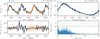 |
Fig. 8 Model combining a long-period planet with a GP model at shorter periods for HIP 64823. Top left: the combined 1P+GP model fitted to the data. Top right: RV residuals after subtracting the GP model, phase-folded to highlight the contribution of the planet. Bottom left: RV residuals after removing the contribution of the planet to highlight the GP model. Bottom right: residual RV periodogram showing only tentative periodicity at shorter periods. The FAPs of 5% (dashed), 1% (dash-dotted), and 0.1% (dotted) are plotted as gray horizontal lines. |
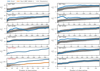 |
Fig. 9 Significance of the amplitude A as a function of the number of observations. The real data are portrayed in blue, while the 1000 realizations of the simulated data are portrayed as gray lines. We evaluated the S-BGLS at the period of the best Keplerian models summarized in Table 3. For the two secure planet hosts, HIP 75458 and HIP 88048 (identifiers marked in red), the simulated relations are plotted on top of the real ones for increased visibility. For HIP 88048, we further plot the significance of the long-period signal in orange. The contributions of the respective other companions were subtracted for the two secure systems. |
7 Discussion
In recent years, a number of intrinsically variable giant stars, some of which had previously been reported to host planets using RV data, have been identified (Hatzes et al. 2018; Delgado Mena et al. 2018, 2023; Reichert et al. 2019; Heeren et al. 2021; Döllinger & Hartmann 2021; Teng et al. 2023b; Zhou et al. 2023; Lee et al. 2023). Given the varying temporal baselines of RV data sets and availability of activity indicators, there could be more false positives among luminous evolved planet hosts. These could have an impact on occurrence rate studies if not treated carefully. Wolthoff et al. (2022), for instance, perform several “homogenizing cuts” to their underlying sample to remove very luminous (log10(L/L⊙) > 3) giants, as well as stars with complex RV signatures. Thus, they reduce the impact false-positive planet detections could have on their conclusions. Despite this careful treatment, the published “planet host” HIP 16335 (Lee et al. 2014) is included as such in their analysis, although we now conclude that its variations are intrinsic.
Within the literature, there is no consensus which process causes these false-positive detections. One candidate could be the rotational modulation of stellar surface features such as hot plages or cool spots. Unfortunately, for most of the stars there are no reliable estimates of the rotation periods due to a lack of photometric variations (see also Table 1). This lack of variations, however, also generally argues against large stellar spots (Reffert et al. 2015; Reichert et al. 2019).
On the other hand, the variations of surface features linked to magnetic activity are yet largely unexplored. As suggested by Delgado Mena et al. (2023, and references therein), magnetic structures on giant stars could locally suppress convection, potentially leading to RV variations without associated photometric variations. This idea seems plausible, given the detection of a weak magnetic surface field of Pollux (Aurière et al. 2009, 2014, 2021), which varies on similar timescales as the RVs. These RV variations have been attributed to an exoplanet companion (Hatzes et al. 2006; Reffert et al. 2006). Recent simulations show that this magnetic field could be dynamo-driven and that the strength of the magnetic field is coupled to the scale of convection cells (Amard et al. 2024). Rolo et al. (2024) discuss a connection between the amplitudes of the activity indicator variations and the Li abundance of the stars. Their work includes the intrinsically variable giants discussed in Delgado Mena et al. (2023), for several of which the Hα index is shown to be periodic close to the RV period. All of these stars are Li-rich, potentially providing another link toward magnetic activity, as high Li abundance is associated with enhanced chromospheric activity (Sneden et al. 2022). Interestingly, strong magnetic fields have also been detected in the cores of some giant stars using Kepler data (Li et al. 2022; Deheuvels et al. 2023; Li et al. 2023). Of the 12 stars in this sample, literature Li abundance measurements are available for eleven. None of them were found to be Li-rich. (Brown et al. 1989; Lèbre et al. 2006; Liu et al. 2014; Charbonnel et al. 2020).
In this context, we find it noteworthy that the chromospheric activity indicators, namely those targeting the Hα, NaD, and CaIRT lines, which are sensitive to magnetic activity (Sarkis et al. 2018), show at least tentative periodic variations at periods similar to the RVs for several of the stars examined in this work. Thus, a connection between magnetic activity and RV variations resembling planets seems plausible. However, further modeling of the RV curves remains challenging lacking a better physical understanding of the magnetic surface fields and convection patterns of giants. It also remains uncertain whether such variations in the chromospheric indicators might also be attributed to other intrinsic mechanisms.
Another promising alternative, long-period non-radial oscillations, was already discussed for giant stars by Hatzes & Cochran (1993). More recently, Hatzes et al. (2018) propose that the RV variations of the luminous giant γ Dra show a beating of different periods that seem to be most elegantly explained by non-radial oscillations. Hatzes et al. (2018) also propose that this new type of variability might be linked to oscillatory convective modes which have been developed by Saio et al. (2015) to explain the so-called sequence D in the period-luminosity plot of bright, variable giants showing long-secondary periods (LSPs) (Wood et al. 1999). Although contested in the literature as the origin of these LSPs (see, for instance, Soszyński & Udalski 2014; Soszyński et al. 2021; Goldberg et al. 2024), Hatzes et al. (2018) and Reichert et al. (2019) argue that γ Dra and Aldebaran occupy a region in a period-luminosity plot that could be crossed by an extrapolation of the models by Saio et al. (2015). This could make oscillatory convective modes a plausible explanation for the RV variations. In Spaeth et al. (2024), we use this idea to show that a simple model of an l = 1, m = 1 non-radial oscillation could explain the RV variations, as well as the correlations with the available activity indicator, for the known false-positive evolved planet host NGC 4349 No. 127 (Delgado Mena et al. 2018, 2023). Although more massive, NGC 4349 No. 127 has a similar luminosity to that of γ Dra and Aldebaran, and shows RV variations of similar period.
Having identified seven additional giant stars with RV variations that resemble planets (at least during part of their temporal baseline) that we regard to be securely of intrinsic origin, we can update Fig. 8 of Reichert et al. (2019) (and Fig. 9 in Spaeth et al. 2024). In Fig. 10, we show luminous and variable giant stars identified in the OGLE-III survey (Soszyński et al. 2009) as small green dots, with the subset of those showing LSPs on sequence D in black. We further plot models of oscillatory convective modes for different stellar masses taken from Saio et al. (2015) in different shades of pink. On top, we present published planet hosts from the Lick survey as red circles, stars that show RV curves resembling planets but have been shown to be of intrinsic origin as blue star markers, and remaining planet candidates, or stars for which we regard the analysis to not yet provide clear conclusions, as cyan hexagons. We highlight the stars examined within this work, marking these with their Hipparcos identifiers, while we show the literature stars with somewhat reduced sizes and lighter shades. We exclude the lower-luminosity false-positive hosts 41 Lyn and 14 And (Teng et al. 2023b) from this analysis. The RV periodicity of both stars closely aligns with a half-yearly cycle, accompanied by a strong yearly signal in the window function. These characteristics suggest that the observed periodicities are more likely related to the observational sampling than to a physical process.
As can be seen, the clear distinction between the secure planet hosts and the false-positive detections highlighted by Reichert et al. (2019) becomes somewhat less striking as more stars are included. While we can still observe a clear trend that the false-positive detections mostly occur for larger luminosities, we can see several such false positives also in the transition region, among these HIP 7607. We note that one of the supposedly confirmed planet hosts in the transition region, HIP 60202 (Liu et al. 2008), was recently challenged by Teng et al. (2023b) due to additional periodicity in the residuals RVs that would be challenging to attribute to an additional companion due to dynamical constraints, akin to the results of the residual analysis in Sect. 4.2 in this work. We also find HIP 16335, whose published planet is likely a misidentified intrinsic signal according to our analysis, to be in close vicinity to other intrinsically variable giants, including γ Dra. The two stars with RV variations of unknown origin at high luminosities, 3 Cnc and 44 UMa (Tala Pinto et al. 2020), have convincing Keplerian models but lack a set of reliable activity indicators other than Lick Hα measurements, which were inconspicuous for these stars. Noteworthy is also the location of HIP 73620, whose RV variations fall within the region occupied by stars who are considered to be secure planet hosts. Although we favor an intrinsic origin of the RV variations, we cannot rule out a planetary companion with certainty. However, assuming our assessment of an intrinsic origin to be correct, this would certainly make the distinction between the groups of the secure hosts and the intrinsically RVvariable stars less clear. However, we also note that HIP 73620 shows the smallest amplitude among the stars in this study.
Finally, we note the locations of HIP 64823 and HIP 89826, which fall far outside the period regime in which the other false positives have been found. In terms of their luminosity they fall into the transition region between the secure planets and the RV-variable stars. At least for HIP 64823, this further supports our interpretation that the RV variations are best explained by a planetary companion. HIP 89826 remains uncertain.
In Fig. 11, we select all stars that are intrinsically RV variable and those of so-far unknown origin from Fig. 10, and plot their semi-amplitude K against their luminosity. We observe that the majority of the stars follows a roughly linear trend with increased K for higher luminosities. We note two strong outliers at high luminosities, which are HIP 46390 and HIP 38253. Especially for the latter, the amplitude in the Lick RVs alone would be somewhat larger than the amplitude derived combining the Lick data with the SONG and CARMENES measurements (see Fig. 2), such that it might also lie at higher K depending on the part of the RV curve that was observed. We emphasize that we also include more likely planet candidates, such as HIP 64823, among the stars of unknown origin.
We further mark the estimated p-mode jitter derived using the scaling relations by Kjeldsen & Bedding (1995) for three different stellar masses in shades of red. These give a rough lower limit of semi-amplitude K that could have been detected. That is, it is possible that the linear trend is merely a consequence of selection effects due to the higher short-term jitter that would likely prevent the detection of longer-period RV variability for more luminous stars. Nevertheless, we find the observed trend noteworthy as it might contribute toward a physical interpretation. A similar trend (expressed in terms of log g, which, however, correlates with L and that can also be observed for our stars) has already been discussed by Hatzes & Cochran (1998).
Overall, we have to conclude that the full picture remains elusive. We can certainly strengthen the finding that planet detections around giant stars with luminosities L ≳ 125 L⊙ should be regarded with caution. We, however, also note the suspicion that HIP 73620, which has much lower luminosity, has intrinsically induced RV variations. While we can somewhat strengthen the suggestions by Hatzes et al. (2018) and Reichert et al. (2019), that an extrapolation of the models of oscillatory convective modes could explain the majority of the false-positive sample, we also find hints of variations in the chromospheric activity indicators for several of the stars, which might suggest a link toward magnetic activity of, perhaps, rather exotic nature. Unlike the case of NGC 4349 No. 127 (Delgado Mena et al. 2018, 2023; Spaeth et al. 2024), we do not find distinctive correlations between the activity indicators and the RVs for any of our stars, which could be easily interpreted as the fingerprints of a single dominating oscillation mode. However, we discuss in Spaeth et al. (2024) that a superposition of different modes along with sizable stellar jitter can hide such correlations. We also note that NGC 4349 No. 127 was also shown to have periodic variations in the Hα indicator (Delgado Mena et al. 2018, 2023), which might suggest that such chromospheric activity could also be linked to oscillations. More detailed investigations, both from the observational and the theoretical sides, are certainly necessary to resolve the mysterious RV variations of luminous evolved stars.
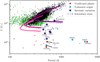 |
Fig. 10 Luminosity of the stars plotted against the RV period. Variable stars from the OGLE survey are plotted in green, with the subset of those showing LSPs on sequence D plotted in black. Overplotted in pink are models from the expected relations of oscillatory convective modes (Saio et al. 2015) for different stellar masses. We plot confirmed planets within the Lick sample as red circles, and confirmed intrinsically RV-variable stars that mimic planets as blue star markers. Stars with as yet undecided origins of their RV variations are shown as cyan hexagons. Stars taken from the literature are shown with reduced marker sizes and lighter shades. We mark the Hipparcos identifiers of the stars discussed in this work. We omit plotting the short-period planet hosts HIP 89587 (Teng et al. 2023a) and HIP 70791 (Takarada et al. 2018) for visual clarity. The plot is adapted from Fig. 8 of Reichert et al. (2019) and Fig. 9 of Spaeth et al. (2024). |
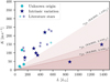 |
Fig. 11 Semi-amplitude K of the intrinsically RV-variable stars (blue star markers) and the stars with as yet unknown origin of their RV variations (cyan hexagons) plotted against the luminosity. The literature stars are plotted with reduced sizes. We further plot the estimated p-mode jitter following the scaling relations by Kjeldsen & Bedding (1995), labeled K&B95, for three different stellar masses. We observe that many of the stars follow a roughly linear relation between the amplitude of their RV variation and the luminosity. Two outliers at large L but small K are noted. These are HIP 46390 and HIP 38253. We exclude the very luminous star NGC 2345 No. 50 from the plot for visual clarity. |
8 Summary
The goal of this study was to test ten bright evolved stars identified as planet candidates after the conclusion of the 12-year Lick RV survey for the presence of planets using the SONG and CARMENES spectrographs. We further aimed to assess the effectiveness of different standard metrics used in the literature to differentiate between planets and intrinsic variations when applied to giant stars. Finally, we were motivated to also highlight the false-positive detections in order to provide new evidence of the observational fingerprints of the mysterious RV variations of luminous giant stars.
We find that seven out of the ten former planet candidate stars have an intrinsic origin of their RV variations. These are HIP 7607, HIP 7884, HIP 38253, HIP 46390, HIP 47959, HIP 84671, and (most notably) HIP 16335. Significantly, HIP 16335 was previously reported by Lee et al. (2014) to host a 6.5 MJup minimum mass giant exoplanet in a 579.8 d orbit, which we reveal to be a misidentified intrinsic RV signal. Furthermore, we lean toward an intrinsic origin for the (comparably) low-amplitude RV variations of HIP 73620, whereas we cannot draw reliable conclusions for HIP 89826. Finally, we find that HIP 64823 remains a promising candidate to host a long-period planet (P ∼  d), and we showed that a GP model can be used to explain residual variability at shorter periodicity. However, as the baseline of the CARMENES observations is not yet long enough, we cannot confirm the presence of the exoplanet candidate with minimum mass mp sin (i) =
  MJup with certainty.
Although the RV variations of most of the intrinsically variable giants are convincingly not caused by exoplanet companions, we find that testing the consistency of the RV amplitude between the optical and the infrared is not effective enough to rule out the possibility that the giants are being orbited by planets given the large stellar jitter. We further find that testing for linear correlations between the activity indicators and the RVs does not detect the majority of the false-positive planet hosts and thus caution relying solely on such metrics. We instead find that for the most luminous stars, clear changes of the dominating periodicity on timescales of tens of years can be observed. A similar effect is also apparent from analyzing the residual RVs, which often show significant remaining periodicity close to the proposed orbital period, which we interpret as the consequences of changing periods or amplitudes. We also observed that testing the consistency of the best Keplerian model with the real data, based on the significance of the amplitude derived from stacked Bayesian GLS periodograms, reliably picks out the false-positive hosts. For such tests, long-term RV monitoring is critical.
Generally, we find that analyzing the CARMENES activity indicators using maximum likelihood periodograms as well as a DBSCAN cluster analysis can, in most cases, detect the intrinsic variability. However, a detailed analysis combining the findings from different indicators is necessary to rule out planetary companions with certainty, as the signals in the activity indicators are typically not very strong, meaning that they can be easily missed. We also observed that even for the well-studied exoplanet host HIP 75458, there are hints in the activity indicators and RV residuals that suggest the current metrics may not be entirely robust at differentiating between planetary and stellar activity signals.
Finally, we discuss the additional detection of intrinsically RV-variable giant stars mimicking exoplanets in the context of other false-positive evolved planet hosts. We find that the general trend that most false positives have high luminosities holds up, but we also found one suspicious case at lower luminosity. We observed a slight trend of increasing RV amplitudes with increasing luminosity. Given the high luminosities of the majority of the stars, a connection to oscillatory convective modes (Saio et al. 2015) seems plausible. However, we do not find any clear correlations between the activity indicators and the RVs in this sample, which would allow for a more detailed assessment of potential oscillation modes (Spaeth et al. 2024). We also note that for several of the stars in the sample and in the literature, chromospheric activity indicators contribute to refuting the planetary companions. These might suggest a connection to magnetic or convective processes in these giants. The phenomenon as a whole remains poorly understood.
With this work, we hope to contribute to a better physical understanding of RV variations of luminous giant stars, which convincingly mimic exoplanet companions. Future research both from the observational and theoretical side are certainly necessary to ultimately resolve the mystery.
Data availability
RVs and activity indicator measurements are available at the CDS via anonymous ftp to cdsarc.cds.unistra.fr (130.79.128.5) or via https://cdsarc.cds.unistra.fr/viz-bin/cat/J/A+A/697/A32
Acknowledgements
We thank the anonymous referee for their valuable feedback, which helped improve the quality of this work. This work was supported by the Deutsche Forschungsgemeinschaft (DFG) within the Priority Program SPP 1992 “The Diversity of Exoplanets” (RE 2694/7-1). T.T. acknowledges support by the BNSF program “VIHREN-2021” project No. KP-06-DV/5. We would like to thank the staff at Lick observatory for their support and thank the CAT observers who assisted with this project, including David Mitchell, Saskia Hekker, Christian Schwab, Christoph Bergmann, Kirsten Vincke, Julian Stürmer, Kelsey Clubb, David Bauer, Dominika Wylezalek, Dennis Kügler, and Debra Fischer. This work is based on observations made with the Hertzsprung SONG telescope operated on the Spanish Observatorio del Teide on the island of Tenerife by the Aarhus and Copenhagen Universities and by the Instituto de Astrofísica de Canarias. It is further based on observations collected at the Centro Astronómico Hispano en Andalucía (CAHA) at Calar Alto, proposals F16-3.5-024, H17-3.5-014, F18-3.5-016, H18-3.5-015, 21A-3.5-051, 21B-3.5-052, 22A-3.5-051, 22B-3.5-051, 23A-3.5-051, 23B-3.5-052, operated jointly by Junta de Andalucía and Consejo Superior de Investigaciones Científicas (IAA-CSIC). Based on data from the CAHA Archive at CAB (INTA-CSIC)9. The CAHA Archive is part of the Spanish Virtual Observatory10 project funded by MCIN/AEI/10.13039/501100011033 through grant PID2020-112949GB-I00. This project has received funding from the European Union’s Horizon 2020 research and innovation programme under grant agreement No 101004719. This research has made use of the VizieR catalog access tool and the SIMBAD database, operated at CDS, Strasbourg, France. This work has made use of data from the European Space Agency (ESA) mission Gaia (https://www.cosmos.esa.int/gaia), processed by the Gaia Data Processing and Analysis Consortium (DPAC, https://www.cosmos.esa.int/web/gaia/dpac/consortium). Funding for the DPAC has been provided by national institutions, in particular the institutions participating in the Gaia Multilateral Agreement. This research made use of Astropy11, a community-developed core Python package for Astronomy. We further acknowledge use of the python packages NumPy (Harris et al. 2020), SciPy (Virtanen et al. 2020), Matplotlib (Hunter 2007), seaborn (Waskom 2021), pandas (The pandas development team 2024; McKinney 2010), PyAstronomy12 (Czesla et al. 2019), lmfit (Newville et al. 2021), DYNESTY (Speagle 2020), celerite (Foreman-Mackey et al. 2017), corner (Foreman-Mackey 2016), scikit-learn (Pedregosa et al. 2011), bgls (Mortier et al. 2015), astroquery (Ginsburg et al. 2019), dill (McKerns et al. 2012), and the RV fitting tool Exo-Striker (Trifonov 2019).
Appendix A Results of the activity periodogram analysis
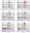 |
Fig. A.1 Maximum likelihood periodograms for six sample stars. The top panel for each star portrays the combined RV MLP. In the remaining panels, we show the MLPs of the RVs (black) and activity indicators (see legend) for each instrument. The FAPs of 5% (dashed), 1% (dash-dotted), and 0.1% (dotted) are plotted as gray horizontal lines. The bottom panel shows the instruments’ window functions derived as discrete Fourier transforms. The thick, red, vertical line indicates the period of the Keplerian fit (see Table 3). The alias periods, corresponding to the most significant peak in the respective window function, are shown as thinner lines. The positions of these window peaks are marked with colored arrows in the bottom panels. Notably, the CARMENES VIS and NIR window functions largely overlap. Additionally, we display the harmonics and sub-harmonics of the period of the Keplerian fit as red lines with lower opacity. |
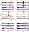 |
Fig. A.2 Maximum likelihood periodograms for the remaining six stars. The same description as in Fig. A.1 applies. The FAPs of 5% (dashed), 1% (dash-dotted), and 0.1% (dotted) are plotted as gray horizontal lines. The identifiers of the two planet hosts, HIP 75458 and HIP 88048, are marked in red. For HIP 80488, we mark the second significant periodicity, corresponding to the outer brown-dwarf companion, as the violet, vertical line. We omit plotting its aliases and harmonics for visual clarity. |
Appendix B Results of the DBSCAN clustering algorithm
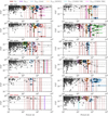 |
Fig. B.1 Results of the DBSCAN clustering algorithm. In each panel, all identified peaks in the MLPs of the CARMENES activity indicators are shown as filled circles. Arbitrarily colored circles represent activity peaks assigned to clusters by DBSCAN, while gray circles indicate peaks that are not part of any cluster. The larger, empty circles indicate the center periods and FAPs of the clusters. We further overplot the FAP levels of 5% (dashed), 1% (dash-dotted), and 0.1% (dotted) as horizontal gray lines, and the fitted RV period (thick), its aliases (thin, based on the VIS window function), and harmonics (lower opacity) as vertical red lines. Furthermore, for stars where individual instruments exhibit a strongest period that deviates from the fitted period by at least 10% (restricted to 100 d < Pmax < 5000 d), we overplot the strongest RV period detected in the MLP of the respective instrument using vertical, colored lines specified in the figure legend. The identifiers of the two planet hosts, HIP 75458 and HIP 88048, are marked in red. For the latter, we also mark the periodicity of the outer orbital companion in violet. |
Appendix C Priors used for the Keplerian modeling
Appendix D Corner plot of the joint 1P+GP model for HIP 64823
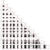 |
Fig. D.1 Corner plot of the posterior samples of the joint 1P+GP model for HIP 64283. The mode of each parameter, marked as the continuous, red line, was adopted as the best fitting parameter in Table 4. The red dashed lines mark the interval that contains 68% of the posterior samples. We note that the posteriors of the planet model are well constrained, while the posteriors of the GP model (especially the factor C) are relatively broad and thus allow for a wide range of models. |
References
- Alves, D. R., 2000, ApJ, 539, 732 [NASA ADS] [CrossRef] [Google Scholar]
- Amard, L., Brun, A. S., & Palacios, A., 2024, ApJ, 974, 311 [Google Scholar]
- Andersen, M. F., Grundahl, F., Christensen-Dalsgaard, J., et al. 2014, in Rev. Mex. Astron. Astrofis. Conf. Ser., 45, 83 [Google Scholar]
- Assef, R. J., Gaudi, B. S., & Stanek, K. Z., 2009, ApJ, 701, 1616 [NASA ADS] [CrossRef] [Google Scholar]
- Aurière, M., Wade, G. A., Konstantinova-Antova, R., et al. 2009, A&A, 504, 231 [NASA ADS] [CrossRef] [EDP Sciences] [Google Scholar]
- Aurière, M., Konstantinova-Antova, R., Espagnet, O., et al. 2014, Magnetic Fields throughout Stellar Evolution, eds. P. Petit, M. Jardine, & H. C. Spruit, IAU Symposium, 302, 359 [Google Scholar]
- Aurière, M., Petit, P., Mathias, P., et al. 2021, A&A, 646, A130 [EDP Sciences] [Google Scholar]
- Boisse, I., Moutou, C., Vidal-Madjar, A., et al. 2009, A&A, 495, 959 [NASA ADS] [CrossRef] [EDP Sciences] [Google Scholar]
- Bressan, A., Marigo, P., Girardi, Léo.,, et al. 2012, MNRAS, 427, 127 [NASA ADS] [CrossRef] [Google Scholar]
- Brown, J. A., Sneden, C., Lambert, D. L., & Dutchover, Jr., E. 1989, ApJS, 71, 293 [NASA ADS] [CrossRef] [Google Scholar]
- Burt, J. A., Hooton, M. J., Mamajek, E. E., et al. 2024, ApJ, 971, L12 [NASA ADS] [CrossRef] [Google Scholar]
- Butler, R. P., Marcy, G. W., Williams, E., et al. 1996, PASP, 108, 500 [Google Scholar]
- Campante, T. L., Li, T., Ong, J. M. J., et al. 2023, AJ, 165, 214 [NASA ADS] [CrossRef] [Google Scholar]
- Charbonnel, C., Lagarde, N., Jasniewicz, G., et al. 2020, A&A, 633, A34 [NASA ADS] [CrossRef] [EDP Sciences] [Google Scholar]
- Cox, J. P., King, D. S., & Stellingwerf, R. F., 1972, ApJ, 171, 93 [NASA ADS] [CrossRef] [Google Scholar]
- Czesla, S., Molle, T., & Schmitt, J. H. M. M., 2018, A&A, 609, A39 [NASA ADS] [CrossRef] [EDP Sciences] [Google Scholar]
- Czesla, S., Schröter, S., Schneider, C. P., et al. 2019, Astrophysics Source Code Library [record ascl:1906.010] [Google Scholar]
- Dalal, S., Rescigno, F., Cretignier, M., et al. 2024, MNRAS, 531, 4464 [Google Scholar]
- Deheuvels, S., Li, G., Ballot, J., & Lignières, F., 2023, A&A, 670, L16 [NASA ADS] [CrossRef] [EDP Sciences] [Google Scholar]
- Delgado Mena, E., Lovis, C., Santos, N. C., et al. 2018, A&A, 619, A2 [NASA ADS] [CrossRef] [EDP Sciences] [Google Scholar]
- Delgado Mena, E., Gomes da Silva, J., Faria, J. P.,, et al. 2023, A&A, 679, A94 [NASA ADS] [CrossRef] [EDP Sciences] [Google Scholar]
- Desort, M., Lagrange, A. M., Galland, F., Udry, S., & Mayor, M., 2007, A&A, 473, 983 [CrossRef] [EDP Sciences] [Google Scholar]
- Díaz, R. F., Cincunegui, C., & Mauas, P. J. D., 2007, MNRAS, 378, 1007 [Google Scholar]
- Döllinger, M. P., & Hartmann, M., 2021, ApJS, 256, 10 [CrossRef] [Google Scholar]
- Dreizler, S., Luque, R., Ribas, I., et al. 2024, A&A, 684, A117 [NASA ADS] [CrossRef] [EDP Sciences] [Google Scholar]
- Ernst, M. D., 2004, Stat. Sci., 19, 676 [Google Scholar]
- ESA 1997, ESA Spec. Publ., 1200 [Google Scholar]
- Ester, M., Kriegel, H.-P., Sander, J., & Xu, X., 1996, in Proc. 2nd Int. Conf. Knowl. Discov, 226 [Google Scholar]
- Feroz, F., Hobson, M. P., & Bridges, M., 2009, MNRAS, 398, 1601 [NASA ADS] [CrossRef] [Google Scholar]
- Fischer, D. A., & Valenti, J., 2005, ApJ, 622, 1102 [NASA ADS] [CrossRef] [Google Scholar]
- Fischer, D. A., Marcy, G. W., & Spronck, J. F. P., 2013, ApJS, 210, 5 [NASA ADS] [CrossRef] [Google Scholar]
- Foreman-Mackey, D., 2016, J. Open Source Softw., 1, 24 [Google Scholar]
- Foreman-Mackey, D., Agol, E., Ambikasaran, S., & Angus, R., 2017, AJ, 154, 220 [Google Scholar]
- Fredslund Andersen, M., Handberg, R., Weiss, E., et al. 2019, PASP, 131, 045003 [Google Scholar]
- Frink, S., Quirrenbach, A., Fischer, D., Röser, S., & Schilbach, E., 2001, PASP, 113, 173 [Google Scholar]
- Frink, S., Mitchell, D. S., Quirrenbach, A., Fischer, D. A., & Marcy, G. W., 2002, ApJ, 576, 7 [Google Scholar]
- Gaia Collaboration (Prusti, T., et al.,) 2016, A&A, 595, A1 [NASA ADS] [CrossRef] [EDP Sciences] [Google Scholar]
- Gaia Collaboration (Vallenari, A., et al.,) 2023, A&A, 674, A1 [NASA ADS] [CrossRef] [EDP Sciences] [Google Scholar]
- Galland, F., Lagrange, A.-M., Udry, S., et al. 2005, A&A, 443, 337 [NASA ADS] [CrossRef] [EDP Sciences] [Google Scholar]
- Gehan, C., Godoy-Rivera, D., & Gaulme, P., 2024, A&A, 686, A93 [NASA ADS] [CrossRef] [EDP Sciences] [Google Scholar]
- Ginsburg, A., Sipőcz, B. M., Brasseur, C. E., et al. 2019, AJ, 157, 98 [Google Scholar]
- Goldberg, J. A., Joyce, M., & Molnár, L., 2024, ApJ, 977, 35 [Google Scholar]
- Golovin, A., Reffert, S., Just, A., et al. 2023, A&A, 670, A19 [NASA ADS] [CrossRef] [EDP Sciences] [Google Scholar]
- Grundahl, F., Andersen, M. F., Christensen-Dalsgaard, J., et al. 2017, ApJ, 836, 142 [Google Scholar]
- Harris, C. R., Millman, K. J., van der Walt, S. J., et al. 2020, Nature, 585, 357 [NASA ADS] [CrossRef] [Google Scholar]
- Hatzes, A. P., 1996, PASP, 108, 839 [NASA ADS] [CrossRef] [Google Scholar]
- Hatzes, A. P., 2013, Astron. Nachr., 334, 616 [NASA ADS] [CrossRef] [Google Scholar]
- Hatzes, A. P., & Cochran, W. D., 1993, ApJ, 413, 339 [CrossRef] [Google Scholar]
- Hatzes, A. P., & Cochran, W. D., 1994, ApJ, 422, 366 [NASA ADS] [CrossRef] [Google Scholar]
- Hatzes, A. P., & Cochran, W. D., 1998, in ASP Conf. Ser., 154, 311 [Google Scholar]
- Hatzes, A. P., Cochran, W. D., Endl, M., et al. 2006, A&A, 457, 335 [NASA ADS] [CrossRef] [EDP Sciences] [Google Scholar]
- Hatzes, A. P., Endl, M., Cochran, W. D., et al. 2018, AJ, 155, 120 [NASA ADS] [CrossRef] [Google Scholar]
- Heeren, P., Reffert, S., Trifonov, T., et al. 2021, A&A, 647, A160 [NASA ADS] [CrossRef] [EDP Sciences] [Google Scholar]
- Heeren, P., Tronsgaard, R., Grundahl, F., et al. 2023, A&A, 674, A164 [NASA ADS] [CrossRef] [EDP Sciences] [Google Scholar]
- Hekker, S., & Meléndez, J., 2007, A&A, 475, 1003 [NASA ADS] [CrossRef] [EDP Sciences] [Google Scholar]
- Hekker, S., Reffert, S., & Quirrenbach, A., 2005, arXiv e-prints [arXiv:astro-ph/0510337] [Google Scholar]
- Hekker, S., Reffert, S., Quirrenbach, A., et al. 2006, A&A, 454, 943 [NASA ADS] [CrossRef] [EDP Sciences] [Google Scholar]
- Hekker, S., Snellen, I. A. G., Aerts, C., et al. 2008, A&A, 480, 215 [NASA ADS] [CrossRef] [EDP Sciences] [Google Scholar]
- Higson, E., Handley, W., Hobson, M., & Lasenby, A., 2019, Stat. Comput., 29, 891 [Google Scholar]
- Hill, M. L., Kane, S. R., Campante, T. L., et al. 2021, AJ, 162, 211 [NASA ADS] [CrossRef] [Google Scholar]
- Huang, X., He, Y., Bai, Z., et al. 2024, ApJS, 272, 6 [NASA ADS] [CrossRef] [Google Scholar]
- Huélamo, N., Figueira, P., Bonfils, X., et al. 2008, A&A, 489, L9 [NASA ADS] [CrossRef] [EDP Sciences] [Google Scholar]
- Hunter, J. D., 2007, Comput. Sci. Eng., 9, 90 [NASA ADS] [CrossRef] [Google Scholar]
- Johnson, J. A., Fischer, D. A., Marcy, G. W., et al. 2007, ApJ, 665, 785 [Google Scholar]
- Kane, S. R., Reffert, S., Henry, G. W., et al. 2010, ApJ, 720, 1644 [Google Scholar]
- Kemmer, J., Lafarga, M., Fuhrmeister, B., et al. 2025, A&A, in press, https://doi.org/10.1051/0004-6361/202347056 [NASA ADS] [CrossRef] [EDP Sciences] [Google Scholar]
- Kjeldsen, H., & Bedding, T. R., 1995, A&A, 293, 87 [NASA ADS] [Google Scholar]
- Kjeldsen, H., & Bedding, T. R., 2011, A&A, 529, L8 [NASA ADS] [CrossRef] [EDP Sciences] [Google Scholar]
- Koposov, S., Speagle, J., Barbary, K., et al. 2024, https://doi.org/10.5281/zenodo.12537467 [Google Scholar]
- Kürster, M., Endl, M., Rouesnel, F., et al. 2003, A&A, 403, 1077 [NASA ADS] [CrossRef] [EDP Sciences] [Google Scholar]
- Lafarga, M., Ribas, I., Lovis, C., et al. 2020, A&A, 636, A36 [NASA ADS] [CrossRef] [EDP Sciences] [Google Scholar]
- Lagrange, A.-M., Desort, M., Galland, F., Udry, S., & Mayor, M., 2009, A&A, 495, 335 [NASA ADS] [CrossRef] [EDP Sciences] [Google Scholar]
- Laney, C. D., Joner, M. D., & Pietrzyński, G., 2012, MNRAS, 419, 1637 [Google Scholar]
- Lèbre, A., de Laverny, P., Do Nascimento, Jr., J. D., & de Medeiros, J. R. 2006, A&A, 450, 1173 [NASA ADS] [CrossRef] [EDP Sciences] [Google Scholar]
- Lee, B.-C., Han, I., Park, M.-G., et al. 2014, J. Korean Astron. Soc., 47, 69 [NASA ADS] [CrossRef] [Google Scholar]
- Lee, B.-C., Koo, J.-R., Choi, Y.-H., et al. 2023, J. Korean Astron. Soc., 56, 277 [Google Scholar]
- Li, G., Deheuvels, S., Ballot, J., & Lignières, F., 2022, Nature, 610, 43 [NASA ADS] [CrossRef] [Google Scholar]
- Li, G., Deheuvels, S., Li, T., Ballot, J., & Lignières, F., 2023, A&A, 680, A26 [NASA ADS] [CrossRef] [EDP Sciences] [Google Scholar]
- Liu, Y. J., Sato, B., Zhao, G., et al. 2008, ApJ, 672, 553 [NASA ADS] [CrossRef] [Google Scholar]
- Liu, Y. J., Tan, K. F., Wang, L., et al. 2014, ApJ, 785, 94 [NASA ADS] [CrossRef] [Google Scholar]
- Lovis, C., & Mayor, M., 2007, A&A, 472, 657 [NASA ADS] [CrossRef] [EDP Sciences] [Google Scholar]
- Luque, R., Trifonov, T., Reffert, S., et al. 2019, A&A, 631, A136 [NASA ADS] [CrossRef] [EDP Sciences] [Google Scholar]
- Malla, S. P., Stello, D., Montet, B. T., et al. 2024, MNRAS, 534, 1775 [Google Scholar]
- Martin, J., Fuhrmeister, B., Mittag, M., et al. 2017, A&A, 605, A113 [NASA ADS] [CrossRef] [EDP Sciences] [Google Scholar]
- Martínez-Arnáiz, R., López-Santiago, J., Crespo-Chacón, I., & Montes, D., 2011, MNRAS, 414, 2629 [CrossRef] [Google Scholar]
- Mayor, M., Pepe, F., Queloz, D., et al. 2003, The Messenger, 114, 20 [NASA ADS] [Google Scholar]
- McKerns, M. M., Strand, L., Sullivan, T., Fang, A., & Aivazis, M. A. G., 2012, arXiv e-prints [arXiv:1202.1056] [Google Scholar]
- McKinney, W., 2010, in Proc. 9th Python Sci. Conf., eds. S. van der Walt, & Jarrod Millman, 56 [CrossRef] [Google Scholar]
- Mitchell, D. S., Reffert, S., Trifonov, T., Quirrenbach, A., & Fischer, D. A., 2013, A&A, 555, A87 [NASA ADS] [CrossRef] [EDP Sciences] [Google Scholar]
- Mortier, A., & Collier Cameron, A., 2017, A&A, 601, A110 [NASA ADS] [CrossRef] [EDP Sciences] [Google Scholar]
- Mortier, A., Faria, J. P., Correia, C. M., Santerne, A., & Santos, N. C., 2015, A&A, 573, A101 [NASA ADS] [CrossRef] [EDP Sciences] [Google Scholar]
- Müller, R. G., 2019, Bachelor’s thesis, University of Heidelberg, Germany [Google Scholar]
- Nagel, E., Czesla, S., Kaminski, A., et al. 2023, A&A, 680, A73 [NASA ADS] [CrossRef] [EDP Sciences] [Google Scholar]
- Newville, M., Otten, R., Nelson, A., et al. 2021, https://doi.org/10.5281/zenodo.5570790 [Google Scholar]
- Ortiz, M., Reffert, S., Trifonov, T., et al. 2016, A&A, 595, A55 [NASA ADS] [CrossRef] [EDP Sciences] [Google Scholar]
- Pedregosa, F., Varoquaux, G., Gramfort, A., et al. 2011, J. Mach. Learn. Res., 12, 2825 [Google Scholar]
- Percy, J. R., Wilson, J. B., & Henry, G. W., 2001, PASP, 113, 983 [CrossRef] [Google Scholar]
- Phipson, B., & Smyth, G. K., 2010, Stat. Appl. Genet. Mol. Biol., 9, 39 [Google Scholar]
- Quirrenbach, A., Reffert, S., & Bergmann, C., 2011, AIP Conf. Ser., 1331, 102 [Google Scholar]
- Quirrenbach, A., Amado, P. J., Caballero, J. A., et al. 2014, SPIE Conf. Ser., 9147, 91471F [Google Scholar]
- Quirrenbach, A., Trifonov, T., Lee, M. H., & Reffert, S., 2019, A&A, 624, A18 [NASA ADS] [CrossRef] [EDP Sciences] [Google Scholar]
- Reffert, S., Quirrenbach, A., Mitchell, D. S., et al. 2006, ApJ, 652, 661 [NASA ADS] [CrossRef] [Google Scholar]
- Reffert, S., Bergmann, C., Quirrenbach, A., Trifonov, T., & Künstler, A., 2015, A&A, 574, A116 [NASA ADS] [CrossRef] [EDP Sciences] [Google Scholar]
- Reichert, K., Reffert, S., Stock, S., Trifonov, T., & Quirrenbach, A., 2019, A&A, 625, A22 [NASA ADS] [CrossRef] [EDP Sciences] [Google Scholar]
- Reiners, A., Bean, J. L., Huber, K. F., et al. 2010, ApJ, 710, 432 [Google Scholar]
- Reiners, A., Zechmeister, M., Caballero, J. A., et al. 2018, A&A, 612, A49 [NASA ADS] [CrossRef] [EDP Sciences] [Google Scholar]
- Ribas, I., Reiners, A., Zechmeister, M., et al. 2023, A&A, 670, A139 [NASA ADS] [CrossRef] [EDP Sciences] [Google Scholar]
- Robertson, P., Mahadevan, S., Endl, M., & Roy, A., 2014, Science, 345, 440 [Google Scholar]
- Rolo, I., Delgado Mena, E., Tsantaki, M., & Gomes da Silva, J. 2024, A&A, 688, A68 [NASA ADS] [CrossRef] [EDP Sciences] [Google Scholar]
- Saio, H., Wood, P. R., Takayama, M., & Ita, Y., 2015, MNRAS, 452, 3863 [Google Scholar]
- Sarkis, P., Henning, T., Kürster, M., et al. 2018, AJ, 155, 257 [NASA ADS] [CrossRef] [Google Scholar]
- Sato, B., Ando, H., Kambe, E., et al. 2003, ApJ, 597, L157 [Google Scholar]
- Sato, B., Izumiura, H., Toyota, E., et al. 2007, ApJ, 661, 527 [NASA ADS] [CrossRef] [Google Scholar]
- Schäfer, S., Guenther, E. W., Reiners, A., et al. 2018, SPIE Conf. Ser., 10702, 1070276 [Google Scholar]
- Schöfer, P., Jeffers, S. V., Reiners, A., et al. 2019, A&A, 623, A44 [Google Scholar]
- Schwab, C., 2010, PhD thesis, University of Heidelberg, Germany [Google Scholar]
- Skilling, J., 2004, in AIP Conf. Ser., 735, Bayesian Inference and Maximum Entropy Methods in Science and Engineering: 24th International Workshop on Bayesian Inference and Maximum Entropy Methods in Science and Engineering, eds. R. Fischer, R. Preuss, & U. V. Toussaint (AIP), 395 [Google Scholar]
- Skilling, J., 2006, Bayesian Anal., 1, 833 [Google Scholar]
- Sneden, C., Afşar, M., Bozkurt, Z., et al. 2022, ApJ, 940, 12 [NASA ADS] [CrossRef] [Google Scholar]
- Soszyński, I., & Udalski, A., 2014, ApJ, 788, 13 [Google Scholar]
- Soszyński, I., Udalski, A., Szymański, M. K., et al. 2009, Acta Astron., 59, 239 [Google Scholar]
- Soszyński, I., Olechowska, A., Ratajczak, M., et al. 2021, ApJ, 911, L22 [CrossRef] [Google Scholar]
- Spaeth, D., Reffert, S., Hunt, E. L., Kaminski, A., & Quirrenbach, A., 2024, A&A, 689, A91 [NASA ADS] [CrossRef] [EDP Sciences] [Google Scholar]
- Speagle, J. S., 2020, MNRAS, 493, 3132 [Google Scholar]
- Staudt, P., 2020, Bachelor’s thesis, University of Heidelberg, Germany [Google Scholar]
- Stock, S., Reffert, S., & Quirrenbach, A., 2018, A&A, 616, A33 [NASA ADS] [CrossRef] [EDP Sciences] [Google Scholar]
- Stock, S., Kemmer, J., Kossakowski, D., et al. 2023, A&A, 674, A108 [NASA ADS] [CrossRef] [EDP Sciences] [Google Scholar]
- Stoehr, F., White, R., Smith, M., et al. 2008, in Astronomical Society of the Pacific Conference Series, 394, Astron. Data Anal. Softw. Syst. XVII, eds. R. W. Argyle, P. S. Bunclark, & J. R. Lewis, 505 [Google Scholar]
- Takarada, T., Sato, B., Omiya, M., et al. 2018, PASJ, 70, 59 [NASA ADS] [CrossRef] [Google Scholar]
- Tala, M., Heeren, P., Grill, M., et al. 2016, SPIE Conf. Ser., 9908, 990860 [NASA ADS] [Google Scholar]
- Tala Pinto, M., Reffert, S., Quirrenbach, A., et al. 2020, A&A, 644, A1 [NASA ADS] [CrossRef] [EDP Sciences] [Google Scholar]
- Teng, H.-Y., Sato, B., Kunitomo, M., et al. 2023a, PASJ, 75, 169 [Google Scholar]
- Teng, H.-Y., Sato, B., Kuzuhara, M., et al. 2023b, PASJ, 75, 1030 [NASA ADS] [CrossRef] [Google Scholar]
- The pandas development team 2024, https://doi.org/10.5281/zenodo.10537285 [Google Scholar]
- Trifonov, T., 2019, The Exo-Striker: Transit and Radial Velocity Interactive Fitting Tool for Orbital Analysis and N-body Simulations, Astrophysics Source Code Library [record ascl:1906.004] [Google Scholar]
- Trifonov, T., Reffert, S., Tan, X., Lee, M. H., & Quirrenbach, A., 2014, A&A, 568, A64 [NASA ADS] [CrossRef] [EDP Sciences] [Google Scholar]
- Trifonov, T., Reffert, S., Zechmeister, M., Reiners, A., & Quirrenbach, A., 2015, A&A, 582, A54 [NASA ADS] [CrossRef] [EDP Sciences] [Google Scholar]
- Trotta, R., 2008, Contemp. Phys., 49, 71 [Google Scholar]
- Udry, S., & Santos, N. C., 2007, ARAA, 45, 397 [Google Scholar]
- VanderPlas, J. T., 2018, ApJS, 236, 16 [Google Scholar]
- Virtanen, P., Gommers, R., Oliphant, T. E., et al. 2020, Nat. Methods, 17, 261 [Google Scholar]
- Vogt, S. S., 1987, PASP, 99, 1214 [NASA ADS] [CrossRef] [Google Scholar]
- Von Stauffenberg, A., Trifonov, T., Quirrenbach, A., et al. 2024, A&A, 688, A112 [NASA ADS] [CrossRef] [EDP Sciences] [Google Scholar]
- Waskom, M. L., 2021, J. Open Source Softw., 6, 3021 [CrossRef] [Google Scholar]
- Wittenmyer, R. A., Endl, M., Wang, L., et al. 2011, ApJ, 743, 184 [NASA ADS] [CrossRef] [Google Scholar]
- Wolthoff, V., Reffert, S., Quirrenbach, A., et al. 2022, A&A, 661, A63 [NASA ADS] [CrossRef] [EDP Sciences] [Google Scholar]
- Wood, P. R., Alcock, C., Allsman, R. A., et al. 1999, in Asymptot. Giant Branch Stars, 191, eds. T. Le Bertre, A. Lebre, & C. Waelkens, 151 [Google Scholar]
- Zaire, B., Donati, J. F., Alencar, S. P., et al. 2024, MNRAS, 533, 2893 [Google Scholar]
- Zechmeister, M., & Kürster, M., 2009, A&A, 496, 577 [CrossRef] [EDP Sciences] [Google Scholar]
- Zechmeister, M., Reffert, S., Hatzes, A. P., Endl, M., & Quirrenbach, A., 2008, A&A, 491, 531 [NASA ADS] [CrossRef] [EDP Sciences] [Google Scholar]
- Zechmeister, M., Reiners, A., Amado, P. J., et al. 2018, A&A, 609, A12 [NASA ADS] [CrossRef] [EDP Sciences] [Google Scholar]
- Zechmeister, M., Dreizler, S., Ribas, I., et al. 2019, A&A, 627, A49 [NASA ADS] [EDP Sciences] [Google Scholar]
- Zhou, Q., Latham, D. W., Quinn, S. N., et al. 2023, AJ, 166, 160 [NASA ADS] [CrossRef] [Google Scholar]
All Tables
Number of spectra collected per instrument along with the observational time baselines (years in parentheses).
All Figures
|
Fig. 1 Color-magnitude diagram based on Gaia DR3 photometry showing the location of the sample stars using blue star markers as well as red diamonds for the two published planet hosting giants ι Dra and ν Oph. We also plot the location of the remaining 361 giant stars within the Lick sample in purple. For comparison, we overplot the fifth catalog of nearby stars (CNS5) (Golovin et al. 2023) in dark blue and three adjacent evolutionary tracks for 1 M⊙ (green), 2 M⊙ (black), and 3 M⊙ (purple) taken from PARSEC (Bressan et al. 2012). |
| In the text | |
|
Fig. 2 Best Keplerian models for the 12 stars in the sample. The error bars of the RVs, representing the formal uncertainties of the measurements, are typically smaller than the markers. The identifiers of the two planet hosts, HIP 75458 and HIP 88048, are marked in red. Significant intrinsic RV jitter is present for most of the stars. |
| In the text | |
|
Fig. 3 Maximum likelihood periodograms of the RVs (left) and the residuals (right) after subtracting the best Keplerian model. As the SONG RVs are known to show spurious RV periodicity at a one-year period (Heeren et al. 2023), we plot the MLPs of the residual RVs excluding the SONG data in blue, while the periodograms including the SONG data are shown in orange. The FAPs of 5% (dashed), 1% (dash-dotted), and 0.1% (dotted) are plotted as gray horizontal lines. The identifiers of the two planet hosts, HIP 75458 and HIP 88048, are marked in red. Significant periodicity remains close to the strongest RV period after removing the best fit for many of the stars. |
| In the text | |
|
Fig. 4 Semi-amplitudes K from the CARMENES-NIR channel plotted against the semi-amplitudes in the VIS channel. We highlight the two secure planet hosts, ι Dra and ν Oph as red diamonds, while we show the planet candidates in blue. For ι Dra and ν Oph, only the inner orbital components are examined due to the short baseline of the CARMENES observations. |
| In the text | |
|
Fig. 5 Results of the linear correlation analysis. For each star we show the significance of the linear correlation between the activity indicator labeled on the x-axis and the respective RV data set. Red colors indicate significant (p < 0.1%) linear correlations, while orange colors represent tentative (0.1% ≤ p < 5%) correlations. The identifiers of the two planet hosts, HIP 75458 and HIP 88048, are marked in red. |
| In the text | |
|
Fig. 6 Maximum likelihood periodograms for two example stars. The top panel for each star portrays the combined RV MLP. In the remaining panels, we show the MLPs of the RVs (black) and activity indicators (see legend) for each instrument. The FAPs of 5% (dashed), 1% (dash-dotted), and 0.1% (dotted) are plotted as gray horizontal lines. The bottom panel shows the instruments’ window functions derived as discrete Fourier transforms. The thick, red, vertical line indicates the period of the Keplerian fit (see Table 3). The alias periods, corresponding to the most significant peak in the respective window function, are shown as thinner lines. The positions of these window peaks are marked with colored arrows in the bottom panels. Notably, the CARMENES VIS and NIR window functions largely overlap. Additionally, we display the harmonics and sub-harmonics of the period of the Keplerian fit as red lines with lower opacity. The full figures are shown in Figs. A.1 and A.2. |
| In the text | |
|
Fig. 7 Example results of the DBSCAN clustering algorithm for two stars. In each panel, all identified peaks in the MLPs of the CARMENES activity indicators are shown as filled circles. Arbitrarily colored circles represent activity peaks assigned to clusters by DBSCAN, while gray circles indicate peaks that are not part of any cluster. The larger, empty circles indicate the center periods and FAPs of the clusters. We further overplot the FAP levels of 5% (dashed), 1% (dash-dotted), and 0.1% (dotted) as horizontal gray lines, and the fitted RV period (thick), its aliases (thin, based on the VIS window function), and harmonics (lower opacity) as vertical red lines. Furthermore, for stars where individual instruments exhibit a strongest period that deviates from the fitted period by at least 10% (restricted to 100 d < Pmax < 5000 d), we overplot the strongest RV period detected in the MLP of the respective instrument using vertical, colored lines specified in the legend. The full figure is shown in Fig. B.1. |
| In the text | |
|
Fig. 8 Model combining a long-period planet with a GP model at shorter periods for HIP 64823. Top left: the combined 1P+GP model fitted to the data. Top right: RV residuals after subtracting the GP model, phase-folded to highlight the contribution of the planet. Bottom left: RV residuals after removing the contribution of the planet to highlight the GP model. Bottom right: residual RV periodogram showing only tentative periodicity at shorter periods. The FAPs of 5% (dashed), 1% (dash-dotted), and 0.1% (dotted) are plotted as gray horizontal lines. |
| In the text | |
|
Fig. 9 Significance of the amplitude A as a function of the number of observations. The real data are portrayed in blue, while the 1000 realizations of the simulated data are portrayed as gray lines. We evaluated the S-BGLS at the period of the best Keplerian models summarized in Table 3. For the two secure planet hosts, HIP 75458 and HIP 88048 (identifiers marked in red), the simulated relations are plotted on top of the real ones for increased visibility. For HIP 88048, we further plot the significance of the long-period signal in orange. The contributions of the respective other companions were subtracted for the two secure systems. |
| In the text | |
|
Fig. 10 Luminosity of the stars plotted against the RV period. Variable stars from the OGLE survey are plotted in green, with the subset of those showing LSPs on sequence D plotted in black. Overplotted in pink are models from the expected relations of oscillatory convective modes (Saio et al. 2015) for different stellar masses. We plot confirmed planets within the Lick sample as red circles, and confirmed intrinsically RV-variable stars that mimic planets as blue star markers. Stars with as yet undecided origins of their RV variations are shown as cyan hexagons. Stars taken from the literature are shown with reduced marker sizes and lighter shades. We mark the Hipparcos identifiers of the stars discussed in this work. We omit plotting the short-period planet hosts HIP 89587 (Teng et al. 2023a) and HIP 70791 (Takarada et al. 2018) for visual clarity. The plot is adapted from Fig. 8 of Reichert et al. (2019) and Fig. 9 of Spaeth et al. (2024). |
| In the text | |
|
Fig. 11 Semi-amplitude K of the intrinsically RV-variable stars (blue star markers) and the stars with as yet unknown origin of their RV variations (cyan hexagons) plotted against the luminosity. The literature stars are plotted with reduced sizes. We further plot the estimated p-mode jitter following the scaling relations by Kjeldsen & Bedding (1995), labeled K&B95, for three different stellar masses. We observe that many of the stars follow a roughly linear relation between the amplitude of their RV variation and the luminosity. Two outliers at large L but small K are noted. These are HIP 46390 and HIP 38253. We exclude the very luminous star NGC 2345 No. 50 from the plot for visual clarity. |
| In the text | |
|
Fig. A.1 Maximum likelihood periodograms for six sample stars. The top panel for each star portrays the combined RV MLP. In the remaining panels, we show the MLPs of the RVs (black) and activity indicators (see legend) for each instrument. The FAPs of 5% (dashed), 1% (dash-dotted), and 0.1% (dotted) are plotted as gray horizontal lines. The bottom panel shows the instruments’ window functions derived as discrete Fourier transforms. The thick, red, vertical line indicates the period of the Keplerian fit (see Table 3). The alias periods, corresponding to the most significant peak in the respective window function, are shown as thinner lines. The positions of these window peaks are marked with colored arrows in the bottom panels. Notably, the CARMENES VIS and NIR window functions largely overlap. Additionally, we display the harmonics and sub-harmonics of the period of the Keplerian fit as red lines with lower opacity. |
| In the text | |
|
Fig. A.2 Maximum likelihood periodograms for the remaining six stars. The same description as in Fig. A.1 applies. The FAPs of 5% (dashed), 1% (dash-dotted), and 0.1% (dotted) are plotted as gray horizontal lines. The identifiers of the two planet hosts, HIP 75458 and HIP 88048, are marked in red. For HIP 80488, we mark the second significant periodicity, corresponding to the outer brown-dwarf companion, as the violet, vertical line. We omit plotting its aliases and harmonics for visual clarity. |
| In the text | |
|
Fig. B.1 Results of the DBSCAN clustering algorithm. In each panel, all identified peaks in the MLPs of the CARMENES activity indicators are shown as filled circles. Arbitrarily colored circles represent activity peaks assigned to clusters by DBSCAN, while gray circles indicate peaks that are not part of any cluster. The larger, empty circles indicate the center periods and FAPs of the clusters. We further overplot the FAP levels of 5% (dashed), 1% (dash-dotted), and 0.1% (dotted) as horizontal gray lines, and the fitted RV period (thick), its aliases (thin, based on the VIS window function), and harmonics (lower opacity) as vertical red lines. Furthermore, for stars where individual instruments exhibit a strongest period that deviates from the fitted period by at least 10% (restricted to 100 d < Pmax < 5000 d), we overplot the strongest RV period detected in the MLP of the respective instrument using vertical, colored lines specified in the figure legend. The identifiers of the two planet hosts, HIP 75458 and HIP 88048, are marked in red. For the latter, we also mark the periodicity of the outer orbital companion in violet. |
| In the text | |
|
Fig. D.1 Corner plot of the posterior samples of the joint 1P+GP model for HIP 64283. The mode of each parameter, marked as the continuous, red line, was adopted as the best fitting parameter in Table 4. The red dashed lines mark the interval that contains 68% of the posterior samples. We note that the posteriors of the planet model are well constrained, while the posteriors of the GP model (especially the factor C) are relatively broad and thus allow for a wide range of models. |
| In the text | |
Current usage metrics show cumulative count of Article Views (full-text article views including HTML views, PDF and ePub downloads, according to the available data) and Abstracts Views on Vision4Press platform.
Data correspond to usage on the plateform after 2015. The current usage metrics is available 48-96 hours after online publication and is updated daily on week days.
Initial download of the metrics may take a while.