| Issue |
A&A
Volume 688, August 2024
|
|
|---|---|---|
| Article Number | A67 | |
| Number of page(s) | 13 | |
| Section | Astronomical instrumentation | |
| DOI | https://doi.org/10.1051/0004-6361/202449825 | |
| Published online | 05 August 2024 | |
Correcting Fabry-Pérot etalon effects in solar observations
1
Instituto de Astrofísica de Andalucía (CSIC),
Apdo. de Correos 3004,
18080
Granada,
Spain
e-mail: This email address is being protected from spambots. You need JavaScript enabled to view it.
2
Image Processing Laboratory, University of Valencia,
PO Box 22085,
46980
Paterna,
Valencia,
Spain
3
Spanish Space Solar Physics Consortium (S3PC),
Spain
Received:
1
March
2024
Accepted:
24
May
2024
Abstract
Context. Data processing pipelines of Fabry–Pérot interferometers (FPI) must take into account the side effects these devices introduce in the observations. Interpretation of these observations without proper correction can lead to inaccurate or false results, with consequent impact on their physical interpretation. Corrections typically require prior knowledge of the properties of the etalon and the way they affect the incoming light in order to calibrate the data successfully.
Aims. We have developed an algorithm to derive etalon properties from flat-field observations and tested its applicability and accuracy using simulated observations and real measurements.
Methods. We employed analytical expressions of the transmission profiles for FPIs in collimated and telecentric configurations to derive their expected impact on the observations. These analytical expressions allowed us to develop a customized optimization algorithm capable of inferring the properties of the etalon from the observations. The algorithm’s performance has been tested on simulated observations with an etalon in collimated and telecentric setups employing various noise levels and spectral samplings. Additionally, we explored how tilting the etalon in a telecentric configuration influences the algorithm’s effectiveness. Lastly, we also applied the algorithm to a set of real flat-field observations taken with the high-resolution telescope of the Polarimetric and Helioseismic Imager on board the Solar Orbiter mission (HRT-SO/PHI).
Results. The algorithm is able to retrieve the gain and etalon induced transmission velocity shifts (cavity map), with an average accuracy ranging between 0.4% and 0.1% for the former and between 120 m s−1 and 30 m s−1 for the latter. Both reducing the noise level and increasing the spectral sampling of the observations proved to greatly increase the algorithm’s performance, as expected. Results also suggest that determination of the observed object from the data is possible but an additional error between 40 m s−1 and 10 m s−1 is to be expected in the inferred cavity map. Furthermore, we show that neglecting the asymmetries arising from either tilts of the etalon or imperfections in the telecentrism can lead to large errors when determining the gain. Tests with HRT-SO/PHI data have verified the applicability of the algorithm in real cases.
Conclusions. Our presented method enabled us to derive the transmission profile of FPIs from observations of collimated and telecentric configurations. It has proven to be robust against the presence of noise and limited spectral line sampling. The results reported here also show the importance of accounting for the asymmetries arising in real telecentric mounts when interpreting the results of real instruments.
Key words: methods: analytical / methods: numerical / techniques: spectroscopic / Sun: magnetic fields / Sun: photosphere
© The Authors 2024
 Open Access article, published by EDP Sciences, under the terms of the Creative Commons Attribution License (https://creativecommons.org/licenses/by/4.0), which permits unrestricted use, distribution, and reproduction in any medium, provided the original work is properly cited.
This article is published in open access under the Subscribe to Open model. This email address is being protected from spambots. You need JavaScript enabled to view it. to support open access publication.
1 Introduction
Fabry-Pérot interferometers (FPIs) are widely employed in the field of solar physics. Their spectroscopic and tunability properties make them especially suitable for selecting a narrow spectral band of incoming light. They also offer a two-dimensional view of the solar scene, hence allowing for the implementation of powerful and widespread image post-processing reconstruction techniques, such as phase diversity (Gonsalves 1982) and multi-object multi-frame blind deconvolution (MOMFBD; Van Noort et al. 2005), which are difficult to implement in slit-based spectrographs (Noda et al. 2015; van Noort 2017). Many state-of-the-art instruments use FPIs as narrowband tunable filters. Among others, these instruments include the spaceborne Polarimetric and Helioseismic Imager (Solanki et al. 2020) aboard the Solar Orbiter mission (Müller et al. 2020) (SO/PHI); the Imaging Magnetograph Experiment (IMaX) instrument (Martínez Pillet et al. 2011), which flew on the first two flights of the balloon-born SUNRISE observatory (Barthol et al. 2011); and the Tunable Magnetograph (TuMag) instrument (Del Toro Iniesta et al., in prep.) for its third edition. These instruments are based on solid LiNbO3 etalons. Regarding ground-based instruments, some examples include the Crisp Imaging Spectro-Polarimeter (CRISP) at the Swedish 1-m Solar telescope (Scharmer et al. 2008) at the Observatorio del Roque de los Muchachos in La Palma, Canary Islands; the GREGOR Fabry-Perot Interferometer (GFPI; Puschmann et al. 2013; Schmidt et al. 2012) at the Observatorio del Teide in Tenerife, Canary Islands; the Visible Tunable Filter (VTF; Schmidt et al. 2016) developed for the Daniel K. Inouye Solar Telescope (DKIST; Rimmele et al. 2020) of the Haleakalā Observatory in Hawaii; and the future Tunable Imaging Spectropolarimeter (TIS) of the European Solar Telescope (Noda et al. 2022), all of which are based on air-gapped etalons.
The optical and spectral properties of the FPIs are fully dependent on the etalon’s physical attributes. In particular, the position and width of their resonance peaks vary with the reflectivity, distance between mirrors, refractive index, and angle of the incident beam. Any small and local variation of these parameters with respect to the nominal values alters the transmission profile, shifting it in wavelength and/or widening the bandpass. Such deviations across the clear aperture of the etalon also have a very strong impact on the imaging quality of the instrument (Scharmer 2006, Bailén et al. 2021). It is therefore crucial to characterize how different deviations in the interferometer’s physical properties affect the transmission profile and the resulting image quality in order to be able to correct the data for any of these effects.
Artifacts such as the ones originating from pixel-to-pixel differences in the sensitivity of the detector, instrumental artificial intensity gradients, bright spots, or interference fringe patterns, among others, are corrected via data flat fielding. A flat-field image is built by averaging many images taken with homogeneous illumination or, in the case of solar physics, by averaging many images taken over a region without solar activity, that is, without active regions while continuously moving the telescope to different positions. This way, flat fields can measure the effect of all defects mentioned above. In instruments with FPIs in tele-centric configurations, it is not possible to fully reproduce the same illumination, and therefore after the flat-field correction, second-order residuals are expected.
Different approaches have been taken to address these additional corrections. Typically, each instrument has a specific data reduction pipeline where the corrections are carried out taking into account the individual properties of the instruments, hence giving rise to different methods. For example, instruments with a collimated FPI require a specific correction addressing the wavelength blueshift of the profiles due to the variation in the angle of incidence of the incident beam along the field of view (FoV). Meanwhile, for telecentric setups, local inhomogeneities in the flatness of the interferometer’s mirrors (cavity errors) are translated into local shifts of the transmission profile. Some pipelines address these deviations by correcting them only at first order through a flat-fielding procedure with no further computations, and some others take additional steps that take into account the specific properties of the instrument. An example of a more detailed calibration pipeline can be found in Schnerr et al. (2011). By using a simplified analytical expression for the etalon transmission profile, Schnerr et al. were able to extract from the flat fields the contributions caused by the FPI cavity errors and variations in reflectivity for the CRISP instrument, which are then taken into account in the data calibration.
For the first order, this is a good approximation, but since asymmetries in the transmission profiles naturally arise in telecentric instruments (Bailén et al. 2019), deviations originating from them cannot be fully corrected. Thus, knowledge of the exact shape of the transmission profile is necessary to fully account for these deviations. Scharmer et al. (2013) already allowed asymmetries to be dealt with in the pipeline of the CRISP instrument, but the asymmetries originated from wavelength shifts induced by two distinct etalons, or from an angular dependence along the FoV introduced to approximate the behavior in telecentric setups.
In this work, we aim to further extend and generalize the strategy employed in Schnerr et al. (2011) and Scharmer et al. (2013) by including the exact shape of the transmission profile for the telecentric configuration in the analysis. By doing so, we can fit and take into account the presence of asymmetries in the profile that arise in these setups due to an asymmetric pupil apodization. We have developed a method for deriving the etalon properties from the data in such a way that prior knowledge of the distribution and magnitude of the defects is not needed. We do not make any distinction between defects associated with the mirror’s flatness or separation, refraction index, or cavities. This way, we ensure the applicability of the algorithm to all types of FPIs (air and solid). Our technique also differentiates the effects associated with the etalon from other corrections not related to it, such as pixel-to-pixel variations of the gain across the detector. By comparing the theoretical prediction, obtained through the analytical expressions of the transmission profile, with the measured data, we can disentangle the etalon properties from the flat-field observations. In Sect. 2, we present the analytical expressions for modeling FPIs. The minimization method is described in Sect. 4. In Sect. 3, we describe the different numerical experiments that we have performed to test our method. We applied the method to simulated and real data, and we discuss the results in Sect. 5. Finally, we draw some conclusions in Sect. 6.
2 Etalon transmission profile
The intensity distribution observed at the focal plane of any etalon-based instrument tuned to a wavelength λs obeys the following expression (Bailén et al. 2019):
 (1)
(1)
where ξ, η are the coordinates in the image plane, T (λ) accounts for the presence of an order-sorting pre-filter, O (ξ0, η0; λ) represents the brightness distribution of the observed object at the point (ξ0, η0), and S (ξ0, η0; ξ, η; λ – λs) accounts for the imaging response of the instrument when tuned at the wavelength λs. The latter coincides with the point spread function (PSF) of the instrument when the optical response is invariant against translations. In such a case, we can substitute the last two integrals by the convolution operator, but this is not strictly true in etalonbased instruments, where the response varies pixel to pixel either because of etalon irregularities or because of variations in the illumination across its clear aperture. We have included a new parameter, 𝑔(ξ, η), that does not appear in the original work by Bailén et al. (2019) since pixel-to-pixel differences in the detectors’ sensitivity are not considered in the original expression. Therefore, 𝑔(ξ, η) represents a spatial gain factor that accounts for these wavelength independent pixel-to-pixel intensity fluctuations occurring in the focal plane.
As a first approximation, we assumed a spatial dependence of the imaging response in the form of a Dirac delta in order to simplify the equations. If we let the imaging response follow the expression
 (2)
(2)
where Ψ (ξ, η; λ − λ0) is the transmission profile of the etalon, Eq. (1) can be simplified as
 (3)
(3)
The transmission profile has a spatial dependence across the image that arises naturally from the different illumination of the etalon across the FoV in the collimated configuration and from the direct mapping of the local inhomogeneities into the detector in the telecentric configuration.
Although, in practice, it is not often possible to fully characterize the pre-filter, we assumed it has a rectangular shape centered at the wavelength of the observed spectral line (λ0) and a width of 2∆λ such that only one order of the etalon passes through. We note that including a different shape of the pre-filter in the current model is straightforward, provided it can be modeled analytically or even numerically. With this consideration, Eq. (3) can be written as follows:
 (4)
(4)
The explicit shape of Ψ is different depending on the optical configuration of the instrument, that is, collimated or telecentric.
2.1 Collimated configuration
Collimated mounts are characterized by having the etalon located at the pupil plane and therefore receive a collimated beam from each point of the observed object. In this setup, light coming from any point of the object will fall upon the same area of the etalon. Consequently, any local defects on the etalon crystals or on the plates’ parallelism is averaged all over the clear aperture, thus making the optical quality constant along the FoV. However, the angle of incidence of the light beam varies along the FoV, thus shifting the transmission profile.
The transmission profile for an ideal collimated etalon tuned at wavelength λs takes the following form:
 (5)
(5)
where
 (6)
(6)
with the subscript s indicating that the etalon is tuned at the wavelength λs.
The shape of the transmission profile depends on its physical properties. Firstly, the width of the resonance peaks is determined by the parameter F, F ≡ 4R(1 − R)−2, which depends exclusively on the reflectivity R of its mirrors. Secondly, the spectral behavior of the transmission profile is governed by as(λ, θ), which is a function of the refractive index of the etalon cavity, n; the distance between mirrors, d; and the angle of the incident beam, θ.
Local defects in the collimated configuration are averaged out, which means that d and n respectively represent the mean values of the thickness and refractive index across the clear aperture of the FPI. Yet, they produce a broadening of the transmission profile and worsen the optical quality of the instrument. The differing angles of incidence over the FoV produce shifts of the transmission that vary quadratically with θ.
2.2 Ideal telecentric configuration
In the telecentric configuration, the etalon is placed very close to an intermediate focal plane, while the pupil is focused at infinity. This way, the etalon is illuminated by cones of rays that are parallel to each other and reach different sections of the interferometer. Local inhomogeneities (defects or cavities) on the etalon produce differences in the transmission profile across the FoV, which are directly mapped into the image plane. This means that the optical response and the transmission profile shift locally on the image sensor.
The transmission profile of the etalon tuned at a wavelength λs is, in this case, given by (Bailén et al. 2021):
![Mathematical equation: ${{\rm{\Psi }}^{{\lambda _{\rm{s}}}}}(\lambda ) = \Re {\left[ {E\left( {{a_{\rm{s}}}(\lambda ,n,d,\theta ),b} \right)} \right]^2} + \Im {\left[ {E\left( {{a_{\rm{s}}}(\lambda ,n,d,\theta ),b} \right)} \right]^2},$](/articles/aa/full_html/2024/08/aa49825-24/aa49825-24-eq7.png) (7)
(7)
with E(a, b) being:
![Mathematical equation: $\eqalign{ & E(a,b) = 2\sqrt \tau \left\{ {\mathop \smallint \nolimits^ _0^1{{\varrho \cos \left( {a\left[ {1 - b{\varrho ^2}} \right]} \right)} \over {1 + F{{\sin }^2}\left( {a\left[ {1 - b{\varrho ^2}} \right]} \right)}}{\rm{d}}\varrho } \right. \cr & \,\,\,\,\,\,\,\,\,\,\,\,\,\,\,\,\,\,\,\,\,\,\,\,\,\left. { + {\rm{i}}{{1 + R} \over {1 - R}}\mathop \smallint \nolimits^ _0^1{{\varrho \sin \left( {a\left[ {1 - b{\varrho ^2}} \right]} \right)} \over {1 + F + {{\sin }^2}\left( {a\left[ {1 - b{\varrho ^2}} \right]} \right)}}{\rm{d}}\varrho } \right\}, \cr} $](/articles/aa/full_html/2024/08/aa49825-24/aa49825-24-eq8.png) (8)
(8)
where τ is the transmission factor of the etalon at normal incidence, ϱ is the radial coordinate of the pupil normalized to the pupil radius of the instrument, a is defined by Eq. (6) and b is given by
 (9)
(9)
This parameter accounts for the contribution of the focal ratio, f #, and has an impact on the spectral resolution and the apodization of the pupil as seen from the etalon (Beckers 1998). Thus, the resolution is now affected by both F and f#, through the parameters a and b.
Contrary to the collimated case, a now has an explicit dependence on the spatial coordinates of the image plane, as n and d change from pixel to pixel. These variations compose the “cavity error” of the etalon and need to be corrected when employing telecentric configurations.
2.3 Telecentric imperfect configuration
The equations shown in Sect. 2.2 are valid whenever the incident cone of rays is perpendicular to the etalon mirrors. We refer to this situation hereinafter as “perfect telecentrism”. However, real instruments are likely to present deviations from such an ideal case. These deviations can be caused by an intentional tilt of the etalon to suppress ghost images on the detector (Scharmer 2006), by an accidental tilted angle of incidence caused by deviations from the ideal paraxial propagation of rays within the instrument, or simply because of misalignment of the optical components. In the three cases, the incident cone of rays is no longer perpendicular to the etalon, and hence, we consider these scenarios to have imperfections in the telecentrism degree. One important consequence of the loss of telecentrism is an asymmetrization of the transmission profile that must be accounted for when modeling the instrument response.
The transmission profile in this case is influenced by the angle of incidence of the chief ray at each point of the clear aperture of the etalon, in addition to the parameters mentioned in the previous sections. Unfortunately, the equations for the transmission profile in these configurations are much more complicated than in the ideal telecentric case, with no analytical solution to the integrals of the transmission profile. The integrals and their corresponding derivatives can only be obtained via numerical methods (Bailén et al. 2019).
Figure 1 shows the transmission profile corresponding to the three different scenarios we have considered: collimated illumination of the etalon, perfect telecentrism, and imperfect telecentrism. The etalon parameters have been selected to coincide with those of SO/PHI’s etalon. In both the collimated and perfect telecentric configurations, a normal incidence (θ = 0) scenario is shown, whereas in the imperfect telecentric case, we assumed an angle of incidence of the chief ray, Θ, of 0.3°. The parameter a has been adjusted slightly in order to tune the transmission profile at λ0.
We observed that the telecentric configurations achieve lower peak transmissions than the collimated case. In addition, the telecentric profiles are wider due to the different incidence angles across the illuminating cone of rays. Such a broadening increases with decreasing f-ratios. Lastly, non-normal incidence of the chief ray in the telecentric configuration further widens and shifts (~4 mÅ for Θ = 0.3°) the profile, making it asymmetrical.
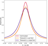 |
Fig. 1 Central peak of the etalon’s transmission profile for the three different configurations. The parameters of the etalon are R = 0.92, n = 2.29, d = 251 µm, ƒ# = 60, θ = 0° (collimated and perfect telecentric), and Θ = 0.3º (imperfect telecentric). |
3 Simulated observations
All the instruments built around the use of an etalon as a wavelength filtering element operate in a very similar way. They scan a spectral line by tuning the etalon (by changing the distance between mirrors and/or modifying the refractive index) to a desired number of wavelengths along the spectral line. At each spectral position, the solar scene is recorded. The measured intensity is approximately given by Eq. (4), with the etalon’s transmission profile centered at the desired wavelength.
We carried out a series of simulations of a spectral line observation in different conditions. We used the Kitt Peak FTS-Spectral-Atlas as the reference (Brault & Neckel 1987) and, specifically, the Fe I spectral line at 6173.3 Å. Each observation was composed of Nλ wavelengths, where the measured intensity was recorded. At every wavelength λs, the corresponding transmission profile of the etalon  was computed, and the “observed” intensity
  corresponding to a specific spatial location (ξ, η), represented hereinafter by the pixel i, was calculated using Eq. (4). Additionally, we took into account the presence of additive Gaussian noise. This noise does not necessarily respond to any parameter fluctuation within our analytical expressions or photon noise but comes from any unexpected variations that may not have been modeled in the theoretical scheme.
Additionally, we included the presence of defects arising from irregularities or inhomogeneities on either the cavity thickness d, the refractive index n, or from deviations of the angle of incidence θ. In order to simulate this, we introduced a relative perturbation ∆a into the etalon equation that accounts for any local deviation of the value of a with respect to its nominal value. This parameter changes from pixel to pixel differently for the collimated and telecentric configurations. In the former, the profile shifts across the FoV only because of the different incidence angles of the light beam on the etalon. In the latter, local variations of n and/or d are mapped directly onto the detector. We also note that variations in the incidence angle must be considered as well when the degree of telecentrism varies along the detector. Analytically, the parameter a at each i-th pixel is given by a′i = a∆ai, where a = (2π/λ)nd cos θ is constant along the FoV.
We let  be the noise contribution at the ith pixel and wavelength λs. Thus, the observed intensity at that pixel when the etalon is tuned at
  is given by
 (10)
(10)
with λc being the continuum wavelength. From a practical point of view, the integration limits are set in such a way that only a single resonance (or order) of the etalon is included with the limits, thus, acting akin to the sorting pre-filter commented on previously. We note that the denominator strictly corresponds to the intensity at the continuum of the line in the absence of the transmission profile or if the continuum wavelength is far enough from the spectral line. In any other case, the transmission should be taken into account as well to normalize the observations to the local continuum, which is necessary since we work with relative measurements. An example of a spectral line measurement is displayed in Fig. 2.
For both the collimated and telecentric configurations, we modeled etalon and gain imperfections over a 100 × 100 px2 image. Pixel-to-pixel variations in the sensor efficiency were modeled following a random spatial distribution, as shown in Fig. 3 (top panel). Additionally, we included a set of pixels with very low gain values, which represent a group of dead pixels or dust grains.
We modeled the etalon defects as changes in ∆a in such a way that the maximum displacement reaches 3 pm. The spatial distribution of the values of ∆a follows an increasing radial distribution, as shown in Fig. 3 (bottom panel). Such a spatial distribution coincides with the expected one in collimated etalons due to the change in the incidence angle across the FoV.
Telecentric mounts do not exhibit a spatial distribution of their defects such as this, but using the same spatial distribution in the two cases allowed us to compare the performance of the method for both setups in a systematic way. Since ∆a accounts for relative perturbations, it is by definition an adimensional parameter. However, to grant it a physical meaning, we express the values of ∆a in Å, representing the associated shift of the transmission profile with respect to the original position determined by a.
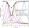 |
Fig. 2 Simulated observation of the Fe I spectral line (λ0 = 6173.3 Å) using a collimated mount and a total of Nλ = 6 wavelengths that have been equally distributed along the spectral line, with the exception of the continuum measurement (light blue), which is selected at 300 mÅ from the blue of the line core. The measured intensity is the result of computing the value given by Eq. (10) at each wavelength and with 𝑔=1. |
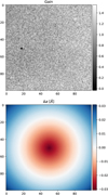 |
Fig. 3 Input maps introduced when simulating the observations. The top panel represents the gain generated as white Gaussian noise, with values ranging from 0.8 to 1.2. A dust speck was introduced by creating a group of four pixels with low values of 𝑔 = 0.2 for the gain. The bottom panel shows the spatial distribution of the defects in the etalon. The distribution follows a radial pattern starting from the center of the FoV. The defects vary from 0% deviation to up to 5 × 10⁻⁴%, which corresponds to a shift of 3 pm. Both possible directions for the deviations have been considered. The sign of the deviation is negative at the very center, which introduces a redshift, while it is positive at the corners, causing a shift of the profile into the blue. |
4 Fitting algorithm
We have developed an algorithm able to extract the distribution of the etalon defects and the gain map from data taken by etalon-based instruments, which enables the correction of the two contributions separately. The algorithm works by minimizing a given merit function that depends on the gain and the etalon defects.
In particular, we have defined an error metric, ελ, at each tuned wavelength, computed by comparing the measured intensity with the theoretical prediction. If we let  be the measured intensity at a given i pixel for an etalon tuned to the wavelength λs, the error metric at each wavelength is given by
 (11)
(11)
The merit function we employed is then the quadratic summation of the error metric over all tuned wavelengths:
 (12)
(12)
Both the camera gain and the defects of the etalon change from one pixel to another, which is why we address each pixel independently, but they remain constant at every wavelength. Hence, the transmission profile of the etalon varies at different points of the FoV; but at a given pixel, it is constant at all tuned wavelengths. Therefore, the algorithm is able to better obtain the etalon properties as we increase the number of wavelengths.
Figure 4 shows the derivatives of the error metric, Eq. (11), as a function of wavelength, that is, before computing the summation over s of the merit function, with respect to the gain, the reflectivity, and ∆a. The curve corresponding to the ∆a derivative is different from the others, whereas the derivatives of both the gain and the reflectivity exhibit similar shapes. Hence, variations in either the reflectivity or the gain introduce similar changes in the merit function, which can produce a trade-off between these two parameters, especially when the spectral line is sampled in only a few points. Given that discrepancies arising from errors in reflectivity are assimilated by gain maps, we did not take into account reflectivity errors when computing our simulations, as they have no impact on cavity map calculations.
A few key aspects arise when analyzing the merit function and its applicability on real data. The first point to bear in mind is that the shape of the object, O(λ), is not known a priory. Therefore, we needed to provide a guess for it. The method works by assuming that differences between the prediction and the observation are caused exclusively by the etalon defects or the gain. If the object used during the fitting process differs considerably from the real one, the prediction and observation will have differences that will erroneously be identified as etalon defects or gain variations. This is the main source of errors for the method when applied to real data. Two approaches can be followed in order to address this issue. The first one consists of assuming the solar atlas profile as the object. This is a good approximation, provided the data to which the algorithm is applied to lack information about solar structure, either because they are observations of long integration times of the quiet sun or produced by averaging several quiet sun observations (flat fields). If this condition cannot be met, this approach is not valid. The second approach involves deriving an approximated object from the data themselves by deconvolving the mean profile of the observation with the etalon’s transmission profile. This approach can account for any difference the real object may have with the solar atlas and thus has a greater resemblance to the real object. Nevertheless, the process of deconvolving is prone to errors when the sampling is insufficient and can introduce additional noise into the problem. We have tested both approaches to compare their performances on different scenarios in order to assess when to use one or the other.
We employed Newton’s method to minimize the merit function, Eq. (12), as it has been proven to quickly converge (in five iterations or fewer, usually). The method begins by assuming an initial guess for the gain 𝑔j and ∆aj parameters. Then, provided the initial guess is sufficiently close to the solution and that the merit function is continuous and differentiable, the gain 𝑔j and ∆aj encoded in the vector, xj, can be updated iteratively at each iteration, j, as
 (13)
(13)
where ℋ and 𝒿 are the Hessian and Jacobian matrices of the merit function ƒ, respectively, calculated for xj = [𝑔j, ∆aj]⊤ and⊤ stands for the transpose. Hence, the transmission profile of the etalon and its derivatives have to be computed for every wavelength and every pixel at each iteration. This can be computationally costly, especially when using imperfect telecentric configurations, where numerical integrals are involved.
All derivatives needed for the algorithm are calculated analytically, except when simulating imperfect telecentrism. A detailed formulation of these derivatives is provided in the appendix.
Regarding the object O(λ), if we assume it is given by the solar atlas, no additional computations are needed. However, when using the deconvolution approach, the object has to be calculated in each iteration. In this case, the algorithm works as follows: First, we compute the average profile across the whole FoV, and we force the continuum intensity to be the same on both sides of the spectral range to reduce the boundary effects of the deconvolution. This step is only necessary in case the spectral line is sampled in only a few positions, as is the case of the SO/PHI, IMaX, or TuMag instruments, where only a continuum point, either at the red or the blue side of the spectrum, is recorded. Both the object and transmission profile require a good spectral sampling to accurately compute the integrals of Eq. (11). Second, a cubic spline interpolation is applied to the generated average profile to artificially improve the spectral sampling, if necessary. Finally, the interpolated profile is then deconvolved by means of a Wiener filter with the etalon’s transmission profile. The result of this deconvolution is the object, O(λ), used in the minimization algorithm. The deconvolution of the object is done every time the etalon defects are updated in order to improve the resemblance of the deconvolved object to the real one. Figure 5 shows an example of this process in a simulated observation using nine scanned points and a collimated configuration. The deconvolution manages to reproduce the original signal, with only some minor differences in the line core and the beginning of the wings.
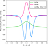 |
Fig. 4 Derivatives of the error metric as a function of wavelength. The derivative with respect to ∆a has been normalized in order to fit the three curves in the same plot. |
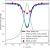 |
Fig. 5 Deconvolution of the object with a measurement of the Fe I spectral line using Nλ = 9. All points of the FoV have been used to compute the average profiles (red crosses). The deconvolution (blue) is the result of deconvolving the mean profile interpolation (dashed line) with the displayed etalon transmission profile (green). |
5 Test scenarios and results
The aim of the simulations carried out in this section was to characterize the role of the noise  , the spectral sampling, the selection of the object O(λ), and the accuracy of the method for both the collimated and telecentric configurations. All simulations were run for different choices of the number of scanned wavelengths, ranging from Nλ = 5 to Nλ = 21.
5.1 Impact of the noise level
We first assumed that the spectrum of the observed object is given by the solar atlas. This way, all errors in the derivation of the gain and etalon defects only come from the noise introduced into the measurement. We refer to this as the “ideal case.” Since we were combining different measurements taken at different wavelengths, we considered a worst-case scenario and simulated three different signal-to-noise ratios: 100, 150, and 200.
We restricted imperfections in the telecentrism to arise only for one scenario, S/N = 200, since simulating imperfections requires a high computational effort due to the lack of a theoretical expression for both the transmission profile and its derivatives. We also assumed that the degree of telecentrism (0.3°) is known in this case.
Figure 6 shows the average absolute error in 𝑔 (top panel) and in ∆a (bottom panel) over the whole FoV as a function of the wavelength sampling, Nλ. The error in 𝑔 is expressed as a percentage of its real value. Errors in ∆a are given in meters per second since they are mostly responsible for shifting the profile. Errors in ∆a can be translated into velocity errors with the center-of-gravity method (Uitenbroek 2003) through the expression
 (14)
(14)
where ∆λ is the spectral shift of the transmission peak produced by the error in ∆a.
All the scenarios exhibit a similar behavior as far as their dependence on the spectral sampling is concerned, namely, the absolute errors decrease monotonically when the wavelength sampling increases. The reason for this is simply that a larger number of wavelength samples increases the amount of available information that the algorithm can use, thus making the fitting for 𝑔 and ∆a more precise. These results highlight the importance of properly sampling the targeted spectral line. A modest sampling of only Nλ = 5 can produce errors as large as 120 m s−1 in the worst-case scenario (S/N = 100).
The noise level also plays an important role in the accuracy of the results. Scenarios with a lower S/N always have larger errors, for a given Nλ, in both the gain and ∆a computations. The difference in the performance of the algorithm due to the noise also changes with the spectral sampling; scenarios with a poor spectral sampling suffer from larger differences in the accuracy between the different S/N (50 m s−1 for Nλ = 5 between S/N = 200 and S/N = 100) than those with higher samplings (35 m s−1 for Nλ = 21).
The optical configuration of the etalon has a very small impact on the accuracy of the algorithm. Results for the three setups are very similar, particularly in the gain calculation, for which the results are almost identical for all configurations. Retrieval of ∆a is slightly better for the collimated mount, though.
Figure 7 shows the spatial distribution of the errors in the retrieval of ∆a for different choices of Nλ. There are no signs of a radial distribution in the maps shown in the figure, contrary to the actual distribution of the ∆a parameter, as shown in Fig. 3, bottom panel. This means that the precision of the method is similar no matter the amplitude of the defects, that is, we achieve the same accuracy in the retrieval of defects associated with shifts of 3 pm (~1450 m s−1, near the corners of our FoV), which correspond to cavity errors of around 1.5 nm or incidence angles of approximately 0.4 degrees, and in the retrieval of regions where no defect is present (radius of 20 pixels from the center of the FoV approximately). Instead of a radial distribution, the errors follow a Gaussian-like distribution (shown at the bottom panels in 7) similar to the one followed by the noise contribution.
The standard deviation of the errors for both the gain and ∆a computations are also reduced with an increase in spectral sampling. The last row of Fig. 7 displays the error distributions in the calculation of ∆a for the three optical configurations and different spectral samplings. These results illustrate how the three configurations yield practically identical results and how the distribution narrows as Nλ increases, thereby improving the results.
Specifically, the standard deviation decreases from 50 m s−1 for Nλ = 5 to 20 m s−1 for Nλ = 21. In the case of the gain determination, the standard deviation ranges between 0.2% and 0.1% for the scenarios with the poorest and highest spectral sampling, respectively.
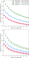 |
Fig. 6 Absolute errors of the gain (top) and etalon defect (bottom) derivations averaged over all the FoV. The number of wavelengths corresponds to the parameter Nλ of wavelengths used to scan the profile. |
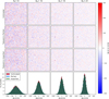 |
Fig. 7 Distribution of the errors in the ∆a computation for the three configurations (first three rows) and different spectral samplings (columns). In the bottom panels of each column, the error distribution for the corresponding spectral sampling is shown for the three configurations. |
5.2 Impact of the object approximation
To infer the error of the algorithm when the object is unknown, we compared the performance of the ideal case, that is, when the object used to generate the observations is known, with the one achieved when deconvolving the object from the data. Only the collimated setup was simulated in order to focus exclusively on the errors introduced by the deconvolution. The data has been degraded by Gaussian noise with an S/N = 200 in both scenarios.
Figure 8 shows the results for the two approaches. Interestingly, the error in the gain for the deconvolution approach does not decrease with a larger number of wavelengths, unlike the ideal case. Nevertheless, the average error of the calculation is below 0.4%, with a dispersion (1 σ) of ±0.3%. The decon-volution approach is prone to higher errors when deriving the gain due to the normalization of the profiles. The reason for this is two-fold. first, if the continuum is far enough from the spectral line, the normalization is strictly the integral over the transmission profile because the object is flat along the integration interval. However, this is not strictly true since the wings of the transmission profile can reach the spectral line (see Fig. 2), hence modifying the normalization of the profile when the object changes at each iteration. Second, should the continuum intensity of the derived object vary with respect to its real value due to the deconvolution process (e.g., due to boundary effects), there will be a shift in the intensity of the whole profile induced by the normalization process. These two effects seem to dominate the accuracy on the gain determination, regardless of the chosen sampling.
For ∆a, the performance of the method is slightly worse than for the ideal case when using the deconvolution approach. Unlike the gain determination, errors in the ∆a derivation show a strong dependence on the spectral sampling. Differences between both approaches range from 10 m s−1 to 40 m s−1 and increase with decreasing Nλ. The sensitivity with Nλ is especially high up to Nλ = 8. A modest increase of Nλ from five to six improves the determination of ∆a ~ 20 m s−1, whereas at better spectral samplings, the difference between each simulation decreases more slowly, without any relevant improvement as the sampling increases. In any case, differences are all well within ±1σ.
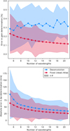 |
Fig. 8 Errors in gain determination and etalon properties averaged over all the FoV with a signal-to-noise ratio of 200 and a collimated configuration. |
5.3 The crossover case
The fact that the sensitivity of the model to the gain and to the ∆a parameters are different guarantees (to some extent) that the parameters can be separated from each other. The treatment of the problem is very different between etalon configurations, and therefore full knowledge of the setup is critical. However, this is not always feasible due to the unavoidable presence of errors, misalignment, and imperfections on the instrument. Approximations to describe the optical setup are also common in the pipeline of an FPI instrument because they reduce computational efforts. For instance, telecentric mounts are usually simplified as collimated setups, as the f-numbers employed in solar instruments are usually very large. Imperfections of telecentrism are commonly neglected, too. In this section, we analyze the impact of assuming an incorrect etalon mounting. To do so, we repeated the previous exercise, starting from a perfect and imperfect telecentric configuration but assuming that the transmission profile shape corresponds to a collimated one.
In this exercise, we assumed that we have an instrument with an FPI in a telecentric mount, as in the previous sections, in both perfect and imperfect configurations and an S/N = 200. We also considered that the object is given by the spectral solar atlas. The shift of the perfect telecentric transmission profile with respect to the collimated one was corrected using Eq. (52) from Bailén et al. (2019) to avoid the emergence of spurious velocity signals. Imperfections in the telecentrism shift the profile more. This additional displacement was left uncorrected intentionally so we could study its effects.
Figure 9 shows the error distributions for ∆a when the model assumes a collimated configuration for Nλ = 5 and Nλ = 21 and for both perfect and imperfect configurations. The amplitude and dispersion of the error distributions are very similar for the two mounts and are comparable to the results obtained in the ideal case (Fig. 7, bottom panel). The main difference between the perfect and imperfect scenarios is a shift of 130 m s−1 for the reason mentioned above. We note that this shift can easily be accounted for since it is a known and measurable effect.
The similarity in the error distributions for the calculation of ∆a in the two scenarios demonstrates that the error incurred when assuming a collimated etalon does not significantly impact the determination of the cavity maps of the etalon. This is because changes in ∆a mostly induce a shift of the transmission peak by an equal amount in both cases.
We note, however, that the amplitude, width, and shape of the transmission profile differ significantly between the telecentric and collimated configurations, leading to an expected higher error in gain calculation. Figure 10 shows the absolute errors in gain and ∆a calculations for both crossover scenarios and the ideal case after correcting the wavelength shift between the different mounts. For ∆a, the performance of the method is very similar in the three setups, as also observed earlier. This behavior is nevertheless anticipated since the properties selected for simulating the imperfect etalon were chosen to mirror those of the SO-PHI etalon, which were adjusted to closely resemble the behavior of a collimated etalon to the greatest extent possible.
The differences are larger for the gain determination. Not only are the errors higher in the crossover cases, but the trend is entirely different. Instead of decreasing when increasing the number of wavelengths, gain errors remain the same for the perfect case and increase with the number of samples for the imperfect case. Similar to the deconvolution case (Fig. 8), the difference between transmission profiles introduces an error in the normalization process that systematically affects the rest of the measurements. This effect becomes more pronounced as the number of wavelengths increases, given that this error is introduced more frequently, and it is even more prominent in the imperfect case, as not only are the profiles different in this scenario, but they are also asymmetric. This asymmetry results in an imbalance in the measurement of the profile, as one wing of the spectral line has a higher transmissivity and is observed with greater intensity than the other.
Our results suggest that assuming an etalon in a collimated configuration for instruments with telecentric mounts can be a good first-order approximation for cavity map calculations, provided that the level of asymmetry of the transmission profile is known. However, achieving an accurate knowledge of the degree of telecentrism is often challenging in real instruments, as it usually varies across the FoV. Meanwhile, the results highlight that this approximation leads to a considerable increase in the error in the gain determination, which increases when increasing the spectral sampling. This contrasts with the standard philosophy of solar instrumentation, which requires a high number of points to better scan the spectral line.
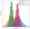 |
Fig. 9 Distribution of the errors in the determination of ∆a for the crossover scenarios (different configuration in the observation generation and minimization algorithm) for both perfect and imperfect configurations. Only results for the two extreme spectral samplings (Nλ = 5 and Nλ = 21) are shown. |
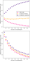 |
Fig. 10 Average errors of the gain (top panel) and etalon defect (bottom panel) calculations over all the FoV for the two crossover cases and the standard case (also shown in Fig. 6 as the collimated case with S/N = 200) for reference. All ∆a errors have been computed by correcting differential offsets of the transmission profile between the different mounts. |
5.4 Real data
While simulated tests are crucial for understanding the algorithm’s behavior as a function of the different parameters of the problem, tests with real data are required to validate the effectiveness of the method. In this section, we evaluate the results obtained by the algorithm when implemented on observations acquired using the High-Resolution Telescope (HRT) of the SO/PHI instrument.
The observation we used corresponds to a flat-field observation employing six points to scan the 6173 Å line (five along the spectral line and an additional continuum measurement) conducted on March 9, 2022. The FPI aboard SO/PHI is illuminated in a telecentric mount, with an expected degree of telecentrism of about 0.3°. The tests conducted with this dataset have the same procedure as the ones employed for simulated data, that is, we only fit the gain and ∆a parameters, and we employed the deconvolution approach (Sect. 5.2).
Figure 11 shows the results obtained when applying the algorithm to HRT-SO/PHI data. The top row shows, from left to right, the observed flat at the continuum, the cavity map measured under laboratory conditions (on ground), and a selected region of the cavity map. In the bottom row, the same cases are shown but for the results inferred by the algorithm. That is, the flat-field (i.e., the gain) and the cavity map (i.e., ∆a).
The results obtained for the cavity map closely resemble the laboratory measurements. The overall structure is preserved, maintaining the gradient from the upper left to the lower right. Similar structures are also discernible, such as the vertical line in the lower-right corner and the ring-like patterns evident in the lower section of the image. However, closer scrutiny of the observed structures revealed some differences. This deviation between results and measurements is expected, considering that the experiment conducted here represents a first-order approximation to assess the algorithm’s capability to generate coherent results. Several factors contribute to these differences. Firstly, the spatial resolution of the cavity measured on ground is lower. Secondly, the degree of telecentrism has a predicted variation of 0.23° across the FoV. Thirdly, we expected an error for the six-point scan, employing the deconvolution strategy, as large as a hundred meters per second.
Concerning the results for the gain determination, the comparison depicted in Fig. 11 suggests that pixel-to-pixel gain variations can also be determined accurately with our method, as both small-scale and large-scale variations are reproduced with detail.
A more quantitative analysis of the results is depicted in Fig. 12. The upper panel shows a comparison between the fitted and observed profiles for three distinct cases with varying degrees of precision, while the bottom panel shows the distribution of χ2 for all pixels. In the worst-case scenario, small differences between the real profile and the fit can be seen in both the line wing and the line core. In any other case, the fittings are rather satisfactory.
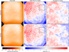 |
Fig. 11 Comparison between the observed flat-field and cavity map (top row, left and center columns, respectively) and the derived flat-field (gain) and cavity map (∆a; bottom row, left and center columns, respectively). The right column in both rows showcases a zoomed-in region of each cavity map. The area corresponding to the zoomed-in region is indicated with a black square in the full cavity map to its left. The properties used to simulate SO/PHI’s etalon are R = 0.925, n = 2.29, d = 251.63 µm, f# = 60, Θ = 0.23°. |
6 Conclusions
We have developed an algorithm that infers the gain and the etalon cavity map from flat-field observations along a spectral line. A series of simulated observations have been used to test the performance of the method. Real observations of HRT-SO/PHI were employed to validate our algorithm. Three different noise levels were considered in the simulations as well as different spectral samplings for the scanning of the spectral line. We applied the algorithm to three different optical configurations of the FPI: collimated, ideal (perfect) telecentrism telecentric, and imperfect telecentrism. The performance of the algorithm for the majority of scenarios seems robust enough for its applicability to real data, as verified by the results obtained with HRT-SO/PHI measurements.
The simulations that we carried out were aimed at testing different key aspects when assessing their applicability to real data. In the first place, the performance of the algorithm was tested as a function of the S/N of the observations, the spectral sampling, and the configuration of the etalon, assuming the spectrum of the object is known. We also studied the possibility of deriving the observed object from the data through a deconvolution process. We tested the performance of this approach as a function of the spectral sampling. Finally, we simulated a scenario in which the etalon configuration was different from the real one. The aim of these tests was to assess the impact of neglecting some properties of the etalon, such as the asymmetries in telecentric imperfect scenarios.
The algorithm has shown a high sensitivity to the noise level of the data. Nonetheless, the worst-case scenario considered in this work corresponds to much worse performances than current instruments can achieve in terms of S/N, and the errors are still within the necessary limits. In addition, the performance of the algorithm is the same for regions of the FoV where the etalon properties are far from their nominal values and regions where there is no deviation of the etalon properties.
Results for the three different optical configurations of the etalon are very similar. The telecentric configuration showed a worse performance than the collimated one in terms of cavity map retrieval. The loss of precision is nonetheless very small, below ~5 m s−1 in most cases.
The deconvolution of the object during the calculations was shown to yield a performance close to the ideal case in terms of cavity map determination. The performance when computing the gain showed a different behavior, although the average error never exceeds 0.4%. Concerning the dependence on the spectral sampling, the results show that with a scanning of at least six points, the additional error of deconvolving the object will not be larger than 25 m s−1. Overall, we estimated a total error smaller than 100 m s−1 for the worst-case scenario, where only five wavelengths are used to scan the line using the deconvolution approach for an S/N of 200.
In real instruments, light travels through different optical elements before reaching the etalon. Along this light path, the observed object might be modified in such a way that it no longer resembles a fixed reference. It is in fact very difficult to assess the error associated with this assumption (i.e., assuming that the object reaching the etalon is that of the FTS atlas profile) since these deviations cannot be measured. By deriving the object from the data, we expect additional errors due to the deconvolution process of around 10 m s−1, which we expect to be smaller than the ones produced by selecting a fixed object that differs considerably from the real one. Additionally, the deconvolution of the object allowed us to apply the algorithm to data where a solar structure is partly present.
Knowledge of the exact shape of the transmission profile has proven to be relevant to ensuring the accuracy of the algorithm. The results obtained for the crossover scenario have demonstrated that approximating the FPI’s transmission profile by another can serve as a first-order approximation. However, the determination of the gain has proven to be much more sensitive to changes in the transmission profile. The errors observed in the crossover scenario are higher overall than those of the ideal case. In addition, the unaccounted asymmetries of the imperfect configuration paradoxically increase the error when improving the spectral sampling.
The results obtained when applying the algorithm to real observations taken with SO/PHI reinforce the validity of the algorithm. Indeed, we have been able to extract the contribution of the cavity map from the flat-field observations. Comparison of the derived cavity map with lab measurements suggests that the algorithm can successfully extract the cavity map from the flat-field observations. In future works, we aim to allow the algorithm to modify the angle of incidence across the FoV and validate the results by implementing them in the SO/PHI pipeline.
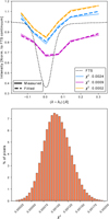 |
Fig. 12 Comparison between the measured (solid lines) and fitted profiles (dashed lines) for three pixels, each representing varying degrees of accuracy (top panel). The FTS is shown as a reference. The bottom panel displays the distribution of χ2 values for all pixels. Among the three selected cases, one demonstrates an average fit (depicted in pink, with χ2 close to the mean value), while the other two correspond with extreme cases—one with a notably good fit and the other with a poor fit (depicted in yellow and blue, respectively). The value for χ2 has been computed employing Eq. (12). |
Acknowledgements
This work is funded by AEI/MCIN/10.13039/501100011033/ (RTI2018-096886-C5, PID2021-125325OB-C51) and ERDF “A way of making Europe”; “Center of Excellence Severo Ochoa” awards to IAA-CSIC (SEV-2017-0709, CEX2021-001131-S).
Appendix Merit function derivatives
In this appendix, we present the derivatives of the merit function (12), which are required for calculating the Hessian and Jacobian matrices. Additionally, we provide the derivatives of the transmission profile for both the collimated and perfect telecentric configurations.
We show the derivatives of the merit function with respect to ∆a and g, since these are the parameters we have employed in all tests of this manuscript. These derivatives are the following:
![Mathematical equation: ${{\partial f(\Delta a,g)} \over {\partial \Delta a}} = \sum\limits_{s = 0}^{{N_\lambda }} {\left\{ { - g\left[ {{{\int {{\partial _{\Delta a}}} {\Psi ^{{\lambda _s}}}(\lambda ,\Delta a)O(\lambda ){\rm{d}}\lambda \int {{\Psi ^{{\lambda _c}}}} (\lambda ,\Delta a)O(\lambda ){\rm{d}}\lambda } \over {{{\left( {\int {{\Psi ^{{\lambda _c}}}} (\lambda ,\Delta a)O(\lambda ){\rm{d}}\lambda } \right)}^2}}} - {{\int {{\Psi ^{{\lambda _s}}}} (\lambda ,\Delta a)O(\lambda ){\rm{d}}\lambda \int {{\partial _{\Delta a}}} {\Psi ^{{\lambda _c}}}(\lambda ,\Delta a)O(\lambda ){\rm{d}}\lambda } \over {{{\left( {\int {{\Psi ^{{\lambda _c}}}} (\lambda ,\Delta a)O(\lambda ){\rm{d}}\lambda } \right)}^2}}}} \right]} \right\}} ,$](/articles/aa/full_html/2024/08/aa49825-24/aa49825-24-eq21.png) (15)
(15)
and,
 (16)
(16)
where we have used the notation ∂∆a := ∂/∂∆a for simplicity.
The derivatives for the transmission profiles with respect to ∆a are
 (17)
(17)
for the collimated case, and,
![Mathematical equation: ${{\partial {\Psi ^{{\lambda _s}}}(a(\Delta a))} \over {\partial \Delta a}} = {{{\Psi ^{{\lambda _s}}}(a(\Delta a))} \over {\partial a}}{{\partial a} \over {\partial \Delta a}} = 2\left( {\Re [E(a(\Delta a))]{{\partial \Re [E(a(\Delta a))]} \over {\partial a}} + \Im [E(a(\Delta a))] + {{\partial \Im [E(a(\Delta a))]} \over {\partial a}}} \right){{\partial a} \over {\partial \Delta a}},$](/articles/aa/full_html/2024/08/aa49825-24/aa49825-24-eq24.png) (18)
(18)
for the perfect telecentric configuration. The derivatives for the real and imaginary parts of E(a(∆a)) are
![Mathematical equation: ${{\partial \Re {\rm{e}}[E(a(\Delta a))]} \over {\partial a}} = {{2\sqrt \tau } \over {{\alpha _1}}}\left[ {{{\alpha _1^\prime } \over {{\alpha _1}}}\left( {\arctan {\gamma _2} - \arctan {\gamma _1}} \right) + {{\gamma _1^\prime } \over {1 + \gamma _1^2}} - {{\gamma _2^\prime } \over {1 + \gamma _2^2}}} \right]{\rm{, }}$](/articles/aa/full_html/2024/08/aa49825-24/aa49825-24-eq25.png) (19)
(19)
and,
![Mathematical equation: $\eqalign{ & {{\partial [E(a(\Delta a))]} \over {\partial a}} = {{2\sqrt \tau } \over {{\alpha _2}}}{{1 + R} \over {1 - R}}\left[ {{{\alpha _2^\prime } \over {{\alpha _2}}}\left\{ {\ln \left( {{{{{\left( {1 + {\gamma _3}} \right)}^2} + \gamma _5^2} \over {{{\left( {1 - {\gamma _3}} \right)}^2} + \gamma _5^2}}} \right) - \ln \left( {{{{{\left( {1 + {\gamma _3}} \right)}^2} + \gamma _4^2} \over {{{\left( {1 - {\gamma _3}} \right)}^2} + \gamma _4^2}}} \right)} \right\} + {{8{\gamma _3}{\gamma _5}\gamma _5^\prime } \over {\left[ {{{\left( {1 + {\gamma _3}} \right)}^2} + \gamma _5^2} \right]\left[ {{{\left( {1 - {\gamma _3}} \right)}^2} + \gamma _5^2} \right]}} - } \right. \cr & \,\,\,\,\,\,\,\,\,\,\,\,\,\,\,\,\,\,\,\,\,\,\,\,\,\,\,\,\,\,\,\,\,\,\,\,\,\,\,\,\,\,\,\,\,\,\,\,\,\,\,\,\,\,\,\,\,\,\,\,\,\,\,\,\,\,\,\,\,\,\,\,\,\,\,\,\,\,\,\,\,\,\,\,\,\,\,\,\,\,\,\,\,\,\,\,\,\,\,\,\,\,\,\,\,\,\,\,\,\,\,\,\,\,\,\,\,\,\,\,\,\,\,\,\,\,\,\,\,\,\,\,\,\,\,\,\,\,\,\,\,\,\,\,\,\,\,\,\,\,\,\,\,\,\,\,\,\,\,\,\,\,\,\,\,\,\,\,\,\,\,\,\,\,\,\,\,\,\,\,\left. {{{8{\gamma _3}{\gamma _4}\gamma _4^\prime } \over {\left[ {{{\left( {1 + {\gamma _3}} \right)}^2} + \gamma _4^2} \right]\left[ {{{\left( {1 - {\gamma _3}} \right)}^2} + \gamma _4^2} \right]}}} \right]{\rm{, }} \cr} $](/articles/aa/full_html/2024/08/aa49825-24/aa49825-24-eq26.png) (20)
(20)
with the derivatives of the αn and γn parameters being
![Mathematical equation: $\eqalign{ & \matrix{ {\alpha _1^\prime = 2b\sqrt F ,} \hfill \cr {\alpha _2^\prime = 4b\sqrt {F(F + 1)} ,} \hfill \cr {\gamma _1^\prime = \sqrt F \cos \left( {{a_{\rm{s}}}({\rm{\Delta }}a),} \right.} \hfill \cr } \cr & \matrix{ {\gamma _2^\prime = \sqrt F (1 - b)\cos \left( {{a_{\rm{s}}}({\rm{\Delta }}a)[1 - b]} \right),} \hfill \cr {\gamma _4^\prime = {{1 - b} \over {2\sqrt {F + 1} }}{{\sec }^2}\left( {{{{a_{\rm{s}}}({\rm{\Delta }}a)} \over 2}[1 - b]} \right),} \hfill \cr {\gamma _5^\prime = {1 \over {2\sqrt {F + 1} }}{{\sec }^2}\left( {{{{a_{\rm{s}}}({\rm{\Delta }}a)} \over 2}} \right).} \hfill \cr } \cr} $](/articles/aa/full_html/2024/08/aa49825-24/aa49825-24-eq27.png) (21)
(21)
References
- Bailén, F. J., Suárez, D. O., & del Toro Iniesta, J. 2019, ApJS, 241, 9 [CrossRef] [Google Scholar]
- Bailén, F. J., Suárez, D. O., & del Toro Iniesta, J. 2021, ApJS, 254, 18 [CrossRef] [Google Scholar]
- Barthol, P., Gandorfer, A., Solanki, S. K., et al. 2011, Solar Phys., 268, 1 [NASA ADS] [CrossRef] [Google Scholar]
- Beckers, J. 1998, A&ASS, 129, 191 [NASA ADS] [CrossRef] [EDP Sciences] [Google Scholar]
- Brault, J., & Neckel, H. 1987, Spectral Atlas of Solar Absolute Disk-Averaged and Disk-Center Intensity from 3290 to 12510 Å. (tape-copy from KIS IDL library) [Google Scholar]
- Gonsalves, R. A. 1982, Opt. Eng., 21, 829 [NASA ADS] [CrossRef] [Google Scholar]
- Martínez Pillet, V., Del Toro Iniesta, J., Álvarez-Herrero, A., et al. 2011, Solar Phys., 268, 57 [CrossRef] [Google Scholar]
- Müller, D., Cyr, O. S., Zouganelis, I., et al. 2020, A&A, 642, A1 [NASA ADS] [CrossRef] [EDP Sciences] [Google Scholar]
- Noda, C. Q., Ramos, A. A., Suárez, D. O., & Cobo, B. R. 2015, A&A, 579, A3 [NASA ADS] [CrossRef] [EDP Sciences] [Google Scholar]
- Noda, C. Q., Schlichenmaier, R., Rubio, L. B., et al. 2022, A&A, 666, A21 [NASA ADS] [CrossRef] [EDP Sciences] [Google Scholar]
- Puschmann, K. G., Denker, C. J., Balthasar, H., et al. 2013, Opt. Eng., 52, 081606 [CrossRef] [Google Scholar]
- Rimmele, T. R., Warner, M., Keil, S. L., et al. 2020, Solar Phys., 295, 1 [NASA ADS] [CrossRef] [Google Scholar]
- Scharmer, G. 2006, A&A, 447, 1111 [NASA ADS] [CrossRef] [EDP Sciences] [Google Scholar]
- Scharmer, G. B., Narayan, G., Hillberg, T., et al. 2008, ApJ, 689, L69 [Google Scholar]
- Scharmer, G. B., de la Cruz Rodriguez, J., Sütterlin, P., & Henriques, V. M. 2013, A&A, 553, A63 [NASA ADS] [CrossRef] [EDP Sciences] [Google Scholar]
- Schmidt, W., Von der Lühe, O., Volkmer, R., et al. 2012, The 1.5 meter Solar Telescope GREGOR [Google Scholar]
- Schmidt, W., Schubert, M., Ellwarth, M., et al. 2016, in Ground-based and Airborne Instrumentation for Astronomy VI, 9908, SPIE, 1473 [Google Scholar]
- Schnerr, R., de la Cruz Rodriguez, J., & van Noort, M. 2011, A&A, 534, A45 [NASA ADS] [CrossRef] [EDP Sciences] [Google Scholar]
- Solanki, S. K., del Toro Iniesta, J., Woch, J., et al. 2020, A&A, 642, A11 [NASA ADS] [CrossRef] [EDP Sciences] [Google Scholar]
- Uitenbroek, H. 2003, ApJ, 592, 1225 [Google Scholar]
- van Noort, M. 2017, A&A, 608, A76 [NASA ADS] [CrossRef] [EDP Sciences] [Google Scholar]
- Van Noort, M., Der Voort, L. R. V., & Löfdahl, M. G. 2005, Solar Phys., 228, 191 [NASA ADS] [CrossRef] [Google Scholar]
All Figures
|
Fig. 1 Central peak of the etalon’s transmission profile for the three different configurations. The parameters of the etalon are R = 0.92, n = 2.29, d = 251 µm, ƒ# = 60, θ = 0° (collimated and perfect telecentric), and Θ = 0.3º (imperfect telecentric). |
| In the text | |
|
Fig. 2 Simulated observation of the Fe I spectral line (λ0 = 6173.3 Å) using a collimated mount and a total of Nλ = 6 wavelengths that have been equally distributed along the spectral line, with the exception of the continuum measurement (light blue), which is selected at 300 mÅ from the blue of the line core. The measured intensity is the result of computing the value given by Eq. (10) at each wavelength and with 𝑔=1. |
| In the text | |
|
Fig. 3 Input maps introduced when simulating the observations. The top panel represents the gain generated as white Gaussian noise, with values ranging from 0.8 to 1.2. A dust speck was introduced by creating a group of four pixels with low values of 𝑔 = 0.2 for the gain. The bottom panel shows the spatial distribution of the defects in the etalon. The distribution follows a radial pattern starting from the center of the FoV. The defects vary from 0% deviation to up to 5 × 10⁻⁴%, which corresponds to a shift of 3 pm. Both possible directions for the deviations have been considered. The sign of the deviation is negative at the very center, which introduces a redshift, while it is positive at the corners, causing a shift of the profile into the blue. |
| In the text | |
|
Fig. 4 Derivatives of the error metric as a function of wavelength. The derivative with respect to ∆a has been normalized in order to fit the three curves in the same plot. |
| In the text | |
|
Fig. 5 Deconvolution of the object with a measurement of the Fe I spectral line using Nλ = 9. All points of the FoV have been used to compute the average profiles (red crosses). The deconvolution (blue) is the result of deconvolving the mean profile interpolation (dashed line) with the displayed etalon transmission profile (green). |
| In the text | |
|
Fig. 6 Absolute errors of the gain (top) and etalon defect (bottom) derivations averaged over all the FoV. The number of wavelengths corresponds to the parameter Nλ of wavelengths used to scan the profile. |
| In the text | |
|
Fig. 7 Distribution of the errors in the ∆a computation for the three configurations (first three rows) and different spectral samplings (columns). In the bottom panels of each column, the error distribution for the corresponding spectral sampling is shown for the three configurations. |
| In the text | |
|
Fig. 8 Errors in gain determination and etalon properties averaged over all the FoV with a signal-to-noise ratio of 200 and a collimated configuration. |
| In the text | |
|
Fig. 9 Distribution of the errors in the determination of ∆a for the crossover scenarios (different configuration in the observation generation and minimization algorithm) for both perfect and imperfect configurations. Only results for the two extreme spectral samplings (Nλ = 5 and Nλ = 21) are shown. |
| In the text | |
|
Fig. 10 Average errors of the gain (top panel) and etalon defect (bottom panel) calculations over all the FoV for the two crossover cases and the standard case (also shown in Fig. 6 as the collimated case with S/N = 200) for reference. All ∆a errors have been computed by correcting differential offsets of the transmission profile between the different mounts. |
| In the text | |
|
Fig. 11 Comparison between the observed flat-field and cavity map (top row, left and center columns, respectively) and the derived flat-field (gain) and cavity map (∆a; bottom row, left and center columns, respectively). The right column in both rows showcases a zoomed-in region of each cavity map. The area corresponding to the zoomed-in region is indicated with a black square in the full cavity map to its left. The properties used to simulate SO/PHI’s etalon are R = 0.925, n = 2.29, d = 251.63 µm, f# = 60, Θ = 0.23°. |
| In the text | |
|
Fig. 12 Comparison between the measured (solid lines) and fitted profiles (dashed lines) for three pixels, each representing varying degrees of accuracy (top panel). The FTS is shown as a reference. The bottom panel displays the distribution of χ2 values for all pixels. Among the three selected cases, one demonstrates an average fit (depicted in pink, with χ2 close to the mean value), while the other two correspond with extreme cases—one with a notably good fit and the other with a poor fit (depicted in yellow and blue, respectively). The value for χ2 has been computed employing Eq. (12). |
| In the text | |
Current usage metrics show cumulative count of Article Views (full-text article views including HTML views, PDF and ePub downloads, according to the available data) and Abstracts Views on Vision4Press platform.
Data correspond to usage on the plateform after 2015. The current usage metrics is available 48-96 hours after online publication and is updated daily on week days.
Initial download of the metrics may take a while.