| Issue |
A&A
Volume 688, August 2024
|
|
|---|---|---|
| Article Number | A62 | |
| Number of page(s) | 13 | |
| Section | Stellar structure and evolution | |
| DOI | https://doi.org/10.1051/0004-6361/202346942 | |
| Published online | 02 August 2024 | |
A benchmark rapidly oscillating chemically peculiar (roAp) star: α Cir
1
Department of Astrophysics, University of Vienna, Türkenschanzstrasse 17, 1180 Vienna, Austria
e-mail: This email address is being protected from spambots. You need JavaScript enabled to view it.
2
Institute of Physics, University of Graz, 8020 Graz, Austria
3
Department of Physics and Astronomy, Vanderbilt University, Nashville, TN 37235, USA
Received:
19
May 2023
Accepted:
12
April 2024
Abstract
Context. The brightest chemically peculiar magnetic (mCP) star, α Cir, is also pulsating. Precise photometric and spectroscopic data, preferably with a long time base, are needed to investigate its evolutionary aspects as well. The present investigation of α Cir offers a space-based high-precision photometry study with high time resolution, covering 20+ years and supplemented by high resolution spectroscopy from the ground.
Aims. We discuss the controversial rotation periods that have been recently reported and we consider new determinations of the actual values. We process the complex pulsation frequency spectrum, considering the implications in modelling the structure of α Cir.
Methods. We developed an automated Bayesian algorithm to consistently search for periodic signals in the WIRE, SMEI, TESS, and BRITE space photometric datasets, complemented by radial velocity data from HARPS.
Results. New observations in 2021 and 2023 from TESS and BRITE indicate a detection of α Cir as a triple system. The rotation period of α CirA has been determined as 4.4792890 ± 0.0000018 d. The TESS data show a rich frequency spectrum including three l = 0, six l = 1, two l = 2, and one l = 3 modes. Of these, five are shown to be rotationally split. The dipole modes show significant curvature in the echelle diagram, probably due to the strong magnetic field of α Cir.
Conclusions. Overall, α Cir continues to be a cornerstone of mCP stars. A confirmation of the triple system requires additional space photometry and/or high-resolution spectroscopy to increase the time base. These data are also needed to improve the quality of the pulsation frequency spectrum and to investigate the evolutionary effects at play. A detailed seismic modelling study that considers the effects of a magnetic field on pulsation is subsequently recommended.
Key words: stars: chemically peculiar / stars: fundamental parameters / stars: interiors / stars: late-type / stars: oscillations
© ESO 2024
 Open Access article, published by EDP Sciences, under the terms of the Creative Commons Attribution License (http://creativecommons.org/licenses/by/4.0), which permits unrestricted use, distribution, and reproduction in any medium, provided the original work is properly cited.
1. Introduction
As a prominent member of the rapidly oscillating chemically peculiar (roAp) stars, α Cir has a strong magnetic field (mCP). Even though mCP stars have stood as a research focus for decades (e.g. Weiss et al. 1976), as illustrated by numerous research papers and workshops, there are still unsolved and controversial issues concerning their structure and evolution (see, e.g. the review by Kurtz 2022).
Generally, roAp stars pulsate in acoustic modes with low spherical degrees and high radial overtones and periods from a few to several tens of minutes. A peculiarity of these stars is a misalignment of the pulsation axis to the rotation as well as the magnetic axis. This led to the development of the oblique pulsator model (e.g. Kurtz 1982; Shibahashi & Saio 1985), suggesting that a pulsation mode, viewed over the rotation cycle of the star, shows changing aspects and leads to an apparent modulation of the pulsation amplitude. This model has been used and improved during the course of the last four decades and it is now facing new challenges on the back of recent TESS observations (e.g. Kurtz & Holdsworth 2020; Holdsworth et al. 2021)
Since the discovery of α Cir as a pulsating chemical peculiar star (Kurtz & Cropper 1981), more than 40 papers have been published, offering insights into various aspects of photometry and/or spectroscopy of this star and consequences for its modelling. This discussion led to the qualification of α Cir as a benchmark roAp star, however a full consideration of this context is beyond the scope of the present paper. We briefly refer in the following to papers related to aspects that are relevant for the present analysis.
The first paper in this sequence is from Kurtz (1982), who reported on the discovery of pulsation of α Cir, based on Johnson B photometry in 1981, and initiated the more than 40 years of research devoted to this star. A follow-up paper by Kurtz & Balona (1984) presented the first investigation of pulsation frequencies. These results were basically confirmed by Weiss & Schneider (1984), who published the first multi-colour Walraven photometry, Next, Schneider & Weiss (1989) used Stromgren photometry to discuss pulsation amplitude and phase shifts as a function of wavelength. Kurtz et al. (1994) detected rotational sidelobes to the main pulsation frequency and initiated attempts to determine the rotational period of α Cir, which is also the subject of the present analysis.
With time-resolved high-resolution spectra presented by Schneider & Weiss (1989), another topic was addressed. First, clear evidence for spectroscopic variability due to pulsation were provided by Baldry et al. (1998), who pointed to complex amplitude and phase variations of the principal pulsation mode, depending on the analysed spectral line (see also Balona & Laney 2003). A detailed abundance and stratification analysis of the stellar atmosphere was carried out by e.g. Kochukhov et al. (2009). A breakthrough was achieved when the High Accuracy Radial velocity Planet Searcher (HARPS) was installed at ESO in 2003. Mkrtichian & Hatzes (2013) initiated a campaign on α Cir, with data becoming available via the HARPS RV database (Trifonov et al. 2020).
The launch of the Wide Field Infrared Explorer (WIRE; e.g. Buzasi 2002), Solar Mass Ejection Imager (SMEI; e.g. Tarrant et al. 2008), BRIght Target Explorer (BRITE; Weiss et al. 2014), and Transiting Exoplanet Survey Satellite (TESS; Ricker et al. 2015) missions have offered new access to top quality, highly time-resolved, and long time-base photometry from space. In addition, BRITE-Constellation allows for a two-colour option, which significantly supports asteroseismic investigations. Hence, α Cir is one of its prime targets (Weiss et al. 2016).
Another important feature is the magnetic field of α Cir of about 1–2 kG (e.g. Bruntt et al. 2008), which has been discussed in the context of dipole oscillations in roAp stars by Bigot & Kurtz (2011) and critically investigated by Cunha et al. (2013). The latter argue that the oscillations of α Cir are clearly above the critical acoustic cutoff frequency, which is sensitive to the dynamics of the atmospheric layers of the star and where the magnetic field plays an important role. This evidence challenges the excitation models proposed by Balmforth et al. (2001).
In this paper, we focus on one of the prominent peculiarities of α Cir, which is pulsation. We also find indications for a hitherto unknown close second companion using recent photometric and spectroscopic observations. The potential of non-radial and multi-mode pulsation for studying the structure and evolutionary status of stars all over the HRD has become evident in these days and asteroseismology was established as a very powerful research tool (e.g. Gough 1985). The limitations of ground based observations, however, are serious (e.g. day-night cycles, weather gaps, seasons) and soon the potential of space observations was recognised (Aerts 2021).
All these papers and references provide evidences for α Cir being a treasure trove for studying roAp stars, as is also illustrated by Deal et al. (2021) who investigated the role of the large frequency separation, Δν, for modelling stellar properties. Seismic information infers the constrains for the internal chemical composition and the transport of chemical elements in Ap stars. Another example would be the recent surface mapping of α Cir, which indicates at least three spots with probably different chemical composition on its surface (Weiss et al. 2020).
In the following we investigate photometric time series obtained from space missions and spectroscopy from ground. Small but statistically significant long-term changes of the main pulsation frequency indicate a close low-mass companion of α Cir, which makes it a rare discovery of a secondary star only from the pulsation signal of the primary. Furthermore, we present the so far richest frequency spectrum of any roAp star and find no evidence for evolutionary changes of the stellar rotation period over about 40 years on a sub-ppm level.
2. Fundamental parameters of α Cir
Bruntt et al. (2008) carried out a detailed literature analysis and used high-resolution spectroscopic and interferometric measurements to determine accurate physical parameters of α Cir. Now, some 15 years later, we take the next step and perform an analysis of the broadband spectral energy distribution (SED) of the star together with the Gaia DR3 parallax (with no systematic offset applied; see, e.g. Stassun & Torres 2021), in order to determine an empirical measurement of the stellar radius, following the procedures described in Stassun & Torres (2016) and Stassun et al. (2017, 2018). We extracted the UBV magnitudes from Mermilliod (2006), the Strömgren uvby magnitudes from Paunzen (2015), the JHKS magnitudes from 2MASS, the W1–W4 magnitudes from WISE, and the GBPGRP magnitudes from Gaia. We discarded measurements that were clearly discrepant, either because of saturation due to the brightness of the source or because of poor quality flags reported in the catalogs. Finally, we also included the Gaia spectrum, which provides additional strong constraints on the bolometric flux due to the absolute flux calibration from space. Together, the available photometry spans the full stellar SED over the wavelength range 0.35–22 μm (see Fig. 1).
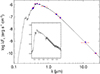 |
Fig. 1. Spectral energy distribution of α Cir. Red symbols represent the observed photometric measurements, where the horizontal bars represent the effective width of the passband. Blue symbols are the model fluxes from the best-fit PHOENIX atmosphere model (black). The Gaia spectrum is shown overlaid as a gray swathe (also shown in the inset plot). |
We performed a fit using PHOENIX stellar atmosphere models (Husser et al. 2013), with the free parameters being the effective temperature (Teff) and metallicity ([Fe/H]), and fixing the extinction to zero. The resulting fit (Fig. 1) has a best-fit Teff = 7450 ± 50 K, [Fe/H] = 0.3 ± 0.3, with a reduced χ2 of 0.6. Integrating the model SED gives the bolometric flux at Earth, Fbol = 1.289 ± 0.0.015 × 10−6 erg s−1 cm−2. Taking the Fbol together with the Gaia parallax directly gives the bolometric luminosity as Lbol = 10.80 ± 0.13 L⊙, from which the stellar radius follows via the Stefan-Boltzmann relation, R = 1.975 ± 0.030 R⊙. This value is in good agreement but about twice as accurate as the one determined by Bruntt et al. (2008) using α Cir’s angular diameter and Hipparcos parallax. In addition, we can estimate the stellar mass from the empirical eclipsing-binary based relations of Torres et al. (2010), resulting in M = 1.82 ± 0.11 M⊙. This is again consistent with the estimate from Bruntt et al. (2008) using an independent approach. Fundamental parameters are listed in Table 1.
Physical parameters of α Cir as determind in the present work.
3. Data
In the following we outline the time series observations from the various sources that are used in the present analysis. We apply a consistent data post-processing approach to minimise instrumental effects and to disentangle data used for the pulsation (Sect. 4) and rotation (Sect. 6) analysis for all time series, except for SMEI and HARPS. The method is described in detail in Sect. 3.1.
3.1. TESS
So far, α Cir has been observed with TESS Ricker et al. (2015) three times, between April and June 2019 as target in sector1 11 and 12, between April and June 2021 in sector 38 and 39, and between May and June 2023 in sector 65. For the present study, we use the 2-min cadence Pre-search Data Conditioning Simple Aperture Photometry (PDC_SAP) data provided by the TESS Science Processing Operations Center pipeline (Jenkins et al. 2016, SPOC) and accessible via the Mikulski Archive for Space Telescopes (MAST) at the Space Telescope Science Institute. Individual observations are only used if their quality flag is equal to zero and no further outliers are removed. The data are shown in Fig. 2.
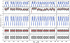 |
Fig. 2. TESS 2019 (left), 2021 (middle), and 2023 (right) light curves. Panels a: double harmonic fit (blue lines) to the original PDC_SAP data (grey dots). Panels b: original (grey dots) and heavily smoothed (red lines) residuals to the double harmonic fit of panels a. Panels c: original data corrected for the smoothed residuals from panels b (grey dots – these data are used for the rotation analysis) along with a double harmonic fit (blue lines). Panels d: original (grey dots) and heavily smoothed residuals (red lines) from panels c. Panels e: residuals from panels d. These data are used for the pulsation analysis. |
The average instrumental flux of the 2021 and 2023 data and their standard deviations σ differ significantly (by about 7 and 3%) from those of the 2019 data, which likely results from different apertures and/or background corrections used to extract the photometric time series. Ignoring such a difference could potentially affect the pulsation amplitudes in the subsequent analysis. We can however not simply correct for this effect as it is unknown to what extent it results from the aperture size (i.e. a multiplicative effect) or from the background correction (i.e. an additive effect). Luckily, the variations in both datasets are dominated by the rotational modulation, with an amplitude of proportional to the standard deviation (σ) of the time series. We therefore apply a correction factor of 0.973 to the 2021 data and of 0.968 to the 2023 data so that σ2023 ≃ σ2021 ≃ σ2019.
To minimise instrumental long-term trends in the time series, we fit amplitudes (an) and phases (ϕn) of a double harmonic function to the original time series according to:
![Mathematical equation: $$ \begin{aligned} f(t) = a_1 \cos \left( 2\pi \left[\frac{t}{P}+\phi _1 \right] \right) + a_2 \cos \left(2\pi \left[\frac{2t}{P} + \phi _2 \right] \right), \end{aligned} $$](/articles/aa/full_html/2024/08/aa46942-23/aa46942-23-eq1.gif) (1)
(1)
with a fixed period P = 4.47928 d. In a next step a second-order Savitzky-Golay filter, with a window length of about 2.8 d, is applied to the residual data. The resulting trend (see red lines in Fig. 2b) is then subtracted from the original data (Fig. 2c) giving the final time series used for the rotation analysis.
For the pulsation analysis we apply Eq. (1) again on the corrected data, but now use a shorter window length of about 6.7 h for smoothing. The final light curves are shown in Fig. 2e and have a point-to-point scatter2 of about 0.51, 0.50, and 0.49 ppt, respectively, which translates into a high-frequency Fourier noise of about 1.12, 1.07, and 1.30 ppm.
For the 2021 run also 20 s cadence data are available (Huber et al. 2022), which are supposed to be more precise than the 2–min cadence data for a star as bright as α Cir. However, we did not use them as the noise behaves quite differently for the sectors 38 and 39 and the final result from the frequency analysis is practically the same as for the 2–min cadence data.
3.2. WIRE
Soon after launch of WIRE in March 1999 the hydrogen cryogen boiled off due to a technical defect terminating the primary science mission. However, the onboard star tracker with 52 mm aperture remained functional and could be used for photometry till 2006 (e.g. Buzasi 2002), when communication with the satellite failed.
Altogether, α Cir was observed for a total of 84 days with the WIRE star-tracker in September 2000, February 2005, and February and July 2006. Bruntt et al. (2009) were the first to process the raw data and analyse the inherent pulsation signal, followed by Weiss et al. (2020) who used the same data primarily for spot modelling. The original data come at a very high cadence (below 1 s) but are binned to 15 s windows. In this work, we have re-assessed the Bruntt et al. (2009) data, but combining the February and July datasets of 2006 for an improved frequency resolution (see Table 2) and applying the same data post-processing as for the TESS data.
Photometry of α Cir from space and spectroscopy from ground.
3.3. SMEI
SMEI is an instrument on board the Coriolis satellite. The three CCD cameras of the instrument observe the whole sky in order to detect disturbances in the solar wind. Besides this primary science goal, the data were used to detect stellar pulsations in bright stars (e.g. Jackson et al. 2004). Altogether, α Cir was observed by SMEI for almost 2900 days between February 2003 and December 2010 (see Table 2). A single SMEI data point comes from a series of 4 s exposures, which are combined to windows of typically 1 min length. Raw SMEI data suffer from very strong instrumental effects so that data post-processing is a rather complicated procedure requiring multiple detrending and sigma clipping. The intrinsic low-amplitude pulsation signal remains inaccessible so that the final time series is binned to 100 min intervals. Weiss et al. (2020) provides more details on the procedure.
3.4. BRITE
Altogether, α Cir was observed in 2014 for a total of 145 d during the commissioning phase of BRITE-Constellation and the results were analysed by Weiss et al. (2016). Subsequent observations of the star were carried out in 2016 for 163 d by three of the five operational BRITE satellites, forming the basis for the investigations presented by Weiss et al. (2020). The photometric measurements and data reduction are described in the mentioned study.
In addition, α Cir was observed by BRITE-Toronto in the field 62-CruCar-III-2021, from late March to late August, 2021, for a total of 136 d. The satellite collected 10–30 measurements per ∼102 min satellite orbit, with a typical sampling rate of 20 s and an exposure time of 1 s. The raw images were processed using the pipeline described by Popowicz et al. (2017), which accounts for the technical issues that are typical for BRITE photometry, like hot pixels (Pablo et al. 2016). The extracted photometry3 still includes systematic instrumental effects due to CCD temperature drifts and the position of the star’s point spread function in the raster. These effects were minimised using the same approach as for TESS photometry, as described in Sect. 3.1. α Cir was also observed in 2018 with one of the BRITE satellites, but since the resulting time series is significantly shorter (∼65 d) and noisier than the other BRITE datasets, it does not contribute to the current analysis, which is why we decided to ignore it for the time being.
3.5. HARPS
Even though there are plenty of high-resolution spectroscopic observations available for α Cir, they are typically not suited for a detailed frequency analysis due to the usually short time base of hours up to a few days of the spectra. An exception are the more than 4800 echelle-spectra obtained during nine nights in February and April 2008 with the HARPS spectrograph of the European Southern Observatory’s 3.6-m telescope at La Silla. Exposure times were typically 20–30 s with a median sampling of 48 s. The campaign was presented by Mkrtichian & Hatzes (2013) stating that they detect 36 pulsation modes using an ’integral’ RV measurement based on individual spectral lines. Their results are in preparation now and the authors agreed (private communication) that we use the open-access radial velocity measurements from the HARPS database (Trifonov et al. 2020) for our purposes, which are automatically computed by cross-correlating with a numerical mask.
4. Pulsation
To extract the oscillation parameters from the light curves, we apply an updated version4 of the probabilistic approach presented by Kallinger & Weiss (2017). The automated Bayesian algorithm was originally developed to handle multiple close frequencies within the formal frequency resolution (Kallinger et al. 2017) but it works with a mono-periodic signal (within one formal frequency resolution bin) as well. The software uses the Python version (Buchner 2016, UltraNest) of the nested sampling algorithm MultiNest (Feroz et al. 2009) to search for periodic signals in time series data and tests their statistical significance by comparison with no signal (i.e. only noise). A solution is considered real5 (i.e. not due to noise) if its probability p = zsignal/(zsignal + znoise)≥0.91, where z is the global evidence6 delivered by UltraNest. The approach has been extensively tested with artificial data (Kallinger & Weiss 2017) and the subsequent results have been compared with those from Period04 (Lenz & Breger 2005). In all cases agreement was found within the uncertainties.
The dominant 6.8 min (≈2442 μHz) pulsation period is known for more than 40 years and has frequently been studied (e.g. Kurtz & Balona 1984; Schneider & Weiss 1983, 1989) after its discovery (Kurtz 1982). Rotational split components with δνrot = 2.593 ± 0.006 μHz next to the dominant frequency were first detected by Kurtz et al. (1994), based on the combination of multiple ground-based observing runs and later on confirmed by Bruntt et al. (2009) with WIRE data. However, the results of the two studies are inconsistent in a sense that frequencies found to be significant in one dataset do not show up in the other and vice versa. Meanwhile, this ambiguity is settled thanks to the high-precision time series of TESS.
4.1. TESS
Obviously, the most significant time series in the set of space photometry are those from the TESS satellite. Observations of α Cir were first reported by Holdsworth et al. (2021) as part of a systematic search for roAp stars in the southern hemisphere with TESS, but included no detailed analysis or interpretation of the data.
Using the above described Bayesian approach, we identified 17 significant (i.e. p ≥ 0.91) frequencies in the 2019 data (see Table 3), of which five modes (ν1, ν2, ν3, ν6, and ν7) show a clear triplet structure with an average split frequency of 2.586 ± 0.003 μHz. Five more frequencies ( ,
,  ,
,  ,
,  , and
, and  )7 are very close (∼0.2–0.6 μHz) to frequencies with a significantly larger amplitude indicating some long-period (∼20–50 d) amplitude and/or frequency modulation, which is not unusual for roAp stars (e.g. Holdsworth et al. 2021). For the sake of simplicity, we ignore them here, leaving a total of 12 independent pulsation frequencies. Figure 3 illustrates the original Fourier amplitude spectrum and the spectrum after prewhitening the first three frequencies. We note that all ten frequencies given by Holdsworth et al. (2021) are included in our list as well. In order to test if the data post-processing (Sect. 3) alters the result of the frequency analysis, we also analyse the raw PDC_SAP data but did not find any significant difference. Only the frequency and amplitude uncertainties are larger, especially for the low-amplitude signal.
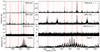 |
Fig. 3. Fourier amplitude spetra of the TESS 2019, WIRE 2006, combined BRITE 2014-16 light curves, and the HARPS radial velocities with the significant TESS frequencies overlaid as vertical red dotted lines. The original spectra are shown in the left panels, whereas right panels give the spectra after prewhitening the one to three most significant frequencies. |
Significant pulsation frequencies from TESS 2019 and 2021 observations.
Figure 4 presents the 2019 TESS frequencies in an echelle diagram. It shows that the five rotationally split modes (ν1, ν2, ν3, ν6, and ν7) are most likely of different spherical degree, l. They form (together with the non-split modes) at least two mode sequences of consecutive radial overtones of the same spherical degree. It is remarkable that the best populated sequence around ν1 is significantly curved even though high-radial order modes should rather follow a straight vertical line in the echelle diagram (Tassoul 1980).
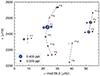 |
Fig. 4. Echelle diagram of the TESS 2019 frequencies with the (blue) symbol size indicating the mode amplitude and the annotation according to Table 3. Red and green symbols give the corresponding frequencies in the 2021 and 2023 dataset, respectively. Modes of presumably the same spherical degree are connected by dashed line segments. |
Analysing the 2021 data with the same significance criterion (i.e. p ≥ 0.91) reveals only part of the frequencies from 2019. In fact, six of the 27 previously significant frequencies remain undetected. However, lowering the probability threshold to p ≥ 0.72 gives three more frequencies that have already been detected in the 2019 data. Such a strategy might appear to increase the risk of collecting random noise peaks but is fully justified in a Bayesian sense as the sheer existence of a frequency in the 2019 data could serve as a prior in the 2021 analysis, which would increase the detection probability of this particular frequency. In total, only two of the low-amplitude frequencies ν9 and ν11 and the “modulation sidelobe”  remain undetected in the 2021 data. On the other hand, an additional significant frequency is consistent with the lower-frequency rotational sidelobe of ν12, which increases the number of rotationally split modes to six. We note that further lowering the probability threshold does not reveal the three missing frequencies. Obviously, at some point noise is taking over.
Since the 2023 dataset is only about half as long as the other two time series, we cannot expect the same level of detail as before. Using again a significance criterion of p ≥ 0.72, the Bayesian frequency analysis recovers, however, 18 of the 28 previously identified frequencies, including three triplets and two duplets. They are listed in Table 4 and illustrated in Fig. 4.
A closer look at the individual frequencies shows that nearly all have systematically decreased during the ∼2-year gap between the 2019 and 2021 observations. Even though there are some outliers, the change is generally highly significant and on average −21 ± 4 ppm (see Table 3, right-most column). Another interesting aspect is also that some of the amplitudes significantly decrease between 2019 and 2021 as well. While the change is quite moderate (−2 ± 0.5%) for the main frequency, the amplitudes of ν2 and ν3 decrease by more than 10%. The remaining frequencies are on the other hand generally stable within the uncertainties. Between 2023 and 2021, the frequencies and amplitudes seem to ‘recover’ again as they generally increase, even though not to the same level as in 2019 and with less significance (given the larger uncertainties of the individual measurements).
4.2. BRITE
As we have slightly modified the data processing of the BRITE photometry for the present analysis compared to Weiss et al. (2020), we re-analysed the pulsation signal. An additional dataset is now available, which makes a total of three (Table 2). Weiss et al. (2020) analysed the combined 2014 and 2016 BRITE data and found five significant frequencies. Here we are more interested in the temporal stability of the dominant frequency and, therefore, individually analyse the various datasets. In that sense, only ν1 and ν2 are statistically significant in the three BRITE datasets (Table 5).
Significant pulsation frequencies in the WIRE, BRITE, and HARPS observations derived in the present analysis and completed by literature values.
4.3. WIRE
In their pulsation analysis, Weiss et al. (2020) focused on the 2006 data of WIRE. Here, we re-analysed all available WIRE data individually, where we only combined the February and July datasets of 2006 for the purposes of improved frequency resolution. While in the 2000 and 2005 data, only ν1 is significant, the 2006 time series shows six significant frequencies (see Table 5) that are all consistent with the TESS frequencies and the findings of Bruntt et al. (2009).
4.4. HARPS
Even though the HARPS radial velocity data suffer from 1 d−1 aliases (see Fig. 3), which are typical for ground-based observations, they show the richest pulsation frequency spectrum apart from the TESS data. We found 11 significant frequencies including an accurately defined triplet around ν1. More interesting are the mode amplitudes, specifically the amplitude ratios between the central component and the sidelobes of the determined triplets. For the photometric amplitudes of ν1, ν2, and ν3, this ratio is of the order of 10:1. While the lower frequency sidelobe, ν1−, follows this patter in the HARPS data, the amplitude of ν1+ is more than twice as high. We currently have no explanation for this discrepancy.
Another interesting phenomenon is the amplitude distribution in the ν7 triplet. The amplitude of ν7− in the TESS 2019 data is about three times as high as for the central component. This is nearly reproduced by the HARPS data, where we find the lower frequency component to have about twice the amplitude of the central one. This might be an indication that we miss-identified the modes and the triplet is actually a quintuplet with the two lower-frequency components being undetected. However, since different spectral lines probe different layers in the stellar atmosphere, the amplitude ratios in a split mode can change, reflecting different pulsation geometries in different atmospheric depths (e.g. Kochukhov & Ryabchikova 2001; Kurtz & Holdsworth 2020). The upcoming detailed analysis (Mkrtichian & Hatzes, in prep.) of the HARPS data might clarify this.
5. Binarity and pulsation
Three values of ν1, derived from TESS data are listed in Tables 3 and 4. Six measurements of ν1 based on BRITE and WIRE space photometry, are given in Table 5, complemented by one value from HARPS spectroscopy. Four additional measurements referring to published ground-based data complete a total of 14 ν1 values. They are distributed over almost 40 years and range from 2441.9999 μHz (Kurtz et al. 1994) to 2442.0722 μHz (TESS 2019). These frequencies, with typical uncertainties of 5 nHz, are spread over an interval of about 70 nHz, which indicates that these variations are intrinsic and not due to noise.
The 14 measurements of ν1 are shown in Fig. 5, which is reminiscent of the radial velocity curve of a single-lined spectroscopic binary. In fact, the orbital motion of a binary system modulates the stellar pulsation frequency due to the Doppler effect; as a result, for a remote observer, the frequencies will be shifted. In particular, α Cir is known to be part of a visual binary system (e.g. Sinachopoulos 1989; Monier 2020) with an as-yet-unknown but centuries-long orbital period. This known companion therefore cannot generate the observed modulation of ν1, but a yet unknown companion could do so.
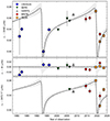 |
Fig. 5. Evolution of the main pulsation frequency ν1 (top) and ν2 (bottom) with a binary orbit fit (dashed line) according to Table 6 and the residuals to the fit (middle). The grey-shaded areas indicating the uncertainties. |
For a Keplerian orbit, the modulation of the intrinsic pulsation frequency γ can be computed for a given time t according to:
![Mathematical equation: $$ \begin{aligned} \nu = \gamma + K_{\nu } [\cos (\omega + \varphi _{(t,e,T,P)}) + e \cos \omega ], \end{aligned} $$](/articles/aa/full_html/2024/08/aa46942-23/aa46942-23-eq18.gif) (2)
(2)
with the modulation amplitude, Kν, the longitude of the periastron, ω, and the true anomaly, φ, which depends on t, the eccentricity, e, the periastron epoch, T, and the orbital period, P.
We again use UltraNest to fit Eq. (2) to the measurements of ν1 and find a highly significant solution for an eccentric orbit with a period of 27.14 ± 0.16 yr. The full solution is listed in Table 6 and the corresponding fit and its uncertainties are shown in Fig. 5.
Binary orbit solution.
If the binary interpretation is correct, the modulation of ν1 is not intrinsic to the primary star in the α Cir system (i.e. the roAp star) but due to the binary motions. Therefore, all pulsation frequencies should be affected in the same way as ν1. Consequently, a first mandatory test is to check if we can find a similar behaviour in the other pulsation frequencies. This is demonstrated in the bottom panel of Fig. 5 for ν2, where all observations follow the same trend as ν1 (reflected by the orbital fit) within about 3σ. Unfortunately, the graph is not as well populated as for ν1, which is due to the smaller amplitudes and therefore the inability to detect this frequency in all datasets.
The relative frequency change of ν1 translates into a radial velocity amplitude according to
 (3)
(3)
which results in 6.5 ± 1.9 km s−1 for α Cir. We can now calculate the mass function,
 (4)
(4)
as 0.035 ± 0.033 M⊙, where M1 and M2 are the mass of α CirA and its companion, respectively. Using a primary mass of 1.82 ± 0.11 M⊙ (Table 1) we can solve Eq. (4) for M2 as a function of the systems inclination i. This is illustrated in Fig. 6, showing that the mass of the companion ranges from some tenth to a few solar masses, depending on the inclination of the binary system. The mass estimate can further be used to determine the orbital separation a of the two stars:
 (5)
(5)
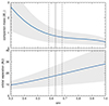 |
Fig. 6. Range of companion mass (top) and orbital separation (bottom) and their uncertainties (grey-shaded areas) for models as a function of the orbit inclination. The vertical lines indicate the inclination of the rotation axis of α Cir and its uncertainty. |
which is also given as a function of sin i in Fig. 6, showing that the system’s size is comparable to our outer solar system8.
In summary, we claim the detection of α Cir as a triple system, with the second companion orbiting α CirA in an eccentric orbit every about 27 yr.
The best way to test if α CirA is indeed orbited by a so far unknown companion is to search for the orbital signature in the already available radial velocity measurements of the system. Overall, α Cir is a quite bright star and has been spectroscopically studied for many decades. We were therefore confident to find historic RV measurement that spread out over (many years and in an ideal case), they would also cover the orbital phases where we can expect significant RV changes (> 10 km s−1) in a relatively short time (i.e. several months). In fact, plenty of spectroscopic studies from various observational sources can be found in the literature. However, most of them do not provide a value for the radial velocity and the actual spectroscopic observations are often too old to be included in modern online archives. We did also contact some of the principal authors, only to learn that this information is basically lost. The star is also listed in several catalogues that report RV measurements, but it has turned out that almost always the actual radial velocity listed in the catalogue originates from a single source obtained in 1911. However, we were able to collect a sample of nine individual RV measurements, which we briefly describe in the following:
The first RV measurement obtained of α Cir was carried out by Lunt (1918) with the Victoria telescope at the Royal Observatory, Cape of Good Hope, with six photographic plates obtained in mid-1911. CASPEC: Nine spectra obtained between Jun. 1985 and Apr. 1988 with the Cassegrain Echelle Spectrograph (CASPEC) at La Silla with the average RV given by Mathys et al. (1996). IUE: Five spectra obtained between October 1986 and October 1991 with the International Ultraviolet Explorer (IUE), which we downloaded from the MAST archive. The RV is determined by fitting the line centres of the MgII 2796.35 and 2803.53 Å and the MgI 2852.96 Å spectral lines. CES/UVES/UCLES: Six spectra obtained in Feb. 2001 with the Coude Echelle Spectrometer (CES) at La Silla observatory, one spectrum obtained in February 2002 with the Ultraviolet and Visual Echelle Spectrograph (UVES) at VLT, and five spectra obtained in May 2005 at the University College London Echelle Spectrograph (UCLES) at the Anglo-Australian Telescope. The RVs are extracted by fitting the NdIII 6145 Å spectral line and averaged afterwards. HARPS: Average RV of the 4800+ HARPS spectra obtained between Apr. 2005 and Feb. 2009 (see Sect. 3.5). FEROS: One spectrum obtained in Mar. 2014 with the Fiber-fed Extended Range Optical Spectrograph (FEROS) at La Silla. The RV is determined by fitting the core of the H-α spectral line. Gaia: RV listed in the Gaia DR2 catalogue of radial velocity standard stars (Soubiran et al. 2018). To the observational uncertainties we add 0.4 km s−1 (in quadrature) to account for the pulsation and rotation signal, which we determined from the HARPS data. Individual values are listed in Table 7.
Individual RV measurments with the mean epoch given in HJD.
The resulting radial velocities are illustrated in Fig. 7 as a function of the phase during the presumed 27.1-years binary orbit. The figure also shows the orbital fit from Fig. 5 scaled according to Eq. (3) and arbitrarily shifted by 0.23 km s−1 to align with the RV measurements. Even though the RV data do not cover the most sensitive orbital phases, it is quite obvious that they follow the same trend as we observed for the star’s pulsation frequencies. This is also supported by a linear fit to the RV data (except the one from Lunt 1918) that almost perfectly aligns with the orbital fit.
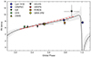 |
Fig. 7. Radial velocity measurements as a function of the orbital phase with the fit from Fig. 5 scaled according to Eq. (3) and vertically shifted by 0.23 km s−1. The red dashed-dotted line corresponds to a linear fit to the RV values (except the one from Lunt 1918). The horizontal error bars reflect the time range during which the RV is obtained. |
We consider this strong support for the ‘binary hypothesis’. An unambiguous confirmation, however, is only possible if one also covers the orbital phase near the periastron (around orbital phase equal to one in Fig. 7), where the radial velocity is supposed to change by more than 12 km s−1 in less than 16 months. Unfortunately, this phase only recently occurred somewhen between 2019 and 2020 – and will only happen again around 2047.
6. Rotation
The rotation period of α Cir was published by Kurtz et al. (1994) as Prot = 4.4790 ± 0.0001 d. Using spot modelling based on WIRE and the early BRITE and TESS data, Weiss et al. (2020) then improved Prot to 4.47930 ± 0.00002 d.
The orbital motion of α Cir should in principle also affect the rotation period determined by an external observer, as demonstrated in the previous section. However, since Prot is about 950 times longer than the main pulsation period, the resulting variation of the rotation period will be 950 times smaller than for the pulsation signal (see Eq. (3)). We can thus expect such an effect to be of the order of ±0.00005 d (or ±4 s). This is comparable to the uncertainties of the so far best determined rotation period and much smaller than the error of Prot when determined from the individual datasets. It is therefore inefficient to analyse the various datasets individually with, for instance, classical frequency analyses or even complex spot modelling.
A sensitive method to investigate the temporal stability of a periodic signal is based on a classical O − C approach (e.g. Breger & Pamyatnykh 1998). With a time base of almost eight years, the SMEI dataset provides a solid initial guess for Prot. We thus fit Eq. (1) to the SMEI data, but unlike for data preparation (Sect. 3), we let P be a free parameter in the fit and determine it to 4.47908 ± 0.00009 d. In a next step we used this to phase fold the individual datasets and fit a double harmonic function (Eq. (1)) with a fixed period to determine the phase of minimum light, ϕmin. If the star’s rotation period is constant and equal to the initial guess, the value of ϕmin would be the same for all datasets. If the initial guess slightly differs from the correct value, then ϕmin would linearly increase or decrease with time. If, however, the star’s rotation period is varying, for instance, due to evolutionary changes of the stellar radius or due to changes of the star’s angular momentum, ϕmin would parabolically change.
In fact, Fig. 8 shows that ϕmin increases with time and a parabolic fit ϕmin(t) = d + kt + βt2, with k = (1.04 ± 0.01)×10−5 and β = (− 1.0 ± 0.7)×10−10. This indicates that the increase is practically linear. The coefficient k of the linear term now allows us to correct the initial guess of the rotation frequency (νrot = 1/Prot), according to νrot, cor = νrot, initial − k, which gives a corrected rotation period of 4.4792890 ± 0.0000018 d, and which is smaller then the value mentioned by Holdsworth et al. (2021). The difference is 3σ according to the values given by the latter authors, but significantly more considering the small uncertainty, which is derived in the present paper. The fit procedure is repeated with the new Prot, which results in k = (6 ± 10)×10−8 and the same β as before. As a result, ϕmin(t) is now constant within the uncertainties (see the bottom panel of Fig. 8).
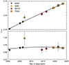 |
Fig. 8. Rotation phase of the light maxima with reference to our initial guess of Prot (4.47908 d, top) and the finally adopted value (4.4792890 d, bottom). Dashed lines indicate parabolic fits with the grey-shaded area giving the uncertainties. |
In Fig. 9, we show heavily binned versions of the various light curves, folded with the final rotation period along with the fits to measure the phase of minimum light. We note (especially for the TESS data) that the fits show small but significant systematic differences to the data. This is because the used model (Eq. (1)) basically represents a two-spot solution that underfits the data (see Weiss et al. 2020). This does, however, only marginally affect the determination of the phase of minimum light.
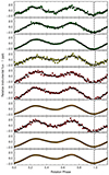 |
Fig. 9. Heavily binned light curves of α Cir folded with the finally adopted rotation period sorted by their observing epoch. Solid lines correspond to fits with Eq. (1) and the vertical dashed lines indicate the measured phase of the light minima. The datasets are sorted by their observing year and correspond from top to bottom to the WIRE 2000, 2005, and 2006 data, SMEI, BRITE 2014 and 2016 data, TESS 2019, BRITE 2021, TESS 2021, and the TESS 2023 data. |
7. Modulation of the pulsation signal
Over recent decades, there have been several attempts to interprete the variation of α Cir’s main pulsation frequency ν1 (e.g. Kurtz et al. 1993, 1994; Bruntt et al. 2009) but with inconclusive results. A problem so far was that the variation of the pulsation signal was studied by fitting the pulsation amplitude and phase in consecutive short subsets of the full light curve while holding the frequency fixed. This is insofar problematic as the frequency and phase are strongly correlated and keeping one of them fixed during the fit can easily distort the other. In fact, Bruntt et al. (2009) argued that while the pulsation amplitude is modulated by the rotation the phase is not, which needs to be proven.
Therefore, we followed a different approach. Instead of splitting the data into subsets in time, we split them into subsets in rotation phase. The individual subsets are thus similar in length (over time) as the full time series so that the original frequency resolution is approximately conserved allowing us to independently fit all parameters (frequency, amplitude, and phase) of ν1 in the subsets.
The results for the three TESS datasets are shown in Fig. 10 using ten equally sized bins in rotation phase. As was already found by Bruntt et al. (2009), the pulsation amplitude is rotationally modulated with its maximum almost coinciding with the phase of the light maxima of the rotational light variation (see panels a and b in Fig. 10). We further find that the amplitude modulation is quite stable over time, as it follows practically the same sinusoid in all three datasets. This is illustrated by the amplitude ratios relative to the 2019 data in panel c of Fig. 10, showing that the residuals relative to the amplitude change as a function of rotation phase (panel b of the same figure) is consistent with unity (within the uncertainties). Also, the frequency tends to follow some rotational modulation but the size is too small (well below 1nHz, see panel d of Fig. 10) to be considered significant.
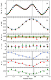 |
Fig. 10. Amplitude, frequency, and phase of the main pulsation frequency ν1 as a function of the rotation phase (zero point in time t0 = BJD 2 459 500.055) for the TESS 2019 (blue), 2021 (red), and 2023 (green) data. Panel a: heavily binned relative instrumental flux with the vertical dashed and dotted lines indicating the phase of the maximum and minimum light, respectively. Panel b: amplitude of the main pulsation signal (a1) in the various datasets. The black line gives a sinusoidal fit to the 2019 amplitudes with the vertical dashed line indicating the maximum amplitude. Panel c: amplitudes in the 2021 and 2023 data relative to the 2019 amplitudes. Coloured dashed lines and shaded areas give the average ratio and its standard deviation. Panel d: difference (in nHz) of the main pulsation frequency ν1 to the full-length dataset frequency νref (≡ν1 in Tables 3 and 4). Panels e, f, g: phase of the main pulsation signal Φ1. The black lines give the fits to observed values with the vertical dashed lines and grey-shaded areas indicating the minimum phases of the fits and their uncertainties, respectively. |
This is not the case for phase Φ1, which is clearly modulated with the rotation phase, Φrot, (see panels e to g of the same figure). Contrary to the pulsation amplitude, the phase modulation is not sinusoidal, but can be well approximated by a distorted sine,
 (6)
(6)
where x = 2π(Φrot + c) with a, b, and c are the fit parameters. While the amplitude of the phase modulation decreases with time from 8 ± 0.6 × 10⁻³ in 2019, to 6 ± 1 × 10⁻³ in 2021, to 4 ± 0.8 × 10⁻³ in 2023, the rotation phase of minimum pulsation phase is rather stable at about the same value as for the light maxima and maximum pulsation amplitude.
Similar phase modulations have been observed in roAp stars with dominant quadrupole mode oscillations (e.g. Holdsworth et al. 2016), however, to our knowledge, this has not yet been seen for dipole mode pulsators. This definitely deserves further attention in terms of the oblique pulsator model (e.g. Kurtz 1982). A detailed interpretation is beyond the scope of the present paper and we leave it to follow up studies.
However, the phase modulation (i.e. that it does not change by π, see, e.g. Kurtz et al. 1990) demonstrates that the pulsation node does not cross the line of sight, which is consistent with the mode geometry that follows from the amplitude distribution in the ν1 triplet. While the inequality of the sidelobe amplitudes result from the Coriolis force (Bigot & Dziembowski 2002), the ratio between the side and central peak amplitudes (Am) mostly arises from the rotational inclination (i) and the magnetic obliquity (β). For dipole modes, the relation is defined as:
 (7)
(7)
Using the observed values from Tables 1 and 3 gives β = 15.6 ± 1.6°. Therefore i + β < 90° indicating that only one magnetic pole is visible over the rotation cycle. In order to still give a double wave signature in the rotational light variation, the (majority) of the spots have to be on a single hemisphere, which is also indicated by photometric surface imaging (Weiss et al. 2020).
8. Discussion
The echelle diagram of the 2019 high-precision time series of TESS (Fig. 4) shows that the five rotationally split modes (ν1, ν2, ν3, ν6 and ν7) are most likely of three different degrees of l. Based on simulated amplitude modulations for an oblique pulsator model, Bruntt et al. (2009) argued that ν1 is very likely an axisymmetric dipole mode (l = 1, m = 0). From this, we can assume that, ν4, ν5, ν6, ν8, and ν10 are also dipole modes; ν2, ν3, ν11 are radial modes (see also Weiss et al. 2020); ν9 and ν12 are l = 2 modes; and ν7 is likely a l = 3 mode.
It could be argued that radial modes are usually not rotationally split. A possible explanation for the claimed splitting is, however, that the significantly inhomogeneous surface of α Cir modulates the pulsation amplitudes with the rotation period, so that radial modes are also split in the Fourier domain. Such phenomenon is known for other roAp stars and explained by the spotted pulsator model (Mathys 1985; Kurtz 1990) Another phenomenon (noted in Sect. 4.1) is the significantly curved dipole mode sequence in Fig. 4, contradicting theory (e.g. Tassoul 1980), which claims that high-radial order modes follow a straight line. This anomaly could be a consequence of the observed modes being distorted (e.g. Cunha 2006) by the strong magnetic field of α Cir (e.g. Mathys 2017).
Another peculiarity of α Cir is a systematic decrease of nearly all pulsation mode amplitudes between 2019 and 2021 by up to 10% and the highly significant frequency decrease during the same observing period. For the high-amplitude modes, we find on average a frequency shift of −21.8 ± 0.5 ppm. For ν1, this shift is even −55 ± 8 nHz. However, this trend is less obvious for the low-amplitude modes. Before the TESS and BRITE observations in 2021 became available we assumed that the change in ν1 is the signature of stellar evolution. In fact, Fig. 5 shows a statistically significant, almost linear increase of ν1 over time, when ignoring an outlier from literature (Kurtz et al. 1994). However, the new data from TESS and BRITE contradict clearly this simple view and call for a different explanation.
In Sect. 5 we argue that the main component of the already known visual binary system actually is a close binary. If we would see this system edge-on we could estimate from Fig. 5 that an eclipse should have been visible eventually between August 2019 and January 2020 (i.e. T + P from Table 6) during the last periastron of the system. Unfortunately, this is at least one months after the TESS 2019 observations ended, so that we cannot make any statement about an eclipsing system. It is, however, plausible to assume that the binary orbital axis is orientated roughly parallel to α CirA’s rotation axis, which can be estimated from the stars radius, the projected rotational velocity value, and the rotation period.
Using α Cir’s radius of 1.975 ± 0.03 R⊙ (from Table 1) gives an equatorial rotation velocity of 22.3 ± 0.3 km s−1 for the about 4.48 d rotation period. Since v sin i = 14 ± 1 km s−1 (Reiners & Schmitt 2003), sin i results in 0.63 ± 0.05 with a corresponding inclination of 39 ± 3°.
According to Fig. 6, the companion mass would then range somewhere between 0.4 and 1.6 M⊙. The high mass end of this range basically can be ruled out as it would make the two stars comparable in brightness (given the companion is not a neutron star) and the actual luminosity of α CirA would decrease to about 5 L⊙, which shifts the star below the zero-age main-sequence, considering the measured surface temperature. It is more plausible that the companion is a low-mass star, contributing only a small fraction to the total luminosity. A 0.4 M⊙ main sequence star has a luminosity of about 0.03 L⊙ therefore, it covers only about 0.3% of the systems total luminosity of about 10.5 L⊙. The spectral signature of this supposed companion has – to our knowledge – not yet been found, not even in high signal-to-noise spectroscopic measurements.
In Sect. 6, we demonstrate that the rotation phases of minimum light in the individual spot-modulated timeseries of α CirA can be used to improve the rotation period of α CirA. Indeed, the final value of Prot = 4.4792890 ± 0.0000018 d, which is consistent with the value determined by Weiss et al. (2020), but ten times more accurate.
9. Conclusion
Overall, α Cir has now been observed with improving accuracy from ground and space over more than 40 years, using spectrographs and photometers. The rotation period could be determined with an accuracy of ±0.4 ppm, which consequently represents one of the best known stellar rotation periods. Furthermore, α Cir has the richest frequency spectrum observed for any roAp stars, which promises spectacular insights about the structure and evolution of this group of peculiar stars.
In fact, the dominant pulsation period, ν1, changes with time, but, unexpectedly, the plausible first explanation that points to evolutionary effects is likely wrong. Instead, we propose the existence of a close companion. Obviously, new challenges have appeared due to higher precision of the data. The richness of the frequency spectrum, for instance, is foiled by phenomena not yet explained by theory, such as the curvature of a dipole mode sequence or unexplained amplitude changes.
We conclude that α Cir needs to remain on high-level observing programs, including attempts to confirm the close companion. In addition, a focus on the modelling of the internal structure of α Cir is required, considering in particular the effects of a magnetic field on the pulsation spectrum.
Each sector is about 27.4 days long and takes two satellite orbits.
Square root of the mean squared differences of consecutive data points.
Taken from the https://brite.camk.edu.pl/pub/index.html.
https://github.com/tkallinger/autoDFT on Github.
According to the convention established by Jeffreys (1998), the evidence for or against one of two hypotheses is considered ‘substantial’ for p ≳ 0.75, ‘strong’ for p ≳ 0.91, and ‘very strong’ for p ≳ 0.97.
The global evidence is a normalised logarithmic probability describing how well the model fits the data with respect to the uncertainties, parameter ranges, and the complexity of the fitted model.
Frequencies labeled with * or ** are presumably due to a modulation (see Table 3 caption).
Note that at α Cir’s distance of about 16.7 pc such a system has an apparent diameter of less than 0.05 milliarcseconds.
Acknowledgments
We gratefully thank Tanja Ryabchikova for providing us with radial velocity measurements from the CES, UVES, and UCLES spectra. We further thank Tim Bedding, Paul Shapshak, and Daniel Hey for useful comments on the manuscript. This paper includes data collected by the TESS mission, which are publicly available from the Mikulski Archive for Space Telescopes (MAST). Funding for the TESS mission is provided by NASA’s Science Mission directorate. Funding for the TESS Asteroseismic Science Operations Centre is provided by the Danish National Research Foundation (Grant agreement no.: DNRF106), ESA PRODEX (PEA 4000119301) and Stellar Astrophysics Centre (SAC) at Aarhus University. We thank the TESS team and staff and TASC/TASOC for their support of the present work. Furthermore, this paper is based on data collected by the BRITE Constellation satellite mission, designed, built, launched, operated and supported by the Austrian Research Promotion Agency (FFG), the University of Vienna, the Technical University of Graz, the Canadian Space Agency (CSA), the University of Toronto Institute for Aerospace Studies (UTIAS), the Foundation for Polish Science & Technology (FNiTP MNiSW), and National Science Centre (NCN).
References
- Aerts, C. 2021, Rev. Mod. Phys., 93, 015001 [Google Scholar]
- Baldry, I. K., Bedding, T. R., Viskum, M., Kjeldsen, H., & Frandsen, S. 1998, MNRAS, 295, 33 [NASA ADS] [CrossRef] [Google Scholar]
- Balmforth, N. J., Cunha, M. S., Dolez, N., Gough, D. O., & Vauclair, S. 2001, MNRAS, 323, 362 [NASA ADS] [CrossRef] [Google Scholar]
- Balona, L. A., & Laney, C. D. 2003, MNRAS, 344, 242 [NASA ADS] [CrossRef] [Google Scholar]
- Bigot, L., & Dziembowski, W. A. 2002, A&A, 391, 235 [NASA ADS] [CrossRef] [EDP Sciences] [Google Scholar]
- Bigot, L., & Kurtz, D. W. 2011, A&A, 536, A73 [NASA ADS] [CrossRef] [EDP Sciences] [Google Scholar]
- Breger, M., & Pamyatnykh, A. A. 1998, A&A, 332, 958 [NASA ADS] [Google Scholar]
- Bruntt, H., North, J. R., Cunha, M., et al. 2008, MNRAS, 386, 2039 [NASA ADS] [CrossRef] [Google Scholar]
- Bruntt, H., Kurtz, D. W., Cunha, M. S., et al. 2009, MNRAS, 396, 1189 [NASA ADS] [CrossRef] [Google Scholar]
- Buchner, J. 2016, Stat. Comput., 26, 383 [Google Scholar]
- Buzasi, D. 2002, in IAU Colloq. 185: Radial and Nonradial Pulsationsn as Probes of Stellar Physics, eds. C. Aerts, T. R. Bedding, & J. Christensen-Dalsgaard, ASP Conf. Ser., 259, 616 [NASA ADS] [Google Scholar]
- Cunha, M. S. 2006, MNRAS, 365, 153 [NASA ADS] [CrossRef] [Google Scholar]
- Cunha, M. S., Alentiev, D., Brandão, I. M., & Perraut, K. 2013, MNRAS, 436, 1639 [NASA ADS] [CrossRef] [Google Scholar]
- Deal, M., Cunha, M. S., Keszthelyi, Z., Perraut, K., & Holdsworth, D. L. 2021, A&A, 650, A125 [NASA ADS] [CrossRef] [EDP Sciences] [Google Scholar]
- Feroz, F., Hobson, M. P., & Bridges, M. 2009, MNRAS, 398, 1601 [NASA ADS] [CrossRef] [Google Scholar]
- Gough, D. 1985, Nature, 314, 14 [NASA ADS] [CrossRef] [Google Scholar]
- Holdsworth, D. L., Kurtz, D. W., Smalley, B., et al. 2016, MNRAS, 462, 876 [NASA ADS] [CrossRef] [Google Scholar]
- Holdsworth, D. L., Cunha, M. S., Kurtz, D. W., et al. 2021, MNRAS, 506, 1073 [NASA ADS] [CrossRef] [Google Scholar]
- Huber, D., White, T. R., Metcalfe, T. S., et al. 2022, AJ, 163, 79 [NASA ADS] [CrossRef] [Google Scholar]
- Husser, T. O., Wende-von Berg, S., Dreizler, S., et al. 2013, A&A, 553, A6 [NASA ADS] [CrossRef] [EDP Sciences] [Google Scholar]
- Jackson, B. V., Buffington, A., Hick, P. P., et al. 2004, Sol. Phys., 225, 177 [NASA ADS] [CrossRef] [Google Scholar]
- Jeffreys, H. 1998, Theory of Probability, Oxford Classic Texts in the Physical Sciences (New York: The Clarendon Press, Oxford University Press) [Google Scholar]
- Jenkins, J. M., Twicken, J. D., McCauliff, S., et al. 2016, in Software and Cyberinfrastructure for Astronomy IV, eds. G. Chiozzi, & J. C. Guzman, SPIE Conf. Ser., 9913, 99133E [Google Scholar]
- Kallinger, T., & Weiss, W. W. 2017, in Second BRITE-Constellation Science Conference: Small Satellites - Big Science, eds. K. Zwintz, & E. Poretti, 5, 113 [NASA ADS] [Google Scholar]
- Kallinger, T., Weiss, W. W., Beck, P. G., et al. 2017, A&A, 603, A13 [NASA ADS] [CrossRef] [EDP Sciences] [Google Scholar]
- Kochukhov, O., & Ryabchikova, T. 2001, A&A, 377, L22 [NASA ADS] [CrossRef] [EDP Sciences] [Google Scholar]
- Kochukhov, O., Shulyak, D., & Ryabchikova, T. 2009, A&A, 499, 851 [NASA ADS] [CrossRef] [EDP Sciences] [Google Scholar]
- Kurtz, D. W. 1982, MNRAS, 200, 807 [NASA ADS] [CrossRef] [Google Scholar]
- Kurtz, D. W. 1990, ARA&A, 28, 607 [NASA ADS] [CrossRef] [Google Scholar]
- Kurtz, D. 2022, Annual Conference and General Assembly of the African Astronomical Society, held 14-18 March, 2022 (AfAS-2022) [Google Scholar]
- Kurtz, D. W., & Balona, L. A. 1984, MNRAS, 210, 779 [NASA ADS] [CrossRef] [Google Scholar]
- Kurtz, D. W., & Cropper, M. S. 1981, Inf Bull. Var. Stars, 1987, 1 [Google Scholar]
- Kurtz, D. W., & Holdsworth, D. L. 2020, in Dynamics of the Sun and Stars; Honoring the Life and Work of Michael J. Thompson, eds. M. J. P. F. G. Monteiro, R. A. García, J. Christensen-Dalsgaard, & S. W. McIntosh, ASS Proc., 57, 313 [NASA ADS] [CrossRef] [Google Scholar]
- Kurtz, D. W., Shibahashi, H., Goode, P. R., et al. 1990, MNRAS, 247, 558 [NASA ADS] [Google Scholar]
- Kurtz, D. W., Martinez, P., & Ashley, R. P. 1993, MNRAS, 264, 529 [NASA ADS] [CrossRef] [Google Scholar]
- Kurtz, D. W., Sullivan, D. J., Martinez, P., & Tripe, P. 1994, MNRAS, 270, 674 [NASA ADS] [Google Scholar]
- Lenz, P., & Breger, M. 2005, Commun. Asteroseismol., 146, 53 [Google Scholar]
- Lunt, J. 1918, ApJ, 48, 261 [NASA ADS] [CrossRef] [Google Scholar]
- Mathys, G. 1985, A&A, 151, 315 [NASA ADS] [Google Scholar]
- Mathys, G. 2017, A&A, 601, A14 [NASA ADS] [CrossRef] [EDP Sciences] [Google Scholar]
- Mathys, G., Kharchenko, N., & Hubrig, S. 1996, A&A, 311, 901 [NASA ADS] [Google Scholar]
- Mermilliod, J. C. 2006, VizieR Online Data Catalog, II/168 [Google Scholar]
- Mkrtichian, D. E., & Hatzes, A. P. 2013, in Progress in Physics of the Sun and Stars: A New Era in Helio- and Asteroseismology, eds. H. Shibahashi, & A. E. Lynas-Gray, ASP Conf. Ser., 479, 115 [NASA ADS] [Google Scholar]
- Monier, R. 2020, Res. Notes Am. Astron. Soc., 4, 160 [NASA ADS] [Google Scholar]
- Pablo, H., Whittaker, G. N., Popowicz, A., et al. 2016, PASP, 128, 125001 [Google Scholar]
- Paunzen, E. 2015, A&A, 580, A23 [NASA ADS] [CrossRef] [EDP Sciences] [Google Scholar]
- Popowicz, A., Pigulski, A., Bernacki, K., et al. 2017, A&A, 605, A26 [NASA ADS] [CrossRef] [EDP Sciences] [Google Scholar]
- Reiners, A., & Schmitt, J. H. M. M. 2003, A&A, 412, 813 [NASA ADS] [CrossRef] [EDP Sciences] [Google Scholar]
- Ricker, G. R., Winn, J. N., Vanderspek, R., et al. 2015, J. Astron. Telesc. Instrum. Syst., 1, 014003 [Google Scholar]
- Schneider, H., & Weiss, W. W. 1983, Inf. Bull. Var. Stars, 2306, 1 [NASA ADS] [Google Scholar]
- Schneider, H., & Weiss, W. W. 1989, A&A, 210, 147 [NASA ADS] [Google Scholar]
- Shibahashi, H., & Saio, H. 1985, PASJ, 37, 601 [NASA ADS] [Google Scholar]
- Sinachopoulos, D. 1989, A&AS, 81, 103 [NASA ADS] [Google Scholar]
- Soubiran, C., Jasniewicz, G., Chemin, L., et al. 2018, A&A, 616, A7 [NASA ADS] [CrossRef] [EDP Sciences] [Google Scholar]
- Stassun, K. G., & Torres, G. 2016, AJ, 152, 180 [Google Scholar]
- Stassun, K. G., & Torres, G. 2021, ApJ, 907, L33 [NASA ADS] [CrossRef] [Google Scholar]
- Stassun, K. G., Collins, K. A., & Gaudi, B. S. 2017, AJ, 153, 136 [Google Scholar]
- Stassun, K. G., Corsaro, E., Pepper, J. A., & Gaudi, B. S. 2018, AJ, 155, 22 [Google Scholar]
- Tarrant, N. J., Chaplin, W. J., Elsworth, Y., Spreckley, S. A., & Stevens, I. R. 2008, A&A, 483, L43 [NASA ADS] [CrossRef] [EDP Sciences] [Google Scholar]
- Tassoul, M. 1980, ApJS, 43, 469 [Google Scholar]
- Torres, G., Andersen, J., & Giménez, A. 2010, A&A Rev., 18, 67 [Google Scholar]
- Trifonov, T., Tal-Or, L., Zechmeister, M., et al. 2020, VizieR Online Data Catalog, J/A+A/636/A74 [Google Scholar]
- Weiss, W. W., & Schneider, H. 1984, A&A, 135, 148 [NASA ADS] [Google Scholar]
- Weiss, W. W., Jenkner, H., & Wood, H. J. 1976, IAU Colloq. 32: Physics of Ap Stars [Google Scholar]
- Weiss, W. W., Moffat, A. F. J., Schwarzenberg-Czerny, A., et al. 2014, in Precision Asteroseismology, Proceedings of the International Astronomical Union, eds. J. A. Guzik, W. J. Chaplin, G. Handler, & A. Pigulski, IAU S301, 9, 67 [Google Scholar]
- Weiss, W. W., Fröhlich, H. E., Pigulski, A., et al. 2016, A&A, 588, A54 [NASA ADS] [CrossRef] [EDP Sciences] [Google Scholar]
- Weiss, W. W., Fröhlich, H. E., Kallinger, T., et al. 2020, A&A, 642, A64 [NASA ADS] [CrossRef] [EDP Sciences] [Google Scholar]
All Tables
Significant pulsation frequencies in the WIRE, BRITE, and HARPS observations derived in the present analysis and completed by literature values.
All Figures
|
Fig. 1. Spectral energy distribution of α Cir. Red symbols represent the observed photometric measurements, where the horizontal bars represent the effective width of the passband. Blue symbols are the model fluxes from the best-fit PHOENIX atmosphere model (black). The Gaia spectrum is shown overlaid as a gray swathe (also shown in the inset plot). |
| In the text | |
|
Fig. 2. TESS 2019 (left), 2021 (middle), and 2023 (right) light curves. Panels a: double harmonic fit (blue lines) to the original PDC_SAP data (grey dots). Panels b: original (grey dots) and heavily smoothed (red lines) residuals to the double harmonic fit of panels a. Panels c: original data corrected for the smoothed residuals from panels b (grey dots – these data are used for the rotation analysis) along with a double harmonic fit (blue lines). Panels d: original (grey dots) and heavily smoothed residuals (red lines) from panels c. Panels e: residuals from panels d. These data are used for the pulsation analysis. |
| In the text | |
|
Fig. 3. Fourier amplitude spetra of the TESS 2019, WIRE 2006, combined BRITE 2014-16 light curves, and the HARPS radial velocities with the significant TESS frequencies overlaid as vertical red dotted lines. The original spectra are shown in the left panels, whereas right panels give the spectra after prewhitening the one to three most significant frequencies. |
| In the text | |
|
Fig. 4. Echelle diagram of the TESS 2019 frequencies with the (blue) symbol size indicating the mode amplitude and the annotation according to Table 3. Red and green symbols give the corresponding frequencies in the 2021 and 2023 dataset, respectively. Modes of presumably the same spherical degree are connected by dashed line segments. |
| In the text | |
|
Fig. 5. Evolution of the main pulsation frequency ν1 (top) and ν2 (bottom) with a binary orbit fit (dashed line) according to Table 6 and the residuals to the fit (middle). The grey-shaded areas indicating the uncertainties. |
| In the text | |
|
Fig. 6. Range of companion mass (top) and orbital separation (bottom) and their uncertainties (grey-shaded areas) for models as a function of the orbit inclination. The vertical lines indicate the inclination of the rotation axis of α Cir and its uncertainty. |
| In the text | |
|
Fig. 7. Radial velocity measurements as a function of the orbital phase with the fit from Fig. 5 scaled according to Eq. (3) and vertically shifted by 0.23 km s−1. The red dashed-dotted line corresponds to a linear fit to the RV values (except the one from Lunt 1918). The horizontal error bars reflect the time range during which the RV is obtained. |
| In the text | |
|
Fig. 8. Rotation phase of the light maxima with reference to our initial guess of Prot (4.47908 d, top) and the finally adopted value (4.4792890 d, bottom). Dashed lines indicate parabolic fits with the grey-shaded area giving the uncertainties. |
| In the text | |
|
Fig. 9. Heavily binned light curves of α Cir folded with the finally adopted rotation period sorted by their observing epoch. Solid lines correspond to fits with Eq. (1) and the vertical dashed lines indicate the measured phase of the light minima. The datasets are sorted by their observing year and correspond from top to bottom to the WIRE 2000, 2005, and 2006 data, SMEI, BRITE 2014 and 2016 data, TESS 2019, BRITE 2021, TESS 2021, and the TESS 2023 data. |
| In the text | |
|
Fig. 10. Amplitude, frequency, and phase of the main pulsation frequency ν1 as a function of the rotation phase (zero point in time t0 = BJD 2 459 500.055) for the TESS 2019 (blue), 2021 (red), and 2023 (green) data. Panel a: heavily binned relative instrumental flux with the vertical dashed and dotted lines indicating the phase of the maximum and minimum light, respectively. Panel b: amplitude of the main pulsation signal (a1) in the various datasets. The black line gives a sinusoidal fit to the 2019 amplitudes with the vertical dashed line indicating the maximum amplitude. Panel c: amplitudes in the 2021 and 2023 data relative to the 2019 amplitudes. Coloured dashed lines and shaded areas give the average ratio and its standard deviation. Panel d: difference (in nHz) of the main pulsation frequency ν1 to the full-length dataset frequency νref (≡ν1 in Tables 3 and 4). Panels e, f, g: phase of the main pulsation signal Φ1. The black lines give the fits to observed values with the vertical dashed lines and grey-shaded areas indicating the minimum phases of the fits and their uncertainties, respectively. |
| In the text | |
Current usage metrics show cumulative count of Article Views (full-text article views including HTML views, PDF and ePub downloads, according to the available data) and Abstracts Views on Vision4Press platform.
Data correspond to usage on the plateform after 2015. The current usage metrics is available 48-96 hours after online publication and is updated daily on week days.
Initial download of the metrics may take a while.