| Issue |
A&A
Volume 687, July 2024
|
|
|---|---|---|
| Article Number | A94 | |
| Number of page(s) | 10 | |
| Section | Catalogs and data | |
| DOI | https://doi.org/10.1051/0004-6361/202449560 | |
| Published online | 02 July 2024 | |
High-precision astrometry with VVV
II. A near-infrared extension of Gaia into the Galactic plane★
1
INAF – Osservatorio Astronomico di Padova,
Vicolo dell’Osservatorio 5,
Padova
35122, Italy
e-mail: massimo.griggio@inaf.it
2
Dipartimento di Fisica, Università di Ferrara,
Via Giuseppe Saragat 1,
Ferrara
44122, Italy
3
Space Telescope Science Institute,
3700 San Martin Drive,
Baltimore, MD
21218, USA
4
AURA for the European Space Agency, Space Telescope Science Institute,
3700 San Martin Drive,
Baltimore, MD
21218, USA
5
Institute of Astronomy, University of Cambridge,
Madingley Rd,
Cambridge
CB3 0HA, UK
6
Institute of Astrophysics, Universidad Andres Bello,
Fernandez Concha 700, Las Condes,
Santiago, Chile
7
Vatican Observatory,
V00120
Vatican City State, Italy
8
Departamento de Física, Universidade Federal de Santa Catarina,
Trindade
88040-900,
Florianópolis, Brazil
Received:
9
February
2024
Accepted:
18
March
2024
Aims. We use near-infrared, ground-based data from the VISTA Variables in the Via Lactea (VVV) survey to indirectly extend the astrometry provided by the Gaia catalog to objects in heavily extinct regions toward the Galactic bulge and plane that are beyond Gaia’s reach.
Methods. We made use of state-of-the-art techniques developed for high-precision astrometry and photometry with the Hubble Space Telescope to process the VVV data. We employed empirical, spatially variable, effective point spread functions and local transformations to mitigate the effects of systematic errors, like residual geometric distortion and image motion, and to improve measurements in crowded fields and for faint stars. We also anchored our astrometry to the absolute reference frame of Gaia Data Release 3.
Results. We measure between 20 and 60 times more sources than Gaia in the region surrounding the Galactic center, obtaining a single-exposure precision of about 12 mas and a proper-motion precision of better than 1 mas yr−1 for bright, unsaturated sources. Our astrometry provides an extension of Gaia into the Galactic center. We publicly release the astro-photometric catalogs of the two VVV fields considered in this work, which contain a total of ~3.5 million sources. Our catalogs cover ~3 sq. deg, about 0.5% of the entire VVV survey area.
Key words: astrometry / parallaxes / proper motions
The catalog is available at the CDS via anonymous ftp to cdsarc.cds.unistra.fr (130.79.128.5) or via https://cdsarc.cds.unistra.fr/viz-bin/cat/J/A+A/687/A94
© The Authors 2024
 Open Access article, published by EDP Sciences, under the terms of the Creative Commons Attribution License (https://creativecommons.org/licenses/by/4.0), which permits unrestricted use, distribution, and reproduction in any medium, provided the original work is properly cited.
This article is published in open access under the Subscribe to Open model. Subscribe to A&A to support open access publication.
1 Introduction
The Gaia mission (Gaia Collaboration 2016) has revitalized many scientific research fields by providing the community with exquisite astrometry and photometry for more than a billion sources. All-sky coverage and astrometric accuracy and precision also make the Gaia catalogs among the best resources for technical projects like catalog and image registration in the International Celestial Reference System. The Gaia mission in fact provides an absolute astrometric reference frame on the sky, which can be used to derive geometric-distortion corrections for many cameras, as is shown by, for example, Griggio et al. (2022).
However, Gaia suffers from a few shortcomings, one of which is that it is highly incomplete even for bright sources in high-density fields, such as in the proximity of globular clusters or the Galactic bulge (Fabricius et al. 2021). In addition, the Gaia catalog contains only sources brighter than G ~ 21, which greatly limits its effectiveness in dust-enshrouded regions, such as those toward the Galactic plane. For these reasons, Gaia has limited applications for scientific or technical programs requiring high-precision astrometry for reddened bulge and disk objects.
The Galactic bulge is the ideal laboratory in which to study stellar interactions in high-density environments on galactic scales, providing insights into the early history of the Milky Way (e.g., Barbuy et al. 2018; Zoccali 2019; Fragkoudi et al. 2020), and astrometry represents a valuable tool with which to investigate the stellar populations in the bulge. In particular, proper motions allow us to separate bulge and disk stars and to identify gravitationally bound systems such as comoving groups, star clusters, and stellar streams (e.g., Garro et al. 2022b; Kader et al. 2022). Moreover, the Galactic bulge is where most of the microlensing events have been discovered – given the high density of sources in the bulge – and precise astrometry plays a fundamental role in the determination of the geometry of the event and of the masses of the involved bodies (Mróz et al. 2019). Proper motion measurements have also been essential for studies of new and old globular clusters in the Milky Way (Minniti et al. 2017, 2021a; Contreras Ramos et al. 2018; Garro et al. 2020, 2022a), and the accurate measurement of proper motions is key to identifying old globular clusters in the vicinity of the Galactic center and measuring their orbital properties (Minniti et al. 2021b, 2024).
The VISTA Variables in the Via Lactea (VVV, Minniti et al. 2010) is a near-infrared survey of the Galactic bulge and most of the disk obtained with the wide-field camera mounted at the Visible and Infrared Survey Telescope for Astronomy (VISTA, located at the Paranal Observatory in Chile). The VVV survey covers ~528 sq. deg of some of the most complex regions of the Milky Way in terms of high extinction and crowding. Its extension, VVVx (Minniti 2018), reobserved the same regions covered by its predecessor, and observed for the first time new areas that were not included in the original VVV plan. The combination of VVV and VVVx data provides an incredible dataset covering about 1700 sq. deg observed between 20 and 300 times, with a temporal baseline of up to ten years.
The VVV survey is carried out with a near-infrared, wide-field imager, the VIsta InfraRed CAMera (VIRCAM). VIRCAM is an array of 16 Raytheon VIRGO Mercury Cadmium Telluride 2048 × 2048-pixels detectors, arranged in a 4 × 4 grid. The gaps between the VIRCAM detectors are 42.5 and 90% of the detector’s size in the x and y directions, respectively. This layout allows VIRCAM to cover a field of view of 0.6 deg2 in a single pointing (a “pawprint”, following the official nomenclature). The VVV survey observed a given patch of sky (a “tile”) with a 3 × 2 mosaic, covering about 1.4 × 1.1 deg2 without gaps. The Cambridge Astronomical Survey Unit (CASU) is responsible for the data reduction, catalog generation, and calibration of both photometry and astrometry (Irwin et al. 2004; Lewis et al. 2010). The survey lasted five years, from 2010 to 2015, and observed the disk and bulge between 50 and 80 times in the KS filter. Additionally, two epochs in Z, Y, J, and H filters were acquired at the beginning and end of the survey. The VVV and VVVx surveys were mainly designed for photometric variability studies, but their multi-epoch strategy also enables astrometric analyses, as has been demonstrated by, for example, Libralato et al. (2015) and Smith et al. (2018).
Libralato et al. (2015, hereafter Paper I) presented a new pipeline to process the VIRCAM data. They used a calibration field centered on the globular cluster NGC 5139 to derive a new geometric distortion (GD) solution for the VIRCAM detector, which enables high-precision astrometry with the VVV data. They reprocessed the data of the VVV tile containing the globular cluster NGC 6656 and derived proper motions with a precision of ~1.4 mas yr−1, using 45 epochs over a time baseline of four years.
Smith et al. (2018) presented an astrometric catalog (VIRAC) of proper motions and parallaxes for the entire VVV area based on the CASU pipeline data; this catalog contains 312 million sources with proper motions and 6935 sources with parallaxes, and currently represents the largest astrometric catalog derived from VVV. Their proper motions achieve a precision of better than 1 mas yr−1 for bright sources, and a few mas yr−1 at KS = 16. However, their astrometry is not absolute, as they did not have at the time the Gaia all-sky reference frame to anchor their positions. Moreover, uncertainties on the relative to absolute proper motion calibration limit the accuracy of investigations on large Galactic scales.
In this paper, we use the VVV data (not VVVx) to extend the Gaia astrometry to reddened sources in the Galactic plane. In Fig. 1 we show the coverage of the VVV survey in Galactic coordinates, superimposed on a source-density map of the Gaia Data Release 3 (DR3, Gaia Collaboration 2023) catalog. We highlight in light blue the two tiles considered in this work; namely, b248 (South-East of the Galactic center) and b333 (which contains the Galactic center). The density map shows that the number of sources accessible to Gaia in the Galactic plane is limited by dust and crowding. As was anticipated, this limit makes certain investigations unfeasible in this region, and it is the primary motivation behind our work. We chose these two fields to test our methods in two environments with very different densities of Gaia sources: tile b248 has about 350 Gaia sources per sq. arcmin, whereas tile b333 has an average of 25 sources per sq. arcmin. As in Paper I, we used spatially variable empirical, effective point spread functions (ePSFs; see e.g., Anderson et al. 2006) to precisely measure the positions and fluxes of all of the sources in any given VVV image, and adopted local transformations (Anderson et al. 2006) to collate multiple singleimage astro-photometric catalogs, to minimize systematic errors such as residual GD and atmospheric effects, and to achieve the best astrometric precision possible. In addition, we significantly improve over previous efforts by: (i) employing a combination of first- and second-pass photometric stages specifically designed to improve measurements in crowded fields and for faint stars; and (ii) linking our astrometry to that of the Gaia DR3 catalog, as is done in, for example, Bedin & Fontanive (2018, 2020) and Libralato et al. (2021).
The paper is organized as follows. In Sect. 2 we describe the data reduction process, the construction of the master frame by leveraging the Gaia DR3 catalog, and the photometric registration. Section 3 provides an overview of the proper motions fit procedure. Section 4 shows the consistency of our catalog with respect to Gaia. In Sect. 5, we compare our results with the current public release of the VIRAC catalog (version 1) and show the improvements enabled by our method. In Sect. 6, we present an application of our new data reduction by measuring the parallax of a sample of sources, and compare them with those in the Gaia catalog. Finally, in Sect. 7 we outline our data reduction strategy and in Sect. 8 we conclude the paper with a summary of our work.
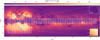 |
Fig. 1 Gaia DR3 source density around the region covered by the VVV survey. White boxes represent VVV tiles. We highlight in light blue the two tiles considered in this work; namely, b333 in the Galactic center and b248 on the southern bulge. Density map data were taken from the Gaia archive. |
2 Data reduction
In the first stage of the data reduction – that is, “preliminary photometry”, – we focused on the bright, unsaturated members. These sources were used to define the master frame by crossmatching their positions with those measured by Gaia. Preliminary photometry was obtained as is described in Paper I. We started with the pre-reduced images downloaded from the CASU archive and we treated each of the sixteen detectors separately. Our preprocessing routine is responsible for applying a series of cleaning algorithms to flag cosmic rays and mask bad pixels and saturated stars.
For each detector, we derived a 5 × 5 array of ePSFs using bright, isolated, and unsaturated sources, as was described by Anderson et al. (2006). We used these ePSF models to measure the positions and fluxes of the sources in each image. Our preliminary photometric catalogs contain positions, instrumental magnitudes defined as −2.5 · log(flux), and a parameter called quality-of-fit (QFIT), which represents the goodness of the ePSF-model fit for each star (see, e.g., Anderson et al. 2008a). A QFIT value close to 0 represents a good ePSF fit. In our VVV catalogs, bright and isolated sources typically have QFIT < 0.15. Bright, unsaturated stars close to saturation (with instrumental magnitudes between approximately −13.5 and −12, depending on the detector) show higher (>0.2) QFIT values. These sources appear to also exhibit inaccuracies in their flux measurements in the VIRAC catalog (see Fig. 10). What causes these bright stars, which should have a QFIT close to 0, to behave differently from the other bright, unsaturated sources is unclear. Nevertheless, we treated them as saturated and excluded the centermost pixels from the ePSF fitting to improve their photometry and astrometry. The threshold used to identify these objects was empirically defined for each detector.
The calibration of the GD cannot be performed via auto-calibration techniques with the VVV data, as the dither pattern is not suited for this purpose (see, e.g., Libralato et al. 2014; Häberle et al. 2021). We attempted to derive the GD solution by exploiting the Gaia DR3 catalog, following the procedure described in Griggio et al. (2022, 2023). However, given the short exposure time of the VVV images (~4 s), we were ultimately limited by the atmospheric image motion. In fact, the minimum exposure time needed to mitigate the impact of large-scale semi-periodic and correlated atmospheric noise, which can adversely affect ground-based astrometry, is approximately 30 s, as was determined by, for example, Platais et al. (2002, 2006), or Libralato et al. (2014). To show the effect of image motion, we cross-identified the stars in the astro-photometric catalogs of a set of consecutive VVV images and in the Gaia DR3 catalog. Gaia positions were propagated at the epoch of the VVV images by means of the Gaia DR3 proper motions and projected on the tangent plane of each VVV exposure. We then used six-parameter linear transformations to transform the GD-corrected positions in each VVV frame onto the Gaia reference frame system. Figure 2 shows the positional residuals generated by this comparison for a set of consecutive VVV images. Even though these images were taken within less than one minute, the residuals show different trends. Computing the GD solution from these images results in a null mean correction, as the random residuals due to image motion cancel out. For this reason, it is not possible to improve the GD solution derived in Paper I using the VVV data itself.
We then corrected the VVV raw positions with the GD solution of Paper I, which we consider more reliable as it was computed from well-exposed images of a calibration field specifically observed to calibrate the GD. We will explain later, in Sect. 2.4, how we mitigated the effect of image motion.
Besides the GD, we also needed to consider projection effects resulting from the large dithers of the images and the wide field of view of VIRCAM (see discussion in Paper I). As a result, images lie in different tangent planes, and we need to account for this as is done in, for example, Griggio et al. (2022). To do so, after correcting the raw positions with the GD solution, we used the information contained in the fits header of each image to project the detector-based coordinates onto equatorial coordinates, as in Bedin & Fontanive (2018), adopting a pixel scale of 0.339 arcsec px−1 (Paper I). We then projected all positions from all catalogs back into a common plane, using as a tangent point the average pointing position of all the images of the same tile. After this procedure, all single-exposure catalogs lie on the same tangent plane.
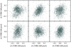 |
Fig. 2 Positional residuals obtained by crossmatching the catalogs of a set of consecutive images with Gaia after the GD solution derived with the VVV dataset was applied. Each panel corresponds to a distinct image. The residuals display different trends, preventing a precision of less than ~0.1 pixels (~35 mas) in a single exposure with this approach. |
2.1 The master frame
A key step toward our goal is the construction of a common reference frame, hereafter “master frame”, in which we can combine our images. Thanks to the Gaia mission, we already have an all-sky, absolute reference frame to which we can anchor our astrometry. We used the Gaia DR3 catalog to define the master frame as follows:
We propagated the Gaia positions to the corresponding epoch of each VVV pawprint set using Gaia proper motions.
We projected these adjusted positions onto the same tangent plane adopted for the tile.
We crossmatched the sources in each single-exposure catalog with those in the Gaia DR3 catalog, and derived the coefficients of the six-parameters linear transformations that bring the image-based coordinates onto the Gaia absolute reference frame.
2.2 Photometric registration
We registered the photometry to the 2MASS photometric system (Skrutskie et al. 2006) using the Gaia-2MASS crossmatched table available in the Gaia archive. We selected the best measured sources in both our catalogs and 2MASS, and used these sources to calculate the photometric zero points to transform the instrumental magnitudes measured in each single image into the 2MASS photometric system.
The 2MASS filter passbands are slightly different from those of the VISTA filters, and a more precise calibration would need to account for several factors, as is described in Gonzalez-Fernandez et al. (2018) and Hajdu et al. (2020). However, since in this work we are focused on obtaining high-precision astrometry, we neglected second-order corrections. In fact, the largest term in the photometric-calibration equation between the 2MASS and VISTA magnitudes is the color term, and it is on the order of a few hundredths of magnitudes at most. As such, the correction introduced by this term would be very small. Nonetheless, we plan to perform a more accurate calibration in the next releases, including airmass, extinction, and color terms.
2.3 Second-pass photometry
The “second-pass” photometry was performed using a version of the software KS2 (an evolution of the code presented in Anderson et al. 2008b, developed for the Hubble Space Telescope), opportunely modified to work with VIRCAM images, and adapted to wide-field imagers by Griggio et al. (2022, 2023). The software is designed to obtain deep photometry in crowded fields, by iterating a find-measure-subtract routine that employs all images simultaneously to improve the detection of faint sources. A description of KS2 can be found in, for example, Bellini et al. (2017) and Scalco et al. (2021). Briefly, the flux was measured by fitting the ePSF to the inner 5 × 5 pixels of the source after subtracting the local sky, using the appropriate ePSF for each image, and then averaging out between all the exposures. Stars measured in the previous iteration were subtracted from the image at each step. The second-pass photometry was carried out separately for each epoch in the KS filter: we considered as an epoch each set of images taken on the same day. A list of stars (derived from the preliminary photometry) was given as an input to the routine, and it was used to construct a weighted mask around bright sources, which helped to avoid PSF-related artifacts. In addition to the averaged master frame positions, the KS2 software outputs a file that contains, for each source, the raw position and neighbor-subtracted flux as measured in every single exposure. In addition to positions and fluxes, KS2 also outputs a few diagnostic parameters (see, e.g., Bedin et al. 2009), that can be used to reject poorly measured sources and detector artifacts, or to identify galaxies. In addition to the KS exposures, we also performed the second-pass photometry on all the J images of each tile, which we used only to build the color-magnitude diagrams. The color-magnitude diagrams of the two tiles analyzed in this work are shown in Fig. 3. The nonphysical drop in the number of sources around KS ~ 12 is due to our quality cut in the QFIT parameter: at this magnitude level there is a transition between unsaturated and saturated sources, and it is here where most of the stars showing unexpectedly high QFIT values lie, as is discussed in Sect. 2. Some of these problematic sources end up being measured as unsaturated as the thresholds that we set to identify these objects are not perfect, resulting in an overall high QFIT value.
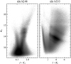 |
Fig. 3 Color-magnitude diagrams for tiles b248 (left) and b333 (right); see the text for details. |
2.4 The boresight correction
Image motion imposes a severe limitation on the astrometric precision achievable with VVV data. Indeed, it leads to local systematic position errors whose pattern changes even between subsequent exposures, up to ~0.15 pixels (~50 mas, see Fig. 2). This is far more than the single-measurement astrometric precision enabled by the GD solution, which has been shown to reach ~8 mas (Paper I). We employed a local mitigation to the effects of image motion on a given source (the target source) through a so-called “boresight” correction (see, e.g., Anderson & van der Marel 2010; Bedin et al. 2014). Our correction leverages the Gaia catalog, as it provides a sufficient number of reference Gaia sources even in regions toward the Galactic center. The number of neighboring reference sources for the correction is a compromise between the need for high statistics and for the correction to be as local as possible, even in regions where the Gaia source density is low. We achieved this by requiring at least 15 reference sources within a circular region of radius at most 300 pixels (and at least 50 pixels) from the target source.
For each epoch, we calculated the mean position of each source as follows:
We applied the GD correction to the raw positions of the sources in each image.
We projected the corrected positions onto the sky, and then we projected them back onto the common tangent plane of the tile.
Using well-measured sources in common with Gaia (excluding the target), we computed the transformations to bring the positions from the tangent plane to the master frame.
For each target star, we selected the neighboring sources in common with Gaia in each image, and we calculated the residuals between their positions transformed into the master frame and those given by Gaia (again, excluding the target star). The mean residual gives the boresight correction for each target source of each image.
We then transformed the positions of the target star as measured in the single images into the master frame, and applied to these values their boresight correction.
Finally, we calculated the average position, to which we associate the error on the mean as an estimate of the uncertainty.
Figure 4 is similar to Fig. 2, but with the positional residuals computed after the image-motion correction was applied. It is clear that the distribution of the residuals is much tighter than before, with a dispersion of about 12 mas in each coordinate in a single exposure, a value that is compatible with the results obtained in Paper I.
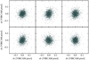 |
Fig. 4 Similar to Fig. 2, but after the boresight correction was applied. The dispersion of the residuals is about 0.035 pixels (~12 mas) along each coordinate. |
3 Proper motions
Proper motions were obtained via a maximum likelihood approach using the affine-invariant Markov chain Monte Carlo method emcee (Foreman-Mackey et al. 2013), to sample the parameter space. This approach allowed us to obtain the posterior probability distribution functions for the quantities μx, μy, x0, y0, where μx, μy are the displacements in the x and y directions, and x0, y0 are the positions at the reference epoch, t0, which we set to be t0 = 2013.0. We ran the Markov Chain Monte Carlo with 32 walkers, performing 5000 steps, with 200 burn-in steps, allowing some scaling on the positional errors as an additional free parameter to be fitted. The medians of the probability distribution functions give our final estimate of μx, μy, x0, y0, and the errors on these quantities were computed as the average between the 16th and 84th percentiles of the samples in the marginalized distributions. The displacements in pixel yr−1 were converted in μα*, μδ by multiplying by the pixel scale that we adopted (0.339 arcsec pixel−1 ), as the master frame axes were already oriented as north and east. At odds with the VIRAC proper motions, which are relative, our proper motions are naturally defined on an absolute system, since their computation is based on the Gaia reference frame.
Figure 5 presents the mean proper-motion errors, σ¯μ =  , as a function of the KS magnitude. Given the extreme crowding environment of the Galactic center, propermotion errors of tile b333 are larger than those of tile b248: the median proper-motion error of sources in the range 12 < KS < 13 – that is, the best measured sources – is 0.58 mas yr−1 in tile b248, compared to 0.70 mas yr−1 in tile b333. Sources with KS ≲ 12 are close to saturation or the nonlinearity regime, and thus their proper-motion errors tend to increase.
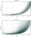 |
Fig. 5 Mean proper-motion errors for sources in tile b248 (top) and tile b333 (bottom) as a function of the KS magnitude. The horizontal line represents the median error of the sources in the range 12 < KS < 13 (see the text for details). |
4 An extension of Gaia into the Galactic plane
Our astrometry is, by construction, linked to the Gaia absolute reference frame. We can see the consistency between Gaia’s and our proper motions in Fig. 6, where we show the residuals between the two datasets, Δμα*, Δμδ, for tile b248 (left) and tile b333 (right). The normalized histograms of the residuals are shown in the right panel of the plots. Dark gray points are the sources with proper-motion errors smaller than 2 mas yr−1 , KS magnitude between 12.5 and 14, Gaia G magnitude between 13 and 18, and measured in at least four individual images1. These objects represent well-measured sources in both sets. The horizontal black line represents the median residuals calculated using the dark gray sources. The standard deviations of the residual distributions are reported in the top right corner of each plot. Given the essentially negligible errors of the Gaia proper motions with respect to ours, the dispersion can be attributed to the random errors on our astrometry. In this regard, we notice that the dispersion is slightly larger than the proper-motions errors obtained by our fit, as is shown in Fig. 5 for sources with KS < 14, suggesting a possible underestimation of the proper-motion errors.
In Fig. 7 we show the local deviations between Gaia s and our proper motions. We divided the field into ~1000 × 1000 pixel regions and, for each region, we calculated the 3σ-clipped medians ( ,
,  ) of the proper-motions residuals. We then computed the quantity
  using only well-measured sources; that is, dark gray points of Fig. 6. From the left panel of Fig. 7, we can notice that the proper motions of tile b248 are in very good agreement with Gaia, and, as was expected, the
  distribution across the tile is flat, with negligible local systematic deviations. The right panel for tile b333 instead shows hints of some spatially dependent systematic errors. We verified that these systematics correlate with the density of Gaia sources in each region, with larger deviations corresponding to regions with very low density. This correlation was expected, as our technique relies on a local net of Gaia sources to compute the boresight correction. Except for these regions with fewer Gaia sources, our proper motions for tile b333 are in good agreement with those in Gaia, with slightly larger residuals with respect to those exhibited by the tile b248, given smaller Gaia source density in tile b333.
Our independent reduction of the VVV fields allows us to extend the Gaia astrometry to the dense and obscured regions of the Galactic plane, providing significantly more new sources with positions and proper motions than what is available from the Gaia DR3 catalog in the same region. Figure 8 shows a J versus (J – KS) color-magnitude diagram of the sources in tile b333. Blue points represent stars in common with the Gaia DR3 catalog. All other objects are in red. It is clear that a large number of sources are not present in the Gaia catalog. Our catalog of tile b333 contains more than 2 million sources with proper motions and only ~10% of them are present in Gaia DR3. In Fig. 9 we show, for the same tile, the source density of the Gaia DR3 catalog (top) and of our catalog (bottom). We used all the sources in our catalog and all the sources in the Gaia catalog for this plot. We computed the values by binning the data into ~3 sq. arcmin bins and smoothing the data out with a Gaussian kernel. In the Galactic center we detect on average ~20 times more sources than Gaia, with regions where this values goes up to ~60.
 |
Fig. 6 Comparison between proper motions computed in this work and Gaia proper motions for tile b248 (left) and tile b333 (right). The black line is the median offset, calculated using the sources in dark gray. |
 |
Fig. 7 Similar to Fig. 6, but as a function of position for tile b248 (left) and tile b333 (right). Each region is colored according to the 3σ-clipped median value of the absolute deviation between Gaia’s and our proper motions, according to the color bars on the right of each panel. |
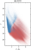 |
Fig. 8 J versus (J – KS) color-magnitude diagram of the sources in tile b333; blue sources are those also present in the Gaia catalog. |
5 Comparison with VIRAC
As a further cross-check, we compared our astrometry with the current public release of the VIRAC catalog (Smith et al. 2018). We crossmatched the Gaia and VIRAC catalogs together, and performed the same comparisons that we described in the previous section. First, in Fig. 10, we show the color-magnitude diagrams of the two tiles built using all the sources in the VIRAC catalog. A comparison between their color-magnitude diagrams and the ones in Fig. 3 shows that our photometry is less affected by saturation effects. Saturation affects sources with KS ≲ 12, and its effect in the photometry is more evident in the color-magnitude diagrams of tile b248, where the VIRAC photometry of the bulge red giant branch exhibits a discontinuity. The color-magnitude diagrams of tile b333 also shows that our catalog is deeper than VIRAC.
Figure 11 is similar to Fig. 6, but for VIRAC sources. Dark gray points represent the sources with a proper-motion error smaller than 2 mas yr−1 and with 12.5 < KS < 14, and with the flag reliable = 1 in the VIRAC catalog, which excludes bad detections and poorly measured stars. We notice that, apart from a global offset with respect to Gaia, the dispersions of the residuals are just slightly larger than ours. Since the formal proper motion errors given by the VIRAC catalog are marginally smaller than ours, we suspect that VIRAC proper-motion errors might also be underestimated.
Finally, in Fig. 12, we show the distribution of the residuals across the field of view, for both tile b248 (left) and b333 (right). Both tiles present significantly larger scatter compared to our work (cf. Fig. 7), with systematic trends that depend on position. It should be noted that VIRAC, unlike our work, does not depend on Gaia, and as such their systematic errors cannot be attributed to the density of Gaia sources. As is pointed out in Smith et al. (2018), VIRAC proper motions are relative to the average motion of sources within a few arcminutes, and in regions with large spatial variations in the extinction, the bulk motion of the reference stars can be different.
In summary, this work represents a step forward with respect to VIRAC, and the most notable improvements are: (i) a larger number of sources with proper motions, mainly thanks to second-pass photometry; (ii) significantly better astrometric precision (about 20–30%) thanks to improved ePSFs, GD, and image-motion correction; and (iii) improved accuracy, thanks to the registration to the absolute reference system of Gaia DR3, which was simply not available at the time of the VIRAC release.
As a final remark, our work uses tools independent of those of VIRAC, and can be leveraged for potential validations or benchmarks for the upcoming VIRAC version 2 (Smith et al., in prep.).
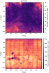 |
Fig. 9 Source density of the Gaia DR3 catalog (top) and of our catalog (bottom) for tile b333 in Galactic coordinates (see the text for details). |
6 Parallax fit
The relatively high cadence of observations within the VVV dataset also enables the measurement of parallaxes, at least for sources close enough to the Sun, so that the effect of the parallax on their apparent motion can be effectively disentangled from that of random positional errors. We tested our parallax fitting procedure on a sample of sources in common with Gaia; in particular, we selected well-measured sources with positions determined in at least 20 epochs, a time baseline of at least three years, a proper motion error smaller than 2 mas yr−1, and with Gaia parallax larger than 5 mas (distance <200 pc). The parallax fit was performed using the Python NOVAS libraries (Barron et al. 2011), adopting the same procedure as in Bedin et al. (2017). Briefly, we calculated the NOVAS predicted source positions at each epoch for a given (α2000, δ2000), proper motion and parallax, where (α2000, δ2000) are the positions at epoch 2000.0. We then computed the differences between these positions and those measured by us, and we looked for the astrometric solution that minimizes these differences, using the same MCMC approach that we employed for the proper motion fit.
In Fig. 13, we show an example of the parallax fit for four selected sources (two per tile). We report in the plot the fitted proper motion and parallax values, together with the values given in the Gaia DR3 catalog. Sources in Figs. 13a and b are in agreement within 2σ, while those in Figs. 13c and d are compatible within 1σ with the Gaia parallaxes.
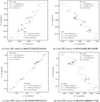 |
Fig. 13 Example of parallax fit for four sources in common with Gaia: panels a and b are for sources in tile b248, while sources in panels c and d are in tile b333. Coordinates are relative to (α0, δ0) chosen as the mean position between the first and last epochs. |
7 Data reduction strategy and access
We plan to process the entire VVV dataset, starting from the innermost bulge fields. However, we will also accept requests from the astronomical community to prioritize particular VVV or VVVx tiles. The catalogs of the first two tiles presented in this work have been made available online2. This repository will be constantly updated with new products once they are ready. For reasonable requests, we can also provide artificial star tests and astro-photometric time series.
8 Conclusion
In this paper, we exploited the VVV data to extend the Gaia astrometry into the Galactic plane, focusing on two pilot fields, one in the Galactic center and the other in the southeast bulge. We were able to significantly improve astrometric precision and completeness with respect to previous efforts. These improvements are achieved through a combination of state-of-the-art techniques: (i) the use of spatially variable ePSFs for precise position and flux measurements; (ii) local transformations, which allow us to mitigate systematic errors, most notably residual GD and atmospheric effects; and (iii) a combination of first-and second-pass photometry to improve the detection of faint stars in crowded fields, which allows us to detect significantly more sources than previous efforts in the literature. Our astrom-etry is anchored to the Gaia DR3 reference frame, and represents an extension of Gaia accuracy into the Galactic plane. In future releases, we plan to also include the VVVx data to increase the number of pawprints and extend the temporal baseline available for each tile. We will also combine the information from adjacent tiles in order to measure accurate proper motions for sources near the borders of the tiles, too.
Acknowledgements
M.G. and A.B. acknowledge support by STScI DRF D0001.82523. M.G. and L.R.B. acknowledge support by MIUR under PRIN program #2017Z2HSMF and by PRIN-INAF 2019 under program #10-Bedin. D.M. gratefully acknowledges support from the ANID BASAL projects ACE210002 and FB210003, from Fondecyt Project No. 1220724, and from CNPq Brasil Project 350104/2022-0. The authors thank Maren Hempel for providing the VVV tiles pointing data.
References
- Anderson, J., & van der Marel, R. P. 2010, ApJ, 710, 1032 [NASA ADS] [CrossRef] [Google Scholar]
- Anderson, J., Bedin, L. R., Piotto, G., Yadav, R. S., & Bellini, A. 2006, A&A, 454, 1029 [NASA ADS] [CrossRef] [EDP Sciences] [Google Scholar]
- Anderson, J., King, I. R., Richer, H. B., et al. 2008a, AJ, 135, 2114 [NASA ADS] [CrossRef] [Google Scholar]
- Anderson, J., Sarajedini, A., Bedin, L. R., et al. 2008b, AJ, 135, 2055 [Google Scholar]
- Barbuy, B., Chiappini, C., & Gerhard, O. 2018, ARA&A, 56, 223 [Google Scholar]
- Barron, E. G., Kaplan, G. H., Bangert, J., et al. 2011, AAS Meeting Abs., 217, 344.14 [NASA ADS] [Google Scholar]
- Bedin, L. R., & Fontanive, C. 2018, MNRAS, 481, 5339 [NASA ADS] [CrossRef] [Google Scholar]
- Bedin, L. R., & Fontanive, C. 2020, MNRAS, 494, 2068 [NASA ADS] [CrossRef] [Google Scholar]
- Bedin, L. R., Salaris, M., Piotto, G., et al. 2009, ApJ, 697, 965 [NASA ADS] [CrossRef] [Google Scholar]
- Bedin, L. R., Ruiz-Lapuente, P., Gonzalez Hernandez, J. I., et al. 2014, MNRAS, 439, 354 [NASA ADS] [CrossRef] [Google Scholar]
- Bedin, L. R., Pourbaix, D., Apai, D., et al. 2017, MNRAS, 470, 1140 [NASA ADS] [CrossRef] [Google Scholar]
- Bellini, A., Anderson, J., Bedin, L. R., et al. 2017, ApJ, 842, 6 [NASA ADS] [CrossRef] [Google Scholar]
- Contreras Ramos, R., Minniti, D., Fernandez-Trincado, J. G., et al. 2018, ApJ, 863, 78 [NASA ADS] [CrossRef] [Google Scholar]
- Fabricius, C., Luri, X., Arenou, F., et al. 2021, A&A, 649, A5 [NASA ADS] [CrossRef] [EDP Sciences] [Google Scholar]
- Foreman-Mackey, D., Hogg, D. W., Lang, D., & Goodman, J. 2013, PASP, 125, 306 [Google Scholar]
- Fragkoudi, F., Di Matteo, P., Haywood, M., et al. 2020, in IAU General Assembly, 282 [Google Scholar]
- Gaia Collaboration (Prusti, T., et al.) 2016, A&A, 595, A1 [NASA ADS] [CrossRef] [EDP Sciences] [Google Scholar]
- Gaia Collaboration (Vallenari, A., et al.) 2023, A&A, 674, A1 [NASA ADS] [CrossRef] [EDP Sciences] [Google Scholar]
- Garro, E. R., Minniti, D., Gómez, M., et al. 2020, A&A, 642, L19 [EDP Sciences] [Google Scholar]
- Garro, E. R., Minniti, D., Alessi, B., et al. 2022a, A&A, 659, A155 [NASA ADS] [CrossRef] [EDP Sciences] [Google Scholar]
- Garro, E. R., Minniti, D., Gómez, M., et al. 2022b, A&A, 662, A95 [NASA ADS] [CrossRef] [EDP Sciences] [Google Scholar]
- Gonzalez-Fernandez, C., Hodgkin, S. T., Irwin, M. J., et al. 2018, MNRAS, 474, 5459 [CrossRef] [Google Scholar]
- Griggio, M., Bedin, L. R., Raddi, R., et al. 2022, MNRAS, 515, 1841 [NASA ADS] [Google Scholar]
- Griggio, M., Salaris, M., Nardiello, D., et al. 2023, MNRAS, 524, 108 [Google Scholar]
- Häberle, M., Libralato, M., Bellini, A., et al. 2021, MNRAS, 503, 1490 [CrossRef] [Google Scholar]
- Hajdu, G., Dékány, I., Catelan, M., & Grebel, E. K. 2020, Exp. Astron., 49, 217 [Google Scholar]
- Irwin, M. J., Lewis, J., Hodgkin, S., et al. 2004, SPIE Conf. Ser., 5493, 411 [Google Scholar]
- Kader, J. A., Pilachowski, C. A., Johnson, C. I., et al. 2022, ApJ, 940, 76 [NASA ADS] [CrossRef] [Google Scholar]
- Lewis, J. R., Irwin, M., & Bunclark, P. 2010, ASP Conf. Ser., 434, 91 [Google Scholar]
- Libralato, M., Bellini, A., Bedin, L. R., et al. 2014, A&A, 563, A80 [NASA ADS] [CrossRef] [EDP Sciences] [Google Scholar]
- Libralato, M., Bellini, A., Bedin, L. R., et al. 2015, MNRAS, 450, 1664 [NASA ADS] [CrossRef] [Google Scholar]
- Libralato, M., Lennon, D. J., Bellini, A., et al. 2021, MNRAS, 500, 3213 [Google Scholar]
- Minniti, D. 2018, The Vatican Observatory, Castel Gandolfo: 80th Anniversary Celebration, in Astrophysics and Space Science Proceedings, eds. G. Gionti, & J.-B. Kikwaya Eluo (Berlin: Springer), 51, 63 [NASA ADS] [CrossRef] [Google Scholar]
- Minniti, D., Lucas, P. W., Emerson, J. P., et al. 2010, New Astron., 15, 433 [Google Scholar]
- Minniti, D., Geisler, D., Alonso-García, J., et al. 2017, ApJ, 849, L24 [CrossRef] [Google Scholar]
- Minniti, D., Fernández-Trincado, J. G., Gómez, M., et al. 2021a, A&A, 650, L11 [NASA ADS] [CrossRef] [EDP Sciences] [Google Scholar]
- Minniti, D., Fernández-Trincado, J. G., Smith, L. C., et al. 2021b, A&A, 648, A86 [NASA ADS] [CrossRef] [EDP Sciences] [Google Scholar]
- Minniti, D., Matsunaga, N., Fernandez-Trincado, J. G., et al. 2024, A&A, 683, A150 [NASA ADS] [CrossRef] [EDP Sciences] [Google Scholar]
- Mróz, P., Udalski, A., Skowron, J., et al. 2019, ApJS, 244, 29 [Google Scholar]
- Platais, I., Kozhurina-Platais, V., Girard, T. M., et al. 2002, AJ, 124, 601 [NASA ADS] [CrossRef] [Google Scholar]
- Platais, I., Wyse, R. F. G., & Zacharias, N. 2006, PASP, 118, 107 [NASA ADS] [CrossRef] [Google Scholar]
- Scalco, M., Bellini, A., Bedin, L. R., et al. 2021, MNRAS, 505, 3549 [NASA ADS] [CrossRef] [Google Scholar]
- Skrutskie, M. F., Cutri, R. M., Stiening, R., et al. 2006, AJ, 131, 1163 [NASA ADS] [CrossRef] [Google Scholar]
- Smith, L. C., Lucas, P. W., Kurtev, R., et al. 2018, MNRAS, 474, 1826 [Google Scholar]
- Zoccali, M. 2019, Boletin de la Asociacion Argentina de Astronomia La Plata Argentina, 61, 137 [NASA ADS] [Google Scholar]
All Figures
|
Fig. 1 Gaia DR3 source density around the region covered by the VVV survey. White boxes represent VVV tiles. We highlight in light blue the two tiles considered in this work; namely, b333 in the Galactic center and b248 on the southern bulge. Density map data were taken from the Gaia archive. |
| In the text | |
|
Fig. 2 Positional residuals obtained by crossmatching the catalogs of a set of consecutive images with Gaia after the GD solution derived with the VVV dataset was applied. Each panel corresponds to a distinct image. The residuals display different trends, preventing a precision of less than ~0.1 pixels (~35 mas) in a single exposure with this approach. |
| In the text | |
|
Fig. 3 Color-magnitude diagrams for tiles b248 (left) and b333 (right); see the text for details. |
| In the text | |
|
Fig. 4 Similar to Fig. 2, but after the boresight correction was applied. The dispersion of the residuals is about 0.035 pixels (~12 mas) along each coordinate. |
| In the text | |
|
Fig. 5 Mean proper-motion errors for sources in tile b248 (top) and tile b333 (bottom) as a function of the KS magnitude. The horizontal line represents the median error of the sources in the range 12 < KS < 13 (see the text for details). |
| In the text | |
|
Fig. 6 Comparison between proper motions computed in this work and Gaia proper motions for tile b248 (left) and tile b333 (right). The black line is the median offset, calculated using the sources in dark gray. |
| In the text | |
|
Fig. 7 Similar to Fig. 6, but as a function of position for tile b248 (left) and tile b333 (right). Each region is colored according to the 3σ-clipped median value of the absolute deviation between Gaia’s and our proper motions, according to the color bars on the right of each panel. |
| In the text | |
|
Fig. 8 J versus (J – KS) color-magnitude diagram of the sources in tile b333; blue sources are those also present in the Gaia catalog. |
| In the text | |
|
Fig. 9 Source density of the Gaia DR3 catalog (top) and of our catalog (bottom) for tile b333 in Galactic coordinates (see the text for details). |
| In the text | |
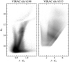 |
Fig. 10 Similar to Fig. 3, but for VIRAC sources. |
| In the text | |
 |
Fig. 11 Similar to Fig. 6, but for VIRAC sources. |
| In the text | |
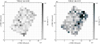 |
Fig. 12 Similar to Fig. 7, but for VIRAC sources. |
| In the text | |
|
Fig. 13 Example of parallax fit for four sources in common with Gaia: panels a and b are for sources in tile b248, while sources in panels c and d are in tile b333. Coordinates are relative to (α0, δ0) chosen as the mean position between the first and last epochs. |
| In the text | |
Current usage metrics show cumulative count of Article Views (full-text article views including HTML views, PDF and ePub downloads, according to the available data) and Abstracts Views on Vision4Press platform.
Data correspond to usage on the plateform after 2015. The current usage metrics is available 48-96 hours after online publication and is updated daily on week days.
Initial download of the metrics may take a while.