| Issue |
A&A
Volume 687, July 2024
|
|
|---|---|---|
| Article Number | A215 | |
| Number of page(s) | 18 | |
| Section | Stellar structure and evolution | |
| DOI | https://doi.org/10.1051/0004-6361/202349065 | |
| Published online | 15 July 2024 | |
Evolutionary nature of puffed-up stripped star binaries and their occurrence in stellar populations
1
Department of Physics, Indian Institute of Technology Palakkad, Kerala, India
e-mail: debasishdutta1707@gmail.com
2
European Southern Observatory, Karl-Schwarzschild-Strasse 2, 85748 Garching bei München, Germany
e-mail: Jakub.Klencki@eso.org
Received:
22
December
2023
Accepted:
8
April
2024
The majority of massive stars are formed in multiple systems, and at some point during their life, they interact with their companions via mass transfer. This interaction typically leads to the primary shedding its outer envelope, resulting in the formation of a “stripped star”. Classically, stripped stars are expected to quickly contract to become hot and UV-bright helium stars. Surprisingly, recent optical spectroscopic surveys have unveiled many stripped stars that are much larger and cooler, appearing “puffed up” and overlapping with the Main Sequence (MS) in the Hertzsprung–Russell diagram. Here, we study the evolutionary nature of puffed-up stripped (PS) stars and the duration of this enigmatic phase using the stellar-evolution code MESA. We computed grids of binary models at four metallicities: Solar (Z⊙ = 0.017), Large Magellanic Cloud (LMC, Z = 0.0068), Small Magellanic Cloud (SMC, Z = 0.0034), and Z = 0.1 Z⊙. Contrary to previous assumptions, we find that stripped stars regain thermal equilibrium shortly after the end of mass transfer and maintain it during most of the PS phase. Their further contraction towards hot and compact He stars is determined by the rate at which the residual H-rich envelope is depleted, with the main agents being H-shell burning (dominant for M ≲ 50 M⊙) and mass-loss in winds. The duration of the PS star phase is approximately 10% of the core-He burning lifetime (1% total lifetime) and up to 100 times more than the thermal timescale. It decreases with increasing mass and luminosity and increases with metallicity. We explored several factors influencing PS star lifetimes: orbital period, mass ratio, winds, and semiconvection. We further carried out a simple binary population synthesis estimation, finding that ∼0.5–0.7% of all the stars with log (L/L⊙) > 3.7 may, in fact, be PS stars. Our results indicate that tens to hundreds of PS stars in post-interaction binaries may be hiding in the MS population, disguised as ‘normal’ stars: ∼100 (∼280) in the SMC (LMC) and ∼1500 in the Milky Way. Their true nature may be revealed by spectroscopically measured low surface gravities, high N enrichment, and likely slow rotation rates.
Key words: binaries: close / binaries: general / stars: evolution / stars: massive
© The Authors 2024
 Open Access article, published by EDP Sciences, under the terms of the Creative Commons Attribution License (https://creativecommons.org/licenses/by/4.0), which permits unrestricted use, distribution, and reproduction in any medium, provided the original work is properly cited.
This article is published in open access under the Subscribe to Open model. Subscribe to A&A to support open access publication.
1. Introduction
Binary stars form a significant portion of the stellar population. Approximately 40% of low-mass stars (0.8–1.2 M⊙) exist within binary or multiple systems (Moe & Di Stefano 2017). This prevalence is even more pronounced among massive stars (M ≳ 8 M⊙), where binary systems overwhelmingly dominate the overall population (Sana et al. 2012, 2014). Around 94% of massive stars with masses ≳16 M⊙ exist within binary or multiple systems (Moe & Di Stefano 2017), where most of them engage in interactions with companion stars, involving the transfer of mass and angular momentum. During mass transfer, the more massive star, often referred to as the primary star, transfers material to its less massive companion through a process known as Roche Lobe Overflow (RLOF). This can lead to the primary star shedding its outer envelope, resulting in the formation of what is known as a ‘stripped star’. A large fraction of massive binaries (∼30%) go through envelope stripping (Sana et al. 2012) and therefore are more common (Podsiadlowski et al. 1992; Eldridge et al. 2013; Götberg et al. 2019; Shao & Li 2021). Due to their very high temperatures, stripped stars serve as an important source for ionising photons. They are considered to have contributed to cosmic reionisation (Götberg et al. 2018, 2020a). They are recognised as progenitors of stripped-envelope supernovae (Smith et al. 2011; Yoon et al. 2017) and are also deemed to be one of the key contributors to the population of gravitational wave progenitors, leading to the formation of merging pairs of neutron stars (NSs) and black holes (BHs) (Kalogera et al. 2007; Götberg et al. 2020b).
Stripped stars are most commonly formed when the primary star donates mass to its companion during stable mass transfer initiated due to rapid expansion after the end of the main sequence (crossing the Hertzsprung gap). During this process, the donor star rapidly loses its entire hydrogen envelope during a short-lived phase of thermal timescale mass exchange (≲104 years) (Kippenhahn & Weigert 1967; van den Heuvel 1975; Podsiadlowski et al. 1992; Vanbeveren et al. 1998) (see however, Klencki et al. 2022, where it is shown that the mass transfer can also occur at nuclear timescale in case of low metallicity massive donors). This kind of mass transfer is referred to as case B mass transfer (Kippenhahn & Weigert 1967; Paczyński 1967; Wellstein et al. 2001) and is the most common channel for mass transfer of stars in binaries (de Mink et al. 2008; Götberg et al. 2017; Vartanyan et al. 2021). Stripped stars can also be formed when stable mass transfer occurs during the main sequence (referred to as case A; Wellstein et al. 2001), or after the ejection of a common envelope formed as a result of unstable mass transfer (Kippenhahn & Weigert 1967; Ivanova 2011). Stars undergoing mass loss through these processes often result in the formation of stripped stars of various kinds, contributing to a diverse range from subdwarfs to Wolf Rayet (WR) stars (Paczyński 1967; van den Heuvel 1975; Vanbeveren 1991; Podsiadlowski et al. 1992; De Loore & De Greve 1992; Petrovic et al. 2005; Eldridge et al. 2008; Götberg et al. 2017; Laplace et al. 2020). Subdwarfs are stars with masses up to about 1.5 M⊙, which correspond to initial masses of up to about 7 M⊙ and account for low mass stripped stars. WR stars have masses ≳8 M⊙ (although this depends strongly on metallicity, see for example Shenar et al. 2020b) and accounts for the massive stripped stars. Intermediate mass-stripped stars primarily refer to stars with mass between ∼1 and 8 M⊙ (progenitor masses between 8 and 25 M⊙).
After the mass transfer, these stars subsequently transition into hot, compact helium stars (e.g., Kippenhahn 1969; Götberg et al. 2017, 2018; Laplace et al. 2020, 2021; Klencki et al. 2022). This phase spans about 10% of the star’s entire lifespan (Götberg et al. 2017, 2018), with its primary source of energy arising from helium fusion through the triple-alpha reaction occurring in the core. However, most emitted light during this stage primarily occurs in the ultraviolet (UV) range, rendering it inaccessible to observation by ground-based telescopes (Götberg et al. 2017). This region is characterised by very high temperatures and populated by subdwarf O (sdO) stars and WR stars (see Götberg et al. 2017, 2018). A handful of such systems are observed till date, including sdO stars like ϕ Persei (Gies et al. 1998), 59 Cyg (Peters et al. 2013), and 60 Cyg (Wang et al. 2017), along with a quasi-WR star identified in HD 45166 (Steiner & Oliveira 2005; Groh et al. 2008; Shenar et al. 2023). Additionally, a sample of Galactic sdOs have been reported by Wang et al. (2018, 2021). Notably, Drout et al. (2023) have recently reported a sample of 25 stars in the Magellanic Clouds. These stars exhibit characteristics in line with the expected properties of intermediate mass-stripped stars, encompassing mass ranges from 1 to 9 M⊙, as discussed in Götberg et al. (2023).
Interestingly, recent observations have detected systems that have recently detached from mass transfer and have not yet settled as a hot and compact helium star. These stars are characterised by larger radii and cooler effective temperatures than classical ‘hot’ stripped stars and are prevalent as ‘bloated stripped stars’ in recent literature (Bodensteiner et al. 2020; El-Badry & Burdge 2022; Villaseñor et al. 2023, etc.). They are visible in the optical spectrum due to their relatively cooler surface temperatures than the hot-stripped stars. However, they pose a challenge in terms of accurate identification, as they resemble normal B-type stars with their HR diagram position (temperatures and luminosities) often overlapping with the MS. Their true nature is revealed in spectroscopy when the surface abundances (in particular enhanced N) and relatively small gravities (leading to low spectroscopic masses) are measured. However, this measurement is not an easy task since they are usually accompanied by a rapidly rotating companion with a similar spectral type, making it difficult to disentangle the cool stripped star from the combined spectra of the binary without sufficient spectral resolution and multi-epoch data.
One famous example is LB-1, which was reported by Liu et al. (2019) as a ∼70 M⊙ BH. However, Shenar et al. (2020a) subsequently presented an alternative interpretation, suggesting that the system could be better explained as comprising a ‘puffed-up’ stripped star with a mass of 1.5 M⊙, accompanied by a Be companion weighing 7 M⊙. Another example is HR 6819, which was proposed as a triple system containing a BH in the inner binary by Rivinius et al. (2020). However, Bodensteiner et al. (2020) (also El-Badry & Quataert 2021) found it to contain a ‘puffed-up’ stripped star of mass 0.56 M⊙. Similar ambiguity surrounds NGC 1850 BH1, initially proposed as an 11 M⊙ BH by Saracino et al. (2022) but later suggested to be a ‘puffed-up’ stripped star with a mass between 0.65 and 1.5 M⊙ (El-Badry & Burdge 2022).
The examples above involve low-mass stripped stars (Mstripped ≲ 1.5). Among intermediate mass stripped stars (Mstripped∼ 1−8 M⊙) is the γ Columbae, which was reported by Irrgang et al. (2022) as a partially stripped pulsating core (∼4 − 5 M⊙) of a massive star of roughly 12 M⊙ at solar metallicity. However, no companion was detected. Recently, Ramachandran et al. (2023) discovered the first stripped star of intermediate-mass in low metallicity, SMCSGS-FS 69. This star was found to be a puffed-up stripped star (∼3 M⊙) originating from a massive star of ∼12 M⊙ and is currently transitioning towards the hotter part in the HR diagram. Among the other recently discovered ones are VFTS 291 (∼1.5 − 2.5 M⊙) (Villaseñor et al. 2023) and the so-called star 16 (∼0.8 M⊙) from the recently reported sample of 25 stars by Drout et al. (2023) and Götberg et al. (2023).
The phase of evolution where these puffed-up stripped stars are found ranges from post-RLOF to the moment where the companion outshines the primary in the optical spectra. Classically, this immediate post-RLOF contraction phase is perceived as a short-lived temporary stage, with the duration likely characterised by the thermal timescale of the stripped donor (≲104 yr). This, however, would correspond to only < 0.1% of the total stellar lifetime, most likely at odds with the number of puffed-up stripped stars detected so far. This conundrum was noted by El-Badry & Quataert (2021), who briefly pointed out that the duration of the post-RLOF contraction and the puffed-up stripped star phase in their models are much longer than the thermal timescale. However, a comprehensive theoretical investigation focused on this specific phase of binary star evolution is still missing.
Consequently, this paper endeavours to fill this gap by offering an in-depth examination of the immediate post-RLOF phase. Our focus centres on unravelling the intricate evolution of these puffed-up stripped stars. For this purpose, we generate grids of binary models between 5 and 40 M⊙ at four distinct metallicities: solar metallicity (Z = 0.017), Large Magellanic Cloud (LMC) metallicity (Z = 0.0068), Small Magellanic Cloud (SMC) metallicity (Z = 0.0034) and Z = 0.1 Z⊙ = 0.0017. We also investigate several factors that could potentially impact the duration of the contraction phase, such as orbital period, mass ratio, wind mass loss rate and semiconvection. Furthermore, we also estimate the number of puffed-up stripped stars one can expect to find in the Small and Large Magellanic Clouds (S/LMCs).
The structure of the paper is as follows: In Sect. 2, we outline our computational method and the physical assumptions underlying our study; in Sect. 3, we perform a detailed investigation of one particular binary model, and further discuss the full grids of evolutionary models. In Sect. 4, we discuss the uncertainties and estimate the number of puffed-up stripped stars (PSS) that we predict to exist in young stellar populations and compare our default definition of the puffed-up stripped star phase with another criterion. We summarise and conclude our findings in Sect. 5.
2. Method: Binary stellar evolution models
2.1. Physical ingredients
We construct binary evolution models using the 1D stellar evolution code MESA (Paxton et al. 2011, 2013, 2015, 2018, 2019) (version 11540). Models were computed using four distinct initial chemical compositions. For solar metallicity, we assumed Z⊙ = 0.017 and abundance ratios as outlined by Grevesse & Sauval (1998) (also Grevesse et al. 1996). In the case of sub-solar metallicities, we computed our models using abundance ratios of the Magellanic Clouds following Brott et al. (2011), where we used Z = 0.0068 (0.4 Z⊙) for Large Magellanic Clouds (LMC), Z = 0.0034 (0.2 Z⊙) for the Small Magellanic Clouds (SMC). We also computed our models using Z = 0.0017 (0.1 Z⊙). In our models, all stars are assumed to be non-rotating. We employ the standard basic.net nuclear network, comprising eight distinct species. Additionally, we make use of the default MESA opacity tables in our analysis (Iglesias & Rogers 1993, 1996; Buchler & Yueh 1976; Cassisi et al. 2007).
Convection is modelled as per the mixing length theory (Böhm-Vitense 1958) with a mixing length of 2.0 times the pressure scale height. We adopted the Ledoux criterion for convection and accounted for semiconvective mixing with an efficiency parameter of αSC = 0.01. While αSC has a limited effect on main sequence (MS) donors, its effect on post-MS is enormous (Klencki et al. 2020). We studied the effect of high semiconvection in Appendix B. We accounted for convective core-overshooting by applying exponential overshooting (Herwig 2000), with a parameter f = 0.0425. It is important to note that convective motion comes to a halt at the boundary of a convective zone. However, to account for exponential overshooting beyond this boundary, we consider an additional parameter, f0 = 0.001. We also considered the thermohaline mixing (Kippenhahn et al. 1980) with thermohaline coefficient = 2.0. However, earlier studies have shown that thermohaline mixing has little impact on the stellar structures of stripped stars (Yoon et al. 2017; Götberg et al. 2017). To help converge models approaching the Eddington limit, we applied a reduction of superadiabacity in radiation-dominated regions (Sect. 7.2 of Jermyn et al. 2023).
To compute the interaction involving a binary system, we employ the implicit mass-transfer approach proposed by Kolb & Ritter (1990) for the RLOF. The main goal of this paper is to analyse the behaviour of the donor star following the RLOF, aiming to comprehend the extended duration of the subsequent contraction phase. Therefore, for simplicity, we exclusively track the evolutionary path of the primary (donor) star, treating the companion as a point mass equal to 0.6 of the initial primary mass. We assume the accretion efficiency of 100%. Our focus primarily revolves around stripped-envelope stars generated through mass transfer from stars that fill their Roche lobes due to swift expansion during the hydrogen shell-burning phase after departing from the main sequence. A minority of cases also involve consideration of case A mass transfer. Furthermore, we incorporate the influence of tidal forces using the methodology outlined by Hut (1981). It is important to note that tidal effects are not significant in massive case B binaries.
We modelled stellar winds following the default ‘Dutch’ wind scheme of MESA (Paxton et al. 2011). This approach for massive stars combines findings from various studies, mostly done by people from the Netherlands. The specific amalgamation incorporated within MESA derives from the work of Glebbeek et al. (2009). This scheme uses the mass loss rates of Vink et al. (2001) for Teff ≥ 104 and surface H > 0.4 (hydrogen-rich) and the rates of Nugis & Lamers (2000) for Teff ≥ 104 and surface H < 0.4 (hydrogen-poor). Vink et al. (2001) includes a metallicity dependence of Ṁ ∝ (Z/Z⊙)0.85 and in the case of Nugis & Lamers (2000), it is Ṁ ∝ Z0.47. The Reimers_scaling_factor for cool stars and Dutch_scaling_factor for hot stars are set to 1.
2.2. Initial parameter space and stopping conditions
Models are computed with four different chemical compositions: solar (Z⊙), LMC (0.4 Z⊙), SMC (0.2 Z⊙), and 0.1 Z⊙. Each grid spans 14 initial primary masses M1: 5, 6.5, 8, 10, 12, 16, 16.9, 20, 22, 26, 30, 32, 36 and 40 M⊙. The default initial mass ratio qini = M2/M1 and the default initial orbital period Pini are set to be 0.6 and 70 days, respectively. We have computed additional models encompassing various mass transfer sequences, where q ranges from 0.4 to 1.0, and the initial orbital period Pini spans 10 to 100 days. We have terminated our models at central Helium depletion (Y < 10−6). For demonstration purposes, we have terminated some of our models (Figs. 1 and 5) at core Carbon depletion (XC < 10−6). The puffed-up stripped star phase is considered from the immediate post-RLOF moment until the effective temperature is 0.1 dex higher than that of the Zero Age Main sequence (ZAMS) temperature of the primary. We discuss this choice and compare it to a different criterion further in Sect. 4.1.
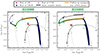 |
Fig. 1. Hertzsprung–Russel diagram of two representative binary models of 16 M⊙ at metallicities 0.0068 (LMC) and 0.0017(0.1 Z⊙) starting from main sequence (MS) till core carbon depletion. Dotted diagonal lines represent lines of constant radius. The evolution stages are marked and labelled in various colours. The red dot represents the end of the main sequence (MS), and the blue square and pink diamond represent the end of core He burning (CHeB) and core carbon burning (CCB), respectively. The blue region represents the mass transfer phase, and the orange region shows the puffed-up stripped star (PSS) phase. Letters A to I mark the important instances in the star’s evolution (see text). The grey track ( |

3. Results
3.1. Exploring evolutionary models
In this section, we delve into our findings by closely examining binary models characterised by an initial primary mass of 16 M⊙ along with initial orbital period Pini = 70 days and mass ratio qini = 0.6. These models are examined under two distinct metallicities: LMC (Z = 0.4 Z⊙ = 0.0068) metallicity and Z = 0.0017. Figure 1 shows the HR diagram of the primary in both cases. The blue lines represent the RLOF phase, and the orange lines represent the puffed-up stripped star phase, defined as the stage between the end of the RLOF and the point when the stripped donor becomes hotter than its ZAMS position plus 0.1 dex in log Teff. As we discuss further, this ad hoc temperature threshold approximates the regime when the stripped star is still comparably bright in the optical bands to its likely companion and can most easily be detected without resorting to UV.
To comprehend the mechanisms governing the evolution of the star, we analyse the important factors. In Fig. 2 (also see Figs. D.2 and D.1), a magnified view of various parameters during the contraction phase is presented. The lowest panel d displays the different luminosities contributing to energy output. Notably, the dashed red line (Lgrav) represents the amount of energy per unit of time related to changes in the gravitational energy of the star. This luminosity is the integral of gravitational energy generation rate per unit mass ϵgrav, where ϵgrav is a local quantity. When Lgrav is positive, it signifies that the star is undergoing self-contraction due to its own gravity. Consequently, when Lgrav is positive, then part of the surface luminosity of the star is due to rapid structural changes (e.g., core contraction). Conversely, Lgrav being negative indicates that its surface luminosity is lower than that produced in nuclear burning as part of the nuclear energy is used to increase the gravitational potential energy of the star.
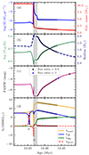 |
Fig. 2. Evolution of various quantities of a 16 M⊙ model (at LMC metallicity) with star age, near the mass transfer phase leading up to the puffed-up stripped star (PSS) phase. Panel (a) shows the variation of envelope mass and mass loss rate of the donor. The mass loss is mainly due to the transfer of mass to the companion but also contains contribution from winds. Panel (b) shows the effective temperature (green) and donor radius (blue), and panel (c) shows the magnitude computed in the F450W optical filter of the HST WFPC2 camera. The blue triangle and the black star represent the position where the flux ratio (fstripped/fcompanion) drops below 1 and 0.5, respectively. Panel (d) represents various luminosities contributing to the total energy output: the orange line represents the surface luminosity (Lsurf), the blue and green lines represent the luminosity to hydrogen burning (LH) and helium burning (LHe) respectively. The luminosity in the red dashed line is the luminosity due to gravitational contraction/expansion (Lgrav). The grey-shaded region represents the mass transfer phase, and the regions with dark lines represent the puffed-up stripped star (PSS) phase. |
In the following sections, we describe the important stages in the evolution of the primary star, starting from the main sequence till the end of core Helium burning. For an exemplary choice, we take the 16 M⊙ model at LMC metallicity (Z = 0.0068) and also compare it with the lower metallicity model (Z = 0.0017).
3.1.1. Evolution until RLOF
The main-sequence evolution of our primary stars (labelled A-B in Fig. 1) closely follows the evolution of a single star. The star burns hydrogen into helium in a convective core, with the low-metallicity model being slightly more compact and hotter during the MS due to smaller opacity. After the end of MS (B), the core contracts while the outer layers expand. In Fig. 2, we see that Lgrav increases to nearly equal to the surface luminosity (|Lgrav|/Lsurf ∼ 0.8), which means that most of the energy is generated from contraction within the star and the shell burning has not kicked in yet. This coincides with a slight increase in Teff, a very brief phase just before point B. As a result of this contraction of the star, the shell gets hot, and LH quickly increases, which in turn causes the outer layers (envelope) to expand, and the star moves to cooler effective temperatures. The H shell burning starts pretty much straight after the end of the MS, and it is this increase in LH that puffs up the star (Farrell et al. 2022).
The star continues to expand on a thermal timescale until it fills its Roche lobe, prompting the transfer of matter to its companion. If the star had not been in a binary configuration, it would have followed the trajectory in grey colour ( ) (Fig. 1). During mass transfer, as the donor loses a significant amount of mass from its outer layers, a significant fraction of its burning luminosity is trapped in the expanding envelope and used to readjust the stellar structure (|Lgrav|/LH ∼ 0.77 when the mass loss (ML) rate peaks, see Fig. 2). During the entire mass transfer phase lasting approximately 0.013 Myr, the donor sheds most of its H-rich envelope (nearly 85% of the envelope mass it had before RLOF), leaving behind only ∼1.6 M⊙ of the envelope. Notably, the energy generation in shell burning (LH) is only weakly affected by the interaction and LH returns to a value even greater than its pre-RLOF value (see Fig. 2)
3.1.2. The “contraction phase”
Once the mass transfer ceases, we are left with a helium-rich star (Mcore ≈ 5.4 M⊙, XHe; center ≈ 0.99) encased in a small hydrogen envelope of ∼1.6 M⊙. The question of how much envelope mass is left unstripped after the RLOF is closely connected to factors such as metallicity, the internal envelope structure, and the wind mass loss rate. At lower metallicities, stars retain a larger part of the H-rich envelope after the mass transfer (Götberg et al. 2017; Yoon et al. 2017; Laplace et al. 2020; Klencki et al. 2022). For example, in our 16 M⊙ model with solar metallicity, the mass of the H envelope left after the mass transfer is ∼1.3 M⊙, whereas in the case of LMC it is ∼1.6 M⊙. This preservation of a larger envelope in lower metallicity models arises from the diminishing efficiency of the stripping procedure under conditions of lower metallicity as a consequence of the decreased opacity observed in the outer layers. When opacity is decreased, a larger portion of the hydrogen-rich envelope stays within the Roche lobe, subsequent to the detachment of the stars. When the rates of wind mass loss are lower, either due to intrinsic factors or due to lower metallicity (e.g., Sander & Vink 2020), stars lose less mass in the subsequent post-mass transfer evolution, such that there are more likely to retain H even until the end of their evolution and a supernova.
Eventually, after a phase of post-RLOF contraction, the star evolves into a hot, compact helium star, deriving its primary energy from helium fusion through the triple-alpha reaction at its core. This stage is the longest-lived phase in the lifecycle of a stripped star, spanning almost 10% of its total lifetime. It is marked by point G in Fig. 1. However, before the star settles down as a helium star, it undergoes a transition phase (E-F). The stars in this phase are somewhat cooler and more puffed-up than the hot and compact He stars. Due to this, they are visible in the optical spectrum. We denote this stage as the puffed-up stripped star (PSS) phase throughout this paper and discuss it in more detail in the following section.
3.2. A closer look at the contraction phase
The dynamics of contraction or expansion of a star can be explained through the examination of its gravitational luminosity (Lgrav) (as mentioned in Sect. 3.1). The contribution of Lgrav is generally insignificant during phases of hydrostatic and thermal equilibrium (|Lgrav|/Lsurf ∼ 0.01 during MS). However, there is a distinct surge in its magnitude towards the end of the main sequence (MS) phase (the point marked B in Fig. 1 and see Fig. 2), where |Lgrav|/Lsurf ∼ 0.9 and |Lgrav|/LH ∼ 8. This phenomenon arises from the depletion of hydrogen in the core (indicated by a dip in the hydrogen-burning luminosity), prompting core contraction to restore equilibrium. As the core contracts, the envelope expands, causing a subsequent reduction and eventual inversion of Lgrav’its value turns negative. The point of highest magnitude in Lgrav is achieved as the star enters the phase of mass transfer, characterised by a substantial negative peak (|Lgrav| / Lsurf ∼ 3.24 and |Lgrav| / LH ∼ 0.77). This phase is very brief and aligns with the period of maximum mass transfer rate (top panel (blue) of Fig. 2). Following this peak, the rate of mass transfer experiences a gradual decline. By this time, the star is left with a very little hydrogen envelope (∼ 1.6 M⊙), as shown in the top panel (red) of Fig. 2. Already during the mass transfer, the entire star embarks on a contraction phase. This transition is illustrated in the final panel of Fig. 2, where we can see that the Lgrav becomes positive shortly after point D. Notably, by the time the mass transfer ends, the star is pretty much in thermal equilibrium, evidenced by the drop in |Lgrav|. During the PSS phase (shown by thick black lines in Fig. 2), the quantity |Lgrav| / Lsurf ranges between ∼0.02 and ∼0.005, which is small and typical for nuclear-timescale evolutionary phases.
The finding that stripped stars are close to thermal equilibrium right after the end of stable mass transfer has consequences for the timescale of their subsequent contraction. In the existing literature, it has been implied that after detachment, stars regain thermal equilibrium only after becoming hot-stripped stars, indicating contraction timescales (and the PSS lifetimes) of the order of the thermal timescale of several thousand years (e.g., Götberg et al. 2017; Eldridge et al. 2020; Klencki et al. 2020). We find that this is not true. For the example of a 16 M⊙ model at LMC metallicity shown in Figs. 1 and 2, the contraction from point E to F lasts for about ∼6 × 10⁴ yr, i.e., at least an order of magnitude longer. This is not an isolated example of this particular mass. In Fig. 3, we compare the PSS lifetimes across a wider range of initial primary masses (LMC metallicity) to the thermal timescale τth estimated following the expression from Kalogera (1997):
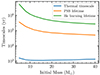 |
Fig. 3. Variation of various timescales with initial mass at SMC metallicity. The blue line represents the thermal timescale, and the orange line represents the puffed-up stripped star (PSS) lifetime. As can be seen, the PSS lifetime is ∼10–100 times longer than the thermal timescale. It is closer to the Helium burning lifetime, represented by a green line. |
This figure illustrates that the PSS phase is 10–100 times longer than the thermal timescale and about 10% of the He burning lifetime. This is in agreement with El-Badry & Quataert (2021), who noted a similar ratio of timescales in the low-mass regime of models.
The reason why the star contracts following detachment from point E to G is due to the continuous loss of mass from the remaining hydrogen envelope that was left unstripped during the mass transfer. The timescale of contraction and the PSS phase is thus dictated by the rate at which the envelope mass Menv decreases. There are two processes that contribute. One is stellar winds that directly strip mass from the envelope. The other is H-shell burning, which gradually grows the mass of the core, reducing Menv. Perhaps somewhat surprisingly, we find it is the H-shell burning that is the dominant process reducing Menv for most initial primary masses (Fig. 4). At LMC (SMC) metallicity, the winds begin to dominate only above about 54 M⊙ (63 M⊙) for our particular set of assumptions.
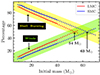 |
Fig. 4. Variation of the relative contribution of shell burning and winds to the hydrogen envelope depletion rate during the PSS phase, as a function of the initial donor mass. The yellow parts represent the contribution of shell burning, and the green region represents the contribution of winds. Red and blue lines represent LMC and SMC composition, respectively. The shell burning contributes more to the mass depletion of the envelope than the winds. The lines are extrapolated (dotted) to see the extent to which shell burning dominates. In the case of LMC, it is ∼54 M⊙, and in the case of SMC, it is 63 M⊙. Above this limit, the winds start to dominate the mass depletion of the envelope. |
The reason why the PSS phase is a transitional stage that is short compared to the He burning lifetime is because the envelope layer left after the mass transfer is thin and gets depleted. Had there been more envelope left after the mass transfer, the contraction PSS phase would have lasted longer. This is the case, for instance, in the high-semiconvection low-metallicity models of Klencki et al. (2022), where often ∼25 − 40% of the initial envelope remains unstripped and the star never contracts to the hot stripped-star stage, with the PSS phase lasting for the entire He burning lifetime. More massive residual envelopes are usually also more H-rich as a result of H/He gradients (Schootemeijer et al. 2019; Klencki et al. 2020; Kaiser et al. 2020; Higgins & Vink 2020), depleting the rate at which H-shell burning grows the He core mass and reduced Menv. To test this and further illustrate this point, we undertake an experiment. We initiate by evolving a binary system until the end of mass transfer. We then stop the evolution of the binary model, extract the donor star, switch off stellar winds, and let the stripped donor evolve further without any wind mass loss. In another experiment, we disable any composition changes due to nuclear burning instead of switching off the winds. The results are shown in Fig. 5 for the same 16 M⊙ example with LMC composition. In the illustrative model presented in Fig. 1, the duration of the phase characterised by a puffed-up stripped star is approximately 0.058 Myr. In contrast, in the scenario where the winds were deactivated, this duration extends to about 0.078 Myr. On the other hand, turning off compositional changes results in an extended period of approximately 0.27 Myr for the PSS phase. This example illustrates that by lowering the envelope depletion rate, we prolong the PSS lifetime and slow down the contraction. In the same time, wind mass loss rate (which is an uncertain factor in stellar models) is subdominant compared to H-shell burning. This suggests that the PSS lifetimes inferred in this work are not significantly affected by uncertainties in the wind mass loss rate of stripped stars (with the exception of very high masses).
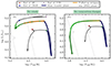 |
Fig. 5. Evolution of 16 M⊙ star in LMC composition considering no winds (left) and no composition changes (right). The colours and labels are the same as that of Fig. 1. For 16 M⊙, the winds play a subdominant role in stripping the envelope, and completely switching them off only prolongs the PSS phase by ∼1.3 times. On the other hand, in the hypothetical scenario with no composition changes due to burning (in particular H shell burning), the PSS phase would be much longer, by ∼4.7 times, illustrating the key role of shell burning in determining the evolution through the PSS phase. The green dots appear so close in the right plot, showing that the contraction happens very slowly as compared to the default scenario. |
3.3. Stellar tracks
In Fig. 6, we present HR diagrams from stellar masses ranging from 5 M⊙ to 40 M⊙ at LMC (Z = 0.4 Z⊙ = 0.0068) metallicity. The tracks show the evolution of the primary star from ZAMS to end to He burning. We mark the important phases in the evolutionary history as described in the legend.
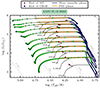 |
Fig. 6. Hertzsprung–Russel Diagram showing evolutionary tracks of the primary star in a binary system with initial masses 5, 6.5, 8, 10, 12, 16. 16.9, 20, 22, 26, 30 and 40 M⊙ at LMC metallicity. The blue lines represent the mass transfer phase, and the orange lines represent the puffed-up stripped star (PSS) phase. Red dots represent the terminal age main sequence (TAMS), and the blue squares represent the end of core Helium burning. The green dots are placed at intervals of 20 000 years starting from RLOF. The clustering of these dots towards the left shows that the star spends a long time in this phase. |
We find that the duration of the PSS phase depends on the initial mass and the metallicity. In Fig. 7 (left panel), we plot the lifetime of the puffed-up stripped star as a function of the initial mass (before mass transfer) and for various metallicities. Dashed lines represent numerical fits described by the relation:
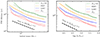 |
Fig. 7. Variation of puffed-up stripped star (PSS) lifetime (tPSS) with initial donor masses (left) and corresponding luminosity (right) at various metallicity (represented by various colours). Dashed lines represent fits for the corresponding data. The bold dashed line guides the eye to illustrate the steepness of the slopes. |
where TPSS = log(tPSS/yr), M = log(m/M⊙), and tPSS is the lifetime of puffed-up stripped star, m is the initial mass and Z is the metallicity. The values of co-efficient aij are given in Table 1. Notably, we find that the duration of the PSS phase tPSS can be well described by two independent factors, one related to mass and the other metallicity. It can be written as:

The relationship between the lifetime of a puffed-up stripped star, its mass, and its metallicity can be observed in Fig. 7. The decreasing slopes can be explained by considering two key mass- and metallicity-dependent factors: the amount of remaining (hydrogen) envelope mass after mass transfer and the rate of Menv depletion due to H shell burning and winds. Figure 8 illustrates these factors. When we compare models at a constant initial mass, we find that models with lower metallicity tend to retain a larger envelope mass after mass transfer, while models with higher metallicity lose more of their envelopes. Additionally, the rate of shell depletion decreases as we move to lower metallicities. Consequently, models with lower metallicity take a longer time to contract, and they naturally spend more time as PSSs. Conversely, models with higher initial mass, while retaining a larger envelope mass after mass transfer, experience a high rate of shell depletion. This leads to shorter contraction times and, subsequently, shorter PSS lifetimes when compared to models with lower initial mass.
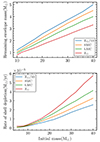 |
Fig. 8. Variation of the remaining envelope mass Menv (top) and average rate of Menv depletion (bottom) in stripped stars, plotted as a function of the initial mass. The combination of those two factors affects the duration of the PSS phase. |
A closer look at Fig. 6 suggests that the luminosity during the PSS phase remains almost constant. Therefore, we could use this luminosity as a proxy for the initial mass to rewrite the fits to tPSS as a function of the luminosity of the PSS phase. To this end, we also present corresponding fits following an equation similar to Eq. (2). Figure 7 (right panel) shows the lifetime of PSSs as a function of the PSS luminosity at different metallicities. The luminosity is represented by the average luminosity over the cool stripped star phase (time-weighted). The solid lines represent the lifetime of PSS stars from the binary MESA models. Dashed lines represent numerical fits described by the relation:
where l = log(L/L⊙), L is the corresponding luminosity, and Z is the metallicity. The co-efficient bij values are given in Table 2.
Similar to Eq. (2), this expression of time has two dependencies: luminosity and metallicity. It can be written as:

4. Discussion
4.1. How many puffed-up stripped stars can we expect in stellar populations?
The tracks computed in our work show that the lifetimes of puffed-up stripped stars are 10–100 times longer than just short thermal timescales that were sometimes assumed before, averaging 10% of the He burning lifetime and 1% of the total lifetime of a star. This is in line with the recent surge of detections of PSS binaries in optical spectroscopic surveys. In this section, we use our results to make an estimation of how many such binaries one can expect to find in low metallicity environments like the LMC and SMC. The detailed procedure for our estimation is explained below.
We assume galaxies with a constant star formation rate (SFR). The SFR is taken as 0.05 M⊙ yr−1 for SMC (Bolatto et al. 2011; Hagen et al. 2017; Rubele et al. 2015, 2018), 0.2 M⊙ yr−1 for LMC (Harris & Zaritsky 2009) and 2 M⊙ yr−1 for the Milky way (Chomiuk & Povich 2011; Licquia & Newman 2015). We are interested in finding stars in a specific phase in their evolution, one that lasts Δtevol and begins when the star is tage old. In our case, Δtevol corresponds to the puffed-up stripped star phase. The total mass of stars (Mstars) formed in that episode of star formation is then SFR(tage)×Δtevol, where SFR(tage) is the star formation rate in that galaxy tage years ago. If we assume a constant star formation rate, then that means that SFR is independent of tage. The Mstars can be calculated for any of the PSS duration values (Δtevol), assuming a star formation value and history of a particular galaxy. This would correspond to Nstars = Mstars/⟨Mstar⟩ stars, where Nstars is the number of stars and ⟨Mstar⟩ is the average mass of stars, given the Initial Mass Function (IMF). We consider the IMF from Kroupa (2002):
where α1 = 1.3 for M/M⊙ ∈ [0.08, 0.5] and α2 = α3 = 2.3 for M/M⊙ ∈ [0.5, 1.0] and [1.0, 150.0] respectively. We normalise ξ(M) to find the constants, and from the final value, we calculate ⟨Mstar⟩:
This gives us ⟨Mstar⟩ as 0.635.
To account for the lifetime of the puffed-up stripped stars derived in Eq. (2), we use mass bins at an interval of 2 solar masses ranging from 5 M⊙ to 40 M⊙. Δtevol corresponds to a particular mass bin. This means that we are only interested in what fraction of all stars (fM) formed during a star formation period that produced Nstars in a certain mass bin, for instance, which goes from M1 to M2. We integrate a normalised IMF from M1 to M2 to get fM. Nstars_of_interest = fM × Nstars gives us the number of stars (in singles, binaries, in triples) with the mass from the mass bin and formed at such a time period ago that right now we would see them as puffed-up stripped stars. We also assume that the IMF describes the distribution of primaries in multiple systems. So coupled with an assumption of an initial binary fraction of 100%, Nstars_of_interest roughly gives us the number of binary systems that formed with primaries in our mass bin, tage years ago, during a period of Δtevol years.
In this process, we have considered all binaries without any constraints on mass ratios or periods. However, throughout this work, we specifically consider case B binaries and, therefore, need to put a constraint on the mass ratios and orbital periods. To this end, we consider distribution functions for orbital periods (P) and mass ratios (q) following de Mink & Belczynski (2015). These distributions were motivated by the spectroscopic observations of massive stars by Sana et al. (2012). The distributions are:
![$$ \begin{aligned} f_P(\log P) \propto (\log P)^\pi , \, \mathrm{for} \log P \in \mathrm{[0.15, 5.5]} \end{aligned} $$](/articles/aa/full_html/2024/07/aa49065-23/aa49065-23-eq10.gif)
where π = 0.5
![$$ \begin{aligned} f_q(q) \propto q^\kappa , \, \mathrm{for} q \in \mathrm{[0.1, 1.0]} \end{aligned} $$](/articles/aa/full_html/2024/07/aa49065-23/aa49065-23-eq11.gif)
where κ = −0.1 ± 0.6 The range for log P is chosen from Fig. C.2 of Klencki et al. (2020) such that it corresponds to case B mass transfer evolution. For the LMC and SMC, we adopt identical ranges for orbital periods (log P) across all mass bins due to small variations within the considered mass range. For convective-envelope donors, this range falls between ∼2.69 to ∼3.47, and for radiative-envelope donors, this range falls between ∼0.47 to ∼2.69 (for LMC metallicity). However, for solar metallicity, we employ distinct ranges of orbital periods for each mass bin, reflecting the considerable variability (eg. the lower range of log P itself varies from ∼0.6 to ∼3.3) observed in this context. Here, we focus on stable mass transfer evolution, meaning we want to exclude cases that are likely to experience a common-envelope phase. For simplicity, we assume that mass transfer remains stable for q > 0.33 (radiative-envelope donors) or q > 0.66 (convective-envelope donors).
Using this method and the underlying assumptions, we could estimate the number of puffed-up stripped stars of different masses and luminosities in the environments of the SMC and LMC. Figure 9 shows the results obtained. Our results indicate ∼100 stars in the SMC, ∼280 stars in the LMC and ∼1500 stars in the Milky Way, which are puffed-up stripped stars in the luminosity range log(L/L⊙) > 3.7. As can be seen, such stars are more common in the lower (initial) mass and luminosity regime. This would explain the increasing number of low-mass stars observed compared to their massive counterparts. Further, as PSS binaries are expected to overlap with MS stars, we compare their expected numbers to the number of all MS stars, taking the SMC environment as an example and following Schootemeijer et al. 2021, see their Fig. 3). The authors count ∼732 stars in the luminosity (log(L/L⊙))(log(L/L⊙)) range 4.6–4.8, most of which are MS stars. Our estimation of PSS yields ∼4 stars in that range, which is about 0.54% of MS stars. Similarly, in the luminosity (log(L/L⊙)) ranges 4.8–5.1 and 5.1–5.3, the corresponding fractions are 0.61% and 0.66%, respectively. We conclude that PS stars may constitute about 0.5–0.7% of the MS population. This may be expected given that the PSS lifetime is about 1–2% of the entire stellar lifetime and that not all the binaries will evolve through stable mass transfer and experience a PSS phase. Although estimated for the SMC, we expect this fraction to be similar in the LMC and the Milky Way environments. This implies that there are still tens of PSS stars disguised as MS stars in the current and upcoming optical surveys.
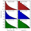 |
Fig. 9. Estimates of the number of PS stars that can be found at different mass ranges (left) and different luminosity ranges(right) at SMC (upper) and LMC (middle) and solar (lower) metallicities. Values above the bars in the upper right panel show the percentage of puffed-up stripped stars relative to the number of all stars in that luminosity bin, most of which are MS, based on Schootemeijer et al. (2021). |
4.2. The duration of the PSS phase
The transition between ‘puffed-up’ and ‘hot and compact’ stripped stars is not easily defined. A useful distinction between different types of stripped-star binaries can be made based on their spectral features, varying as a function of the stripped-star surface temperature and its relative contribution to the total flux of the binary (Drout et al. 2023; Götberg et al. 2023). In this work, our goal was to adopt an approximate criterion sufficiently robust to provide at least an order-of-magnitude estimate for the number of PSS in a stellar population. To this end, we assumed that the PSS begins at the end of mass transfer and continues until the effective temperature of the stripped star becomes hotter than its ZAMS temperature plus 0.1 dex. This was motivated by focusing on those stripped stars that in the HR diagram overlap with the MS and could, therefore, be hiding among the ‘normal’ OB stars. Finding candidates for post-interaction systems containing such PS stars could be done by selecting OB stars that stand out in terms of their low surface gravity (or high luminosity-to-mass ratio, if the luminosity is known) and high nitrogen enrichment while also usually being slow rotators (Klencki et al. 2022).
In practice, the position of the binary in the HR diagram and the prominence of those spectral stripped-star features will depend on the relative contribution of both binary components to the combined spectra. An extensive discussion of the observability of PS star binaries would require exploring a suite of composite combined spectra for a range of different companions, which is beyond the scope of this paper. Instead, we check how the duration of the observable PSS phase would vary, assuming that it lasts for as long as the relative flux of the PS star to its companion in the F450W optical filter of the HST WFPC2 camera is above a certain threshold. For this experiment, we assume the HR diagram position of the companion is either that of the primary at TAMS or that of the primary at 75% of the MS lifetime (red and green respectively in Fig. 10). The figure illustrates that our default criteria (solid black line) yield PSS lifetimes are comparable to those assuming fstripped/fcompanion > 1 for companions at 0.75 of the MS or to fstripped/fcompanion > 0.5 for companions at the TAMS luminosity of the primary. More luminous companions are also possible: assuming a companion brighter by another factor of 0.2 dex with respect to primary TAMS (such that its bolometric luminosity is similar to that of a stripped star) would mean that the dotted lines in Fig. 10 correspond to fstripped/fcompanion > 0.3. However, even with a companion ∼3 times brighter than the PS star, it may still be possible to detect the stripped star characteristics in the combined spectra if the companion is fast rotating and its lines broadened, as is usually the case in post-interaction binaries detected to date. Thus, we expect our default criterion for locating the PS phase to be accurate enough for the purpose of order-of-magnitude estimation of the number of PS star binaries in stellar populations. Notably, such systems may also ultimately be identified and spectrally disentangled in cases when it is the companion that strongly outshines the stripped star, provided that the stripped star contributes at least ∼10 − 20% of the combined flux (Saracino et al. 2023).
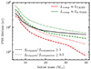 |
Fig. 10. Duration of the puffed-up stripped star (PSS) stage when the flux of the PS star in the optical F450W filter is at least equal (dashed) or half (dotted) the flux of its companion, for two assumed companion luminosities (red and green, see text), compared to our default PSS stage criteria based on the HR diagram position (black, solid). These are calculated at SMC metallicity. |
4.3. Puffed-up stripped stars after core He depletion
After the PSS phase, the star enters the phase of core He burning. Due to the energy produced by He burning, the contraction is halted. At the end of core-He burning, upon central He depletion, the carbon-oxygen core begins to contract again, and the remaining envelope expands. In some cases, this leads to a substantial expansion of the entire star again (even up to hundreds of R⊙), such that the star begins to appear as a PS star again (Laplace et al. 2020). We follow the behaviour of models until the end of central C burning, after which point there is generally not enough time for any significant change in the radius of the star before the core collapses.
The post-core He burning expansion takes place in all our models for stars with initial masses below ∼10 M⊙. Going to higher masses, the degree of late expansion becomes metallicity dependent: high metallicity massive stars lose too much H/He envelope during core-He burning, such that they remain compact until the core collapses. For example, in our representative stars of 16 M⊙ (Fig. 1), the star with LMC metallicity expands up to ∼1 R⊙; whereas the star with lower metallicity (Z⊙/10) expands upto ∼100 R⊙. The metallicity effects on post-core He burning expansion are discussed in detail by Laplace et al. (2020).
As a result of this expansion, stars exhibiting similar characteristics to puffed-up stripped stars are observable in the HR diagram. Notably, PS stars at this expanding stage are more luminous compared to PS stars contracting after the end of mass transfer, having thus even higher L/M ratio (which might be used to distinguish expanding PS stars from the contracting ones), given sufficiently accurate determination of atmospheric parameters. These particular stars were omitted from our star count estimation, and our lifetimes are for the contracting ones only. This is justified because the duration of the expansion phase (which coincides with the temperature range of the PSS phase) is notably shorter (by a factor of ∼10), making it considerably challenging to detect. For example, in our 16 M⊙ model at Z⊙/10 metallicty (right panel of Fig. 1), the time spent in that phase (considering the phase lasts from about H to I) is 12.46 kyr compared to our PSS lifetime of 126.55 kyr.
4.4. Factors affecting the contraction time
The computed PSS lifetimes and the estimated numbers of PSS binaries expected in a stellar population are affected by several uncertainties. Here we summarise the expected impact of the main uncertainties (winds, internal mixing, and the single choice of orbital period and mass ratio), with a more detailed investigation given in the appendix.
To estimate the number of PSS binaries in the SMC and LMC environments (Sect. 4.1), we relied on PSS lifetimes derived from our grids of binary-evolution models. Those models were computed for a single choice of the orbital period (Pini = 70 days) and mass ratio (qini = 0.6), whereas in a real population binaries with other periods and mass ratios clearly exist. In Appendix A we explore how the PSS lifetime changes for varying Pini and qini (A.2 and A.4). In general, longer periods and more equal mass ratios lead to more of the envelope being unstripped during the mass transfer and, consequently, to longer PSS lifetimes. In the case of mass ratio, the effect is quite small, with the PSS lifetime changing by less than 15% for qini ranging from 0.4 to 1.0. In the case of the varying orbital period, the effect is more significant. We find that in the range of periods from ∼10 to ∼1000 days (i.e., approximately the entire case B mass transfer range), the PSS lifetime varies by up to ∼2.5 times with respect to our reference model at 70 days, increasing with Pini. As most of the parameter space for case B mass transfer are periods Pini > 70 d, the estimated number of PSS stars in Sect. 4.1 (based only case B evolution) is thus likely underestimated by a factor ∼1 − 2 due to our orbital period choice. We also note that the PSS lifetimes originating from case A mass transfer are a factor of a few shorter than those from case B evolution.
In terms of uncertainties due to input physics of stellar models, the evolution of stripped stars is particularly sensitive to the assumed wind mass-loss rates as well as the efficiency of internal chemical mixing. Winds directly affect how quickly the residual unstripped envelope is depleted, which is what determines the PSS lifetime. In Appendix B we and Fig. B.1 we show that enhancing the winds by a factor of 10 leads to PSS lifetimes shorter by a factor of ∼2.5 (∼5) for a stripped star originating from a 16 M⊙ (30 M⊙), respectively. The mass dependence comes from the fact that the lower the mass, the less significant the contribution of winds relative to H-shell burning in depleting the H-rich envelope. Decreasing the strength of winds with respect to our reference model has minimal effect on the PSS lifetime unless very high mass stars are considered (see Sect. 3.2 and Fig. 4). Internal mixing, on the other hand, plays a role because it affects the chemical gradient of bottom envelope layers of giants, which in turn has an impact on when the binary detaches from mass transfer and the residual amount of unstripped envelope (Schootemeijer et al. 2019; Klencki et al. 2020; Kaiser et al. 2020; Higgins & Vink 2020). In addition, the extend of core-overshooting and semiconvective mixing has strong effect on the post-MS expansion of massive low-metallicity stars (Langer et al. 1985; Langer 1991; Langer & Maeder 1995; Maeder & Meynet 2001), which in turn can sometimes lead to the phenomenon of partial-envelope stripping (Klencki et al. 2022): case B mass transfer from core-He burning giants leading to residual unstripped envelopes so massive, that the stripped star remains puffed-up and never contracts to become UV-bright and compact. Such cases would lead to PSS lifetimes equaling core-He burning lifetimes, i.e., ∼10 times longer than our reference models, see Appendix C and Fig. C.1. Such long-lived PSS are restricted to high masses ≳15 − 20 M⊙ (depending on overshooting) and do not affect the core of our analysis.
5. Summary and conclusions
In this paper, we have studied the post-mass transfer evolution of stars that have undergone stripping in binary systems. We put specific focus on understanding puffed-up stripped stars (PSS), i.e., stars that have lost most of their hydrogen envelope but the remaining envelope is puffed-up, such that the stripped star is as large and cool as normal MS stars or event post-MS giants. To this end, we employed the stellar evolution code MESA to calculate grids of binary models at four different metallicities (solar, LMC, SMC and 1/10th solar) encompassing a wide range of initial primary masses (from 5 M⊙ to 40 M⊙). Our principal emphasis revolved around the post-mass transfer evolution of the primary star. For simplicity, the secondary star was treated as a point mass. For most of the models, we maintained a consistent set of parameters, initiating the binary systems with an initial orbital period Pini = 70 days and an initial mass ratio qini = 0.6. However, we also conducted exploratory investigations into how variations in Pini, qini, wind mass loss, and semiconvective mixing might affect the outcomes in select cases. Our conclusions can be summarised as follows.
-
After the end of mass transfer, the primary star (mass loser) initiates a process of contraction to eventually become a hot and compact (≲1 R⊙) stripped star, observable in UV. During contraction, it is observable as a much cooler and larger puffed-up stripped (PS) star. The contraction is a transitory phase but is much longer than the thermal timescale of the primary (by ∼2 orders of magnitude), with PSS lifetimes typically equalling about 1% of the total stellar lifetime.
-
Thermal equilibrium is restored very soon after the end of mass transfer and maintained throughout the PSS phase, with negligible contribution from contraction to the total energy budget of the star ≲1% (Fig. 2). The main energy source in PS stars is H shell burning occurring in the residual envelope, unstripped during the mass transfer.
-
The reason why stripped stars continuously contract after the end of mass transfer is because they continue to lose mass from their residual hydrogen envelope. PS star lifetimes and the pace of contraction are determined by how quickly the residual envelope is depleted. The two agents at play are stellar winds that directly strip the envelope, and H-shell burning, which grows the He core at the expense of the H envelope. We find that H-shell burning is the dominant effect for initial masses even up to ≲50 M⊙, see Fig. 4 (e.g., H-shell burning is responsible for ≈90% of the envelope mass loss in PS stars from ∼10 to 15 M⊙ primaries at LMC metallicity).
-
Uncertainties in wind-mass loss rates of stripped stars have a non-trivial effect on the duration of the PSS phase. Our default assumption of winds follows Nugis & Lamers (2000). Assuming winds stronger by a factor of 10× leads to PSS phase shorter by a factor of ∼2.5 (∼3.2) for the initial primary mass 16 M⊙ (30 M⊙), respectively. However, assuming weaker winds have a much smaller effect on the PS lifetimes (Fig. B.1): this is because most of the residual envelope is depleted through H-shell burning anyway.
-
The duration of the PSS phase depends on the remaining (hydrogen) envelope mass after mass transfer and the rate of envelope mass depletion. The duration decreases with increasing mass (at constant metallicity) due to the high rate of envelope mass depletion. With decreasing metallicity (at constant initial mass), the PSS lifetimes increase thanks to higher remaining envelope masses, prolonging the contraction. A similar effect can be observed with orbital periods, where the PSS lifetime increases with larger orbital periods and also with initial mass ratio, where a greater mass ratio leads to longer PSS duration.
-
Based on a simple population model, we predicted that about ∼100 (in the SMC), nearly ∼280 (in the LMC) and about ∼1500 (in the Milky Way) PS stars exist in the luminosity range log(L/L⊙) > 3.7 (corresponding to the initial mass range 5–40 M⊙). We estimate that 0.5–0.7% of all the stars in that luminosity range are, in fact, PS stars in post-interaction binaries, suggesting that many such systems are awaiting detection. We discuss several uncertainties and simplifications of the above estimate, deeming it likely robust within the factor of ∼5.
Acknowledgments
We thank the anonymous referee for the useful comments and suggestions. It is a pleasure to acknowledge valuable inputs and discussions with Julia Bodensteiner. DD would like to thank Projjwal Banerjee for his advice and comments regarding the paper. JK acknowledges support from an ESO Fellowship.
References
- Baraffe, I., & El Eid, M. F. 1991, A&A, 245, 548 [NASA ADS] [Google Scholar]
- Bodensteiner, J., Shenar, T., Mahy, L., et al. 2020, A&A, 641, A43 [NASA ADS] [CrossRef] [EDP Sciences] [Google Scholar]
- Böhm-Vitense, E. 1958, Z. Astrophys., 46, 108 [Google Scholar]
- Bolatto, A. D., Leroy, A. K., Jameson, K., et al. 2011, ApJ, 741, 12 [CrossRef] [Google Scholar]
- Brott, I., de Mink, S. E., Cantiello, M., et al. 2011, A&A, 530, A115 [NASA ADS] [CrossRef] [EDP Sciences] [Google Scholar]
- Brunish, W. M., & Truran, J. W. 1982, ApJS, 49, 447 [NASA ADS] [CrossRef] [Google Scholar]
- Buchler, J. R., & Yueh, W. R. 1976, ApJ, 210, 440 [NASA ADS] [CrossRef] [Google Scholar]
- Cassisi, S., Potekhin, A. Y., Pietrinferni, A., Catelan, M., & Salaris, M. 2007, ApJ, 661, 1094 [NASA ADS] [CrossRef] [Google Scholar]
- Chomiuk, L., & Povich, M. S. 2011, AJ, 142, 197 [Google Scholar]
- De Loore, C., & De Greve, J. P. 1992, A&AS, 94, 453 [NASA ADS] [Google Scholar]
- de Mink, S. E., & Belczynski, K. 2015, ApJ, 814, 58 [Google Scholar]
- de Mink, S. E., Pols, O. R., & Yoon, S. C. 2008, in First Stars III, eds. B. W. O’Shea, & A. Heger, AIP Conf. Ser., 990, 230 [Google Scholar]
- Drout, M. R., Götberg, Y., Ludwig, B. A., et al. 2023, Science, 382, 1287 [NASA ADS] [CrossRef] [Google Scholar]
- El-Badry, K., & Burdge, K. B. 2022, MNRAS, 511, 24 [NASA ADS] [CrossRef] [Google Scholar]
- El-Badry, K., & Quataert, E. 2021, MNRAS, 502, 3436 [NASA ADS] [CrossRef] [Google Scholar]
- Eldridge, J. J., Izzard, R. G., & Tout, C. A. 2008, MNRAS, 384, 1109 [Google Scholar]
- Eldridge, J. J., Fraser, M., Smartt, S. J., Maund, J. R., & Crockett, R. M. 2013, MNRAS, 436, 774 [NASA ADS] [CrossRef] [Google Scholar]
- Eldridge, J. J., Stanway, E. R., Breivik, K., et al. 2020, MNRAS, 495, 2786 [Google Scholar]
- Farrell, E., Groh, J. H., Meynet, G., & Eldridge, J. J. 2022, MNRAS, 512, 4116 [NASA ADS] [CrossRef] [Google Scholar]
- Georgy, C., Ekström, S., Eggenberger, P., et al. 2013, A&A, 558, A103 [NASA ADS] [CrossRef] [EDP Sciences] [Google Scholar]
- Georgy, C., Granada, A., Ekström, S., et al. 2014, A&A, 566, A21 [NASA ADS] [CrossRef] [EDP Sciences] [Google Scholar]
- Gies, D. R., Bagnuolo, W. G. Jr, Ferrara, E. C., et al. 1998, ApJ, 493, 440 [NASA ADS] [CrossRef] [Google Scholar]
- Glebbeek, E., Gaburov, E., de Mink, S. E., Pols, O. R., & Portegies Zwart, S. F. 2009, A&A, 497, 255 [NASA ADS] [CrossRef] [EDP Sciences] [Google Scholar]
- Götberg, Y., de Mink, S. E., & Groh, J. H. 2017, A&A, 608, A11 [NASA ADS] [CrossRef] [EDP Sciences] [Google Scholar]
- Götberg, Y., de Mink, S. E., Groh, J. H., et al. 2018, A&A, 615, A78 [NASA ADS] [CrossRef] [EDP Sciences] [Google Scholar]
- Götberg, Y., de Mink, S. E., Groh, J. H., Leitherer, C., & Norman, C. 2019, A&A, 629, A134 [NASA ADS] [CrossRef] [EDP Sciences] [Google Scholar]
- Götberg, Y., de Mink, S. E., McQuinn, M., et al. 2020a, A&A, 634, A134 [EDP Sciences] [Google Scholar]
- Götberg, Y., Korol, V., Lamberts, A., et al. 2020b, ApJ, 904, 56 [CrossRef] [Google Scholar]
- Götberg, Y., Drout, M. R., Ji, A. P., et al. 2023, ApJ, 959, 125 [CrossRef] [Google Scholar]
- Grevesse, N., & Sauval, A. J. 1998, Space Sci. Rev., 85, 161 [Google Scholar]
- Grevesse, N., Noels, A., & Sauval, A. J. 1996, in Cosmic Abundances, eds. S. S. Holt, & G. Sonneborn, ASP Conf. Ser., 99, 117 [Google Scholar]
- Groh, J. H., Ekström, S., Georgy, C., et al. 2019, A&A, 627, A24 [NASA ADS] [CrossRef] [EDP Sciences] [Google Scholar]
- Groh, J. H., Oliveira, A. S., & Steiner, J. E. 2008, A&A, 485, 245 [NASA ADS] [CrossRef] [EDP Sciences] [Google Scholar]
- Hagen, L. M. Z., Siegel, M. H., Hoversten, E. A., et al. 2017, MNRAS, 466, 4540 [NASA ADS] [Google Scholar]
- Harris, J., & Zaritsky, D. 2009, AJ, 138, 1243 [NASA ADS] [CrossRef] [Google Scholar]
- Herwig, F. 2000, A&A, 360, 952 [NASA ADS] [Google Scholar]
- Higgins, E. R., & Vink, J. S. 2020, A&A, 635, A175 [NASA ADS] [CrossRef] [EDP Sciences] [Google Scholar]
- Hut, P. 1981, A&A, 99, 126 [NASA ADS] [Google Scholar]
- Iglesias, C. A., & Rogers, F. J. 1993, ApJ, 412, 752 [Google Scholar]
- Iglesias, C. A., & Rogers, F. J. 1996, ApJ, 464, 943 [NASA ADS] [CrossRef] [Google Scholar]
- Irrgang, A., Przybilla, N., & Meynet, G. 2022, Nat. Astron., 6, 1414 [NASA ADS] [CrossRef] [Google Scholar]
- Ivanova, N. 2011, ApJ, 730, 76 [Google Scholar]
- Jermyn, A. S., Bauer, E. B., Schwab, J., et al. 2023, ApJS, 265, 15 [NASA ADS] [CrossRef] [Google Scholar]
- Kaiser, E. A., Hirschi, R., Arnett, W. D., et al. 2020, MNRAS, 496, 1967 [Google Scholar]
- Kalogera, V. 1997, PASP, 109, 1394 [NASA ADS] [CrossRef] [Google Scholar]
- Kalogera, V., Belczynski, K., Kim, C., O’Shaughnessy, R., & Willems, B. 2007, Phys. Rep., 442, 75 [Google Scholar]
- Kippenhahn, R. 1969, A&A, 3, 83 [NASA ADS] [Google Scholar]
- Kippenhahn, R., & Weigert, A. 1967, Z. Astrophys., 65, 251 [NASA ADS] [Google Scholar]
- Kippenhahn, R., Ruschenplatt, G., & Thomas, H. C. 1980, A&A, 91, 175 [Google Scholar]
- Klencki, J., Nelemans, G., Istrate, A. G., & Pols, O. 2020, A&A, 638, A55 [NASA ADS] [CrossRef] [EDP Sciences] [Google Scholar]
- Klencki, J., Istrate, A., Nelemans, G., & Pols, O. 2022, A&A, 662, A56 [NASA ADS] [CrossRef] [EDP Sciences] [Google Scholar]
- Kolb, U., & Ritter, H. 1990, A&A, 236, 385 [NASA ADS] [Google Scholar]
- Kroupa, P. 2002, Science, 295, 82 [Google Scholar]
- Langer, N. 1991, A&A, 252, 669 [NASA ADS] [Google Scholar]
- Langer, N., & Maeder, A. 1995, A&A, 295, 685 [NASA ADS] [Google Scholar]
- Langer, N., El Eid, M. F., & Fricke, K. J. 1985, A&A, 145, 179 [NASA ADS] [Google Scholar]
- Laplace, E., Götberg, Y., de Mink, S. E., Justham, S., & Farmer, R. 2020, A&A, 637, A6 [NASA ADS] [CrossRef] [EDP Sciences] [Google Scholar]
- Laplace, E., Justham, S., Renzo, M., et al. 2021, A&A, 656, A58 [NASA ADS] [CrossRef] [EDP Sciences] [Google Scholar]
- Licquia, T. C., & Newman, J. A. 2015, ApJ, 806, 96 [NASA ADS] [CrossRef] [Google Scholar]
- Liu, J., Zhang, H., Howard, A. W., et al. 2019, Nature, 575, 618 [Google Scholar]
- Maeder, A., & Meynet, G. 2001, A&A, 373, 555 [NASA ADS] [CrossRef] [EDP Sciences] [Google Scholar]
- Moe, M., & Di Stefano, R. 2017, ApJS, 230, 15 [Google Scholar]
- Nugis, T., & Lamers, H. J. G. L. M. 2000, A&A, 360, 227 [NASA ADS] [Google Scholar]
- Paczyński, B. 1967, Acta Astron., 17, 355 [NASA ADS] [Google Scholar]
- Paxton, B., Bildsten, L., Dotter, A., et al. 2011, ApJS, 192, 3 [Google Scholar]
- Paxton, B., Cantiello, M., Arras, P., et al. 2013, ApJS, 208, 4 [Google Scholar]
- Paxton, B., Marchant, P., Schwab, J., et al. 2015, ApJS, 220, 15 [Google Scholar]
- Paxton, B., Schwab, J., Bauer, E. B., et al. 2018, ApJS, 234, 34 [NASA ADS] [CrossRef] [Google Scholar]
- Paxton, B., Smolec, R., Schwab, J., et al. 2019, ApJS, 243, 10 [Google Scholar]
- Peters, G. J., Pewett, T. D., Gies, D. R., Touhami, Y. N., & Grundstrom, E. D. 2013, ApJ, 765, 2 [Google Scholar]
- Petrovic, J., Langer, N., & van der Hucht, K. A. 2005, A&A, 435, 1013 [NASA ADS] [CrossRef] [EDP Sciences] [Google Scholar]
- Podsiadlowski, P., Joss, P. C., & Hsu, J. J. L. 1992, ApJ, 391, 246 [Google Scholar]
- Ramachandran, V., Klencki, J., Sander, A. A. C., et al. 2023, A&A, 674, L12 [NASA ADS] [CrossRef] [EDP Sciences] [Google Scholar]
- Rivinius, T., Baade, D., Hadrava, P., Heida, M., & Klement, R. 2020, A&A, 637, L3 [NASA ADS] [CrossRef] [EDP Sciences] [Google Scholar]
- Rubele, S., Girardi, L., Kerber, L., et al. 2015, MNRAS, 449, 639 [NASA ADS] [CrossRef] [Google Scholar]
- Rubele, S., Pastorelli, G., Girardi, L., et al. 2018, MNRAS, 478, 5017 [NASA ADS] [CrossRef] [Google Scholar]
- Sana, H., de Mink, S. E., de Koter, A., et al. 2012, Science, 337, 444 [Google Scholar]
- Sana, H., Le Bouquin, J. B., Lacour, S., et al. 2014, ApJS, 215, 15 [Google Scholar]
- Sander, A. A. C., & Vink, J. S. 2020, MNRAS, 499, 873 [Google Scholar]
- Saracino, S., Kamann, S., Guarcello, M. G., et al. 2022, MNRAS, 511, 2914 [NASA ADS] [CrossRef] [Google Scholar]
- Saracino, S., Shenar, T., Kamann, S., et al. 2023, MNRAS, 521, 3162 [NASA ADS] [CrossRef] [Google Scholar]
- Schootemeijer, A., Langer, N., Grin, N. J., & Wang, C. 2019, A&A, 625, A132 [NASA ADS] [CrossRef] [EDP Sciences] [Google Scholar]
- Schootemeijer, A., Langer, N., Lennon, D., et al. 2021, A&A, 646, A106 [NASA ADS] [CrossRef] [EDP Sciences] [Google Scholar]
- Shao, Y., & Li, X.-D. 2021, ApJ, 908, 67 [NASA ADS] [CrossRef] [Google Scholar]
- Shenar, T., Bodensteiner, J., Abdul-Masih, M., et al. 2020a, A&A, 639, L6 [EDP Sciences] [Google Scholar]
- Shenar, T., Gilkis, A., Vink, J. S., Sana, H., & Sander, A. A. C. 2020b, A&A, 634, A79 [NASA ADS] [CrossRef] [EDP Sciences] [Google Scholar]
- Shenar, T., Wade, G. A., Marchant, P., et al. 2023, Science, 381, 761 [NASA ADS] [CrossRef] [Google Scholar]
- Smith, N., Li, W., Filippenko, A. V., & Chornock, R. 2011, MNRAS, 412, 1522 [NASA ADS] [CrossRef] [Google Scholar]
- Steiner, J. E., & Oliveira, A. S. 2005, A&A, 444, 895 [NASA ADS] [CrossRef] [EDP Sciences] [Google Scholar]
- Tang, J., Bressan, A., Rosenfield, P., et al. 2014, MNRAS, 445, 4287 [NASA ADS] [CrossRef] [Google Scholar]
- van den Heuvel, E. P. J. 1975, ApJ, 198, L109 [NASA ADS] [CrossRef] [Google Scholar]
- Vanbeveren, D. 1991, A&A, 252, 159 [NASA ADS] [Google Scholar]
- Vanbeveren, D., De Loore, C., & Van Rensbergen, W. 1998, A&A Rev., 9, 63 [NASA ADS] [CrossRef] [Google Scholar]
- Vartanyan, D., Laplace, E., Renzo, M., et al. 2021, ApJ, 916, L5 [NASA ADS] [CrossRef] [Google Scholar]
- Villaseñor, J. I., Lennon, D. J., Picco, A., et al. 2023, MNRAS, 525, 5121 [CrossRef] [Google Scholar]
- Vink, J. S., & de Koter, A. 2005, A&A, 442, 587 [NASA ADS] [CrossRef] [EDP Sciences] [Google Scholar]
- Vink, J. S., de Koter, A., & Lamers, H. J. G. L. M. 2001, A&A, 369, 574 [NASA ADS] [CrossRef] [EDP Sciences] [Google Scholar]
- Wang, L., Gies, D. R., & Peters, G. J. 2017, ApJ, 843, 60 [Google Scholar]
- Wang, L., Gies, D. R., & Peters, G. J. 2018, ApJ, 853, 156 [Google Scholar]
- Wang, L., Gies, D. R., Peters, G. J., et al. 2021, AJ, 161, 248 [Google Scholar]
- Wellstein, S., Langer, N., & Braun, H. 2001, A&A, 369, 939 [NASA ADS] [CrossRef] [EDP Sciences] [Google Scholar]
- Yoon, S.-C. 2015, PASA, 32, e015 [NASA ADS] [CrossRef] [Google Scholar]
- Yoon, S.-C., Dessart, L., & Clocchiatti, A. 2017, ApJ, 840, 10 [NASA ADS] [CrossRef] [Google Scholar]
Appendix A: Effect of orbital period and mass ratio on the lifetime of a puffed-up stripped star
In this section, we investigate how the orbital period and mass ratio influence the post-interaction contraction, thereby the time period of the bloated stripped star phase. We take models with initial stellar mass 16 M⊙ and 30 M⊙ at LMC metallicity (Z = 0.0068) and vary their orbital periods and mass ratios.
A.1. Orbital periods
In A.1, we have plotted the full stellar evolution tracks at various orbital periods ranging from 1 day to 100 days. The models with periods 1 day and 5 days undergo mass transfer still when in the main sequence (case A). Since our focus is on case B mass transfer, we do not consider them in our discussion.
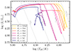 |
Fig. A.1. Evolutionary tracks of 16M⊙ models at LMC metallicity (with varied initial orbital periods (Pini)) on the HR diagrams. Various colours indicate the various values of Pini described in the legend. |
Fig. A.2 shows the variation of the puffed-up stripped star (PSS) lifetime with various orbital periods. It can be seen that the PSS lifetime increases with increasing orbital periods. This happens because, for longer orbital periods, we have wider separation and, thus bigger Roche lobes. With a larger Roche lobe, the primary star detaches from its companion sooner compared to a scenario with a smaller Roche lobe. Consequently, stars with longer orbital periods experience less efficient mass stripping, retaining more of their envelope mass. As explained in Section 3.2, the envelope mass of a star is a pivotal factor in determining the duration of its contraction phase. In this context, the increased envelope mass for stars with longer orbital periods leads to a slower contraction process. This phenomenon contributes to the observed extended lifetime of puffed-up stripped stars in such systems.
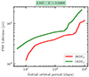 |
Fig. A.2. Variation of initial orbital period Pini with puffed-up stripped star (PSS) lifetime of 16 and 30 M⊙ models at LMC metallicity. |
A.2. Mass ratio
Fig. A.3 shows stellar tracks at various mass ratios (q = M2/M1) ranging from 0.4 to 1.0. Our default mass ratio used is 0.6. We consider all the models here as all of them undergo case B mass transfer
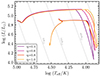 |
Fig. A.3. Evolutionary tracks of 16M⊙ models at LMC metallicity (with varied initial mass ratio (qini)) on the HR diagram. Various colours indicate various mass ratios described in the legend. |
The influence of mass ratio on the orbital period is illustrated in Fig. A.4. An increase in mass ratios correlates with an extended lifetime of BSS. This phenomenon arises from the transfer of mass from a more massive star to a less massive companion. Consequently, the orbital separation decreases to conserve angular momentum. The mass of the primary star decreased, reaching a critical point where the mass ratio undergoes reversal, leading to an increase in orbital separation. As the mass ratio approaches unity, the orbit could not shrink at all due to the rapid reversal of the mass ratio, resulting in a substantial separation between the stars. This expansive separation gives rise to a larger Roche lobe. As explained in the previous section, a larger Roche lobe contributes to inefficient mass stripping, allowing the retention of more envelope mass, resulting in longer contraction time
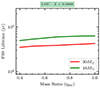 |
Fig. A.4. Variation of initial mass ratio (qini) with puffed-up stripped star (PSS) lifetime of 16 and 30 M⊙ models at LMC metallicity. |
Appendix B: Effect of winds on the lifetime of a puffed-up stripped star
In the previous section, we discussed how the primary factor influencing the contraction of a puffed-up stripped star is the process of shell hydrogen burning. However, above a certain mass, stellar winds also play a significant role in determining the rate of contraction. This limit is different for different metallicities. For SMC, it is 54 M⊙, and for LMC, it is 63 M⊙. Above this limit, winds can have an impact on the overall lifetime of the PSS.
There is ongoing debate and uncertainty surrounding the mass-loss rates of stripped stars (Yoon 2015; Götberg et al. 2017, 2018). These rates are generally calculated from the Wolf-Rayet scheme of Nugis & Lamers (2000). The effect of the winds is somewhat less for lower metallicity (Vink & de Koter 2005). This relation with metallicity exerts an impact on the mass of the residual H envelope. In the context of puffed-up stripped stars, it is important to recognise that the lifetime of a puffed-up stripped star depends on how much envelope mass remains and the nuclear burning rate of the shell. The amount of mass that can be carried away by these winds also plays a role in shaping the evolution and, by extension, its lifetime.
We conducted experiments involving variations in the wind mass-loss rates to investigate their impact on the PSS lifetime. Figure B.1 illustrates the relationship between different wind rates and the PSS lifetime. Our findings indicate that as the wind mass-loss rates increase, the PSS lifetime decreases. This phenomenon occurs because more vigorous winds result in a less massive envelope surrounding the star, which in turn depletes more rapidly than it would with a larger envelope.
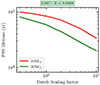 |
Fig. B.1. Variation of the puffed-up stripped star (PSS) lifetime with wind strength for 16 and 30 M⊙ at LMC metallicity. |
However, it is important to note that the effect of wind mass-loss rates on PSS lifetime is not particularly pronounced. The overall difference in PSS lifetime due to these variations falls within a relatively narrow range, typically within half an order of magnitude.
Appendix C: Effect of semiconvection on the lifetime of a puffed-up stripped star
Semiconvection is an important factor that particularly affects the evolution of post-MS donors. Models with less efficient semiconvection can rapidly expand during the HG phase all the way until the red supergiant stage and be subject to full envelope stripping through thermal-timescale mass transfer. However, models with high semiconvection variants undergo partial envelope stripping and undergo a slow (nuclear-timescale) mass transfer (Klencki et al. 2020, 2022). In our models, we have considered less effective semiconvection so as to have a classical case B mass transfer. However, we also explore the case with efficient semiconvection.
Fig. C.1 is a variation of the PSS lifetime with high semiconvection (αSC = 100). This plot shows strongly different behaviour. This is because, in this model variation, some of the mass transfer sequences are initiated when the donor is already a core-He burning star (the thermal-timescale core contraction has ended before the RLOF). This happens in models in which massive stars transition to the core- He burning while still relatively compact blue supergiants. Mass transfer from such donors was shown to lead to partial envelope stripping, with higher remaining envelope masses, such that post-interaction mass losers may never contract to become hot stripped stars and instead live as puffed-up (partially) stripped stars for the entire remaining duration of their core He burning lifetime (Klencki et al. 2022). Such a phenomenon was found in stellar models a long time ago, particularly in the regime of high mass and low metallicity (Brunish & Truran 1982; Baraffe & El Eid 1991; Langer 1991; Georgy et al. 2013; Tang et al. 2014; Groh et al. 2019; Klencki et al. 2020). It is highly sensitive to the degree of internal mixing in the envelope layers just on top of the H burning shell, in particular to semiconvective mixing which affects those regions just after the end of the MS. Enhanced mixing above the hydrogen-burning shell significantly influences the H/He composition gradient within the hydrogen-shell burning region and beyond. This, in turn, plays a decisive role in dictating the size of a star as it progresses towards the nuclear-timescale core helium-burning phase, as well as the amount of its envelope that is shed during mass transfer. For a detailed discussion, please refer to Sect. 5.1 and Appendix B of Klencki et al. (2020).
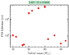 |
Fig. C.1. Variation of the puffed-up stripped star (PSS) lifetime with initial mass with a high semiconvection variant (αSC = 100) at LMC metallicity. |
We expect this effect to play a role predominantly at low metallicity (SMC and below) and in a certain mass range that is model-dependent but generally above 15 M⊙. This is evident in our results (Fig. C.1). For models above 20 M⊙, the PSS lifetime increases dramatically. A similar effect could be played by very efficient rotationally-induced chemical mixing (Georgy et al. 2014)
Appendix D: Additional figures
All Tables
All Figures
|
Fig. 1. Hertzsprung–Russel diagram of two representative binary models of 16 M⊙ at metallicities 0.0068 (LMC) and 0.0017(0.1 Z⊙) starting from main sequence (MS) till core carbon depletion. Dotted diagonal lines represent lines of constant radius. The evolution stages are marked and labelled in various colours. The red dot represents the end of the main sequence (MS), and the blue square and pink diamond represent the end of core He burning (CHeB) and core carbon burning (CCB), respectively. The blue region represents the mass transfer phase, and the orange region shows the puffed-up stripped star (PSS) phase. Letters A to I mark the important instances in the star’s evolution (see text). The grey track ( |
| In the text | |
|
Fig. 2. Evolution of various quantities of a 16 M⊙ model (at LMC metallicity) with star age, near the mass transfer phase leading up to the puffed-up stripped star (PSS) phase. Panel (a) shows the variation of envelope mass and mass loss rate of the donor. The mass loss is mainly due to the transfer of mass to the companion but also contains contribution from winds. Panel (b) shows the effective temperature (green) and donor radius (blue), and panel (c) shows the magnitude computed in the F450W optical filter of the HST WFPC2 camera. The blue triangle and the black star represent the position where the flux ratio (fstripped/fcompanion) drops below 1 and 0.5, respectively. Panel (d) represents various luminosities contributing to the total energy output: the orange line represents the surface luminosity (Lsurf), the blue and green lines represent the luminosity to hydrogen burning (LH) and helium burning (LHe) respectively. The luminosity in the red dashed line is the luminosity due to gravitational contraction/expansion (Lgrav). The grey-shaded region represents the mass transfer phase, and the regions with dark lines represent the puffed-up stripped star (PSS) phase. |
| In the text | |
|
Fig. 3. Variation of various timescales with initial mass at SMC metallicity. The blue line represents the thermal timescale, and the orange line represents the puffed-up stripped star (PSS) lifetime. As can be seen, the PSS lifetime is ∼10–100 times longer than the thermal timescale. It is closer to the Helium burning lifetime, represented by a green line. |
| In the text | |
|
Fig. 4. Variation of the relative contribution of shell burning and winds to the hydrogen envelope depletion rate during the PSS phase, as a function of the initial donor mass. The yellow parts represent the contribution of shell burning, and the green region represents the contribution of winds. Red and blue lines represent LMC and SMC composition, respectively. The shell burning contributes more to the mass depletion of the envelope than the winds. The lines are extrapolated (dotted) to see the extent to which shell burning dominates. In the case of LMC, it is ∼54 M⊙, and in the case of SMC, it is 63 M⊙. Above this limit, the winds start to dominate the mass depletion of the envelope. |
| In the text | |
|
Fig. 5. Evolution of 16 M⊙ star in LMC composition considering no winds (left) and no composition changes (right). The colours and labels are the same as that of Fig. 1. For 16 M⊙, the winds play a subdominant role in stripping the envelope, and completely switching them off only prolongs the PSS phase by ∼1.3 times. On the other hand, in the hypothetical scenario with no composition changes due to burning (in particular H shell burning), the PSS phase would be much longer, by ∼4.7 times, illustrating the key role of shell burning in determining the evolution through the PSS phase. The green dots appear so close in the right plot, showing that the contraction happens very slowly as compared to the default scenario. |
| In the text | |
|
Fig. 6. Hertzsprung–Russel Diagram showing evolutionary tracks of the primary star in a binary system with initial masses 5, 6.5, 8, 10, 12, 16. 16.9, 20, 22, 26, 30 and 40 M⊙ at LMC metallicity. The blue lines represent the mass transfer phase, and the orange lines represent the puffed-up stripped star (PSS) phase. Red dots represent the terminal age main sequence (TAMS), and the blue squares represent the end of core Helium burning. The green dots are placed at intervals of 20 000 years starting from RLOF. The clustering of these dots towards the left shows that the star spends a long time in this phase. |
| In the text | |
|
Fig. 7. Variation of puffed-up stripped star (PSS) lifetime (tPSS) with initial donor masses (left) and corresponding luminosity (right) at various metallicity (represented by various colours). Dashed lines represent fits for the corresponding data. The bold dashed line guides the eye to illustrate the steepness of the slopes. |
| In the text | |
|
Fig. 8. Variation of the remaining envelope mass Menv (top) and average rate of Menv depletion (bottom) in stripped stars, plotted as a function of the initial mass. The combination of those two factors affects the duration of the PSS phase. |
| In the text | |
|
Fig. 9. Estimates of the number of PS stars that can be found at different mass ranges (left) and different luminosity ranges(right) at SMC (upper) and LMC (middle) and solar (lower) metallicities. Values above the bars in the upper right panel show the percentage of puffed-up stripped stars relative to the number of all stars in that luminosity bin, most of which are MS, based on Schootemeijer et al. (2021). |
| In the text | |
|
Fig. 10. Duration of the puffed-up stripped star (PSS) stage when the flux of the PS star in the optical F450W filter is at least equal (dashed) or half (dotted) the flux of its companion, for two assumed companion luminosities (red and green, see text), compared to our default PSS stage criteria based on the HR diagram position (black, solid). These are calculated at SMC metallicity. |
| In the text | |
|
Fig. A.1. Evolutionary tracks of 16M⊙ models at LMC metallicity (with varied initial orbital periods (Pini)) on the HR diagrams. Various colours indicate the various values of Pini described in the legend. |
| In the text | |
|
Fig. A.2. Variation of initial orbital period Pini with puffed-up stripped star (PSS) lifetime of 16 and 30 M⊙ models at LMC metallicity. |
| In the text | |
|
Fig. A.3. Evolutionary tracks of 16M⊙ models at LMC metallicity (with varied initial mass ratio (qini)) on the HR diagram. Various colours indicate various mass ratios described in the legend. |
| In the text | |
|
Fig. A.4. Variation of initial mass ratio (qini) with puffed-up stripped star (PSS) lifetime of 16 and 30 M⊙ models at LMC metallicity. |
| In the text | |
|
Fig. B.1. Variation of the puffed-up stripped star (PSS) lifetime with wind strength for 16 and 30 M⊙ at LMC metallicity. |
| In the text | |
|
Fig. C.1. Variation of the puffed-up stripped star (PSS) lifetime with initial mass with a high semiconvection variant (αSC = 100) at LMC metallicity. |
| In the text | |
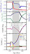 |
Fig. D.1. Same as Fig. 2, but for 3 M⊙ primary |
| In the text | |
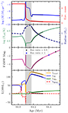 |
Fig. D.2. Same as Fig. 2, but for a 6.5 M⊙ primary |
| In the text | |
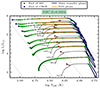 |
Fig. D.3. Same as Fig. 6, but for SMC metallicity |
| In the text | |
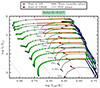 |
Fig. D.4. Same as Fig. 6, but for solar metallicity |
| In the text | |
Current usage metrics show cumulative count of Article Views (full-text article views including HTML views, PDF and ePub downloads, according to the available data) and Abstracts Views on Vision4Press platform.
Data correspond to usage on the plateform after 2015. The current usage metrics is available 48-96 hours after online publication and is updated daily on week days.
Initial download of the metrics may take a while.