| Issue |
A&A
Volume 687, July 2024
|
|
|---|---|---|
| Article Number | A257 | |
| Number of page(s) | 19 | |
| Section | Planets and planetary systems | |
| DOI | https://doi.org/10.1051/0004-6361/202349018 | |
| Published online | 23 July 2024 | |
PDS 70 unveiled by star-hopping: Total intensity, polarimetry, and millimeter imaging modeled in concert
1
European Southern Observatory,
Alonso de Córdova 3107, Vitacura Casilla
19001,
Santiago,
Chile
e-mail: This email address is being protected from spambots. You need JavaScript enabled to view it.
2
Université Côte d’Azur, Observatoire de la Côte d’Azur, CNRS,
Laboratoire Lagrange, Bd de l’Observatoire, CS 34229,
06304
Nice cedex 4,
France
3
Université Grenoble Alpes, CNRS, Institut de Planétologie et d’Astrophysique (IPAG),
38000
Grenoble,
France
4
School of Natural Sciences, University of Galway,
University Road,
H91 TK33
Galway,
Ireland
5
Indian Institute of Astrophysics,
India
6
University of Potsdam,
Germany
7
Instituto de Estudios Astrofísicos, Facultad de Ingeniería y Ciencias, Universidad Diego Portales,
Santiago,
Chile
8
Department of Astronomy, University of Florida,
Gainesville,
FL 32611,
USA
Received:
19
December
2023
Accepted:
11
April
2024
Abstract
Context. Most ground-based direct-imaging planet search campaigns use angular differential imaging that distorts the signal from extended sources, such as protoplanetary disks. In the case of the young system PDS 70, for which two planets were detected within the cavity of a protoplanetary disk, obtaining a reliable image of both planets and the disk is essential to understanding planet-disk interactions.
Aims. Our goals are to reveal the true intensity of the planets and disk without self-subtraction effects for the first time, search for new giant planets beyond separations of 0.1″, and to study the morphology of the disk shaped by two massive planets.
Methods. We present YJHK-band imaging, polarimetry, and spatially resolved spectroscopy of PDS 70 using near-simultaneous reference star differential imaging, also known as star-hopping. We created a radiative transfer model of the system to try to match the near-infrared imaging and polarimetric data within measurement errors. Sub-millimeter imaging data from ALMA were also modeled. Furthermore, we extracted the spectra of the planets and the disk and compared them
Results. With strong constraints, we find that the disk is quite flared, with a scale height of ∼15 at the outer edge of the disk at ∼90 au, similar to some disks in the literature. The gap inside ∼50 au is estimated to have ∼1 of the dust density of the outer disk. The northeast outer disk arc seen in previous observations is likely the outer lip of the flared disk. Abundance ratios of sub-micron, micron, and grains estimated by the modeling indicate a shallow grain-size index greater than −2.7, instead of the canonical –3.5. There is both vertical and radial segregation of grains. Planet c is well separated from the disk and has a spectrum similar to planet b, and it is clearly redder than the disk spectra. Planet c is possibly associated with the sudden flaring of the disk starting at ∼50 au. We found no new planets in the system. If we assume DUSTY models and an age of 5 Myr, this indicates no new planets more massive than 5 outside a 12 au separation.
Key words: protoplanetary disks / circumstellar matter / planetary systems / stars: individual: PDS 70 / stars: pre-main sequence / stars: variables: T Tauri, Herbig Ae/Be
© The Authors 2024
 Open Access article, published by EDP Sciences, under the terms of the Creative Commons Attribution License (https://creativecommons.org/licenses/by/4.0), which permits unrestricted use, distribution, and reproduction in any medium, provided the original work is properly cited.
This article is published in open access under the Subscribe to Open model. This email address is being protected from spambots. You need JavaScript enabled to view it. to support open access publication.
1 Introduction
Astronomers have detected thousands of mature planetary systems (ages > 1 Gyr) with exo-Neptunes, Jupiters (and some near exo-Earths), whose planetary properties have been analyzed to understand the end points of planet formation (Zhu & Dong (2021)). They have also detected hundreds of young systems (ages < 0.1 Gyr). These form an image of the embryonic phases of the planet-creation story. Recently, observers have started to discover systems going through the planetary birth process (Andrews (2020)). Since this phase is short (≲10 Myr), such bf cases are rare (Benisty et al. 2023), and PDS 70 is a prime example of such a system.
The PDS 70 proto-planetary system is in the midst of forming at least two giant planets (Keppler et al. 2018; Haffert et al. 2019) from a disk of gas and dust (Dong et al. 2012). This system represents an invaluable trove of clues to understanding the evolutionary steps of a disk during the planet-formation process (Bae et al. 2019). The age of the PDS 70 system is estimated to be around 5 Myr, placing it beyond typical disk lifetimes (see Müller et al. 2018, also Haffert et al. 2019; Skinner & Audard (2022) for discussion of the age of the system and the related estimates of planet mass). It is a K7 pre-main-sequence star with a mass of (0.82) solar masses (Riaud et al. 2006) and [Fe/H] = −0.11±0.01 dex (Swastik et al. 2021). The Gaia EDR3 motions of PDS 70 are consistent with it being a member of the Upper Centaurus Lupus star-forming region. The membership probability is as high as (98.7%), as determined using Banyan Σ (Gagné et al. 2018). The age of PDS 70 is significantly younger than the mean age of stars in the Upper Centaurus Lupus region (16 ± 2 Myr), but given that the instrinsic age spread is estimated to be ∼8 Myr, this is not surprising (Pecaut & Mamajek (2016)).
The system hosts two known planets, PDS 70 b and PDS 70 c, both of which are still in their formation stages (Benisty et al. 2021; Mesa et al. 2019). Their masses are estimated to be less than 10 MJ (Wang et al. 2021; Mesa et al. 2019). The planets are located at approximately 22 and 34 au from the central star (Müller et al. 2018). Atmospheric models applied to the planets suggest a temperature range of approximately 1000–1600 K and a surface gravity of log(g) ≤ 3.5 dex (Müller et al. 2018). Wang et al. 2021 found that requiring dynamically stable orbits results in a 95% upper limit on PDS 70 b's mass of 10 MJ. Their GRAVITY K-band spectra suggest dusty planetary atmospheres due to accreting dust. Mesa et al. 2019 have provided additional details, estimating PDS 70 c's mass to be less than 5 MJ, with an effective temperature of around 900 K and a surface gravity, log(g), between 3.0 and 3.5 dex. Using ALMA data, Benisty et al. 2021; Isella et al. 2019 have confirmed the presence of circumplanetary disks (CPDs) around both planets, with emission around PDS 70 c corresponding to a dust mass of approximately 0.031 M⊕ for 1μ-sized grains or 0.007 M⊕ for 1 mm-sized grains. However, the CPDs are not easy to detect in polarized light (van Holstein et al. 2021). Haffert et al. 2019 and Wagner et al. 2018 have both reported strong H-alpha emission from the planets, indicating ongoing accretion. Wagner et al. 2018 estimated the mass accretion rate for PDS 70 b to be 10-8MJyr-1 to 10-7MJyr-1, suggesting that the planet has acquired approximately 90% of its mass based on its current mass and accretion rate.
Both planets are thought to be in a 2:1 mean motion resonance, which has remained stable over millions of years (Bae et al. 2019; Haffert et al. 2019). PDS 70 b has an eccentricity of 0.17±0.06, while PDS 70 c has a near-circular orbit (Wang et al. 2021). PDS 70 b's orbit is co-planar to the disk, with a period of 118 yr (Müller et al. 2018).
The disk's gas and dust components have been extensively studied. ALMA observations with a spatial resolution of approximately 50 au have detected 16 transitions from 12 molecular species, including CO isotopologues, formaldehyde, small hydrocarbons, HCN, and HCO+ isotopologues (Facchini et al. 2021). ALMA observations have also revealed a radial dust gap at 0.42″±0.05 and peak densities at 0.75″ for the dust, 0.5″ for HCO+ J = 3–4, and 0.46″ for CO J = 3–2 (Facchini et al. 2021; Long et al. 2018). The gas disk exhibits a shallower gap depth compared to the dust. Also, the gas spreads wider than the dust disk (Facchini et al. 2021; Long et al. 2018). The disk is also characterized by strong X-ray and UV radiation absorption near the star, shielding the outer disk (Skinner & Audard (2022)). hboxCridland et al. 2023 used a thermo-chemical code called DALI (Bruderer et al. 2012; Bruderer (2013)) to model the radial profiles of 12CO, C18O, and C2H. They found a carbon-to-oxygen (C/O) ratio greater than one in the outer disk, corroborating Facchini et al. 2021's findings of a high C2H/12CO flux ratio. This suggests that the disk, and potentially the planets forming within it, could have a super-stellar C/O ratio in their atmospheres. Since the C/O ratio should change with distance from the star due to different condensation temperatures for the gases found, this could have implications for where the planets formed (hboxCridland et al. 2023).
In this work, we present near-infrared (NIR) observations of the system obtained with the SPHERE instrument at the Very Large Telescope (VLT). These include YJHK-band total intensity imaging and spectroscopy and H-band polarimetry. We used these data along with ALMA observations from Benisty et al. 2021 to create a consistent radiative transfer model of the disk. We then compared the astrometric and spectroscopic properties of the planets to the model disk properties in order to understand the interactions of the planets and the disk. The paper is organized as follows. In Sect. 2, we describe the observations and data reduction. Section 3 details the extraction of the planet photometry, astrometry, and spectra. We also extracted the disk spectra. We used the astrometry to find the most likely orbital solutions for the planets. Section 4 describes the radiative transfer modeling of the disk. In Sect. 5, we discuss the implications of the disk model and planet properties. In Sect. 6, we summarize our conclusions.
2 Observations and data reduction
The new observations presented in this paper were carried out using the SPHERE instrument (Beuzit et al. 2019), installed at the Nasmyth Focus of unit telescope 3 (UT3) at the VLT. SPHERE is a state-of-the-art high-contrast imager, polarimeter and spectrograph, designed to find and characterize exoplanets. It can deliver H-band Strehl ratios for bright stars (R<9) of up to 90%, and continue to provide AO corrections for stars as faint as R = 14. SPHERE also provides coronagraphs for starlight suppression, including apodized Lyot coronagraphs (Soummer (2005)). It is comprised of three subsystems: the infrared dual-band imager and spectrograph (IRDIS; Dohlen et al. 2008), an integral field spectrograph (IFS; Claudi et al. 2008) and the Zurich imaging polarimeter (ZIMPOL; Schmid et al. 2018).
We observed PDS 70 in IRDIFS (IRDIS+IFS) (Vigan et al. 2010; Zurlo et al. 2014) and IRDIS-DPI modes (de Boer et al. 2020; van Holstein et al. 2020; van Holstein et al. 2017) on six nights between July 2021 and February 2022. Except for the July 2021 and the February 2022 observations, all were poor weather or partial datasets aborted because of worsening conditions. However, since we observed using star-hopping RDI (Wahhaj et al. 2021), good reference point spread functions (PSF) could be subtracted to obtain useful data even for the aborted observations. This is because signal self-subtraction from insufficient sky rotation is not a problem, as it would be in Angular Differential Imaging (ADI). The observing parameters of the SPHERE observations are presented in Table 1. In summary, we observed PDS 70 with IRDIS H-band obtaining Stokes Q and U, and total intensity images. We also obtained simultaneous IRDIS Ks-band imaging and IFS R = 40 spectroscopy over the YJH-band region. We used the N_ALC_YJH_S coronagraph, which has a mask radius of 93 mas and was designed for the Y±K band range, with an overall transmission of 58% (Beuzit et al. 2019).
2.1 Total intensity
IRDIS dual-band images in the Ks-band and IFS R ∼30±50 spectra (in the Y±H range) are obtained simultaneously. The IRDIFS data were obtained in 1.5 h observing blocks (OBs), interleaving observations of PSF reference star with science observations. For the reference star, UCAC2 14412811 (R = 11.7, H = 8.9 vs. R = 11.7, H = 8.8 for PDS 70), a 6 min sequence was obtained after every 10 min of science, with only 1 min taken to hop back and forth between the two targets. This star is separated 0.64∘ from PDS70, and thus ideal as a PSF for reference differential imaging (RDI). This mode of RDI observations is called star-hopping (Wahhaj et al. 2021).
The star-hopping data are reduced according to the standard pipeline described in Wahhaj et al. 2021, with modifications to prioritize detecting extended emission over point sources. The details of the pipeline will be described in Swastik et al. 2024. In summary, the area used to match the science and reference PSF is chosen to be partly inside the coronagraph (separations 0.04″ to 0.08″), and the region which includes the speckle ring right outside the AO control radius. Since these are typically regions where circumstellar emission does not dominate, the disk emission is preserved beyond separations of 0.1″. For creating the best reference PSFs to subtract from each science image, we select the best 16 reference images based on the standard deviations of science±reference difference pairs. Then, the LOCI algorithm (Lafrenière et al. 2007) is used to create the best linear combination of reference images, minimizing the standard deviation in the difference images in the regions used for matching. The final reduced images are shown in Fig. 1.
Observational setup for PDS 70 imaging datasets.
2.2 Polarimetry
We used the IRDAP pipeline (van Holstein et al. 2020) to reduce the H-band Dual-beam Polarimetric Imaging (DPI) mode data. IRDAP corrects for the instrumental polarization and polarization crosstalk, thereby attaining a polarimetric accuracy of <0.1%. IRDAP subtracts the stellar polarization signal. The reduced images are shown in Fig. 1. The Qϕ and Uϕ images are shown in Appendix A for reference only, as we did not use them in our disk modeling efforts. We remind the reader of a few key points on polarimetry and particular conventions used by the IRDAP pipeline, but for further details please review de Boer et al. 2020. We measure polarization with respect to chosen axes: the north-south axis on sky denoted Q+, and the east-west axis denoted Q−. We chose axes (as opposed to directions) since the E-field changes direction from positive to negative as a light wave propagates. The Stokes Q image is the difference in the time-averaged electric field intensity between the Q+ and Q− axes. The Stokes Q, U, and V images, which are practical to measure, represent intensity differences which together with the unpolarized light fraction constitute the total intensity of the observed light (see de Boer et al. 2020). The Radmc3D code, which we will use to perform radiative transfer modeling of the PDS 70 disk, generates Stokes Q images with Q+ aligned along the horizontal axis, and north pointing right, east pointing up. Thus, to match the IRDAP orientation, we rotated the Radmc3D images anticlockwise by 90∘ so that Q+ is vertical, north is up, and east is left.
3 Planet search combining true-intensity imaging and polarimetry
Angular Differential imaging (ADI) typically subtracts a significant fraction of circumstellar disk flux in a non-uniform fashion, as the science images themselves are used for PSF subtraction (Marois et al. 2006; Milli et al. 2012). This is facilitated by decoupling the pupil (thus PSF) and sky rotation, by controlling the telescope de-rotator. Thanks to star-hopping RDI, we have obtained a self-subtraction-free high-quality total intensity image of the disk in H-band. Such imaging obtained simultaneously with polarimetry is a first for PDS70. Other transition disk systems have recently been observed in such a mode (Renbreak et al. 2023).
Our novel observational method allowed us to search for planets in a new way. Planet atmospheres should scatter light with low polarization fractions, while the disks are expected to scatter with much higher polarization (Stolker et al. 2017). Thus, the ratio of the linearly polarized intensity  and the total intensity, could reveal planets as dips or negative Gaussians superposed on a bright polarization fraction map. We used the inverse map so that planets would show up as bright spots. Such a map should only be trusted in the regions where the denominator has a high S/N, that is, not close to 0. Thus, when the S/N falls <5, the polarized intensities are set to the constant value corresponding to an S/N of 5. The inverse map,
  , which should show planets as bright spots, is shown in Fig. 2. Planet b was clearly detected but not planet c. The method failed for planet c because
  has a very low S/N at that location and thus provides a flat divisor, so there is no signal boost for planet c. Another problem is that planet b and the front part of the disk appear comparably bright in the map, indicating that both have low-polarized fractions. Thus, we conclude that this method would only be useful in the case of a low-polarization planet superposed on a high-polarization disk detected at a high S/N.
3.1 Improved planet extraction in disk systems
Detecting planets is more difficult when imaging bright disk systems. The disk emission is so strong in the PDS 70 NIR images that it interferes with the PSF subtraction. Thus, we attempt to subtract a smoothed version of the disk, along with the subtraction of the reference star's PSFs. This time LOCI is used to match the PSFs over the 0.1″±1.5″ annulus centered on the star, instead of trying to avoid the disk regions as in the first-round reduction (see Sect. 2). The smoothed disk image is made by median smoothing the disk image we obtained in the first-round reduction, over a box size of 12 pixels. The median smoothing removes most of the point sources and sharp features in the disk. Thus removing the smoothed disk from the data should not remove candidate companions. This works better than unsharp-masking the images prior to reduction, because unsharp-masking leaves strong artifacts from the disk in the images. In Fig. 3, we see the first unambiguous detection of planet c in the NIR. We measure of the location of the planet using the IDL bscentrd routine, a very robust routine centroiding routine we tested extensively in Wahhaj et al. 2013. We estimate the S/N of planets b and c to be 11.5 and 5.5, respectively. It is also clear that there are no other planets as bright as planet c detected in the image, beyond a separation of 0.1″ from the star (beyond the coronagraph). It is possible that the disk is hiding a brighter planet or CPD than planet c. Planet c clearly lies in the gap, just inside the inner edge of the disk. This reduction demonstrates the effectiveness of subtracting a smoothed disk along with the reference star PSFs, in isolating and detecting point sources. Planet c was hardly noticeable in the reduced image of the disk presented earlier (see Fig. 1). The FWHM of both planet detections are 59 mas (∼7 au) very close to the Ks-band diffraction limit, indicating that any CPDs have compact emissions originating from close to the planets.
The Ks-band image reveals the PDS 70 circumstellar environment beyond 0.1″ (the coronagraph radius). To find the detection limits as a function of separation, we calculate a simple 5σ contrast curve as 5 σ(r)(estimated stellar peak), where σ(r) is the robust standard deviation as a function of separation. The stellar peak is estimated from the background object to the north (Riaud et al. 2006); Hashimoto et al. 2012), which had PA = 14.1∘, separation = 2.62″, ΔK = 4.58 mag in our non-coronagraphic short-exposure images, which detected both stars without saturation. The background object is also well-detected yet unsaturated in all our science images. We take the robust σ(r) to reduce the disk's effect, which is already attenuated by removing the smoothed disk, as mentioned above. However, we indicate in Fig. 5 the detection-limit on the brightest part of the disk, 3.4 MJ. Thus planets of that mass could be obscured where disk detection is strong.
Given the complexity introduced by the disk residuals and the two planets, in the smooth-disk subtracted reduction, improved contrast estimation by recovery of simulated planets is difficult. Nevertheless, we injected simulated planets in the more cleared regions of the system, into the basic reduced images, at twice the fluxes of the detection limits. We started the injections started at a PA of 225∘ and 0.1″ separation, incrementing the polar coordinates by 0.1″ and 90∘ for each subsequent planet. A first round reduction of this dataset was achieved exactly as before while trying to preserve the disk. Again, a smoothed version of the reduced image, this time with the simulated planets and the disk, is supplied as a reference image for a second round of LOCI reduction. This is basically a repeat of the smooth disk-subtracted reduction. The resulting image is shown in Fig. 4. Since there are few clear regions in the disk, the flux uncertainty as a function of separation is estimated from this single reduction only. The detections of the simulated planets passed criteria based on S/N and shape discussed in Wahhaj et al. 2013. We take twice the difference between the actual flux of a simulated planet (in a 2-pixel radius aperture) and the recovered flux as the uncertainty, although this would normally be considered the systematic error and not the random error. Thus, we estimate the uncertainties as 0.26 mag at 0.1″ and 0.12 mag at larger separations. The mass estimates resulting from this photometry, assuming an age of 5±1 Myr (Müller et al. 2018) and hot start models (Baraffe et al. 2003) are presented in Table 2.
We reach an unprecedented detection limit of 5 MJ at 0.1″ separation. Compared to past observations, in our novel detection space of ∼11 to 22 au, we find no new planets. This improved sensitivity to planets is due to better stellar PSF subtraction, thanks to star-hopping RDI and the smoothed disk subtraction, as opposed to what is achievable with just ADI, especially in the presence of disk signals. The deepest contrast is reached at a separation of ∼90 au, where the detection limit is 2.3 MJ.
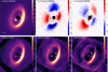 |
Fig. 1 SPHERE Observations of PDS 70. Top row, left to right: IRDIS Ks-band, Stokes Q/H-band, and Stokes U/H-band images. Bottom row: H-, J-, and Y-band IFS observations, median combined over the typical band widths. North is up, east is left, and the black circle in the center is a mask over the coronagraphic region. |
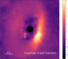 |
Fig. 2 Inverted H-band polarized fraction map given by |

 |
Fig. 3 IRDIS Ks-band reduction to bring out the planets by trying to remove the disk. A smoothed version of the disk reduction (median smoothed over 12 pixel boxes) along with the PSFs of the reference star was supplied to the LOCI algorithm in order to subtract both the disk and star. |
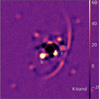 |
Fig. 4 IRDIS Ks reduction to recover simulated planets and detection limits as shown in Fig. 5. The disk has been subtracted as described in the text. The real planets b and c are labeled. |
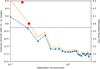 |
Fig. 5 IRDIS Ks-band detection contrast limit for S/N >5 (shown with the blue curve). It was made from the simulated planet recovery, as explained in the main text. The orange line shows the limits corrected for small sample statistics according to Mawet et al. 2014. The mass detection limits are estimated from the DUSTY models, assuming an age of 5 Myr for PDS 70. The dashed line represents the detection limit at the brightest part of the disk. |
Planet properties.
3.2 Spectra extraction
We can extract the planet spectra from the 39 Y±H-band IFS channels, at the locations of the planet detections in the Ks-band image. We use an aperture of radius 3 spaxels (7.46×7.46 mas) to extract flux per IFS channel at five spots: two on the planets, and three on selected bright parts of the disk (see Fig. 6). These IFS channel fluxes are divided by the stars' channel fluxes, obtained from the non-coronagraphic FLUX observations. To obtain the final spectra in Fig. 6, we multiply these channel flux ratios by the stars' actual spectra (obtained with the XSHOOTER instrument by Campbell-White et al. 2023).
As in the IRDIS reduction, we estimate the flux uncertainty in each spectral bin to be 0.25 mag, which indicates that the uncertainly in the first order slope of the spectra is ∼4% (0.25 mag  .) Thus, it seems that the planet b and c spectra are quite similar to each other and are clearly redder than the disk spectra over the YJH-bands. Particularly, the planet spectra peak around 1.27 μ and between 1.5 and 1.67 μ, while they are clearly suppressed between 0.9 and 1.15 μ , relative to the disk. The J and H-band features are likely due to methane absorption (see Pluto's spectra in Grundy et al. 2013). The disk spectra along different lines of sight are also very similar. One may argue that the aperture flux obtained at planet c location has disk contributions to it, and also that our planet b spectrum does not have proper background subtraction. But the fact that we can differentiate between planet and disk spectra despite these potential systematic biases indicates that the differences in the spectra are likely real.
The main reason for the difference between disk and planet spectra is that the planet atmospheres are around 1100 K (Wang et al. 2021), whereas the disk is much colder. The evidence for the CPD comes from the Hα accretion signature (Haffert et al. 2019) and the ALMA 855 μ detection (Isella et al. 2019). In contrast, the JHK-band spectra seem to originate from the planetary atmospheres and not from the CPDs. The spectra also suggest a good way to distinguish between planets and disk material.
3.3 Orbit fitting
We use the astrometry collated by Benisty et al. 2021, along with those from our epochs (see Table 3) to find constraints on the orbits of planets b and c. Planet c's orbit is less well known than planet b's, as it has been detected in fewer epochs and with a smaller S/N. We use the orbitize! Python package written by Blunt et al. 2017 to find the most likely orbital solutions.
We use the package's MCMC method, sampling 1 000 000 orbits. The results are shown in Figs. 7, E.1 and E.2. For both planets, the eccentricities are likely >0.2 and <0.7, favoring significantly eccentric orbits. Planet b's orbital constraints are semi-major-axis (SMA) =  au, eccentricity =
  and inclination =
  (subtracting from 180°), consistent with that of the disk.
Planet c's orbital constraints are semi-major-axis (SMA) =  au, eccentricity =
  and inclination =
  (subtracting from 180∘), again consistent with that of the disk.
We note that 2:1 mean-motion resonance (MMR) orbits are allowed by our constraints, for example, if we assume SMA of 14 and 22.2 au for planets b and c respectively. These SMA lie within a 75% confidence interval in our constraints. Thus, reasonably stable orbits should allowed by our constraints. An SMA of 22.2 au corresponds to a maximum separation of 32.6 au (=SMA![Mathematical equation: $[1+e]$](/articles/aa/full_html/2024/07/aa49018-23/aa49018-23-eq12.png) ) from the star, which would mean that planet c orbits far away from the gap edge at 49.7 au. Since we can now easily extract planet c's astrometry using our new RDI with disk subtraction technique (see Sect. 2), better orbital fits should be forthcoming in the near future.
) from the star, which would mean that planet c orbits far away from the gap edge at 49.7 au. Since we can now easily extract planet c's astrometry using our new RDI with disk subtraction technique (see Sect. 2), better orbital fits should be forthcoming in the near future.
Our constraints are somewhat more relaxed than those found by Wang et al. 2021 as we do not impose any additional constraints on the orbits. Quite justifiably, Wang et al. 2021 imposed requirements that the orbits should be co-planar, stable for 8 Myrs, and not have peri-astrons that exchange order over their lifetimes. We also found the orbital constraints using only the astrometry from Wang et al. 2021, and these were quite similar to the ones presented here. Thus, we note that we found higher eccentricities for both orbits not because of our new astrometric points but because we did not impose the stability conditions of Wang et al. 2021. Given the significant eccentricities, the planetary orbits may become unstable given another 5 Myr.
New astrometry for planets b and c.
4 Radiative transfer disk modeling
In this section, we model the three main datasets: total intensity K-band imaging, polarimetric H-band imaging, both of which are from the SPHERE instrument, and 870 µm imaging from ALMA (Benisty et al. 2021). We produce models of a flared protoplanetary disk of gas and dust, using the radiative transfer code Radmc3D (Dullemond & Dominik (2004)). Given that each model takes about 1 min to produce, and given the high information content of our datasets, we do not attempt to converge on a true best fit model. Rather, we attempt to find a model that is broadly consistent with the data given our computational constraints. We also study the constraints on our parameters by exploring the χ2 space around the best-fit model. Thus we find a range of models that are broadly consistent with the data, but do not claim that these are formal constraints.
4.1 Search for a convergent model
Given that we had to obtain a good model in a reasonable amount of time, the choice of the metric to minimize was important. Ordinarily, we would choose the total χ2 metric, adding the χ2 for the three images and three flux measurements. But using the total χ2 metric would force search algorithms to prioritize minimizing the χ2 for the highest resolution image, since it contributes the most to the total χ2. If the search has not yet converged on the actual minimum, the current best model may poorly fit the smaller data components, such as the band photometry and low-resolution images. Instead, we use the average reduced χ2 of all the images and photometry, so that they have equal weight in the combined metric. For more details, see Appendix B. We warn that our model searches are only locally convergent, but may be missing the global minimum. However, since we repeated the searches many times, exploring reasonable guesses at improved initial parameter values, better solutions would be very difficult without considerably more computing power.
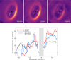 |
Fig. 6 IFS observations. Top: YJH-band images made from collapsing the IFS spectra and the locations from which the planet and disk spectra were extracted. Bottom: IFS Spectra of the b and c planets along with spectra of this dust ring at three locations. The planet spectra are similar to each other, and clearly different from the disk spectra. The region contaminated by telluric absorptions around 1.4 μ is grayed out. |
 |
Fig. 7 Orbit fitting using astrometry from this work and earlier studies for planet b (left) and c (right). The best 500 orbits from 1 000 000 orbits fitted by the orbitize! package (Blunt et al. 2017) are shown along with predictions of separation and PA for the near future. |
4.2 Model parameters
Our first order model is chosen to be a flared disk of gas and dust extending from ∼0.1 au to 100 au, with a gap inside this disk (see schematic in Fig. 8). This model is inspired by the findings of previous studies on PDS 70 (Keppler et al. 2018; Portilla-Revelo et al. 2022; Benisty et al. 2021), and our own Ks-band image. On a cursory examination of our data, we note that the ALMA image shows a flat disk, while the SPHERE NIR images show a flared-disk. This indicates a vertical settling of large grains (millimeter sized). Thus, we used multiple populations of grains that are allowed to spatially segregate. Each grain population is said to constitute a disk zone. Initially, we attempt to fit the data with a two-zone model and later complexify it with a third zone. In the NIR images, we also notice that the disk is much brighter in the southwest (SW) direction, which suggests significant forward scattering. This portends the existence of micron-sized grains. However, since the northeast (NE) side is also well-detected, there must be sufficient back-scattering grains, especially in the polarimetric images. According to our modeling experience, this indicates the presence of sub-micron grains.
Our radmc3D models were made at low-resolution for reasons of computational speed, as we describe in Appendix B. However, once we had converged on a best-fit model, we re-ran the models at a higher resolution to check if there were vast changes in fit quality. Since this was not the case, we consider the resolution of our models to be adequate. We note here that the model images were convolved with Gaussians of width equivalent to the PSFs of the observations.
Each disk zone is described by the following: 1) a grain size, a; 2) an inner radius Rin; 3) an outer radius Rout; 4) a scale height H  , where r is the stellocentric distance; 5) a dust density power law r-γ 6) a disk mass M; 7) a position angle PA; and 8) an inclination angle i with respect to the plane of the sky. Most of these parameters are common to all disk zones. However, some zone parameters were allowed to be independent, specifically grain sizes, zone disk masses, scale height, and γ. We note here that Rin and Rout are the same for all the zones. Also, between the star and Rin there is a gap which has only a fraction (e.g., 1%) of the exterior dust density. We call this fraction gap clearing. The dust grains were modeled as amorphous olivine with 50% Mg and 50% Fe, or pyroxene grains with 70% Mg and 30% Fe, both of which are used often in the literature (Jaeger et al. 1994; Dorschner et al. 1995). We used the Powell algorithm (Powell (1964)) to improve the fit, after several iterations of parameter estimation by eye, which proved to be much more efficient. The Powell algorithm is known to be robust and efficient for minimization over many variables, when the gradient of the optimization metric is not known a priori. To calculate χ2, we follow the method of Wahhaj et al. 2005, where the χ2 are normalized according to the number of significant resolution elements they represent (see details in Appendix B).
4.3 Best two-zone model
The best-fit two-zone model, which has 14 free parameters, was compared to the observed images and residuals after differencing in Fig. 9. The model parameters are shown in Table B.1. Qualitatively, all the salient features in the data seem to be present in the two-zone model: a deep gap 50 au in the inner disk, the polarimetric model image shows an optically thick flared disk, the sub-millimeter model shows a flat disk, the NIR total intensity model shows an outer arc NW of the disk, and strong forward-scattering, while the polarimetric model images also show some back-scattering. The flux comparisons yield reduced χ2 s close to one, indicating good matches. However, several short-comings of the model are already evident to the eye, as we discuss below. Moreover, the image model comparisons yield reduced χ2 values that indicate poor fits (see Table B.2), despite the fact that most of the disk flux has been subtracted. This is not surprising since the observations are of such high signal-to-noise and resolution that they warrant highly complex models with ∼100 parameters, given that our observations represent 2000 data points (>1000 resolution elements with a high S/N; see Table B.2 and Appendix B).
A clear deficiency of the two-zone polarimetric model is insufficient disk emission from the northern and southern parts of the disk (which indicates deficit of light with E-field oscillating east-west). From our modeling experience, this deficit seems unavoidable for grain sizes ∼0.5±1μ, where the grains have a non-trivial polarimetric phase function. Grains above this size are too forward-scattering to satisfy the polarimetric image, while grains below this size do not forward-scatter enough to satisfy the total intensity NIR image. The disk flaring required for the micron-sized zone also seems unrealistically high (13% at Rin and 150% at Rout). The 870 μm model flux is double the data flux, suggesting that we need grains with a higher albedo to scatter more light in the NIR and produce less thermal emission in the sub-millimeter. Pyroxene grains may be used to compensate for this limitation. We then experimented with adding a third disk zone with sub-micron grains and allowing pyroxene grains where helpful. We describe this in the next section.
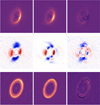 |
Fig. 9 Comparison of Radmc3D preliminary two-zone model images with data. The figure shows poor fits to the polarimetry data. The left, middle, and right columns represent the data, model, and residual, respectively. The top, middle, and bottom rows are the Ks-band total intensity image, H-band Stokes Q image, and ALMA 870 μ image, respectively. The data and model images are of the same resolution. |
4.4 Best three-zone model
For the three-zone model, we allowed the search algorithm to pick between olivine or pyroxene grains for each zone. Also, Zone1 and Zone2 are forced to have the same properties except for dust mass and grain size. Zone3 was allowed to have a different dust mass, grain size, β, H, and γ. In summary, we had 17 free parameters compared to the 14 of the two-zone model. The model parameters are shown in Table 4. The best-fit three-zone model is compared to the observed images in Fig. 10. The flux in the sub-millimeter is now very well-matched by the model. The disk flaring for the micron and submicron zones also seem much more realistic (2.6% at Rin and 15% at Rout). The emission in the northern and southern parts of the disk are now much better matched by the polarimetric models, which is indicated by the improved χR2 of 7 (see Table 5. Compare to 15 for the two-zone model in Table B.2). Since the total χ2 decreases by ∼3600 using only three more parameters, the three-zone model is clearly preferred by the data.
However, the residuals in the difference images suggest that model improvements could be made by adding more parameters. The residuals show emission from the back side of the disk rim beyond 50 au, in the Ks-band total intensity image. This could be compensated for by submicron grains with a slightly different composition so that they maintain good total flux and polarimetric matches. This is not possible with our grain models. The polarimetric residuals in the H-band show too little forward scattering (see the east and south sides of the disk). Again, this could be addressed by micron-sized grains, which don't invoke too much forward scattering in the Ks-band image. We find that individual fits to either the Ks-band are much better than a combined fit, and this is mainly because a good balance between forward and backward scattering, or between submicron and microns grains is hard to achieve. The ALMA image model is clearly inadequate, as it is unable to reproduce the sharp edge to the bright ring at 0.5″. The smooth brighter edge in the model is created by a modest flaring (1.3% at Rin and 7.5% at Rout). The observed sharp ring could be made by an additional dust component, shaped by a different phenomenon. The residuals also give evidence for asymmetries, which could be accounted for by disk ellipticity or local density perturbations. In summary, the models show that the major features of the disk emission can be described rather simply.
In Fig. 11, we compare the three-zone model images with Y, J, and H-band IFS observations, median combined over the typical band widths. For these, the models were not fitted because of computational limits. However, the morphology and brightness of the model images are very similar to the data in all bands, suggesting reasonable matches. The Y-band match is poorest, showing “patchy” residuals, seemingly due to PSF halo mismatch at large scales. Notably, the dominance and degree of forward-scattering over backward scattering, the curvature at the outer part of the disk, and the depth and clarity of the disk gap are satisfactorily reproduced.
4.5 Constraints on model parameters
Calculating uncertainties is a challenge because we cannot fully rely on our results from Monte-Carlo style Bayesian estimation (using the Python emcee package). This is because we were only able to run ∼38 000 samples (see Appendix D) given that each model takes 1 min to create. This is just an unavoidable computing power limit, given the very high resolution of our data. In our estimate, the Bayesian uncertainties are too small. Thus, we attempted to estimate the uncertainty of our best-fit in the local minimum. To achieve this, we first computed the χ2 for each parameter by varying it along a linear grid, flanking the optimal fit value. During this process, we allowed the other 16 parameters to adjust accordingly, to identify a set of best-fit solutions. The uncertainty for each parameter was then determined based on the range within which the change in χ2 remained below 1% of the minimum value. This 1% threshold was chosen because the uncertainty in our χ2 estimates themselves are around 0.5%. Although we cannot claim that we have found a true best-fit model, or robust uncertainties, we do show whether these constraints from the local minimum are weak or strong.
The uncertainties of the three-zone model are shown in Table 4. The majority of the parameters are extremely tightly constrained at the local minimum, implying that we get very poor fits for slight variations (1±2%). These strong constraints are possible because of the high S/N and resolution of our images. Some highly constrained parameters are Rin, Rout, PA, i, and the mass in Zone2 (the micron-sized grain disk). The strong Zone2 mass-constraint comes from the delicate forward and back-scattering balance of the NIR images. We also note relatively strong constraints (∼5%) on the scale height and flaring parameter β for Zone1 and Zone2, which just means the flaring in the disk is real and well-detected. Flaring in Zone3 is only needed to make the outer edge of the disk brighter, but it is also constrained to be small. The density power-law index of Zone1 and Zone2 is strongly constrained to have a minimum steepness, and is found to have the typical range for flared disks. There is a strong upper limit of the gap clearing fraction ( ), indicating the gap is indeed largely cleared of dust. The lower limit, although softer, also indicates that some dust is needed. Soft constraints on the Zone1 and Zone3 masses and the Zone3 grain size are likely due to optical thickness requirements being soft. Once a certain optical thickness is reached, the images do no change much. On the other hand, the disk must be optically thick in the NIR to mask its far side and to appear flared. Likewise, the Zone3 grains, which make a flat disk, must not influence the NIR images, and therefore must be sufficiently large (and cold). But given their large size, and low total surface area, we need a high total mass to match the intensity of the ALMA image.
Three-zone model best-fit parameters.
Goodness-of-fit statistics for the three-zone disk model.
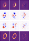 |
Fig. 10 Comparison of Radmc3D three-zone model images with data. The left, middle, and right columns represent the data, model, and residual respectively. The rows from top to bottom are the Ks-band total intensity image, H-band Stokes Q image, Stokes U image, and ALMA 870 μm image, respectively. |
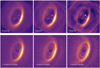 |
Fig. 11 Comparison of Radmc3D three-zone model images with Y-, J- and H-band IFS observations, median combined over the typical band widths. For these, the models were not fitted because of computational limits. Simulated noise has been added to the data, but no planets were simulated. The data and model are morphological very similar. |
5 Discussion
5.1 Disk model
We have found a model with a reasonably good match to the dust disk around PDS 70, which we demonstrate by calculating the χ2 from our highest S/N images. The most likely morphology is that of a highly flared disk with a deep gap within ∼50 au of the star. Moreover, the disk flaring is clearly detected in the H-band Stokes Q and U images. The NW outer disk arc seen in JHK observations is also naturally produced by the flared disk model (see van Holstein et al. 2021 and Juillard et al. 2022 for other possibilities). Although we could not present a model that is completely consistent with the data in terms of a χ2 comparison, the nature of the residuals show that these are minor deficits of the model, and not fundamental limitations in our understanding of the physics. The most likely model limitations are that we 1) varied the grain-size over a very coarse grid – 20% per step, 2) used a single grain size for each disk zone, not a size distribution, 3) did not try varying the ellipticity of the disk, and 4) used a monotonic dust density, except for the inner gap. In summary, although the search for a completely consistent fit is warranted, as this will help refine our description of the dust physics, there seems to be nothing mysterious about the model inadequacies. Thus the disk is flared in the NIR, flat in the sub-millimeter, and sub-micron to millimeter dust grains all occupy the same radial extent (∼50 to 90 au).
In the paper, we did not model the inner disk which was detected in Keppler et al. 2018, and likely appears in our images as small features to the top-left and bottom-right of the coronagraph. These features are quite compact and irregular, and so would make the modeling complicated. We thus leave this effort to a later analysis.
We can compare the number of grains for each size to check whether their ratios agree with the grain size distribution expected from a collisional cascade  , with
  (Dohnanyi (1969)) (see Appendix F). From the dust mass and grain size estimates of the three-zone model (see Table 4), we find that the 10.9 μm grains are over-abundant by factor of ∼2 compared to the 0.1 μm grains, while the 300 μm grains are over-abundant by a factor of ∼1000. To reconcile the number ratios for Zone1 and Zone3, we need to set ζ=−2.67. The sub-micron and micron grain numbers are both constrained by the NIR images. The total intensity images strongly constrain the micron-sized grains, demanding strong forward scattering and adequate optical thickness to give the disk a 3D appearance. The polarimetric images likewise demand both substantial forward and back-scattering. Furthermore, both grains populate the surface layers of the disk, thus indicate something about the true surface grain size distribution. These independent constraints make our ζ=−2.67 estimate an important measurement of the power law for a proto-planetary disk, enabled by self-subtraction-free imaging with star-hopping.
Taking the ζ=−3.5 power law as a reference, smaller grains are under-abundant, which suggests that their loss is efficient. Our shallower power law may be typical of proto-planetary disks, as opposed to debris disks or the ISM (Dohnanyi (1969); Draine (2006)). Although, sub-millimeter studies have yielded ζ ∼ −3.5 (Guidi et al. 2022), comparing NIR and sub-millimeter image may tell a different story. Probable causes for the relative lack of small grains could be 1) small grain leakage into the disk gap (Bae et al. 2019), 2) substantial grain-growth of sub-mm grains. Efficient grain growth in the disk mid-plane where the sub-mm grains settle could explain why the micron to sub-mm distribution is even shallower (see Fig. F.1).
5.2 Planets
We have found that planet c's spectrum is very similar to planet b's, while both spectra are much redder than that of the disk. This suggests that we are detecting the atmosphere, rather than a CPD for both planets. The CPDs, which are expected to be much colder (<500 K, see Wang et al. 2021) than the planet atmospheres, should have spectra more similar to the cold circumstellar disk's. As found by Wang et al. (2021), the evidence for the CPD comes from the emission at longer wavelengths (M-band and 855 μ detections). In the JHK-bands, planet c is not majorly shrouded or contaminated by the main disk's dust. Thus planet c is likely inside the gap as indicated by our orbital solution. It may seem that this fact should aid us in detecting planet c in a polarized fraction map, but we showed this was not the case. This is primarily because the polarimetric image needs to be much higher S/N for this technique to work.
To understand the planets' interaction with the gas and dust disk we look to the dynamical simulations by Bae et al. 2019. They studied the mass accretion of the planet and their orbital evolution in a disk of gas and dust, tracking the locations of different particle sizes. Many of our findings can be explained by their dynamical model. They find that the planets will quickly settle into a 2:1 MMR in ∼0.1 Myrs, and can then remain stable for at least 2 Myr. A 2:1 mean-motion resonance is consistent with our results, for example SMAb = 14 and SMAc = 22.2 au results in a 1:2 period ratio. These correspond to maximum separations from the star of 20.6 and 32.6 au (=SMA[1 + e]), respectively. In both our models, we find that planet c is clearly in the dust gap, and the apparent superposition with the disk is only a result of the inclination of the system. The sub-millimeter grains of the Bae et al. 2019 simulations are confined near the gas pressure maximum, in a particularly narrow radial range when planet c has a mass of 2.5 MJ which is closest to our estimate of 3.8±0.4 MJ. The location of this sub-millimeter ring is ∼75 au in the ALMA image, 63 au in their simulation, but is dependent on the planet masses and initial semi-major axes (SMA = 20 au and 35 au for planets b and c in their work). Presumably, an agreement could be found with the constraints in this work, if our SMA estimates were used. The smaller grains take a much more monotonic distribution than the sub-millimeter grains as we found in our best models. The dust density in their disk gap is also ∼1% of that of the outer disk, while the small grains are leaking into the gap.
In any case, we must ask why the disk flares sharply starting at ∼50 au, when the gas is spread vastly wider than the dust. The assumption is that the planets can keep the dust (especially the large grains) out of the gap, but not the gas. Both the Bae et al. (2019) simulations and the observations of Long et al. 2018 and Facchini et al. 2021 show that the gas density also drops significantly inside the gap. This should also decrease the disk scale height. Another way planet c could do this is by producing extra gas turbulence near its orbit, especially if its orbit is eccentric. A wider gap is cleared when the planets orbits have some eccentricity. However the eccentricity is only expected when the mass accretion onto the planets is ∼to 7 ×10⁻⁷ MJ yr−1, which is 10 times greater than the observed accretion rates (Wagner et al. 2018; Haffert et al. 2019). In summary, the observed morphology of the dust disk can be explained by the growth and orbital evolution of the planets.
6 Conclusions
In this work, we have presented YJHK±band imaging and spatially resolved spectroscopy along with H-band polarimetry of the PDS 70 system, which is characterized by multiple planets and a young disk. Our observations have unveiled the true intensity of both the planets and the disk without self-subtraction artifacts that are typical of ADI observations. This was achieved through the use of near-simultaneous reference star differential imaging, a technique also known as star-hopping. Our primary objectives were twofold. Firstly, we wanted to explore the presence of new giant planets located beyond separations of 0.1″, and secondly, we wanted to closely examine the disk's morphology in order to gain insights into its interactions with the orbiting planets. We used radiative transfer modeling, namely Radmc3D, in an attempt to match the NIR, polarimetric, and sub-millimeter imaging data consistent with measurement errors. The spectra of the planets were also extracted and subsequently compared to that of the disk. Before presenting our most significant findings, we summarize some basic notes here:
We found a good model of the PDS 70 dust disk as demonstrated by χ2 calculations from high S/N images;
Our data constitute more than 2000 independent, high S/N measurements, warranting a detailed model of the system;
Our model fits are likely not optimal due to the following limitations:
Grain sizes were only varied over quite a coarse grid (20% per step);
A single grain size was used for each disk zone;
The disk had circular symmetry (no ellipticity);
The disk had monotonic dust density, except for the inner gap;
In the JHK-bands, we detected the atmospheres of the planets with little contribution from CPDs;
We find that the dust disk is much more radially confined than the range of the gas disk detection;
Finally, we list the more significant findings of our work:
The disk morphology is highly flared, with a deep gap within ~50 au;
The disk flaring is clearly detected in the H-band Stokes Q and U images and is consistent with the total intensity images (sans self-subtraction);
The NW outer disk arc seen in the JHK-band observations is explained as the outer lip of the flared disk.
The disk is flared in the NIR and flat in the sub-millimeter. The dust grains span ~50 to 90 au.
The grain size distribution index is estimated to be χ = −2.67 for sub-micron to sub-millimeter (as opposed to the canonical χ = −3.5; Dohnanyi 1969).
Our best-fit model is thus underabundant in smaller grains;
Probable causes of the underabunance are small grain leakage or efficient grain growth to sub-millimeter sizes;
Planet c's spectrum is similar to planet b's, and it is redder than that of the disk;
Planet c is well inside the gap (roughly 18 au toward the interior from the gap edge);
Orbit fits for both planets suggest eccentric orbits (eccentricity >0.2) when co-planarity and dynamical stability constraints are not imposed (see Wang et al. 2021);
The disk starts at a small scale height of 2.6% at ∼50 au, increasing to 15% at ∼90 au;
It is possible that the eccentricity of the planet orbits is associated with greater gas turbulence, which manifests itself as a dust disk with a large scale height.
This study demonstrates that detailed information can be gleaned regarding the morphology of the proto-planetary disk of the PDS 70 system and its dust grain sizes and probable compositions from detailed radiative transfer modeling. We were limited by computational power from obtaining maximum information from the data. Self-subtraction-free polarimetric and total intensity imaging along with high-resolution sub-millimeter imaging from ALMA have enabled these advances. Particularly helpful in this study was the relative spectroscopy between the planets and the disk, which would not have been possible without true total intensity imaging. Finally, with our new imaging techniques, we can reliably detect the planet motion every year, obtaining ever-more stringent orbital constraints. We foresee that much more will be learned about the interactions between the planets and their maternal disk, even with current capabilities, through multi-wavelength ALMA imaging, deeper polarimetric imaging in the NIR, higher resolution spectra with ERIS/VLT (hopefully aided by star-hopping), dynamical models of the disk and planet interactions, and even more detailed radiative transfer models.
Acknowledgements
This work has made use of the SPHERE Data Centre, jointly operated by OSUG/IPAG (Grenoble), PYTHEAS/LAM/CESAM (Marseille), OCA/Lagrange (Nice), Observatoire de Paris/LESIA (Paris), and Observatoire de Lyon. We would especially like to thank Julien Milli at the SPHERE data center in Grenoble for the distortion-corrected reductions used for the astrometric measurements. This project has received funding from the European Research Council (ERC) under the European Union's Horizon 2020 research and innovation programme (PROTOPLANETS, grant agreement no. 101002188).
Appendix A Qϕ and Uϕ images
The Qϕ and  images are also supplied by the IRDAP pipeline. They are made from the Q and U polarimetric images according to the formulae given in de Boer et al. 2020. They capture the intensity of the lightwaves with an electric field in the azimuthal direction. Although they should have a somewhat higher signal-to-noise ratio than the Q and U images (See van Holstein et al. 2020), they make it more difficult to see the flaring of the disk in these images. We thus decided to model the Q and U images instead as they contain the same information and are more illustrative of the geometry of the disk. We show the Qϕ and Uϕ images in Figure A.1 for purposes of completeness.
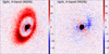 |
Fig. A.1 Qϕ and Uϕ images from the IRDAP pipeline (van Holstein et al. 2020). |
Appendix B Goodness of fit
Here we describe how we estimated the goodness of model fits by calculating χ2. For calculating probability distributions according to Bayesian Statistics, the usual total χ2 is used (see appendix D). For images, we calculate χ2 mainly for significantly detected parts of the image (see Wahhaj et al. 2021). Since the immediate background regions of any extended emission define its extent, these regions must be included in the χ2 calculation.
Accordingly, we use the regions between 10 and 75 pixels or (125 mas and 938 mas) from the star. We designate the area of this signal and background region as As + b. The noise per pixel is calculated with a typical robust sigma algorithm, and designated σ. The significant areas of detection are defined as all regions with signal twice this sigma value, which we call As. The area of a resolution element is designated Aresel, the diffraction limit at the observing wavelength or the beam size in sub-millimeter observations. Thus, our total χ2 for an image, re-scaled to reflect only the significant area is
 where i represents the pixels in As+b and fi and f′i are the data and model pixel flux, respectively. Since the sum also yields an area in pixels,
  remains a unit-less fraction as intended. We designate Nd = As/Aresel/As+b as the number of effective data points. The pixel size in the SPHERE images and our sampled ALMA images is the same. We note that c is a free scaling factor applied to the model to minimize the residual in the difference image, data−c×model, over the As+b region. Thus, the total image flux is ignored in this term; only the relative pixel-to-pixel fluxes affect
  .
.
This is because the total flux of the image has a much larger uncertainty of 15%, which is typical of relative flux calibration in comparison to the star. Thus, we calculate the total flux uncertainty separately as  , where f and f′ are the total fluxes of the data and model, respectively. Hence, the total χ2 for all our datasets which are used for probability calculations is
 where j represents the datasets ALMA 870μ , SPHERE Ks-band, SPHERE Stokes Q in H-band, etc. For best-fit searches, we use the mean reduced χ2 or
 where
where  (each dataset j has 2 parts, image and flux), since this gives better interim fits before a search has converged, as explained in the main text.
The best two-zone model parameters (Table B.1) and χ2 values (Table B.2) are presented here for completeness. The relevant discussion can be found in section 4.3.
Two-zone model best-fit parameters
Goodness-of-fit statistics for the two-zone disk model.
Appendix C Radmc3d model details
The radmc3d models are given the following resolutions in their spherical coordinate system (with coordinates, r, ϕ, θ). The radial direction is divided into two segments extending 2 to 30 au and from 30 to 200 au. Each segment is given a model resolution of 20 elements. The θ coordinate is segmented with bounds: 0, π/3, π/2 to 2π/3, and π, with resolutions of 10, 20, 20, and 10 for the respective segments. The denser regions of the model are given higher resolutions. The ϕ coordinate is given a uniform resolution of 90 elements. We use 100,000 photons and 1,000,000 scattering events. Once a good fit is found, the model is run at a higher resolution to re-check the quality of fit. The higher resolutions are 20,40 elements for r, 20,40,40 and 20 elements for θ, and 180 elements for ϕ, reported in the same order as before. This time we use 300,000 photons and 1,000,000 scattering events.
Appendix D Constraining model parameters using emcee
Here we describe our attempt to constrain the model parameters by using the Bayesian estimation python package emcee. The emcee package samples the space of model parameters (17 in the case of the three-zone disk), according to the probability of the model e−Χ2/2 using the Affine Invariant Ensemble Sampler Foreman-Mackey et al. (2013). The total χ2 is used here, as opposed to reduced χ2. This is important to note, as the relative model probability and thus the strength of the constraints is strongly influenced by the number of independent measurements, and thus the magnitude of χ2.
We used 35 parallel random walkers, each of which took 1090 steps, for a total of 38150 steps . For each walker, 242 initial steps were discounted as burn-in. The mean coherence time for walkers was ∼100 steps, but this was gradually increasing. This suggests that the probability space may be too complex, even for the adaptive EnsembleSampler routine we employed. Each model took an average of 56 s to create, and the sampler was run for 26 days to produce the constraints presented below.
Figure D.1, shows the parameter values sampled for all the walkers. General convergence is noted for all parameters, but multimodal distributions could be indicated for some. In Figure D.1, we show the probability distributions for all parameters, and the 2D probability maps for all possible pairs of the 17 parameters. Seemingly all parameters are well-constrained (see Table D.1). However, we know this to be unlikely, as some parameters are really only loosely constrained (see the large fractional error bars in Table 4). For example, the upper limit to the size of the sub-millimetergrains are not constrained by the data as explained in section 4.3. In general, the constraints found seem artificially small when compared to manual exploration of χ2 values around the local minima. Again, this is because the walkers did not complete enough steps.
Model parameter constraints from emcee.
 |
Fig. D.1 Parameter values traced by the emcee walkers. Convergence was not reached after 26 days. |
 |
Fig. D.2 Model parameter probability distributions from emcee. Convergence was not reached after 26 days. |
Appendix E Orbit fitting
In this section, we present the probability distributions of orbit fitting parameters discussed in section 3.3.
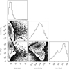 |
Fig. E.1 Probability distributions for the main orbital parameters of planet b. The 95% confidence interval is shown (see Figure 7). It seems that a circular orbit is unlikely. The inclination may still be co-planar with the disk (i ~ 49.3° or 180°–49.3° = 130.7°). |
 |
Fig. E.2 Probability distributions for all orbital parameters of planet b. The 95% confidence intervals are shown. The parameters are sma (semi-major axis), ecc (eccentricity), inc (inclination), aop (argument of periastron), pan (position angle of nodes), tau (epoch of periastron passage, which is expressed as a fraction of orbital period past a specified offset), mtot (system mass), and plx (the system parallax). |
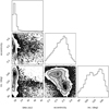 |
Fig. E.3 Probability distributions for the main orbital parameters of planet c. The 95% confidence interval is shown (see Figure Figure 7). It seems that a circular orbit is unlikely. The inclination may still be co-planar with the disk (i ~ 58.5° or 180° –58.5° = 121.5°). |
 |
Fig. E.4 Probability distributions for all orbital parameters of planet c. The 95% confidence intervals are shown. The parameters are sma (semi-major axis), ecc (eccentricity), inc (inclination), aop (argument of periastron), pan (position angle of nodes), tau (epoch of periastron passage, which is expressed as a fraction of orbital period past a specified offset), mtot (system mass), and plx (the system parallax). |
Appendix F Grain abundance ratios
In this section, we compare the grain abundance ratios between the three grain populations used in this paper. Let us consider an infinitesimal range of grain sizes, Δa, within which to count the grains. According to a single power-law size distribution (e.g., dN/da = n a−3.5; Dohnanyi 1969), the number of grains within this range is
![Mathematical equation: $\[\Delta N_i=n \, a_i^{\eta} \, \Delta a.\]$](/articles/aa/full_html/2024/07/aa49018-23/aa49018-23-eq33.png)
We note that Δa is an absolute bin size such that Δa ≪ a, but it is independent of a.1
Thus, the number ratio of the grain sizes ai and aj within a bin size Δa is given by
 (F.1)
(F.1)
Now we can compare these number ratios to the model-estimated total masses for each dust population, Mi (see Table 4):
![Mathematical equation: $\[M_i=\rho \, V_i \, \Delta N_i . \] \[\Rightarrow \Delta N_i = M_i/(\rho \, V_i) \; \propto M_i \, {a_i}^{-3}.\]$](/articles/aa/full_html/2024/07/aa49018-23/aa49018-23-eq35.png)
Here, Vi is the grain volume,  and ρ is the grain density. Thus, the ratio of the grain sizes from the model-mass estimates is
![Mathematical equation: $\[\Delta N_i/\Delta N_j = \frac{M_i}{M_j} \left(\frac{a_i}{a_j}\right)^{-3}.\]$](/articles/aa/full_html/2024/07/aa49018-23/aa49018-23-eq37.png)
Using this result in Equation F.1, we solved for η
![Mathematical equation: $\[\eta = \frac{log(M_i/M_j)}{log(a_i/a_j)}-3.\]$](/articles/aa/full_html/2024/07/aa49018-23/aa49018-23-eq38.png)
Using the estimates with upper and lower error bars in Table 4 and comparing number ratios between 0.1 and 10.9 μm grains we get η = -3.33 to -3.27, while comparing 0.1 and 300 μm grains we get η= -2.69 to -2.66. Using the equations above, we see that 10.9 μm grains are over-abundant by a factor of 2, compared to the 0.1μ grains (assuming dN/da ∝ a-3.5), while the ∼300 μmgrains are over-abundant by more than a factor of 1000. In Figure F.1, we show that the discrepancies with the dN/da ∝ a-3.5 power law are quite significant for the ∼300μm grains.
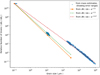 |
Fig. F.1 Model-estimated relative abundances of the three grain sizes compared to those predicted by the power law dN/da ∝ a-3.5 (Dohnanyi 1969). We used the asymmetric upper and lower uncertainties (see Table 4) to generate 3000 data pairs ai and Δ Ni in order to properly account for correlated errors. |
References
- Andrews, S. M. 2020, ARAA, 58, 483 [NASA ADS] [CrossRef] [Google Scholar]
- Bae, J., Zhu, Z., Baruteau, C., et al. 2019, APJ, 884, L41 [NASA ADS] [CrossRef] [Google Scholar]
- Baraffe, I., Chabrier, G., Barman, T. S., Allard, F., & Hauschildt, P. H. 2003, AAP, 402, 701 [NASA ADS] [CrossRef] [EDP Sciences] [Google Scholar]
- Benisty, M., Bae, J., Facchini, S., et al. 2021, APJ, 916, L2 [NASA ADS] [CrossRef] [Google Scholar]
- Benisty, M., Dominik, C., Follette, K., et al. 2023, in, ASP Conf. Ser., 534, Protostars and Planets VII, eds. S. Inutsuka, Y. Aikawa, T. Muto, K. Tomida, & M. Tamura, 605 [NASA ADS] [Google Scholar]
- Beuzit, J. L., Vigan, A., Mouillet, D., et al. 2019, AAP, 631, A155 [NASA ADS] [CrossRef] [EDP Sciences] [Google Scholar]
- Blunt, S., Nielsen, E. L., De Rosa, R. J., et al. 2017, AJ, 153, 229 [Google Scholar]
- Bruderer, S. 2013, AAP, 559, A46 [NASA ADS] [CrossRef] [EDP Sciences] [Google Scholar]
- Bruderer, S., van Dishoeck, E. F., Doty, S. D., & Herczeg, G. J. 2012, AAP, 541, A91 [NASA ADS] [CrossRef] [EDP Sciences] [Google Scholar]
- Campbell-White, J., Manara, C. F., Benisty, M., et al. 2023, APJ, 956, 25 [CrossRef] [Google Scholar]
- Claudi, R. U., Turatto, M., Gratton, R. G., et al. 2008, SPIE CONF. SER., 7014, 70143E [NASA ADS] [Google Scholar]
- Cridland, A. J., Facchini, S., van Dishoeck, E. F., & Benisty, M. 2023, AAP, 674, A211 [NASA ADS] [CrossRef] [EDP Sciences] [Google Scholar]
- de Boer, J., Langlois, M., van Holstein, R. G., et al. 2020, AAP, 633, A63 [NASA ADS] [CrossRef] [EDP Sciences] [Google Scholar]
- Dohlen, K., Langlois, M., Saisse, M., et al. 2008, SPIE CONF. SER., 7014, 70143L [NASA ADS] [Google Scholar]
- Dohnanyi, J. S. 1969, JGR, 74, 2531 [NASA ADS] [CrossRef] [Google Scholar]
- Dong, R., Hashimoto, J., Rafikov, R., et al. 2012, APJ, 760, 111 [CrossRef] [Google Scholar]
- Dorschner, J., Begemann, B., Henning, T., Jaeger, C., & Mutschke, H. 1995, AAP, 300, 503 [NASA ADS] [Google Scholar]
- Draine, B. T. 2006, APJ, 636, 1114 [NASA ADS] [CrossRef] [Google Scholar]
- Dullemond, C. P., &Dominik, C. 2004, A&A, 417, 159 [NASA ADS] [CrossRef] [EDP Sciences] [Google Scholar]
- Facchini, S., Teague, R., Bae, J., et al. 2021, AJ, 162, 99 [NASA ADS] [CrossRef] [Google Scholar]
- Foreman-Mackey, D., Hogg, D. W., Lang, D., & Goodman, J. 2013, PASP, 125, 306 [Google Scholar]
- Gagné, J., Mamajek, E. E., Malo, L., et al. 2018, APJ, 856, 23 [CrossRef] [Google Scholar]
- Grundy, W. M., Olkin, C. B., Young, L. A., et al. 2013, ICARUS, 223, 710 [NASA ADS] [CrossRef] [Google Scholar]
- Guidi, G., Isella, A., Testi, L., et al. 2022, AAP, 664, A137 [NASA ADS] [CrossRef] [EDP Sciences] [Google Scholar]
- Haffert, S. Y., Bohn, A. J., de Boer, J., et al. 2019, NAT. ASTRON., 3, 749 [NASA ADS] [CrossRef] [Google Scholar]
- Hashimoto, J., Dong, R., Kudo, T., et al. 2012, APJ, 758, L19 [NASA ADS] [CrossRef] [Google Scholar]
- Isella, A., Benisty, M., Teague, R., et al. 2019, APJ, 879, L25 [NASA ADS] [CrossRef] [Google Scholar]
- Jaeger, C., Mutschke, H., Begemann, B., Dorschner, J., & Henning, T. 1994, AAP, 292, 641 [NASA ADS] [Google Scholar]
- Juillard, S., Christiaens, V., & Absil, O. 2022, AAP, 668, A125 [NASA ADS] [CrossRef] [EDP Sciences] [Google Scholar]
- Keppler, M., Benisty, M., Müller, A., et al. 2018, AAP, 617, A44 [NASA ADS] [CrossRef] [EDP Sciences] [Google Scholar]
- Lafrenière, D., Marois, C., Doyon, R., Nadeau, D., & Artigau, É. 2007, APJ, 660, 770 [CrossRef] [Google Scholar]
- Long, Z. C., Akiyama, E., Sitko, M., et al. 2018, APJ, 858, 112 [CrossRef] [Google Scholar]
- Marois, C., Lafrenière, D., Doyon, R., Macintosh, B., & Nadeau, D. 2006, APJ, 641, 556 [CrossRef] [Google Scholar]
- Mawet, D., Milli, J., Wahhaj, Z., et al. 2014, APJ, 792, 97 [CrossRef] [Google Scholar]
- Mesa, D., Keppler, M., Cantalloube, F., et al. 2019, AAP, 632, A25 [NASA ADS] [CrossRef] [EDP Sciences] [Google Scholar]
- Milli, J., Mouillet, D., Lagrange, A. M., et al. 2012, AAP, 545, A111 [NASA ADS] [CrossRef] [EDP Sciences] [Google Scholar]
- Müller, A., Keppler, M., Henning, T., et al. 2018, AAP, 617, L2 [CrossRef] [EDP Sciences] [Google Scholar]
- Pecaut, M. J., & Mamajek, E. E. 2016, MNRAS, 461, 794 [Google Scholar]
- Portilla-Revelo, B., Kamp, I., Rab, C., et al. 2022, AAP, 658, A89 [NASA ADS] [CrossRef] [EDP Sciences] [Google Scholar]
- Powell, M. J. D. 1964, COMPUT. J., 7, 155 [CrossRef] [Google Scholar]
- Ren, B. B., Benisty, M., Ginski, C., et al. 2023, A&A, 680, A114 [NASA ADS] [CrossRef] [EDP Sciences] [Google Scholar]
- Riaud, P., Mawet, D., Absil, O., et al. 2006, AAP, 458, 317 [NASA ADS] [CrossRef] [EDP Sciences] [Google Scholar]
- Schmid, H. M., Bazzon, A., Roelfsema, R., et al. 2018, AAP, 619, A9 [NASA ADS] [CrossRef] [EDP Sciences] [Google Scholar]
- Skinner, S. L., & Audard, M. 2022, APJ, 938, 134 [NASA ADS] [CrossRef] [Google Scholar]
- Soummer, R. 2005, APJ, 618, L161 [NASA ADS] [CrossRef] [Google Scholar]
- Stolker, T., Min, M., Stam, D. M., et al. 2017, AAP, 607, A42 [NASA ADS] [CrossRef] [EDP Sciences] [Google Scholar]
- Swastik, C., Banyal, R. K., Narang, M., et al. 2021, AJ, 161, 114 [Google Scholar]
- Swastik, C., Wahhaj, Z., Benisty, M., et al 2024, A&A, submitted [NASA ADS] [CrossRef] [EDP Sciences] [Google Scholar]
- van Holstein, R. G., Snik, F., Girard, J. H., et al. 2017, SPIE CONF. SER., 10400, 1040015 [NASA ADS] [Google Scholar]
- van Holstein, R. G., Girard, J. H., de Boer, J., et al. 2020, AAP, 633, A64 [NASA ADS] [CrossRef] [EDP Sciences] [Google Scholar]
- van Holstein, R. G., Stolker, T., Jensen-Clem, R., et al. 2021, AAP, 647, A21 [NASA ADS] [CrossRef] [EDP Sciences] [Google Scholar]
- Vigan, A., Moutou, C., Langlois, M., et al. 2010, MNRAS, 407, 71 [Google Scholar]
- Wagner, K., Follete, K. B., Close, L. M., et al. 2018, APJ, 863, L8 [NASA ADS] [CrossRef] [Google Scholar]
- Wahhaj, Z., Koerner, D. W., Backman, D. E., et al. 2005, APJ, 618, 385 [CrossRef] [Google Scholar]
- Wahhaj, Z., Liu, M. C., Biller, B. A., et al. 2013, APJ, 779, 80 [CrossRef] [Google Scholar]
- Wahhaj, Z., Milli, J., Romero, C., et al. 2021, AAP, 648, A26 [NASA ADS] [CrossRef] [EDP Sciences] [Google Scholar]
- Wang, J. J., Vigan, A., Lacour, S., et al. 2021, AJ, 161, 148 [Google Scholar]
- Zhu, W., & Dong, S. 2021, ARAA, 59, 291 [NASA ADS] [CrossRef] [Google Scholar]
- Zurlo, A., Vigan, A., Mesa, D., et al. 2014, AAP, 572, A85 [NASA ADS] [CrossRef] [EDP Sciences] [Google Scholar]
This is a computational requirement set by the power law dN/da = n aγ, and not related to whether the models demand values proportionally or absolutely close to a.
All Tables
All Figures
|
Fig. 1 SPHERE Observations of PDS 70. Top row, left to right: IRDIS Ks-band, Stokes Q/H-band, and Stokes U/H-band images. Bottom row: H-, J-, and Y-band IFS observations, median combined over the typical band widths. North is up, east is left, and the black circle in the center is a mask over the coronagraphic region. |
| In the text | |
|
Fig. 2 Inverted H-band polarized fraction map given by |
| In the text | |
|
Fig. 3 IRDIS Ks-band reduction to bring out the planets by trying to remove the disk. A smoothed version of the disk reduction (median smoothed over 12 pixel boxes) along with the PSFs of the reference star was supplied to the LOCI algorithm in order to subtract both the disk and star. |
| In the text | |
|
Fig. 4 IRDIS Ks reduction to recover simulated planets and detection limits as shown in Fig. 5. The disk has been subtracted as described in the text. The real planets b and c are labeled. |
| In the text | |
|
Fig. 5 IRDIS Ks-band detection contrast limit for S/N >5 (shown with the blue curve). It was made from the simulated planet recovery, as explained in the main text. The orange line shows the limits corrected for small sample statistics according to Mawet et al. 2014. The mass detection limits are estimated from the DUSTY models, assuming an age of 5 Myr for PDS 70. The dashed line represents the detection limit at the brightest part of the disk. |
| In the text | |
|
Fig. 6 IFS observations. Top: YJH-band images made from collapsing the IFS spectra and the locations from which the planet and disk spectra were extracted. Bottom: IFS Spectra of the b and c planets along with spectra of this dust ring at three locations. The planet spectra are similar to each other, and clearly different from the disk spectra. The region contaminated by telluric absorptions around 1.4 μ is grayed out. |
| In the text | |
|
Fig. 7 Orbit fitting using astrometry from this work and earlier studies for planet b (left) and c (right). The best 500 orbits from 1 000 000 orbits fitted by the orbitize! package (Blunt et al. 2017) are shown along with predictions of separation and PA for the near future. |
| In the text | |
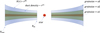 |
Fig. 8 Schematic of the model dust disk as described in Sect. 4.2. |
| In the text | |
|
Fig. 9 Comparison of Radmc3D preliminary two-zone model images with data. The figure shows poor fits to the polarimetry data. The left, middle, and right columns represent the data, model, and residual, respectively. The top, middle, and bottom rows are the Ks-band total intensity image, H-band Stokes Q image, and ALMA 870 μ image, respectively. The data and model images are of the same resolution. |
| In the text | |
|
Fig. 10 Comparison of Radmc3D three-zone model images with data. The left, middle, and right columns represent the data, model, and residual respectively. The rows from top to bottom are the Ks-band total intensity image, H-band Stokes Q image, Stokes U image, and ALMA 870 μm image, respectively. |
| In the text | |
|
Fig. 11 Comparison of Radmc3D three-zone model images with Y-, J- and H-band IFS observations, median combined over the typical band widths. For these, the models were not fitted because of computational limits. Simulated noise has been added to the data, but no planets were simulated. The data and model are morphological very similar. |
| In the text | |
|
Fig. A.1 Qϕ and Uϕ images from the IRDAP pipeline (van Holstein et al. 2020). |
| In the text | |
|
Fig. D.1 Parameter values traced by the emcee walkers. Convergence was not reached after 26 days. |
| In the text | |
|
Fig. D.2 Model parameter probability distributions from emcee. Convergence was not reached after 26 days. |
| In the text | |
|
Fig. E.1 Probability distributions for the main orbital parameters of planet b. The 95% confidence interval is shown (see Figure 7). It seems that a circular orbit is unlikely. The inclination may still be co-planar with the disk (i ~ 49.3° or 180°–49.3° = 130.7°). |
| In the text | |
|
Fig. E.2 Probability distributions for all orbital parameters of planet b. The 95% confidence intervals are shown. The parameters are sma (semi-major axis), ecc (eccentricity), inc (inclination), aop (argument of periastron), pan (position angle of nodes), tau (epoch of periastron passage, which is expressed as a fraction of orbital period past a specified offset), mtot (system mass), and plx (the system parallax). |
| In the text | |
|
Fig. E.3 Probability distributions for the main orbital parameters of planet c. The 95% confidence interval is shown (see Figure Figure 7). It seems that a circular orbit is unlikely. The inclination may still be co-planar with the disk (i ~ 58.5° or 180° –58.5° = 121.5°). |
| In the text | |
|
Fig. E.4 Probability distributions for all orbital parameters of planet c. The 95% confidence intervals are shown. The parameters are sma (semi-major axis), ecc (eccentricity), inc (inclination), aop (argument of periastron), pan (position angle of nodes), tau (epoch of periastron passage, which is expressed as a fraction of orbital period past a specified offset), mtot (system mass), and plx (the system parallax). |
| In the text | |
|
Fig. F.1 Model-estimated relative abundances of the three grain sizes compared to those predicted by the power law dN/da ∝ a-3.5 (Dohnanyi 1969). We used the asymmetric upper and lower uncertainties (see Table 4) to generate 3000 data pairs ai and Δ Ni in order to properly account for correlated errors. |
| In the text | |
Current usage metrics show cumulative count of Article Views (full-text article views including HTML views, PDF and ePub downloads, according to the available data) and Abstracts Views on Vision4Press platform.
Data correspond to usage on the plateform after 2015. The current usage metrics is available 48-96 hours after online publication and is updated daily on week days.
Initial download of the metrics may take a while.