| Issue |
A&A
Volume 687, July 2024
|
|
|---|---|---|
| Article Number | A276 | |
| Number of page(s) | 14 | |
| Section | Astrophysical processes | |
| DOI | https://doi.org/10.1051/0004-6361/202348719 | |
| Published online | 23 July 2024 | |
Role of magnetic fields in disc galaxies: spiral arm instability⋆
1
Hamburger Sternwarte, Universität Hamburg, Gojenbergsweg 112, 21029 Hamburg, Germany
e-mail: This email address is being protected from spambots. You need JavaScript enabled to view it.
2
Research School of Astronomy and Astrophysics, The Australian National University, Canberra, ACT 2611, Australia
Received:
23
November
2023
Accepted:
15
April
2024
Abstract
Context. Regularly spaced star-forming regions along the spiral arms of nearby galaxies provide insight into the early stages and initial conditions of star formation. The regular separation of these star-forming regions suggests spiral arm instability as their origin.
Aims. We explore the effects of magnetic fields on the spiral arm instability.
Methods. We use 3D global magnetohydrodynamical simulations of isolated spiral galaxies, comparing three different initial plasma β values (ratios of the thermal to magnetic pressure) of β = ∞, 50, and 10. We perform a Fourier analysis to calculate the separation of the over-dense regions that formed as a result of the spiral instability. We then compare the separations with observations.
Results. We find that the spiral arms in the hydro case (β = ∞) are unstable. The fragments are initially connected by gas streams that are reminiscent of the Kelvin-Helmholtz instability. For β = 50, the spiral arms also fragment, but the fragments separate earlier and tend to be slightly elongated in the direction perpendicular to the spiral arms. However, in the β = 10 run, the arms are stabilised against fragmentation by magnetic pressure. Despite the difference in the initial magnetic field strengths of the β = 50 and 10 runs, the magnetic field is amplified to βarm ∼ 1 inside the spiral arms for both runs. The spiral arms in the unstable cases (hydro and β = 50) fragment into regularly spaced over-dense regions. We determine their separation to be ∼0.5 kpc in the hydro and ∼0.65 kpc in the β = 50 case. These two values agree with the observed values found in nearby galaxies. We find a smaller median characteristic wavelength of the over-densities along the spiral arms of 0.73−0.36+0.31 kpc in the hydro case compared to 0.98−0.46+0.49 kpc in the β = 50 case. Moreover, we find a higher growth rate of the over-densities in the β = 50 run compared to the hydro run. We observe magnetic hills and valleys along the fragmented arms in the β = 50 run, which is characteristic of the Parker instability.
Key words: instabilities / magnetohydrodynamics (MHD) / stars: formation / ISM: magnetic fields / galaxies: ISM
Movies are available at https://www.aanda.org.
© The Authors 2024
 Open Access article, published by EDP Sciences, under the terms of the Creative Commons Attribution License (https://creativecommons.org/licenses/by/4.0), which permits unrestricted use, distribution, and reproduction in any medium, provided the original work is properly cited.
This article is published in open access under the Subscribe to Open model. This email address is being protected from spambots. You need JavaScript enabled to view it. to support open access publication.
1. Introduction
Star formation in spiral galaxies is driven by their spiral arms (Nguyen et al. 2017). Star-forming regions that resemble a beads-on-a-string pattern are ubiquitous in spiral arms of numerous nearby galaxies, even though their morphological features and physical properties are different (e.g. Elmegreen & Elmegreen 1983; Elmegreen et al. 2006). Recently, spiral arms were also seen in rings of barred (Gusev & Shimanovskaya 2020) and lenticular galaxies (Proshina et al. 2022). These star-forming regions are found to be bright in the IR (Elmegreen et al. 2006, 2018; Elmegreen & Elmegreen 2019) and at times also in the far-UV (FUV) and Hα (Efremov 2009, 2010; Gusev & Efremov 2013; Gusev et al. 2022) emission, where they trace various stages of star formation. Despite the variety in spiral galaxies that host these regular star-forming regions, the adjacent separations of these regions fall in the range 350 − 500 pc and (or) integer multiples of this range (cf. Gusev et al. 2022). For example, it was found that the adjacent separation of star-forming regions in the spiral arms of NGC 628 and M 100 were both ∼400 pc (Gusev & Efremov 2013; Elmegreen et al. 2018). Another prominent example is the north-western arm of M 31, where star complexes with a spacing of twice this value ∼1.1 kpc were found (Efremov 2009, 2010). This characteristic separation of these star-forming regions in spiral arms indicates that their origin might be through a spiral arm instability. Another interesting feature observed together with regular star-forming regions in M 31 were magnetic fields out of the plane of the galaxy, with a wavelength twice that of the adjacent separation of these regions (Efremov 2009, 2010). This indicates that magnetic fields could play an important role in the formation of these regions.
Beads-on-a-string patterns have been observed along spiral arms in numerical simulations (e.g. Chakrabarti et al. 2003; Wada & Koda 2004; Kim & Ostriker 2006; Shetty & Ostriker 2006; Wada 2008; Renaud et al. 2013). The physical mechanism responsible, however, has been debated. It was hypothesised to be the Kelvin-Helmholtz (KH) hydrodynamical instability (Wada & Koda 2004), an artefact of numerical noise (Hanawa & Kikuchi 2012) or of infinitesimally flat 2D discs (Kim & Ostriker 2006), a magnetic Jeans instability (MJI; Kim & Ostriker 2006), which was also called the feathering instability (Lee 2014), or a hydro instability along spiral shocks distinct from the KH instability, called the wiggle instability (Kim et al. 2014, WI). Its physical nature was recently established to be a combination of KHI (as proposed in Wada & Koda 2004) and a vorticity-generating instability due to repeated passages of spiral shocks (Mandowara et al. 2022). Restricting their physical setups to different physical processes, these works reported facets of the same physical instability around the spiral shock. However, we also know from 2D local simulations and linear analysis (Mandowara et al. 2022) that the spiral instability is highly non-linear and sensitive to the physical properties of the interstellar medium (ISM). This includes the sound speed (cs) and the strength of the spiral shock. One of these important factors are magnetic fields.
Even though the role of magnetic fields has been explored, the effect they can have in a global realistic setting still remains to be determined. We expect from earlier works that they can affect the length and growth scales of the instability. For example, Lee (2014) showed that the spiral shock fronts were weaker in the presence of stronger magnetic fields, and the feather instability growth rate was not affected. However, the range of their parameter space only spanned from β = 2 − 4. Kim et al. (2014) reported based on a 2D local linear analysis and simulations that equipartition magnetic fields (β = 1) in comparison with very weak fields (β = 100) decreased the growth rate of the spiral arm instability by a factor of 4 and increased the wavelength of the dominant mode by a factor of 2 and had an overall stabalising effect overall. In 3D local box simulations, Kim & Ostriker (2006) found no vorticity generating instability and attributed this to magnetic fields (β = 1, 10), but found that the spiral shocks were still unstable in the presence of self-gravity and magnetic fields. This was also confirmed in global 2D simulations in Shetty & Ostriker (2006), where equipartition magnetic field strengths prevented the pure hydro vortical instability, but the spiral arms fragmented in the presence of self-gravity despite the magnetic fields. Most of these studies were made in 2D (Lee 2014; Kim et al. 2015; Shetty & Ostriker 2006) or were local (Lee 2014; Kim et al. 2015; Kim & Ostriker 2006), and all of them were isothermal. While there are more sophisticated magnetised galaxy simulations (Dobbs & Price 2008; Khoperskov & Khrapov 2018), they have focused on the global evolution of the disc and not on the spiral arm instability. It is yet to be determined how magnetic fields affect the spiral arm instability in 3D global disc galaxy simulations, where the spiral arm instability, MJI, and also the Parker instability (Parker 1966) that arises due to the stratified nature of the medium perpendicular to the disc are resolved.
In this study, we focus on the physical effects of magnetic fields on the spiral arm instability and its impact on the spacings of the over-densities that result in the spiral arms. We perform 3D self-gravitating magnetised disc galaxy simulations that employ fitted functions for equilibrium cooling, heating, and an external spiral potential. This allows us to capture the spiral arm instability in a more realistic environment and to study the effects of magnetic fields on it. For this purpose, we built a library of simulations with varying initial magnetisation.
The paper is organised as follows: Section 2 describes our library of simulations. In Sect. 3, we compare the models with different magnetisations and focus on the basic morphology of our galaxies, the approximate timescales of the spiral arm instability, and the cloud spacings of the unstable spiral arms. We discuss the caveats of this work and the role played by magnetic fields on the spiral arm instability, and we compare them with existing observations and simulations in Sect. 4. We summarise our results in Sect. 5.
2. Methods
Our 3D magnetohydrodynamical (MHD) disc galaxy simulations have self-gravity, an external spiral potential, magnetic fields, and fitted functions for optically thin cooling and heating that include heating from cosmic and soft X-rays, the photoelectric effect, and the formation and dissociation of H2 (cf. Körtgen et al. 2019). The cooling and heating gives us a multiphase ISM consisting of the warm neutral medium (WNM), cold neutral medium (CNM), and a cold molecular medium (CMM). These form self-consistently in our simulations. The cooling and heating curve also has a thermally unstable regime, which is important for molecular cloud formation, in the density range 1 ≤ n/cm−3 ≤ 10. Our minimalist global models strike a balance by including dominant physical effects such as self-gravity, galactic shear, thermal instabilities, and magnetic fields, while at the same time avoiding complicated stochastic effects such as star formation and various feedback mechanisms. We do not study these mechanisms here because we focus on the effects of magnetic fields. We defer an investigation of the effects of feedback to a future study.
The system of equations that we solve is
 (1)
(1)
 (2)
(2)
 (3)
(3)
 (4)
(4)
![Mathematical equation: $$ \begin{aligned}&\frac{\partial }{\partial t} \left(\frac{\rho v^{2}}{2} + \rho \epsilon _{\rm int} + \frac{B^{2}}{8\pi }\right) + \nabla \cdot \left[\left(\frac{\rho v^{2}}{2} + P + \rho \epsilon _{\rm int} + \frac{B^{2}}{8\pi }\right) \cdot \boldsymbol{v} + v_{j}\mathcal{M} _{ij}\right]\nonumber \\&\qquad \qquad \quad = \frac{\rho }{m_{\rm H}} \Gamma - \left(\frac{\rho }{m_{\rm H}}\right)^{2} \Lambda (T), \end{aligned} $$](/articles/aa/full_html/2024/07/aa48719-23/aa48719-23-eq7.gif) (5)
(5)
where ρ is the density, and v, P, B are the velocity, pressure and the magnetic field of the gas. The gravitational potential of the gas and the external gravitational potential are given by Φ, Φext. mH is the mass of the hydrogen atom, and Γ, Λ are the heating and cooling rates, respectively (Koyama & Inutsuka 2002; Vázquez-Semadeni et al. 2007).  , and we use the polytropic equation of state, which gives ϵint = P/ρ(γ − 1), where γ = 5/3. These represent the ideal MHD equations, where we have neglected the magnetic diffusivity and fluid viscosity.
We use the FLASH (Fryxell et al. 2000; Dubey et al. 2008) grid-based MHD code to perform the simulations. The disc is initialised at the centre of a cuboidal box with a side length Lxy = 30 kpc in the plane of the disc and Lz = 3.75 kpc in the direction perpendicular to it. The minimum cell size of the base grid is 234 pc, that is, the base grid has a resolution of 128 × 128 × 16 cells. However, we achieve a maximum resolution corresponding to a minimum cell size of 7.3 pc by using adaptive mesh refinement (AMR) with five levels of refinement, corresponding to a maximum effective resolution of 4096 × 4096 × 512 cells, such that the local Jeans length was resolved with at least 32 grid cells (Federrath et al. 2011) for R ≥ 5 kpc. We do this in two steps. First, we use four levels of refinement for the initial 0.3 Trot (100 Myr) of the evolution. We then increase the maximum refinement level to five, which saves computational costs in the initial phases of the evolution, and allows us to achieve a higher refinement overall when the spiral arms start to develop. The initial Jeans length in our models is ∼1.8 kpc, and thus, we resolve it by two additional levels of refinement at the start. In order to avoid artificial fragmentation on the highest level of refinement due to violation of the Truelove criteria (Truelove et al. 1997), we have added an artificial pressure term that was adjusted so that the local Jeans length is resolved with at least four grid cells (Körtgen et al. 2019).
2.1. Basic setup
As in earlier studies (cf. Körtgen et al. 2018, 2019), we initialise the disc galaxies in our simulation suite by keeping the effective Toomre parameter (Qeff) constant, defined as
 (6)
(6)
where  and Σ are the epicyclic frequency and the surface density of the disc, cs is the sound speed, and va is the Alfvén speed of the medium. We do this so that all the simulations have a similar response to axisymmetric gravitational perturbations. Next, we use the scale height radial profile, H(R), from H I observations of the Milky Way (Binney & Merrifield 1998), which gives us
 (7)
(7)
where H(R) = R⊙(0.0085 + 0.01719 R/R⊙ + 0.00564(R/R⊙)2) with R⊙ = 8.5 kpc and  is the plasma-beta (ratio of the thermal to magnetic pressure) of the disc. For numerical reasons, we define the inner 5 kpc region to be gravitationally stable and keep it unresolved with Qeff = 20. We focus on the disc with R > 5 kpc, where we have the initial Qeff = 3, making the region of interest gravitationally stable to axisymmetric perturbations since Q ≥ 1. We also have pressure equilibrium at the boundaries to avoid any gas inflows and outflows for the same reason. We further apply a buffer zone of 1 kpc from the inner disc for our analysis to avoid any boundary effects.
We adopt a flat rotation curve for our galaxies, with the circular velocity in the plane of the galaxy given by
 (8)
(8)
where vc = 200 km s−1 for Milky Way-like galaxies, and Rc = 0.5 kpc is the core radius. This is the exact solution for the adopted dark matter potential,
![Mathematical equation: $$ \begin{aligned} \Phi _{\rm dm} = \frac{1}{2}v_{\rm c}^{2} \ln {\left\{ \frac{1}{R_{\rm c}^{2}} \left[R_{\rm c}^{2} + R^{2} + \left(\frac{z}{q}\right)^2 \right]\right\} }\cdot \end{aligned} $$](/articles/aa/full_html/2024/07/aa48719-23/aa48719-23-eq14.gif) (9)
(9)
We use a marginally lower value of vc = 150 km s−1 compared to the Milky Way. We do this to isolate and focus on the effects of the spiral instability from the presence of swing instabilities in a low-shear environment.
2.2. Turbulent initial conditions
In addition to the circular velocity of the disc, we add a turbulent initial velocity field with vrms = 10 km s−1 and a Kolmogorov scaling of k−5/3 on scales [50, 200] pc. The turbulent velocity field was constructed to have a natural mixture of solenoidal and compressible modes, generated with the methods described in Federrath et al. (2010), using the publicly available TurbGen code (Federrath et al. 2022). The details of the initial turbulent perturbations are not critical for our numerical experiments, and they primarily serve to break the symmetries in the idealised setup. They also ensure that the perturbations for the instabilities under investigation here develop self-consistently and are not seeded by numerical noise. After the initial turbulent seeds have decayed, the ISM turbulence is primarily driven by gas flows and spiral arm dynamics.
2.3. Magnetic field
Magnetic fields are observed in nearby disc galaxies to be roughly in equipartition with the turbulent kinetic energy and in super-equipartition with the thermal energy in the ISM (Beck 2015, and references therein). We characterise the strength of the magnetic field with the plasma-beta (β), that is, the ratio of the thermal to the magnetic pressure of the medium, which is also equal to the ratio of the thermal to magnetic energies. Our initial values are β ∈ {∞,50,10}, which represent the hydro, weak, and moderate magnetisation cases of our disc. We chose a higher value of β than observed (βobs ≤ 1) because we expect it to decrease with the dynamical evolution of the galaxy. We initialise the magnetic fields to be completely toroidal (m = 0 mode), which is the dominant mode found in galaxies (Beck et al. 2020), with a dependence on the gas density, such that B ∝ nα, where α = 0.5 (as done in Körtgen et al. 2019).
2.4. Spiral potential
For generating the spiral arms, we adopt a rigidly rotating two-armed spiral potential (Cox & Gómez 2002) with a pattern speed of 13.34 km s−1 kpc−1, which gives us a co-rotation radius of = 11.25 kpc and a pitch angle of α = 20°. Thus, the external gravitational potential can be written as
 (10)
(10)
where Φdm is the dark matter potential that provides the flat rotation curve (Eq. (9)), and Φsp is the spiral potential (cf. Eq. (8) in Cox & Gómez 2002). We chose the amplitude of the spiral such that the magnitude of the force due to the potential is ∼0.4 times that of the dark matter potential on average, analytically given by
 (11)
(11)
where ⟨fsp⟩ϕ is the azimuthal average of fsp = ∇Φsp and ⟨…⟩r denotes the radial average, taken over 6 to 11 kpc, which is our region of interest.
2.5. Simulation parameter study
Our library of simulations contains three runs having different initial magnetisations, with β ∈ {∞,50,10}, all with the same strength of the spiral arm perturbation, ℱsp = 0.4, a rotational velocity of vc = 150 km s−1, and an effective Q = 3. From Eq. (7), it follows that fixing these values leads to an initial density field that differs only slightly (by ≤2%) between the simulations with different β. The key initial parameters are summarised in Table 1, where we also list the mass-weighted average density (n), the sound speed (cs), and the magnetic field magnitude of the disc region of interest. With this parameter set, we initialise our galaxies to be marginally stable to axisymmetric gravitational instabilities, the thermal instability as well as swing instabilities. Since we have an initial Q > 1, the mid-plane density is a factor of 2 lower than the thermally unstable regime, and the shear environment is low with vc = 150 km s−1.
Initial conditions of the simulations.
3. Results
Here, we discuss the main results of our simulations. First, we describe the basic evolution of the three runs, that is, their general morphology and the timescales of the spiral arm formation and fragmentation in Sect. 3.1. In Sect. 3.2, we focus on the cases where the spiral arms fragment into over-dense regions. We also describe our method for extracting the separation of the clouds and then report them as well. We then present the physical properties of the spiral arms and the effects that magnetic fields have on them in Sect. 3.3.
3.1. Basic evolution
Here, we describe the basic morphology and evolution of our simulations. We first discuss the spiral arms that form self-consistently and then their subsequent fragmentation patterns in Sect. 3.1.1. We then quantify the timescales over which we see this evolution in Sect. 3.1.2.
3.1.1. Morphology
The basic morphology of the dense gas in our galaxy is presented in Fig. 1, where we show the projected density of the three models. The lower limit of the colour bar is chosen such that the denser and colder regions are highlighted in the simulations. The rows represent different time snapshots as indicated in the panels, and the columns represent the runs with varying magnetisation. Starting with the first row (t = 0.5 Trot), we can immediately see that the dense gas is dominantly present in the spiral arms. We can understand this simply by looking at the relevant drivers of the gas dynamics in the system. Since the rotation curve that we use is the analytical solution to the dark matter potential, it is the self-gravity, the magnetic fields, the external spiral potential, and the equilibrium cooling and heating that drive the time evolution of the gaseous disc. The spiral potential funnels the gas towards its minima. This forms the dense spiral arms in the presence of self-gravity and cooling, while the magnetic fields oppose this by magnetic pressure (Pmag = B2/8π). Moreover, since the initial parameters of the galaxy are such that it is stable to Toomre, thermal and swing instabilities, the spiral arms dominates the formation of dense gas in our galaxies. We can see the effect of magnetic fields even as the spiral arms are forming, when we compare the three runs in the first row of Fig. 1. The spiral arms are visibly more diffuse with increasing magnetisation due to the additional pressure support of the magnetic fields. As expected, this effect is more pronounced in the β = 10 case because the β of the gas is considerably larger in this case than in the β = 50 run, where the magnetic fields are sub-dominant in the initial phases of the evolution.
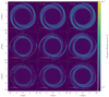 |
Fig. 1. Column density of the disc galaxies projected onto the z-plane. The columns represent the initial plasma β (ratio of thermal to magnetic pressure) of the runs, and the rows from top to bottom show the evolution of the galaxy. The panels roughly depict the times when the spiral arms first form, when the arms fragment into over-densities, and when they separate out into clouds. The disc becomes more diffuse with decreasing plasma β in the first row. The second and the third row highlight the magnetic field effects on the stability of the spiral arms. The β = 10 run is stable to fragmentation, while the hydro and β = 50 cases fragment and yet still have noticeable morphological differences. |
We begin to see major differences in the evolutionary paths of the spiral arms between the three runs after they form, as seen in the next panel at t = 0.75 Trot, where the arms start fragmenting into a beads-on-a-string pattern for the hydro and β = 50 runs, while on the other hand, the spiral arms are diffusing away in the β = 10 case. This then leads to stark differences at t = 0.9 Trot, where the spiral arms that we see at t = 0.75 Trot have distinctly separated into clouds for the hydro and β = 50 cases. While they are diffused away in the β = 10 case. Moreover, we see secondary arm formation for all the three cases, visible on the inner face of the fragmented arms in the hydro and β = 50 cases, and in the absence of a fragmented arm, solitary in the β = 10 case. We continue running the β = 10 simulation for t = 1.67 Trot and observe that the disc goes through cycles of arm formation and diffusion, and that these arms never fragment.
Now, we focus on the two runs where we see the spiral arms fragment, namely β = ∞, 50. In the Fig. 1 we can see morphological differences between the two runs at t = 0.75 Trot, even though there are no notable differences at t = 0.5 Trot, when the spiral arms form. The differences are seen in the Fig. 2, where we plot the projected density of the two runs and highlight the cells in the spiral arms with a different colour scheme to accentuate the difference. The two rows are at different times, analogous to the last two rows in Fig. 1. We trace one of the arms using a friends-of-friends (FoF) algorithm with a linking length of 60 pc, using cells that are on the verge of being thermally unstable with nthresh = 0.9 ncrit, where ncrit = 1 cm−3 is the critical density of the thermally unstable medium. In the first panel, at t = 0.75 Trot, we can see that the dense structures in the β = 50 run are all radially elongated, while the β = ∞ run has roughly sphere-shaped over-densities. The second difference is that we see wiggles that are reminiscent of Kelvin-Helmholtz instabilities, which are continuously connected with the gas in the spiral arms in the hydro run. On the other hand, the spiral arms separate out into distinct clouds without any Kelvin-Helmholtz-like structures in the runs with magnetic fields. There are differences that persist even at late times. At t = 0.9 Trot in Fig. 2 we see a larger number of fragments are more closely packed in the hydro run than in the magnetic field runs. This suggests that the fragmentation mode with magnetic fields is different from that without magnetic fields.
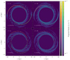 |
Fig. 2. Projected density as in Fig. 1, but only for the fragmenting cases (β = ∞ and 50). One of the arms is traced and highlighted in a different colour scheme. We can see morphological differences in the manner in which the spiral arm fragments in the presence of magnetic fields. |
3.1.2. Timescales
A more quantitative picture of the time evolution of the dense gas is presented in Fig. 3. Here, we show the time evolution of the mass-weighted average density of the gas above the density threshold for the thermally unstable regime, n > 1 cm−3. This is representative of gas that has the potential to become denser because it is in the thermally unstable regime. As expected, we find that this traced dense gas is predominantly present in the spiral arms. We visually confirm this by following the evolution of the disc with 105 passive tracer particles that are initialised at t = 0 in our region of interest (movies are provided in the supplementary material). The three solid lines in Fig. 3 are the three runs with different initial magnetisations. The stars indicate the times at which we show the disc in Fig. 1. We can separate the time evolution of the dense gas into two phases. In one phase, the spiral arms grow, and in the second phase, the gas either fragments into clouds or diffuses. The spiral arm growth phase starts at t ≃ 0.3 Trot (100 Myr) for all the runs and lasts until t ≃ 0.64 Trot (210 Myr) for the hydro and t ∼ 0.70 Trot (230 Myr) for the β = 50 run. In the β = 10 case, on the other hand, even though the spiral arms have an appreciable amount of gas around n ∼ 1 cm−3 (cf. Fig. 1), the arms never get denser. In the next phase of the evolution, the β = 10 run repeatedly forms transient arms that quickly diffuse after their formation. This phase is seen as small crests and troughs in the Fig. 3 at t ≃ 0.54, 0.74, 0.9 Trot. In contrast, the spiral arms in the other two cases fragment. This is visible as a sudden change in the slope of  in the same figure Fig. 3, which marks the end of the spiral arm growth phase. During this phase, the average density rises at a faster rate in the β = 50 case than in the hydro run. For similar time intervals from t = 230 to t = 290 Myr, the density rises by a factor of just 2.2 for the hydro run, in contrast to the factor of 5 in the magnetic run. This is seen in the steeper slope of the former compared to the latter in Fig. 3. Looking at the tracer particle movies, we see that the hydro run separates into distinct clouds at around t ≃ 290 Myr, while the β = 50 run does this much quicker by t ≃ 270 Myr.
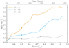 |
Fig. 3. Time evolution of the mass-weighted mean density ( |

3.2. Cloud separation and fragmentation modes
Here we discuss the difference in the separation (spacing) of the clouds that form in the spiral arms of the β = 50 case and the hydro case. This gives us insight into the effects of the magnetic fields and on the fastest-growing mode of the spiral instability.
3.2.1. Extracting the cloud spacing
We quantify the separation of the clouds and the wavelength of the unstable modes by using a 1D Fourier analysis. We do this on the projected density binned along the length of the spiral arms. We first construct a spiral arm mask using analytical functions and then use this spiral coordinate to bin the density in preparation for the Fourier transformation.
Similar to Roberts (1969), we define
 (12)
(12)
 (13)
(13)
as the spiral arm coordinates, where R0 = 1 kpc is the scaling, and p is the pitch angle of the spiral arm under consideration. The (ξ, η) coordinates can be thought of as the (lnR, θ)-plane rotated counter-clockwise by the angle p. Here, ξ is the coordinate along the spiral arm, and η is locally perpendicular to it. To define a spiral arm region of a certain thickness, we use a rectangular mask in the (ξ, η)-plane, where the thickness is decided by the extent in the η coordinate. Our spiral arm mask is shown in Fig. 4, where the first panel shows the projected density of the galaxy at t = 0.75 Trot in the (lnR, θ) plane along with the masked region (shaded) and the unit coordinate vectors  at the bottom edge of the mask. The same plot is shown in the (x, y) plane in the second panel, and the third panel shows the binned projected density along the spiral arm (coordinate ξ). We construct the mask starting with an initial guess for the pitch angle, pi, that determines the (ξ, η) plane. Next, we draw the rectangular mask in this plane that is then a rectangle bounded via fixed values of the lower edge (lnR0, θ0) and the maximum radial coordinate (lnRmax), which we determine via visual inspection at the beginning. We then test the correctness of this initial rectangular mask by fitting a straight line to all the (lnR, θ) coordinates of cells that lie in this mask, weighted by their densities. If it were a good mask that covers all the dense regions, then the slope of this line mline would be close to mi = tanpi. However, if it is not the case, we use it for the next iteration, where pi + 1 = tan−1(mi). For convergence, we use an absolute tolerance of pi + 1 − pi = 0.05°. After we construct the mask, we simply bin the projected density on the coordinate along the spiral arm.
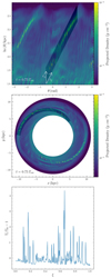 |
Fig. 4. The spiral arm mask overlaid on the column density of the disc galaxy. The first two panels show the spiral arm mask we used in the (lnR, θ) plane and in the (x, y) plane, respectively. The first panel also shows the unit vectors |

Our algorithm is similar to what Gusev & Efremov (2013) used on observational data, but with one key difference. Here, we explicitly allow for a certain thickness of the spiral arm mask in the direction perpendicular to its length, while Gusev & Efremov (2013) did not. Instead, they just fit the curve η = const. by selecting all the pixels that lay along the spiral arm by eye and determined the pitch angle p of the spiral arm via a least-squares fit.
The projected density on the coordinate along the spiral arm is shown in the bottom panel of Fig. 4. Here, the peaks in the column density are the encountered over-densities along the length of the spiral arm. We chose the number of bins such that there are ≥4 cells in each bin. With this binned density, we finally take the 1D discrete Fourier transform with the following convention:
![Mathematical equation: $$ \begin{aligned} \hat{\Sigma }_{\rm sp}[k] = \frac{1}{N} \sum ^{N-1}_{m = 0} \Sigma _{\rm sp, rel}[m] \exp {\left(\frac{-2 \pi i k m}{N}\right)}, \quad k = 0, 1, \ldots , N-1, \end{aligned} $$](/articles/aa/full_html/2024/07/aa48719-23/aa48719-23-eq23.gif) (14)
(14)
where N is the total number of bins, ![Mathematical equation: $ \Sigma_{\mathrm{sp, rel}}[m] = \Sigma_{\mathrm{sp}}[m]/\bar{\Sigma}_{\mathrm{sp}} - 1 $](/articles/aa/full_html/2024/07/aa48719-23/aa48719-23-eq24.gif) is the relative surface density along the spiral in the mth bin, and k is the wave number in units of 1/Lspiral, with Lspiral being the length of the spiral arm. We calculate Lspiral by averaging over the lengths of the inner and outer edge of the spiral arms. The power is then taken to be
is the relative surface density along the spiral in the mth bin, and k is the wave number in units of 1/Lspiral, with Lspiral being the length of the spiral arm. We calculate Lspiral by averaging over the lengths of the inner and outer edge of the spiral arms. The power is then taken to be
![Mathematical equation: $$ \begin{aligned} P[k] = \hat{\Sigma }_{\rm sp} [k] \hat{\Sigma }_{\rm sp}^{*} [k], \end{aligned} $$](/articles/aa/full_html/2024/07/aa48719-23/aa48719-23-eq25.gif) (15)
(15)
where ![Mathematical equation: $ \hat{\Sigma}_{\mathrm{sp}}^{*} [k] $](/articles/aa/full_html/2024/07/aa48719-23/aa48719-23-eq26.gif) is the complex conjugate of
is the complex conjugate of ![Mathematical equation: $ \hat{\Sigma}_{\mathrm{sp}} [k] $](/articles/aa/full_html/2024/07/aa48719-23/aa48719-23-eq27.gif) . As a final step, we bin the resultant power spectrum in bins of length k = 2.
. As a final step, we bin the resultant power spectrum in bins of length k = 2.
3.2.2. Cloud separation
We use the 1D power spectrum of the projected density derived in the last section to quantify the separation of the clouds in the spiral arms. We calculate the power spectrum at t ∈ {0.75 Trot,0.90 Trot} of one of the spiral arms as an example. These times correspond to the times shown in the bottom two panels of Fig. 2 and roughly indicate when the spiral arms are undergoing fragmentation and when the spiral arms separate into distinct clouds. The power spectrum for one of the arms is shown in Fig. 5, where the left panel shows the hydro run and the right panel the β = 50 case. The power on the vertical axis is plotted against the wave number k, which has units of 1/Lspiral, where Lspiral is the length of the spiral arm. We can see the rise in the power from t = 0.75 Trot to t = 0.90 Trot as the arm fragments and the clouds separate and become denser. This naturally produces a higher signal as the Σsp, rel grows and the spacing becomes more distinct. The hydro case has more power at early times than the β = 50 run, as expected, since it starts fragmenting t ∼ 20 Myr earlier than the latter (cf. Fig. 3). At later times, t = 0.9 Trot, we see distinct multiple peaks with similar power, where the majority of the power resides on larger scales with slight differences for both runs. For the hydro run, this is for k ≲ 80 (l ≳ 260 pc), while for the magnetic case, we have k ≲ 50 (l ≳ 390 pc).
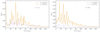 |
Fig. 5. Fourier transform of the projected density in the spiral arms for the β = ∞ and β = 50 runs. The two solid lines show the Fourier transforms at t = 0.75, 0.90 Trot, analogous to the times shown in Fig. 1. The wave number k here is given in units of 1/Lspiral, i.e., k = 1 corresponds to the full length of the spiral arm under consideration. We can see that the β = 50 run has more power at lower k (larger scales) than the hydro run, as we visually saw in Fig. 2. |
The power spectrum also gives us insights into the regularity of the separation of the clouds in this particular arm. At t = 0.90 Trot the hydro run has a major peak at k = 40 (l ∼ 500 pc). Similarly, in the β = 50 case, we see a major peak on larger scales at k = 30 (l ∼ 650 pc). They both correspond to the total number of clouds we see in the respective arms. This signal in the Fourier analysis indicates that the adjacent separations of the clouds are regular. The magnetic case also has a major peak at k = 14 (l ∼ 1.4 kpc), which corresponds to the number of brighter clouds along the spiral arm, as is also visible as the taller spikes in the bottom panel of Fig. 4.
An interesting feature in the Fourier transform common to both the runs is the presence of major peaks, which come in pairs of multiples of two. For example, we have k ∼ (24, 48), (30, 60) and (40, 80) in the hydro case and k ∼ (14, 30), (22, 44) and (34, 70) for the β = 50 case. This feature could be due to the combination of two reasons. The first is the physical presence of these modes due to the nature of the spiral arm instability, the second being the asymmetry in the negative and positive values in the function ![Mathematical equation: $ \Sigma_{\mathrm{sp, rel}}[m] = \Sigma_{\mathrm{sp}}[m]/\bar{\Sigma}_{\mathrm{sp}} - 1 $](/articles/aa/full_html/2024/07/aa48719-23/aa48719-23-eq28.gif) , of which we take the Fourier transform. In the latter case, we expect a single peak of the dominant mode followed by even harmonics with a decreasing power-law amplitude of the subsequent peaks. Looking at the lower panel of Fig. 4, we can see that the function Σ/Σ0 − 1 is indeed asymmetrical. The voids between the clouds are not as under-dense as the clouds are over-dense. However, except for the dominant modes at low k, the higher k modes all have comparable amplitudes, and we therefore consider them to be physical modes in the system.
, of which we take the Fourier transform. In the latter case, we expect a single peak of the dominant mode followed by even harmonics with a decreasing power-law amplitude of the subsequent peaks. Looking at the lower panel of Fig. 4, we can see that the function Σ/Σ0 − 1 is indeed asymmetrical. The voids between the clouds are not as under-dense as the clouds are over-dense. However, except for the dominant modes at low k, the higher k modes all have comparable amplitudes, and we therefore consider them to be physical modes in the system.
We test whether the differences observed in one of the spiral arms between the hydro and the magnetic cases can be generalised. For this, we run an identical pair of simulations for the hydro and β = 50 cases with a different random seed for the initial turbulence. We then also use both the spiral arms of each simulation in our analysis. As before, we calculate the power spectrum of the projected density along each of the arms. We show the peaks of the power spectrum in Fig. 6. Here, the error bars indicate the FWHM with a minimum value equal to the binning length k = 2 with respect to the physical scale in kpc on the horizontal axis. The left panel shows the hydro run and the right panel the β = 50 run. The different colours are for the runs with different initial turbulent seeds. The star and its error bars indicate the 50th (median) and the 16th to 84th percentile range after the points are binned in bins of 0.2 kpc.
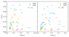 |
Fig. 6. Power (P(λ)) of the extracted peaks of the Fourier transforms of the projected density along the masked spiral arms plotted against the physical scale in kpc. The two panels show the hydro and the β = 50 cases at t = 0.9 Trot. The two runs with different random seeds are shown in yellow and blue, respectively. In each case, we have included the peaks found for the two spiral arms. The star marks the 50th percentile, and the error bars indicate the range from 16th to 84th percentile of the peaks binned in 0.2 kpc bins. It increases from |


We see from the Fig. 6 that the trends we observed in one of the spiral arms hold in the general case as well. The power in both cases exists on large scales, with the hydro run having major power over l ≳ 300 pc and the magnetic case having it on l ≳ 400 pc. We also see many significant peaks that are a multiple of 2 of a lower k mode in the magnetised and the hydro case. The rise in the cloud separation and unstable modes seen in the Fourier transform of one arm is also seen as a general trend of the presence of magnetic fields. Moreover, the power rises more steeply on small scales and also falls sharply after 1 kpc in the hydro case. For the magnetic field case, the rise in the power is shallower on smaller scales and spreads towards larger scales until 1.5 kpc. This is reflected in the percentiles of the distribution of the peaks, where the median and 16th to 64th percentile ranges of the hydro case rise from  kpc to
  kpc in the magnetised case.
3.3. Effects of the magnetic fields on the physical properties of the spiral arms
As we have seen, the magnetic fields affect the evolution of the spiral arms, regardless of their strength. The magnetic fields themselves are also expected to evolve with the gas in our simulations. In order to gain insight into this, we explore the physical properties of the spiral arms in the three different runs with different initial magnetisation before they fragment or diffuse. We use one of the spiral arms in each simulation, since we find that they have very similar physical properties. As done in Fig. 2, we trace the gas in the spiral arm under consideration at t = 0.5 Trot using a friends-of-friends algorithm with a linking length of l = 60 pc, which is the approximate cell length of the surrounding warm neutral medium around the spiral arms. In addition, we also use a density threshold of n = 0.9 cm−3, which is similar to the critical density of the thermally unstable medium. The traced spiral arms are presented in Fig. 7, where we show the projected density of the three runs along with the traced spiral arms highlighted in a different colour scheme. We use these traced regions for all the properties we report in this section.
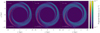 |
Fig. 7. Projected gas density of our models at t = 0.5 Trot along with the traced spiral arm highlighted with a different colour scheme. We can see that while the spiral arms in the hydro and β = 50 cases are morphologically similar to one another, there are noticeable differences with the β = 10 case. |
The total mass in the arms is similar, that is, log10(M/(M⊙) = 7.90, 7.85, and 7.71 for the hydro, β = 50, and β = 10 case, respectively. However, other physical properties vary systematically between them. We can see this in Fig. 8, where we show the mass-weighted probability density functions (PDFs) of the log10 of density in the left panel, the sound speed in the middle panel, and the cell-by-cell plasma-beta of the runs in the right panel. The stars in the histograms mark the average mass-weighted quantities in the respective vertical axis. In the left-most panel, as we saw in Sect. 3.1.2, we see that the spiral arms become more diffuse with increasing magnetisation. As seen in the mean density, which decreases by a factor of ∼2, possibly due to the additional opposing magnetic pressure. We find that the majority of the gas in the β = 10 case is present in the density range ≃1 − 3 cm−3, which is thermally unstable. Despite this, it never becomes denser because of the opposing magnetic pressure. We can also see this effect in the middle panel, where the gas in the hydro and the β = 50 cases have a lower sound speed than in the β = 10 case. This shows that the gas has already cooled in the former two cases, while it remains warm and close to its initial temperature in the latter. This is also reflected in the scale heights of the spiral arm, where the gas is found to be 50.2 ± 2.2 pc in the β = 50 case and 98.6 ± 3.9 pc in the β = 10 case. The details of the scale height calculation can be found in Appendix A. Thus the presence of magnetic fields largely causes the spiral arms to become more diffuse and hotter.
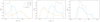 |
Fig. 8. Mass-weighted probability density functions (PDFs) of the log10 of the physical quantities of the gas in spiral arms. The left panel shows the gas density, the middle panel shows the sound speed and the right panel shows the cell-by-cell plasma-beta of the traced spiral arms at t = 0.5 Trot. The stars mark the mass-weighted average of the log10 of the quantity in each case. In the left panel, we see that the spiral arms become more diffuse with increasing magnetisation. The middle panel shows that the gas becomes colder with increasing density as the cooling sets in. In the right panel we see that, the plasma-beta of the magnetic runs have decreased significantly in the arms (compared to the simulation starting value of β), especially for the β = 50 case, where the plasma-beta has risen from 50 to an average of 2.3, becoming comparable to the β = 10 case. |
Interestingly, even though we start with a difference of a factor of 5 in the initial plasma-beta of the two magnetised runs, we note that they have similar values in the spiral arms. We see this in the right-most panel of Fig. 8, where the plasma-beta of the run with initial β = 50 has reduced by a factor of ∼25 to an average value of ∼2, and even has a non-negligible fraction of cells with values ≤1, where the magnetic fields dominate the gas pressure. The β in β = 10 run reduces by a factor of 5 to reach similar values as in the β = 50 case. This shows that the magnetic fields, even though not dynamically important at the beginning of the simulation, do become important later on in the spiral arms. This increase in field strength could be due to the combined effects of field tangling, adiabatic compression, and cooling or the presence of a dynamo (Federrath 2016). These effects are much more pronounced in the β = 50 case, where the gas compresses and cools in the absence of dynamically significant magnetic fields when compared to the β = 10 case, where they oppose compression and cooling. Thus, in the β = 50 case, we get magnetic fields that are dynamically significant after the spiral arms have become dense enough. This results in fragmentation in the presence of magnetic fields, and it changes the nature of the instability when compared with the hydro case. We discuss this in detail in the next section.
4. Discussion
Here, we discuss the physical effects of the magnetic fields on the spiral arm instability and compare them with previous theoretical and observational studies. First, we focus on the stabilising effect in Sect. 4.1, their destabilising effects in Sect. 4.2, and then go on to discuss the cloud separation and unstable modes in Sect. 4.3. Lastly, we point out some caveats of our work in Sect. 4.4.
4.1. Stabilisation
We find that moderate initial magnetic fields with an initial β = 10 can stabilise the spiral arms against fragmentation. As seen in Fig. 8, the spiral arms that form in this case are more diffuse and hotter than in the other cases (hydro and β = 50 models), where they fragment. This is mainly due to the increased magnetic pressure of the B fields that prevents the gas from becoming any denser. This inhibition of compression due to the additional magnetic pressure agrees well with other global disc galaxy simulations (Dobbs & Price 2008; Khoperskov & Khrapov 2018; Körtgen et al. 2019). However, we note that our value of β = 10 for stabilisation is higher than the values observed in other studies, β ≤ 0.1 (Dobbs & Price 2008) and β ≤ 1 (Khoperskov & Khrapov 2018). As pointed out before, our models are initially gravitationally stable and also have low shear and a warm medium.
For weak magnetic fields, β = 50, even though the spiral arms fragment, they do so in a different morphological manner than in the hydro run. The KHI-like wiggles as seen in the hydro case (reported in Wada & Koda 2004; Wada 2008; Sormani et al. 2017; Mandowara et al. 2022) are absent in the weakly magnetised simulation because the magnetic field in the spiral arms becomes dynamically important, with βarm ∼ 2, which then prevents the wiggles through magnetic tension. This stabilising effect of magnetic fields has indeed been reported for magnetic fields of near equipartition strengths in both global 2D (Shetty & Ostriker 2006) and local 3D simulations (Kim & Ostriker 2006).
4.2. Destabilisation
For the case with weak initial magnetisation, the magnetic fields rise to equipartition levels within the arm (cf. right panel of Fig. 8). However, instead of stabilising the arm, as we expect from the additional magnetic pressure, the arms still fragment. They do so by clearing out the gas within the arm into clouds ∼20 Myr before the hydro case (cf. Sect. 3.1.2). We attribute this to the possible presence of the Parker instability within the spiral arms. The Parker instability (Parker 1966, 1967a,b, 1968a,b) arises in a magnetised plasma in a stratified medium similar to that of a disc galaxy. A fluid element with a low magnetic field over-density in the disc becomes more diffuse due to the added magnetic pressure and will tend to rise upwards. Since the medium is stratified, the fluid element looses more gas after rising to adjust to the decrease in the ambient pressure, thus becoming lighter and more unstable (Shukurov & Subramanian 2021). This eventually results in a characteristic magnetic field structure of regular hills and valleys above and below the galactic plane, where clouds are expected to form in the valleys of the magnetic field lines. In our simulations, we suspect that the initial magnetic over-densities are naturally provided by the spiral arms.
To test the presence of the Parker instability, we estimated the expected growth rates and the length scales from linear theory for the gas in the spiral arms before they fragment at t = 0.50 Trot. Taking the average physical properties of the spiral arm presented in Sect. 3.3, with cs, arm = 3.55 cm s−1, βarm = 2.32, Harm = 50.2 pc, and γe = 1, we find an inverse growth rate of τ ≃ 33 Myr, and the wavelength of the fastest growing mode ≃600 pc (cf. Eqs. (17) and (22) in Mouschovias 1996). As a result of the cooling in our simulations, the gas is also expected to cool in the valleys as it becomes denser (Kosiński & Hanasz 2006; Mouschovias et al. 2009). Along with self-gravity, this is expected to increase the growth rates of the instability, which makes both the length scales and time scales remarkably close to those we observe in the spiral arms. From Fig. 3, we can roughly estimate τarm ∼ 30 Myr, and as we saw in Sect. 3.2, the cloud separation in the β = 50 runs is ≃650 pc.
In addition to this, we see the characteristic magnetic field morphology associated with the Parker instability in our spiral arms. A section of this characteristic field structure is shown at t = 0.75 Trot in Fig. 9. To produce this graph, we initialise the magnetic field lines at one yz face of the 3D box in a circular plane of radius 250 pc, coloured by the field strength. The clouds are solid iso-contours with a density of 2 cm−3, which is about twice the critical density of the thermally unstable medium. We can see the magnetic field lines rising above and below the plane of the spiral arm on scales of ∼100 pc. Since our thermally unstable medium is in the range 1 − 10 cm−3, the gas predominantly cools in the magnetic valley, as expected. Our results are in agreement with those of Mouschovias et al. (2009), who found that the Parker instability in unison with the thermal instability can lead to the formation of dense clouds in sections of spiral arms. We note here that the self-gravity, magnetic fields, and the thermal instability all act in synergy. The conditions are right for the Parker instability to play a role, but we cannot separate the non-linear interactions between the three in our simulations. In contrast to the β = 50 case, the seeds of the instability are never provided for the β = 10 case, since the spiral arms continue to disperse before they become dense enough to fragment when the field is too strong.
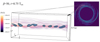 |
Fig. 9. Magnetic field lines in a section of one of the spiral arms for the β = 50 simulation at t = 0.75 Trot. The magnetic field lines, coloured by their magnitude, were initialised on the right face (yz) of the region, in a circular plane of radius 250 pc, with its z-axis aligned with that of the clouds. The clouds are shown in blue iso-contours with a threshold density of about twice the critical density of the thermally unstable medium. We can see magnetic field loops rise above and below the plane of the clouds on scales of ∼100 pc. This is an indication that the Parker instability might play a role for the spiral arm stability. |
4.2.1. Comparison to observations
One nearby galaxy, NGC 628, was recently found to show evidence of magnetic Parker loops along one of its spiral arms in RM synthesis maps (Mulcahy et al. 2017). These loops are roughly coincident with the regularly spaced star-forming regions that were studied in Gusev & Efremov (2013). A similar pattern was reported in the NW arm of M 31, where the wavelength of the Parker loops, ∼2.3 kpc (Beck et al. 1989), was found to be twice the separation of the regularly spaced star-forming regions found along the arm (Efremov 2009, 2010). These are encouraging signs of the presence of the Parker instability. However, to draw firm conclusions, more detailed analyses of a wider sample of galaxies that exhibit this regular spacing of star-forming regions along their spiral arms is needed.
4.2.2. Comparison to simulations
Linear stability analysis and local 2D simulations have observed a reduction in the growth rate of the spiral instability by a factor of 4 in the presence of equipartition magnetic fields in comparison to the hydrodynamical case (Kim et al. 2014). This is in contrast to our results, where we see an increase in the growth rates. This discrepancy could be due to their 2D approximations, in which they did not capture the onset of the Parker instability, as observed in our simulations. Kim & Ostriker (2006) observed magnetic destabilisation in their local 3D simulations of the spiral shock fronts, but attributed it to the magneto-Jeans instability (MJI), as they did not observe the characteristic Parker loops. This is not the case in our simulations probably because the spiral arms separate into clouds when the arms are at considerably low densities (nav ∼ 5 cm−3). It was also argued later that the box size of Kim & Ostriker (2006) was insufficient perpendicular to the plane of the disc to find the Parker modes (Mouschovias et al. 2009).
4.3. Cloud separation
4.3.1. Comparison to observations
Out of many others, only four spiral galaxies, namely NGC 628 (M 74), NGC 895, NGC 5474, NGC 6946, have been analysed in detail for the separation of the regularly spaced star-forming regions using a method similar to ours (Gusev & Efremov 2013; Gusev et al. 2022), where the spiral arm was parametrised in the (lnR, θ) plane. It was found that adjacent star-forming regions in all four galaxies were either at a spacing of 350 − 500 pc and/or integer multiples (2−4) of this range. This range of separations is remarkably similar to what we find, that is, ≃500 pc in the hydro and ≃650 pc in the weakly magnetised run. This is despite the differences between the parameters of our models and these galaxies.
We found that the Fourier transform of the column density along the spiral arms exhibits peaks that are integer multiples of each other (cf. Fig. 5). This effect has also been reported in all the four galaxies mentioned here (cf. Gusev et al. 2022). Since we see this in both the hydro and the weakly magnetised cases, magnetic fields are probably not the main cause for this, as previously suggested in Efremov (2010). This intriguing trend is also reflected in the strings of H I super-clouds found in the Carina arm of the Milky Way, separated by 700 pc ± 100 pc, where more massive clouds are at about twice this separation (Park et al. 2023). To draw firm conclusions from the cloud separation themselves, however, we need to expand the parameter space and tune our models to different nearby galaxies. This will help us understand the dependence of the cloud separation on the global properties of the galaxy.
4.3.2. Comparison to simulations
Other numerical works have reported an increase in the cloud separation by a factor of 2 (in local 2D simulations by Kim et al. 2015) and 3 (in local 3D simulations by Kim & Ostriker 2006) in spiral arms in the presence of magnetic fields for plasma-beta values similar to ours. This is larger than what we find, that is, an increase by a factor of 1.3 in the adjacent cloud separation as well as in the average unstable mode along the spiral arms. This could be due to the limited number statistics of the clouds in their local simulation boxes (≲10) or other limitations introduced by the local approximation, compared to global disc simulations.
4.4. Caveats
Since we focus on the effects of magnetic fields on the formation of clouds. For the sake of simplicity and computational costs, we do not include a star formation model or various feedback mechanisms, such as supernova feedback, ionising radiation, winds from massive stars, or cosmic rays. These processes might have an affect on the fragmentation process of the clouds and the structure of the spiral arms themselves. Models that include star formation and feedback will be considered in future studies. Moreover, we point out that our galaxy is isolated from its cosmological environment. Thus, we also neglect the physical effect due to fountain flows, accretion events, and mergers. Here, we focus solely on the effects of gas dynamics, which suggests that at least the onset of fragmentation of the spiral arms can be explained by self-gravity, cooling, and magnetic fields alone.
Our galaxies are gravitationally stable, have low shear (compared to the Milky Way), and initially are in the thermally stable regime. This is done to ensure that our galaxy is dominated by the spiral arms because we focus exclusively on the spiral arm instability.
5. Summary
We studied isolated spiral disc galaxies in global 3D simulations with self-gravity, magnetic fields, equilibrium heating and cooling, and an external spiral potential to study the impact of varying magnetic field strengths on the spiral arm instability. The spiral arms in our simulations form self-consistently and fragment into beads-on-a-string patterns. We found that the magnetic fields have a major dynamical impact on the spiral arm instability, which mainly depends upon their initial strength. Our conclusions are summarised below.
-
For comparable spiral background potentials, moderate initial magnetic fields (β = 10) stabilise the spiral arms against fragmentation, in contrast to the hydro and weak-field case (β = 50), where the arms are unstable. The moderate magnetic field case forms arms that are more diffuse and hotter than in the other cases due to the additional opposing magnetic pressure.
-
For the case of weak initial magnetic fields (β = 50), the spiral arms fragment in the presence of amplified equipartition magnetic fields in the arms (βarm ∼ 2.3). The magnetic tension of the fields stabilises the vortical KHI-like wiggles in the hydro case.
-
We estimate the adjacent cloud separations in the un-magnetised (hydro) case to be ∼500 pc, and ∼650 pc in the weakly magnetised case. This is remarkably close to the separations observed in many nearby spiral galaxies, which show separations of star-forming regions in the range 400−700 pc.
-
The wavelength of the average unstable mode along the spiral arms increases in length from
 kpc in the hydro case, to
  kpc in the weakly magnetised case.
 -
Additionally, the peaks of the 1D Fourier power spectrum of the column density along the spiral arms show peaks that are integer multiples of each other for both the magnetic and un-magnetised cases. This has been reported for the nearby galaxies analysed for the regularity of star-forming regions along their spiral arms.
-
The spiral arms in the weakly magnetised case separate into disjointed clouds along the arms around ∼20 Myr before the hydro case. We find indications that this may be due to the onset of the Parker instability in the spiral arms. The calculated linear growth rates and length scales of the Parker instability fall within the expected values seen in the simulation. We also showed the magnetic field morphology around the clouds in the arm that forms magnetic hills and valleys (cf. Fig. 9), as expected from linear theory.
With the advent of the James Webb Space Telescope, we can now resolve the infrared cores that are observed along the spiral arms of nearby galaxies (Elmegreen et al. 2006, 2018; Elmegreen & Elmegreen 2019) in unprecedented detail. Future parameter studies will aim to tailor our models to nearby galaxies for a more direct comparison with these observations.
Movies
Movie 1 associated with Fig. 4 (movie_hydro) Access Supplementary Material
Movie 2 associated with Fig. 4 (movie_beta50) Access Supplementary Material
Movie 3 associated with Fig. 4 (movie_beta10) Access Supplementary Material
Acknowledgments
The authors thank the anonymous referee for their constructive comments that have improved the clarity and quality of the paper. R.A. thanks Shivan Khullar and Chris Matzner for their time and insightful discussions. C.F. acknowledges funding provided by the Australian Research Council (Future Fellowship FT180100495 and Discovery Project DP230102280), and the Australia-Germany Joint Research Cooperation Scheme (UA-DAAD). We further acknowledge high-performance computing resources provided by the Leibniz Rechenzentrum and the Gauss Centre for Supercomputing (grants pr32lo, pr48pi and GCS Large-scale project 10391), the Australian National Computational Infrastructure (grant ek9) and the Pawsey Supercomputing Centre (project pawsey0810) in the framework of the National Computational Merit Allocation Scheme and the ANU Merit Allocation Scheme. The simulation software, FLASH, was in part developed by the Flash Centre for Computational Science at the Department of Physics and Astronomy of the University of Rochester.
References
- Beck, R. 2015, A&ARv, 24, 4 [Google Scholar]
- Beck, R., Loiseau, N., Hummel, E., et al. 1989, A&A, 222, 58 [NASA ADS] [Google Scholar]
- Beck, R., Chamandy, L., Elson, E., & Blackman, E. G. 2020, Galaxies, 8, 4 [Google Scholar]
- Binney, J., & Merrifield, M. 1998, Galactic Astronomy (Princeton: Princeton University Press) [Google Scholar]
- Chakrabarti, S., Laughlin, G., & Shu, F. H. 2003, ApJ, 596, 220 [NASA ADS] [CrossRef] [Google Scholar]
- Cox, D. P., & Gómez, G. C. 2002, ApJS, 142, 261 [NASA ADS] [CrossRef] [Google Scholar]
- Dobbs, C. L., & Price, D. J. 2008, MNRAS, 383, 497 [Google Scholar]
- Dubey, A., Fisher, R., Graziani, C., et al. 2008, in Numerical Modeling of Space Plasma Flows, eds. N. V. Pogorelov, E. Audit, & G. P. Zank, ASP Conf. Ser., 385, 145 [NASA ADS] [Google Scholar]
- Efremov, Y. N. 2009, Astron. Lett., 35, 507 [NASA ADS] [CrossRef] [Google Scholar]
- Efremov, Y. N. 2010, MNRAS, 405, 1531 [NASA ADS] [Google Scholar]
- Elmegreen, B. G., & Elmegreen, D. M. 1983, MNRAS, 203, 31 [NASA ADS] [Google Scholar]
- Elmegreen, B. G., & Elmegreen, D. M. 2019, ApJS, 245, 14 [NASA ADS] [CrossRef] [Google Scholar]
- Elmegreen, D. M., Elmegreen, B. G., Kaufman, M., et al. 2006, ApJ, 642, 158 [NASA ADS] [CrossRef] [Google Scholar]
- Elmegreen, B. G., Elmegreen, D. M., & Efremov, Y. N. 2018, ApJ, 863, 59 [NASA ADS] [CrossRef] [Google Scholar]
- Federrath, C. 2016, J. Plasma Phys., 82, 535820601 [Google Scholar]
- Federrath, C., Roman-Duval, J., Klessen, R. S., Schmidt, W., & Mac Low, M. 2010, A&A, 512, A81 [NASA ADS] [CrossRef] [EDP Sciences] [Google Scholar]
- Federrath, C., Chabrier, G., Schober, J., et al. 2011, Phys. Rev. Lett., 107, 114504 [NASA ADS] [CrossRef] [Google Scholar]
- Federrath, C., Roman-Duval, J., Klessen, R. S., Schmidt, W., & Mac Low, M. M. 2022, Astrophysics Source Code Library [record ascl:2204.001] [Google Scholar]
- Fryxell, B., Olson, K., Ricker, P., et al. 2000, ApJS, 131, 273 [Google Scholar]
- Gusev, A. S., & Efremov, Y. N. 2013, MNRAS, 434, 313 [CrossRef] [Google Scholar]
- Gusev, A. S., & Shimanovskaya, E. V. 2020, A&A, 640, L7 [NASA ADS] [CrossRef] [EDP Sciences] [Google Scholar]
- Gusev, A. S., Shimanovskaya, E. V., & Zaitseva, N. A. 2022, MNRAS, 514, 3953 [NASA ADS] [CrossRef] [Google Scholar]
- Hanawa, T., & Kikuchi, D. 2012, in Numerical Modeling of Space Plasma Slows (ASTRONUM 2011), eds. N. V. Pogorelov, J. A. Font, E. Audit, & G. P. Zank, ASP Conf. Ser., 459, 310 [Google Scholar]
- Khoperskov, S. A., & Khrapov, S. S. 2018, A&A, 609, A104 [NASA ADS] [CrossRef] [EDP Sciences] [Google Scholar]
- Kim, W.-T., & Ostriker, E. C. 2006, ApJ, 646, 213 [NASA ADS] [CrossRef] [Google Scholar]
- Kim, W.-T., Kim, Y., & Kim, J.-G. 2014, ApJ, 789, 68 [NASA ADS] [CrossRef] [Google Scholar]
- Kim, Y., Kim, W.-T., & Elmegreen, B. G. 2015, ApJ, 809, 33 [NASA ADS] [CrossRef] [Google Scholar]
- Kosiński, R., & Hanasz, M. 2006, MNRAS, 368, 759 [Google Scholar]
- Koyama, H., & Inutsuka, S.-I. 2002, ApJ, 564, L97 [Google Scholar]
- Körtgen, B., Banerjee, R., Pudritz, R. E., & Schmidt, W. 2018, MNRAS, 479, L40 [NASA ADS] [Google Scholar]
- Körtgen, B., Banerjee, R., Pudritz, R. E., & Schmidt, W. 2019, MNRAS, 489, 5004 [CrossRef] [Google Scholar]
- Lee, W.-K. 2014, ApJ, 792, 122 [NASA ADS] [CrossRef] [Google Scholar]
- Mandowara, Y., Sormani, M. C., Sobacchi, E., & Klessen, R. S. 2022, MNRAS, 513, 5052 [NASA ADS] [CrossRef] [Google Scholar]
- Mouschovias, T. C. 1996, in The Parker Instability in the Interstellar Medium, ed. K. C. Tsinganos (Dordrecht: Springer), 475 [Google Scholar]
- Mouschovias, T. C., Kunz, M. W., & Christie, D. A. 2009, MNRAS, 397, 14 [NASA ADS] [CrossRef] [Google Scholar]
- Mulcahy, D. D., Beck, R., & Heald, G. H. 2017, A&A, 600, A6 [NASA ADS] [CrossRef] [EDP Sciences] [Google Scholar]
- Nguyen, N. K., Pettitt, A. R., Tasker, E. J., & Okamoto, T. 2017, MNRAS, 475, 27 [Google Scholar]
- Park, G., Koo, B. C., Kim, K. T., & Elmegreen, B. 2023, ApJ, 955, 59 [NASA ADS] [CrossRef] [Google Scholar]
- Parker, E. N. 1966, ApJ, 145, 811 [NASA ADS] [CrossRef] [Google Scholar]
- Parker, E. N. 1967a, ApJ, 149, 517 [NASA ADS] [CrossRef] [Google Scholar]
- Parker, E. N. 1967b, ApJ, 149, 535 [NASA ADS] [CrossRef] [Google Scholar]
- Parker, E. N. 1968a, ApJ, 154, 49 [NASA ADS] [CrossRef] [Google Scholar]
- Parker, E. N. 1968b, ApJ, 154, 57 [NASA ADS] [CrossRef] [Google Scholar]
- Proshina, I. S., Moiseev, A. V., & Sil’chenko, O. K. 2022, Astron. Lett., 48, 139 [NASA ADS] [CrossRef] [Google Scholar]
- Renaud, F., Bournaud, F., Emsellem, E., et al. 2013, MNRAS, 436, 1836 [NASA ADS] [CrossRef] [Google Scholar]
- Roberts, W. W. 1969, ApJ, 158, 123 [NASA ADS] [CrossRef] [Google Scholar]
- Shetty, R., & Ostriker, E. C. 2006, ApJ, 647, 997 [Google Scholar]
- Shukurov, A., & Subramanian, K. 2021, Astrophysical Magnetic Fields: From Galaxies to the Early Universe, Cambridge Astrophysics (Cambridge: Cambridge University Press) [CrossRef] [Google Scholar]
- Sormani, M. C., Sobacchi, E., Shore, S. N., Treß, R. G., & Klessen, R. S. 2017, MNRAS, 471, 2932 [NASA ADS] [CrossRef] [Google Scholar]
- Truelove, J. K., Klein, R. I., McKee, C. F., et al. 1997, ApJ, 489, L179 [CrossRef] [Google Scholar]
- Vázquez-Semadeni, E., Gómez, G. C., Jappsen, A. K., et al. 2007, ApJ, 657, 870 [CrossRef] [Google Scholar]
- Wada, K. 2008, ApJ, 675, 188 [NASA ADS] [CrossRef] [Google Scholar]
- Wada, K., & Koda, J. 2004, MNRAS, 349, 270 [Google Scholar]
Appendix A: Scale height estimation
We estimate the scale height around the spiral arms by quantifying the density as a function of the z-coordinate, which is perpendicular to the plane of the galactic disc. We take the spiral arms traced via the friends-of-friends (FoF) algorithm (cf. Section 3.3). For each (x,y) in the arms, we define z = 0 as the point of maximum density. This ensures that we trace the spiral arms in three dimensions. We then bin the density in bins of 20 pc. This is shown in Figure A.1, where the density is plotted on the vertical axis and the z-coordinate on the horizontal axis. For the scale height calculation, we then fit the functional form ρ(z) = ρ0exp( − |z|/H) to the binned data. The fits are shown as dotted lines in Figure A.1. This gives us ρ0 and the scale height H. The scale heights are found to be 50.2 ± 2.2 pc for the β = 50 case and 98.6 ± 3.9 pc for the β = 10 case.
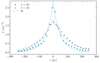 |
Fig. A.1. Gas density as a function of the z-coordinate around the traced spiral arms at t = 0.50 Trot. The fit is of the functional form ρ(z) = ρ0exp( − |z|/H). |
All Tables
All Figures
|
Fig. 1. Column density of the disc galaxies projected onto the z-plane. The columns represent the initial plasma β (ratio of thermal to magnetic pressure) of the runs, and the rows from top to bottom show the evolution of the galaxy. The panels roughly depict the times when the spiral arms first form, when the arms fragment into over-densities, and when they separate out into clouds. The disc becomes more diffuse with decreasing plasma β in the first row. The second and the third row highlight the magnetic field effects on the stability of the spiral arms. The β = 10 run is stable to fragmentation, while the hydro and β = 50 cases fragment and yet still have noticeable morphological differences. |
| In the text | |
|
Fig. 2. Projected density as in Fig. 1, but only for the fragmenting cases (β = ∞ and 50). One of the arms is traced and highlighted in a different colour scheme. We can see morphological differences in the manner in which the spiral arm fragments in the presence of magnetic fields. |
| In the text | |
|
Fig. 3. Time evolution of the mass-weighted mean density ( |
| In the text | |
|
Fig. 4. The spiral arm mask overlaid on the column density of the disc galaxy. The first two panels show the spiral arm mask we used in the (lnR, θ) plane and in the (x, y) plane, respectively. The first panel also shows the unit vectors |
| In the text | |
|
Fig. 5. Fourier transform of the projected density in the spiral arms for the β = ∞ and β = 50 runs. The two solid lines show the Fourier transforms at t = 0.75, 0.90 Trot, analogous to the times shown in Fig. 1. The wave number k here is given in units of 1/Lspiral, i.e., k = 1 corresponds to the full length of the spiral arm under consideration. We can see that the β = 50 run has more power at lower k (larger scales) than the hydro run, as we visually saw in Fig. 2. |
| In the text | |
|
Fig. 6. Power (P(λ)) of the extracted peaks of the Fourier transforms of the projected density along the masked spiral arms plotted against the physical scale in kpc. The two panels show the hydro and the β = 50 cases at t = 0.9 Trot. The two runs with different random seeds are shown in yellow and blue, respectively. In each case, we have included the peaks found for the two spiral arms. The star marks the 50th percentile, and the error bars indicate the range from 16th to 84th percentile of the peaks binned in 0.2 kpc bins. It increases from |
| In the text | |
|
Fig. 7. Projected gas density of our models at t = 0.5 Trot along with the traced spiral arm highlighted with a different colour scheme. We can see that while the spiral arms in the hydro and β = 50 cases are morphologically similar to one another, there are noticeable differences with the β = 10 case. |
| In the text | |
|
Fig. 8. Mass-weighted probability density functions (PDFs) of the log10 of the physical quantities of the gas in spiral arms. The left panel shows the gas density, the middle panel shows the sound speed and the right panel shows the cell-by-cell plasma-beta of the traced spiral arms at t = 0.5 Trot. The stars mark the mass-weighted average of the log10 of the quantity in each case. In the left panel, we see that the spiral arms become more diffuse with increasing magnetisation. The middle panel shows that the gas becomes colder with increasing density as the cooling sets in. In the right panel we see that, the plasma-beta of the magnetic runs have decreased significantly in the arms (compared to the simulation starting value of β), especially for the β = 50 case, where the plasma-beta has risen from 50 to an average of 2.3, becoming comparable to the β = 10 case. |
| In the text | |
|
Fig. 9. Magnetic field lines in a section of one of the spiral arms for the β = 50 simulation at t = 0.75 Trot. The magnetic field lines, coloured by their magnitude, were initialised on the right face (yz) of the region, in a circular plane of radius 250 pc, with its z-axis aligned with that of the clouds. The clouds are shown in blue iso-contours with a threshold density of about twice the critical density of the thermally unstable medium. We can see magnetic field loops rise above and below the plane of the clouds on scales of ∼100 pc. This is an indication that the Parker instability might play a role for the spiral arm stability. |
| In the text | |
|
Fig. A.1. Gas density as a function of the z-coordinate around the traced spiral arms at t = 0.50 Trot. The fit is of the functional form ρ(z) = ρ0exp( − |z|/H). |
| In the text | |
Current usage metrics show cumulative count of Article Views (full-text article views including HTML views, PDF and ePub downloads, according to the available data) and Abstracts Views on Vision4Press platform.
Data correspond to usage on the plateform after 2015. The current usage metrics is available 48-96 hours after online publication and is updated daily on week days.
Initial download of the metrics may take a while.