| Issue |
A&A
Volume 698, June 2025
|
|
|---|---|---|
| Article Number | L6 | |
| Number of page(s) | 6 | |
| Section | Letters to the Editor | |
| DOI | https://doi.org/10.1051/0004-6361/202554886 | |
| Published online | 27 May 2025 | |
Letter to the Editor
Gravitational instability and spatial regularity of the gas clouds and young stellar population in spiral arms of NGC 628
1
Sternberg Astronomical Institute, Lomonosov Moscow State University, Universitetsky Pr. 13, 119234 Moscow, Russia
2
Central (Pulkovo) Astronomical Observatory, Russian Academy of Sciences, Pulkovskoye Chaussee 65/1, 196140 St. Petersburg, Russia
3
Saint Petersburg State University, 7/9 Universitetskaya Nab., St. Petersburg 199034, Russia
⋆ Corresponding authors: This email address is being protected from spambots. You need JavaScript enabled to view it.
, This email address is being protected from spambots. You need JavaScript enabled to view it.
Received:
31
March
2025
Accepted:
2
May
2025
Abstract
Context. There is a clear contradiction between the characteristic spacings in observed regular chains of star-forming regions in the spiral arms of galaxies (∼500 pc) and the estimates of the wavelength of gravitational instability in them (> 1 kpc).
Aims. We aim to calculate the scales of regularity in the grand-design galaxy NGC 628 in terms of gravitational instability by using modern high-quality observational data and comparing them with scales of spatial regularity of the star-forming regions and molecular clouds in the spiral arms of the galaxy.
Methods. We investigated two mechanisms of gravitational instability against radial and azimuthal perturbations in a multicomponent disk with a finite thickness. We obtained a map of the instability wavelength distribution and compared its median value with the typical scale of observed regularity.
Results. The maps of instability parameters Q and S, which are related to the radial and azimuthal perturbations, respectively, show a good alignment between gravitationally unstable regions and areas of recent star formation. By analyzing the distribution of giant molecular clouds along the spiral arms of NGC 628, we found a similar regularity of about 500−600 pc that had previously been observed for star-forming regions. Additionally, the distribution of the wavelength most unstable to azimuthal perturbations yields a median value of about 700 pc, which is close to the observed scale regularity. This latter finding helps resolve the discrepancy between theoretically predicted and observed scales of star-forming regions in terms of regularity.
Key words: hydrodynamics / instabilities / galaxies: individual: NGC 628 / galaxies: kinematics and dynamics / galaxies: spiral
© The Authors 2025
 Open Access article, published by EDP Sciences, under the terms of the Creative Commons Attribution License (https://creativecommons.org/licenses/by/4.0), which permits unrestricted use, distribution, and reproduction in any medium, provided the original work is properly cited.
This article is published in open access under the Subscribe to Open model. This email address is being protected from spambots. You need JavaScript enabled to view it. to support open access publication.
1. Introduction
Turbulence compression and gravitational collapse are believed to play a key role in the creation and evolution of molecular clouds and their descendants, namely, star-forming (SF) regions. The sizes and spatial distribution of gaseous (H2 and H I) clouds and SF regions in galactic disks can be explained in terms of gravitational or magneto-gravitational instability (see e.g. Elmegreen 1994a).
Elmegreen & Elmegreen (1983) were the first to find regular strings of H II regions in spiral arms of galaxies. They noted the rarity of this phenomenon, as merely 10% of grand design galaxies studied have visually detectable regular chains of H II regions, with typical distances between adjacent regions of 1−4 kpc across different galaxies. The regularity in the distribution of H2 clouds and SF regions implies the constancy of a number of physical parameters of the interstellar medium (ISM) and stellar population in the stellar-gaseous disk on sufficiently large scales within the disk and across a wide range of galactocentric distances; notably, this is not expected to typically occur in typical galactic disks. Indeed, theoretical studies of the gravitational instability of gaseous, stellar-gaseous, multicomponent disks (Safronov 1960; Elmegreen & Elmegreen 1983; Jog & Solomon 1984; Romeo & Falstad 2013; Romeo & Mogotsi 2017; Rafikov 2001), as well as the study of the fragmentation of gas filaments, along with single- and multicomponent spiral arms and rings (Inutsuka & Miyama 1997; Mattern et al. 2018; Elmegreen 1994a,b; Inoue & Yoshida 2018) predict regularities on scales of a few kpc for typical values of parameters of the ISM and stellar medium (Elmegreen & Elmegreen 1983; Marchuk 2018; Inoue et al. 2021).
However, in the last decade, regular and quasiregular chains of SF regions and gas clouds in spiral arms and rings have been discovered in many galaxies of various morphological types, from S0 to Scd, as well as in the Carina Arm of the Milky Way (MW), with a characteristic spacing equal to (or a multiple of) 350−500 pc (Gusev & Efremov 2013; Elmegreen et al. 2018; Henshaw et al. 2020; Gusev & Shimanovskaya 2020; Gusev et al. 2022; Proshina et al. 2022; Park et al. 2023). Recent magnetohydrodynamic simulations in a MW-like galaxy carried out by Arora et al. (2024) also offered a prediction of the formation of regular chains of gas clouds in spiral arms on scales of ∼500 pc in the hydrodynamic case (and slightly more in the magnetic case). Meidt et al. (2023) found subkiloparsec characteristic distances between gas filaments and similar turbulent Jeans lengths in four galaxies, including NGC 628, using PHANG–JWST data. Thus, recent studies have reshaped our understanding of the prevalence of the regularity phenomenon and its characteristic spatial scales.
Despite the recently published results from Meidt et al. (2023) and Arora et al. (2024), the question of an agreement between observational data (demonstrating a scale of ∼500 pc) and theoretical models (scale of > 1 kpc) remains open. The aim of this Letter is to directly calculate the scales of regularity in galaxies in terms of gravitational instability, using modern high-quality surveys, which provide the necessary observational data (parameters of the ISM and stellar population, and disk kinematics).
As an object of study, we chose the well-known nearby galaxy NGC 628 (M74), which is viewed almost face-on (Fig. 1). It is a prototype of the grand-design galaxy, in which Gusev & Efremov (2013) found regular chains of SF regions in both spiral arms of the galaxy with spacing of ≈550 pc (for the distance 10 Mpc).
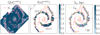 |
Fig. 1. Left and center panels: Maps of instability parameters related to radial (Q) and azimuthal (S) perturbations, calculated from the minimum value of the corresponding component of the stellar velocity dispersion. Right panel: Distribution of instability wavelengths relative to azimuthal perturbations, λϕ. The red contours on the left indicate isolines of Hα brightness, with values of logHα equal to −17.2 and −16.5 [erg/s/cm2]. Red and orange contours in the middle and right panels correspond to logHα = −17.2 [erg/s/cm2] and ΣH2 = 30 M⊙/pc2. |
2. Mechanisms of gravitational instability
In this Letter, we investigate two distinct mechanisms of gravitational instability that may regulate the large-scale star formation process in galaxies. Both mechanisms involve the assumption of the coexistence of gas and stellar components in a disk with a finite thickness. The first mechanism was considered in Rafikov (2001) based on an analysis of the axisymmetric stability of a rotating disk. To take into account the influence of both components, rather than using the hydrodynamical approximation, as was done in Wang & Silk (1994), Rafikov (2001) examined the instability process more accurately by using the collisionless Boltzmann equation for a stellar disk. As a result, the following expression for the instability parameter was derived:
![Mathematical equation: $$ \begin{aligned} \frac{1}{Q(\overline{k_r})}=\frac{2}{Q_{\rm s}}\frac{1}{\overline{k_r}}\left[1-e^{-\overline{k_r}^{2}} I_{0}(\overline{k_r^2})\right]+\frac{2}{Q_{\rm g}}\frac{\overline{k_r}s}{1+\overline{k_r^2}s^{2}}, \end{aligned} $$](/articles/aa/full_html/2025/06/aa54886-25/aa54886-25-eq1.gif) (1)
(1)
where Qs = 𝜘σsr/πGΣs and Qg = 𝜘σgr/πGΣg are classical instability parameters for stellar and gaseous disks (Toomre 1964),  and s = σgr/σsr. In the above equations, Σs and Σg represent the surface densities of stars and gas; meanwhile, 𝜘 and I0 – the epicyclic frequency and the modified Bessel function of the first kind; σg, sr are the radial components of the gas and stellar velocity dispersion; and kr is a wave number of radial perturbations. We assumed that the disk has a finite thickness and we modified the stability criterion by adding a multiplier Fg, s(k) to each term in Eq. (1), where Fg, s is equal to
 ![Mathematical equation: $ [{1 - \exp(-k h_{\mathrm{g,s}}^{z})]}/{[k h_{\mathrm{g,s}}^{z}}] $](/articles/aa/full_html/2025/06/aa54886-25/aa54886-25-eq3.gif) , while hg, sz represents the typical vertical scales of the gas and stellar components (similarly to Jog & Solomon 1984; Elmegreen 1995).
, while hg, sz represents the typical vertical scales of the gas and stellar components (similarly to Jog & Solomon 1984; Elmegreen 1995).
Another mechanism examined in this Letter considers the formation of giant clumps in tightly wound spirals that rotate with constant pattern speed, Ωp (Inoue & Yoshida 2018, 2019). The authors examined azimuthal perturbations in the spiral arms, whose radial slice profile was assumed to be described by a Gaussian function with a peak value Σ0 at R0 and dispersion w. The derived instability parameter takes the following form:
 (2)
(2)
In Eq. (2) g, s = 1.4 W Σ0 represents a linear mass of a certain slide of spiral with half-width of W ≈ 1.55w for gaseous and stellar components; f(kϕlg, s) is a linear combination of modified Bessel and Struve functions, as described in Inoue & Yoshida (2018), depending on the wave number of the perturbation, kϕ, and the distance from the spiral ridge, l. We note that in this case, σg, sϕ represents the azimuthal projections of the gas and stellar velocity dispersions.
The formal criteria for gravitational instability in both mechanisms state that if the minimum values of the Q(kr) and S(kϕ) functions are less than 1, then a particular region of the disk is unstable to radial or azimuthal perturbations accordingly. We note that the value of λr, ϕ = 2π/kr, ϕ (at which kr, ϕ leads to the minimum of these functions) is considered to be the wavelength of the most unstable radial or azimuthal perturbation mode.
3. Data and methods
We examine the process of gravitational instability using the example of the grand-design spiral galaxy NGC 628. We assumed the inclination, i, and positional angle, PA, to be 7° and 25°, respectively. The distance to NGC 628 is still a subject of debate. There are two alternative estimates of the distance to the galaxy: 7.2 Mpc (see e.g. Sharina et al. 1996; Van Dyk et al. 2006) and 9.3−10 Mpc (see e.g. Hendry et al. 2005; Olivares et al. 2010). We adopted the distance of 10 Mpc in this Letter; however, in Appendix A we compare our obtained results for two distances: 10 Mpc and 7.2 Mpc.
We assumed that the gas component of the disk consists of neutral HI and molecular hydrogen H2. The map of the surface density, ΣHI, was obtained from THINGS (Walter et al. 2008) data and estimated using the standard conversion (see Eq. 2 from Yıldız et al. 2017). For the gas velocity dispersion, we took the HI result obtained from THINGS. Additionally, we assumed this quantity to be isotropic, so its azimuthal and radial projections are equal to the extracted σg value. The vertical scale of the gas disk was defined from the vertical equilibrium condition as hg = σg2/(πGΣg).
Since direct observations of cold molecular hydrogen in external galaxies are not trivial, it is common to estimate its abundance by observing the CO line. Using modern observational data of CO(J = 2 − 1) from ALMA (Leroy et al. 2021), we estimated the surface density of H2 as  , where R21 ≈ 0.65 is the ratio of the CO(J = 2 − 1) to CO(J = 1 − 0) lines (den Brok et al. 2021). To calculate
  , we used Eq. (14) from Chiang et al. (2023), which includes the distribution of the stellar mass and metallicity (taken from Williams et al. 2022).
Regarding the stellar component of the disk, we focused on obtaining surface density using near-infrared observations, as this relates to the old population of stars that make up the majority of the galactic stellar mass and determine its potential. We used Spitzer data at 3.6 μm and 4.5 μm bands (Sheth et al. 2010) and estimated Σs using Eq. (8) from Querejeta et al. (2015). For the stellar velocity dispersion, we followed a similar approach to that described in Marchuk & Sotnikova (2017), Marchuk (2018), which allowed us to place limits on the radial (σsr) and azimuthal (σsϕ) components of velocity dispersion based on the observational line-of-sight data σlos from VLT MUSE (Emsellem et al. 2022). That way, knowing that according to observations (see Pinna et al. 2018; Walo-Martín et al. 2021) and numerical models (Sotnikova & Rodionov 2003), the σsz/σsr ratio lies in the range of 0.5 ÷ 0.8, we can use σφ/σr = 𝜘/(2Ω), which is the epicyclic approximation (Binney & Tremaine 2008), along with the stellar velocity ellipsoid equation to estimate, for example, the radial projection of σs at a certain polar angle φ:
where m = 0.52, 0.82 are taken for  ,
,  , respectively. The azimuthal component was derived from the radial one using the epicyclic approximation. The aforementioned epicyclic frequency and angular velocity were taken from the velocity rotation curve approximation, based on THINGS data presented in Marchuk (2018). To estimate the vertical scale, hs, we used the length scale taken from Leroy et al. (2008) and the ratio between the scale length and height q = 7.3 (Kregel et al. 2002).
To extract the linear mass of each radial slice of the spiral arms, we first determined the edges of two spirals using the method described in Savchenko et al. (2020). We then fit a Gaussian function to each slice extracted from the Σg and Σs maps. As a result, we derived the surface density at the peak, Σ0, and the width of the spiral arm, W, for each component, which allows us to obtain the linear mass g and s. We note, by fixing the location R0 where Σ takes its peak value, we can also determine the distance to the spiral ridge, l. Following Inoue et al. (2021), the edges of each arm at a certain slice were defined as the location where Σ = 0.3Σ0 and the minimum l cannot be less than the spatial resolution. Then, Ωp was estimated using corotation resonance measurements. According to Kostiuk et al. (2024), this galaxy may have two patterns rotating at 52 and 30 km/s/kpc.
All the aforementioned data images were rebinned to a THINGS pixel size of 1.5 arcsec/pix and cropped by the field of view defined by ALMA and MUSE images. In addition, the data were also convolved with a THINGS beam size of 6.8 arcsec and 5.57 arcsec, which corresponds to a spatial resolution of approximately 150 pc at a distance of 10 Mpc.
Additionally, to the study of the distribution of SF regions in spiral arms of NGC 628 obtained in Gusev & Efremov (2013), we explored the distribution of H2 clouds along the spiral arms of the galaxy, based on the CO(J = 2 − 1) map from ALMA (Leroy et al. 2021). We used a technique developed in Gusev & Efremov (2013) and Gusev & Shimanovskaya (2020). It includes along-arm photometry, finding distances Δs between adjacent local maxima of brightness on the CO flux profiles along every arm, along with an analysis of their distributions, computing the Lomb-Scargle periodograms (Scargle 1982) for the function p(s), where p(s) is a collection of Gaussians centered at points of local maxima of brightness on the profiles, with σ equal to the peak positioning error. To obtain photometric profiles along spiral arms, we used the same elliptical aperture (40 × 6 arcsec2) with a minor axis along a spiral arm and a step of 1° by PA as in Gusev & Efremov (2013). Preliminarily, two main CO spiral arms were fitted with a logarithmic spiral with the same pitch angle, 15.7°, same as the angle used for the stellar spiral arms in Gusev & Efremov (2013).
4. Results and discussion
Figure 1 (see the left and central panels) shows maps of the gravitational instability parameters Q and S (minimum of functions from Eqs. 1 and 2) derived from the minimum values of radial and azimuthal components of σs, respectively. The maximal estimates of these parameters exceed the minimum ones by no more than a factor of 1.5 and they still indicate the same regions of instability (i.e., where Q < 1 or S < 1). Each image contains isolines of the Hα brightness (MUSE/VLT) shown with the red contours, which indicate regions with recent (< 10 Myr) star formation. In most non-central areas, these contours remarkably correspond to regions gravitationally unstable to both radial and azimuthal perturbations (dotted hatching). In the central regions, star formation can be predicted by taking into account other types of perturbations that lead to an increased threshold value of the instability parameters up to 1.5−3 (Morozov 1985; Griv & Gedalin 2012; Zasov & Zaitseva 2017). Thus, we have demonstrated that for most areas in spirals, the parameter Q corresponds to an unstable regime, implying the ability of the disk to fragment. The S map also shows gravitational instability in arms, primarily in gaseous clouds filled with molecular hydrogen.
While a similar analysis of gravitational instability for NGC 628 was previously conducted by Marchuk (2018) and Inoue et al. (2021), our examination has led to quite different results. For instance, with respect to the instability parameter map presented in the central panel of Fig. 1, Inoue et al. (2021) showed spiral-arm regions with higher values of S > 1, predicting a stable state. We believe this significant difference primarily relates to the divergent methods used for estimating certain quantities, particularly the surface density of H2 and old stars and the stellar velocity dispersion. In contrast to the findings of Marchuk (2018), our study reports lower values of the Q parameter, apparently due to the use of more recent data from ALMA and MUSE and more accurate estimations.
According to Gusev & Efremov (2013), NGC 628 has regularly spaced SF regions forming a chain-like structure along spiral arms, with a range of separations spanning ∼500−600 pc (assuming D = 10 Mpc). This feature of NGC 628 is not unique, but it is rather common to other galaxies (see Gusev 2023, and references therein). There have been several attempts to reconcile the observed spacings in the regular chains of SF regions with theoretical calculations of the gravitational instability scales (see our introduction), although no definitive answer has been found thus far. In the present study, we have aimed to solve this puzzle by examining the mechanism of spiral arm instability, which predicts the formation of clumps. In particular, we focus on the distribution of wavelengths of the most unstable azimuthal perturbation mode. A similar approach was performed in Meidt et al. (2023) to explain a quasi-regular spacing of filaments by considering Jeans and Toomre wavelengths. The right panel of Fig. 1 shows the map of λϕ derived from the wavenumber, kϕ, which corresponds to the minimum of the function S(kϕ). This image shows that for most spiral pattern areas with recent star formation (red contour), the wavelength of instability lies within 0.5 ÷ 1 kpc (dotted hatches), which is consistent with the regularity spacing found in Gusev & Efremov (2013). In addition, the magnitude of λϕ related to the instability regions does not vary essentially along the arms, supporting the existence of regularity.
In addition to the separation between SF regions obtained in Gusev & Efremov (2013), we analyzed the distribution of local maxima of CO brightness indicating the location of giant molecular clouds (GMC). The middle panel of Fig. 2 shows two peaks, similar for both arms. The main peak contains two-thirds of separations in the range from 420 to 720 pc, with a mean of  pc in both arms. The secondary peak contains the remaining one-third of the separations in the range of 840−1020 pc with a
  pc. The characteristic separations of the main peak for H2 clouds are in good agreement with the results presented in the top panel for SF regions obtained by Gusev & Efremov (2013),
  pc (adopted for D = 10 Mpc). The Fourier analysis data support the presence of the spatial regularity of local maxima of CO brightness on the same scales (see solid lines at the bottom panel of Fig. 2). The periodograms have noticeable peaks at 680 pc with a false-alarm probability (FAP) < 45% for spiral 1 and 480, 640 pc with FAP < 5% for arm 2. Despite the fact that the peak for spiral 1 has a high FAP of ≈45% (and could possibly be false), the results of the Fourier analysis rather support the estimation of typical separations of local maxima of brightness in the arms found based on their distributions for at least one of the arms.
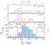 |
Fig. 2. Top and middle panels: Histograms of the distance distributions between neighboring SF regions and giant molecular clouds for different spiral arms. Bottom panel: Distribution of instability wavelengths, which are shown on the right side of Fig. 1. The blue histogram includes only those pixels with both ΣH2 > 30 M⊙/pc2 and |

The bottom panel of Fig. 2 shows the distribution of wavelengths for azimuthally unstable regions. In addition, we considered areas where the H2 surface density is greater than 30 M⊙/pc2. This is because, according to Fig. 3, at this threshold, the median value of the instability parameter S becomes near 1. The maximum of the λϕ distribution is approximately 700 pc (the median is 720 pc), which is close to the characteristic separations of the GMCs in both arms found using Fourier analysis. These values are slightly larger than the typical separations obtained from the histogram analysis. We note that the simulations of Arora et al. (2024) yielded similar results: they predicted the formation of regular chains of SF regions in spiral arms on scales of ∼500 pc in the hydro case (without a magnetic field) and ∼650 pc in the magnetic case. However, they also found a lower median characteristic wavelength of the over-densities along spiral arms, with ∼730 pc in the hydro case and ∼1.0 kpc in the magnetic one using Fourier analysis methods.
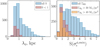 |
Fig. 3. Left panel: Distribution of wavelength, λϕ, for all regions (in blue) and for those with S < 1 (in red). The right panel: Distribution of the instability parameter S for all pixels (in blue) and for those regions with H2 surface densities greater than 30 M⊙/pc2 (in red) and 40 M⊙/pc2 (in yellow). |
It is worth noting that the use of current gas and other parameter distributions is not entirely adequate for examining the gravitational instability regime leading to the observable distribution of star formation. Although it is nearly impossible to restore the exact distribution of matter and its kinematics prior to the collapse of the observed GMCs, we can consider two boundary cases that approximate conditions at those times. The first approach assumes the uniform distribution of gas by mass along the crest of the spiral arms. According to numerical simulations by Inoue & Yoshida (2018) and Arora et al. (2024), this condition precedes the fragmentation into regularly spaced clamps that occurs within 200−300 Myr. The second way to approximate the distribution of gas prior to clouds collapse is to smooth and average the current maps of gas density with the smoothing scale equal to the product of the free-fall collapse time and the typical velocity dispersion of gas. We assumed a velocity dispersion of 10 km/s and a collapse time of 30 Myr (the upper limit of times taken from Chevance et al. 2020; Sun et al. 2022); therefore, the smoothing scale is about 300 pc. For other parameters, we assume that their distributions undergo negligible changes over such short timescales. According to Fig. 4, the case with an equal gas distribution demonstrates stability (S ≫ 1) almost everywhere; however, for regions with a near-unstable regime, typical wavelengths are around 1 kpc or less. In contrast, the second approximation (bottom panel) shows almost the same λϕ histogram, as in Fig. 2 (bottom), with a slightly increased median value. The fact that calculated for different conditions, the characteristic instability wavelength remains within the same limits can also be proven by the similar scales of regularity found separately for GMCs and young stellar clusters (see Fig. 2).
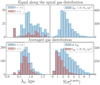 |
Fig. 4. Same histograms as in Fig. 3, calculated for a gas density that is uniformly distributed along the spiral crest (top) and for an averaged gas map with a smoothing length of 300 pc (bottom). |
To summarize, we have demonstrated that both instability mechanisms considered in this study can regulate the large-scale star formation process. Moreover, we were able to match the observed scale of regularity in SF regions and GMCs distributions with the theoretically predicted instability wavelength. As mentioned above, the typical regularity spacing obtained in previous investigations was a few kiloparsecs, which was significantly greater than the observable one. We believe this discrepancy might occur due to the greater magnitude of the instability parameters revealed in those studies. This is supported by Fig. 3, where the wavelengths of scales less than a kiloparsec mainly correspond to an unstable regime, where the parameter S < 1.
5. Conclusions
We examined the parameters of gravitational instability in NGC 628, referring to radial and azimuthal perturbations, including both gas and stellar components in a disk with finite thickness. A similar analysis has already been conducted for this galaxy; however, the use of recent data from MUSE and ALMA, as well as more accurate estimations of certain quantities, allows us to demonstrate a good agreement between theoretical predictions for the star formation locations and the observable ones. In addition, based on the mechanism assuming spiral arm fragmentation due to azimuthal perturbation, we obtained the wavelength of instability and compared it with the scale of the spacing among SF regions. Our conclusions are summarized as follows.
-
We demonstrated that locations with recent star formation traced by Hα are in good agreement with locations where the parameter Q < 1 implies gravitational instability against axisymmetric perturbations.
-
The map of the instability parameter S, related to azimuthal perturbations, shows areas with unstable regime that are consistent with the locations of gaseous clouds and SF regions.
-
We show that the spatial distribution of GMCs along the spiral arms follows a regular pattern, with a characteristic scale of 500−600 pc that matches that of SF regions.
-
When considering the instability wavelength distribution, we find that its median value (≈700 pc) is close to the observed scale of regularity.
Thus, using the example of NGC 628, we have apparently managed to remove the contradiction between the observed characteristic spacings in regular chains of SF regions and GMCs (∼0.5 − 0.6 kpc) and earlier calculations of the gravitational instability wavelength (> 1 kpc).
Acknowledgments
We are grateful to the referee for his/her constructive comments. The authors would like to thank Natalia Ya. Sontikova for her useful comments and valuable feedback on the interpretation of the findings, which improved this study. The study was conducted under the state assignment of Lomonosov State Moscow University. VK thanks the Theoretical Physics and Mathematics Advancement Foundation “BASIS” grant number 23-2-2-6-1.
References
- Arora, R., Federrath, C., Banerjee, R., & Körtgen, B. 2024, A&A, 687, A276 [NASA ADS] [CrossRef] [EDP Sciences] [Google Scholar]
- Binney, J., & Tremaine, S. 2008, Galactic Dynamics: Second Edition (Princeton: Princeton University Press) [Google Scholar]
- Chevance, M., Kruijssen, J. M. D., Hygate, A. P. S., et al. 2020, MNRAS, 493, 2872 [NASA ADS] [CrossRef] [Google Scholar]
- Chiang, I.-D., Hirashita, H., Chastenet, J., et al. 2023, MNRAS, 520, 5506 [CrossRef] [Google Scholar]
- den Brok, J. S., Chatzigiannakis, D., Bigiel, F., et al. 2021, MNRAS, 504, 3221 [NASA ADS] [CrossRef] [Google Scholar]
- Elmegreen, B. G. 1994a, ApJ, 433, 39 [NASA ADS] [CrossRef] [Google Scholar]
- Elmegreen, B. G. 1994b, ApJ, 425, L73 [NASA ADS] [CrossRef] [Google Scholar]
- Elmegreen, B. G. 1995, MNRAS, 275, 944 [NASA ADS] [CrossRef] [Google Scholar]
- Elmegreen, B. G., & Elmegreen, D. M. 1983, MNRAS, 203, 31 [NASA ADS] [Google Scholar]
- Elmegreen, B. G., Elmegreen, D. M., & Efremov, Y. N. 2018, ApJ, 863, 59 [NASA ADS] [CrossRef] [Google Scholar]
- Emsellem, E., Schinnerer, E., Santoro, F., et al. 2022, A&A, 659, A191 [NASA ADS] [CrossRef] [EDP Sciences] [Google Scholar]
- Griv, E., & Gedalin, M. 2012, MNRAS, 422, 600 [NASA ADS] [CrossRef] [Google Scholar]
- Gusev, A. S. 2023, Astron. Rep., 67, 458 [Google Scholar]
- Gusev, A. S., & Efremov, Y. N. 2013, MNRAS, 434, 313 [CrossRef] [Google Scholar]
- Gusev, A. S., & Shimanovskaya, E. V. 2020, A&A, 640, L7 [NASA ADS] [CrossRef] [EDP Sciences] [Google Scholar]
- Gusev, A. S., Shimanovskaya, E. V., & Zaitseva, N. A. 2022, MNRAS, 514, 3953 [NASA ADS] [CrossRef] [Google Scholar]
- Hendry, M. A., Smartt, S. J., Maund, J. R., et al. 2005, MNRAS, 359, 906 [NASA ADS] [CrossRef] [Google Scholar]
- Henshaw, J. D., Kruijssen, J. M. D., Longmore, S. N., et al. 2020, Nat. Astron., 4, 1064 [CrossRef] [Google Scholar]
- Inoue, S., & Yoshida, N. 2018, MNRAS, 474, 3466 [Google Scholar]
- Inoue, S., & Yoshida, N. 2019, MNRAS, 485, 3024 [NASA ADS] [CrossRef] [Google Scholar]
- Inoue, S., Takagi, T., Miyazaki, A., et al. 2021, MNRAS, 506, 84 [NASA ADS] [CrossRef] [Google Scholar]
- Inutsuka, S.-I., & Miyama, S. M. 1997, ApJ, 480, 681 [NASA ADS] [CrossRef] [Google Scholar]
- Jog, C. J., & Solomon, P. M. 1984, ApJ, 276, 114 [NASA ADS] [CrossRef] [Google Scholar]
- Kostiuk, V. S., Marchuk, A. A., & Gusev, A. S. 2024, Res. Astron. Astrophys., 24, 075007 [Google Scholar]
- Kregel, M., van der Kruit, P. C., & de Grijs, R. 2002, MNRAS, 334, 646 [NASA ADS] [CrossRef] [Google Scholar]
- Leroy, A. K., Walter, F., Brinks, E., et al. 2008, AJ, 136, 2782 [Google Scholar]
- Leroy, A. K., Schinnerer, E., Hughes, A., et al. 2021, ApJS, 257, 43 [NASA ADS] [CrossRef] [Google Scholar]
- Marchuk, A. A. 2018, MNRAS, 476, 3591 [NASA ADS] [CrossRef] [Google Scholar]
- Marchuk, A. A., & Sotnikova, N. Y. 2017, MNRAS, 465, 4956 [NASA ADS] [CrossRef] [Google Scholar]
- Mattern, M., Kainulainen, J., Zhang, M., & Beuther, H. 2018, A&A, 616, A78 [NASA ADS] [CrossRef] [EDP Sciences] [Google Scholar]
- Meidt, S. E., Rosolowsky, E., Sun, J., et al. 2023, ApJ, 944, L18 [CrossRef] [Google Scholar]
- Morozov, A. G. 1985, Soviet Astron., 29, 120 [Google Scholar]
- Olivares, E. F., Hamuy, M., Pignata, G., et al. 2010, ApJ, 715, 833 [NASA ADS] [CrossRef] [Google Scholar]
- Park, G., Koo, B.-C., Kim, K.-T., & Elmegreen, B. 2023, ApJ, 955, 59 [NASA ADS] [CrossRef] [Google Scholar]
- Pinna, F., Falcón-Barroso, J., Martig, M., et al. 2018, MNRAS, 475, 2697 [NASA ADS] [CrossRef] [Google Scholar]
- Proshina, I. S., Moiseev, A. V., & Sil’chenko, O. K. 2022, Astron. Lett., 48, 139 [NASA ADS] [CrossRef] [Google Scholar]
- Querejeta, M., Meidt, S. E., Schinnerer, E., et al. 2015, ApJS, 219, 5 [NASA ADS] [CrossRef] [Google Scholar]
- Rafikov, R. R. 2001, MNRAS, 323, 445 [NASA ADS] [CrossRef] [Google Scholar]
- Romeo, A. B., & Falstad, N. 2013, MNRAS, 433, 1389 [NASA ADS] [CrossRef] [Google Scholar]
- Romeo, A. B., & Mogotsi, K. M. 2017, MNRAS, 469, 286 [NASA ADS] [CrossRef] [Google Scholar]
- Safronov, V. S. 1960, Ann. Astrophys., 23, 979 [NASA ADS] [Google Scholar]
- Savchenko, S., Marchuk, A., Mosenkov, A., & Grishunin, K. 2020, MNRAS, 493, 390 [NASA ADS] [CrossRef] [Google Scholar]
- Scargle, J. D. 1982, ApJ, 263, 835 [Google Scholar]
- Sharina, M. E., Karachentsev, I. D., & Tikhonov, N. A. 1996, A&AS, 119, 499 [NASA ADS] [CrossRef] [EDP Sciences] [Google Scholar]
- Sheth, K., Regan, M., Hinz, J. L., et al. 2010, PASP, 122, 1397 [Google Scholar]
- Sotnikova, N. Y., & Rodionov, S. A. 2003, Astron. Lett., 29, 321 [Google Scholar]
- Sun, J., Leroy, A. K., Rosolowsky, E., et al. 2022, AJ, 164, 43 [NASA ADS] [CrossRef] [Google Scholar]
- Toomre, A. 1964, ApJ, 139, 1217 [Google Scholar]
- Van Dyk, S. D., Li, W., & Filippenko, A. V. 2006, PASP, 118, 351 [Google Scholar]
- Walo-Martín, D., Pérez, I., Grand, R. J. J., et al. 2021, MNRAS, 506, 1801 [CrossRef] [Google Scholar]
- Walter, F., Brinks, E., de Blok, W. J. G., et al. 2008, AJ, 136, 2563 [Google Scholar]
- Wang, B., & Silk, J. 1994, ApJ, 427, 759 [NASA ADS] [CrossRef] [Google Scholar]
- Williams, T. G., Kreckel, K., Belfiore, F., et al. 2022, MNRAS, 509, 1303 [Google Scholar]
- Yıldız, M. K., Serra, P., Peletier, R. F., Oosterloo, T. A., & Duc, P.-A. 2017, MNRAS, 464, 329 [Google Scholar]
- Zasov, A. V., & Zaitseva, N. A. 2017, Astron. Lett., 43, 439 [Google Scholar]
Appendix A: Instability parameters in the case of alternative distance
We examined the distribution of instability wavelengths and regular spacing of GMCs for a distance of 7.2 Mpc (see Fig. A.1, red histogram and red lines). As we can see from this figure, both theoretical and observed λ decrease with distance. Indeed, the distance between GMCs is lower for D = 7.2 Mpc proportionally to the ratio of both distances. Both the instability wavelength’s magnitude and the value of the instability parameter itself do not directly depend on distance, since the only quantities that are linked to the distance are the angular speed of the pattern and the typical vertical scale. Nevertheless, the median of the λϕ distribution (530 pc) matches the characteristic separation seen in periodograms (shown on the top), which suggests that the revealed result is not dependent on distance. However, it is worth noting the decreased number of pixels in the red histogram, which indicates that lower distance assumptions lead to stabilization of the spiral arms matter against azimuthal perturbations. This can be explained by the fact that for lower distances, the spiral pattern is rotating faster, apparently preventing the compression of gas clouds implying star formation. In addition, the higher pattern speed can cause gravitationally bound clouds to split into smaller parts, leading to decreasing wavelength values.
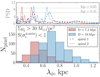 |
Fig. A.1. Top: Same periodograms as in Fig. 2. The dashed and dotted lines indicate different spiral arms. Bottom: Same distribution as at the bottom of Fig. 2. Colors of the lines and histograms indicate the distance to the galaxy used in the calculations, with red representing 7.2 Mpc and blue representing 10 Mpc. |
All Figures
|
Fig. 1. Left and center panels: Maps of instability parameters related to radial (Q) and azimuthal (S) perturbations, calculated from the minimum value of the corresponding component of the stellar velocity dispersion. Right panel: Distribution of instability wavelengths relative to azimuthal perturbations, λϕ. The red contours on the left indicate isolines of Hα brightness, with values of logHα equal to −17.2 and −16.5 [erg/s/cm2]. Red and orange contours in the middle and right panels correspond to logHα = −17.2 [erg/s/cm2] and ΣH2 = 30 M⊙/pc2. |
| In the text | |
|
Fig. 2. Top and middle panels: Histograms of the distance distributions between neighboring SF regions and giant molecular clouds for different spiral arms. Bottom panel: Distribution of instability wavelengths, which are shown on the right side of Fig. 1. The blue histogram includes only those pixels with both ΣH2 > 30 M⊙/pc2 and |
| In the text | |
|
Fig. 3. Left panel: Distribution of wavelength, λϕ, for all regions (in blue) and for those with S < 1 (in red). The right panel: Distribution of the instability parameter S for all pixels (in blue) and for those regions with H2 surface densities greater than 30 M⊙/pc2 (in red) and 40 M⊙/pc2 (in yellow). |
| In the text | |
|
Fig. 4. Same histograms as in Fig. 3, calculated for a gas density that is uniformly distributed along the spiral crest (top) and for an averaged gas map with a smoothing length of 300 pc (bottom). |
| In the text | |
|
Fig. A.1. Top: Same periodograms as in Fig. 2. The dashed and dotted lines indicate different spiral arms. Bottom: Same distribution as at the bottom of Fig. 2. Colors of the lines and histograms indicate the distance to the galaxy used in the calculations, with red representing 7.2 Mpc and blue representing 10 Mpc. |
| In the text | |
Current usage metrics show cumulative count of Article Views (full-text article views including HTML views, PDF and ePub downloads, according to the available data) and Abstracts Views on Vision4Press platform.
Data correspond to usage on the plateform after 2015. The current usage metrics is available 48-96 hours after online publication and is updated daily on week days.
Initial download of the metrics may take a while.