© The Authors 2024

1 Introduction

Earth’s atmospheric turbulence significantly affects light propagation through it, distorting both intensities and wavefronts. Consequently, ground-based astronomical observations often produce images that are more blurred than those obtained from space using identical telescopes and instruments.

Atmospheric turbulence results from stochastic fluctuations in the refractive index attributed to temperature variations. The strength of this turbulence can be quantified using the refractive index structure parameter ($C_n^2$), which is a function of the position. The Kolmogorov model provides a satisfactory description of the statistical properties of atmospheric turbulence, assuming that it is homogeneous and isotropic (e.g., Roddier 1981). This model pictures the turbulence as a cascade of energy, following a power-law distribution, from large- to small-scale turbulence eddies until dissipation. The Kolmogorov model applies only to the inertial range between the inner (ℒ₀) and outer (ℒ₀) scales determined by the smallest and largest sizes of turbulence eddies. This model holds for any atmospheric turbulence layer that light passes through on its way to the pupil entrance of ground-based telescopes, each characterized by a $C_n^2$ and an ℒ₀ that depends on the local conditions at each layer height (h). Hence, the wavefront of the light reaching the telescope pupil is affected by perturbations from the distinct atmospheric turbulence layers. We can define the spatial coherence wavefront outer scale (${ℒ}_0$) as an equivalent outer scale determining the image quality (IQ) of any observation taken with that telescope (Borgnino 1990); ${ℒ}_0$ is related to the ℒ₀ of the atmospheric turbulence layers as follows (e.g., Abahamid et al. 2004): $${ℒ}_0={\left(\frac{\int {ℒ}_0(h{)}^{-1/3}{C}_N^2(h)\mathrm{d}h}{\int C_N^2(h)\mathrm{d}h}\right)}^{-3}.$$(1)

The parameter ${ℒ}_0$ is independent of the wavelength of the observed light, representing a size and typically measured in meters. In many applications, equations are simplified by assuming infinite outer scales. Under this assumption, the full width at half maximum (FWHM) of the point spread function (PSF) in a long-exposure (LE) image, captured with a ground-based telescope limited by atmospheric turbulence, commonly referred to as the seeing-limited IQ (ε_LE), can be expressed in terms of the strength of atmospheric turbulence as $${ϵ}_{\mathrm{L}\mathrm{E}}(\lambda )\approx {ϵ}_0(\lambda )=\frac{0.976\lambda }{r_0(\lambda )},$$(2)

where ε₀ is the seeing, λ is the wavelength, and r₀ is the Fried parameter, defined in terms of the refractive index structure constant profile with height (${\mathrm{C}}_N^2$(h)) as (Fried 1965) $${\mathrm{r}}_0(\lambda )=0.185{\lambda }^{6/5}(\cos \zeta {)}^{3/5}{(\int {\mathrm{C}}_N^2(h)\mathrm{d}h)}^{-3/5},$$(3)

with ζ being the observing zenith angle. We note that Eq. (3) implies that $${ϵ}_{\mathrm{L}\mathrm{E}}(\lambda )\approx {ϵ}_0(\lambda )\propto {\lambda }^{-1/5}.$$(4)

However, interferometric measurements and the increase in size of telescope pupils show the limitations of applying the Kolmogorov model for large distances (i.e., ${ℒ}_0$ ≈ ∞), showing deviations from Eq. (4) that reveal the finite nature of the ${ℒ}_0$. Hence, with the increasing diameter of ground-based telescopes and adaptive optics (AO) developments, the relevance of ${ℒ}_0$ has increased in the last few years (e.g., Fusco et al. 2020). For example, the size of ${ℒ}_0$ strongly impacts the low-order modes in AO applications, showing a significant tilt attenuation even for pupil sizes much smaller than ${ℒ}_0$. The validity of the Kolmogorov theory beyond the inertial range can be assessed using empirical models. These models describe the spectrum of the refractive-index fluctuations by means of the ${ℒ}_0$ parameter based on general physical considerations (e.g., Voitsekhovich 1995). A widely used model was developed by von Kármán, where the ${ℒ}_0$ corresponds to the distance at which the structure-function of the phase fluctuations saturates (see, e.g., Fig. 2 in Voitsekhovich 1995).

Different techniques allow the magnitude of ${ℒ}_0$ to be determined either directly (e.g., GSM, Ziad et al. 2000) or indirectly (e.g., from AO telemetry and applying Eq. (1) in Guesalaga et al. 2017), and both provide comparable results (see Ziad 2016, for a review). At a telescope focal plane, the effect of a finite ${ℒ}_0$ is to smooth low spatial frequency perturbations, resulting in a reduction of image motion compared to that expected for an infinite ${ℒ}_0$ (e.g., Winker 1991). As a result, the actual IQ improves over the ε₀ by a factor that depends on both the ${ℒ}_0$ and the ε₀. Tokovinin (2002) proposed the following first-order approximation to ε_LE: $${ϵ}_{\mathrm{L}\mathrm{E}}(\lambda )\approx {ϵ}_0(\lambda )\sqrt{1-2.183{\left(\frac{{\mathrm{r}}_0(\lambda )}{{ℒ}_0}\right)}^{0.356}}.$$(5)

This approach results from an analytical simplification of the turbulence statistics using the von Kármán model, and it seems to work with an uncertainty of about 1% for ${ℒ}_0$/r₀ > 20. Equation (5) was refined later (Sarazin 2017) to account for the pupil size relative to ${ℒ}_0$, as $${ϵ}_{\mathrm{L}\mathrm{E}}(\lambda ,\mathcal{D})\approx {ϵ}_0(\lambda )\sqrt{1-2.183(1-\frac{1}{1+300\times \frac{\mathcal{D}}{{ℒ}_0}}){\left(\frac{{\mathrm{r}}_0(\lambda )}{{ℒ}_0}\right)}^{0.356}},$$(6)

where $\mathcal{D}$ is the telescope pupil diameter. Previous studies have adopted these analytical expressions to analyze the deviation of IQ from ε₀ using numerical simulations (Martinez et al. 2010) and through simultaneous visible and infrared images taken with different instruments (Tokovinin et al. 2007). Moreover, Floyd et al. (2010) derived an average turbulence ${ℒ}_0$ of 25 m for the Las Campanas Observatory by applying Eq. (5) to a large series of IQ measurements from band filter images of stars. Currently, first-class astronomical observatories commonly use Eq. (5) (or 6, depending on the telescope) to predict the IQ of their queue observations using the ε₀ provided by differential image motion monitors (DIMMs, Sarazin & Roddier 1990), and assuming a typical ${ℒ}_0$ for the site. However, to our knowledge, the actual ε_LE behavior with wavelength has not been verified empirically to follow such analytical approaches.

In this work we take advantage of integral field spectroscopic observations limited by atmospheric turbulence to track the wavelength behavior of the IQ at the telescope focal plane. We compare our findings with the analytical model predictions proposed by Tokovinin (2002) to determine the prevailing ε₀ during observations. We applied the methodology to data from the Multi-Unit Spectroscopic Explorer (MUSE¹) at the Paranal Observatory, empirically validating the analytical model predictions with wavelength. Thanks to the spectral range covered by MUSE, our analysis reveals the prevailing ε₀ and ${ℒ}_0$ parameters that most closely match the IQ measurements. We explored different conditions, including those influenced by dome-induced turbulence.

The structure of this article is as follows. In Sec. 2 we discuss the factors influencing IQ at the focal plane of a ground-based telescope, with special attention to dome-induced turbulence. Section 3 introduces integral field spectroscopy (IFS) as a valuable technique for assessing the ${ℒ}_0$ during observations. In Sec. 4, we apply the proposed methodology to data cubes observed with MUSE, and analyze different scenarios. Finally, in Sec. 5 we summarize the main findings and present our conclusions.

2 Telescopes and turbulence contributors

The IQ at the focal plane of an instrument attached to a ground-based telescope results from various factors, including the telescope or instrument optics and stability, and the air turbulence conditions during observations. Through this work, we use the FWHM of the PSF to quantify the IQ, although other metrics might also be employed, such as the Strehl ratio in AO applications. Modern telescopes were designed to minimize optical and stability aspects, while advanced AO systems primarily compensate for atmospheric turbulence and small optical aberrations. However, air turbulence depends on environmental conditions both inside and outside of the telescope enclosure. We identify the external turbulence to the atmospheric turbulence, assuming that Eqs. (5) and (6) describe its effect on IQ (see Appendix A for a comparison of predictions from these equations). The influence of turbulence within the telescope enclosure is complex and challenging to parameterize. We explore it further in the following subsection. Hereafter, we assume an optimal optical design of the telescope + instrument system providing negligible image degradation in comparison to air turbulence.

The dome-seeing

Telescope enclosures provide protection from external factors such as adverse weather conditions, but they can also induce turbulence, called dome-seeing (ε_dome), that degrades the quality of the images. While ε_dome is recognized as a variable source of IQ degradation, only recent efforts actively promote its monitoring, even aiming for real-time quantification (Lai et al. 2019; Stubbs 2021; Osborn & Alaluf 2023). However, there is a limited quantitative understanding of ε_dome, particularly concerning its wavelength behavior.

The non-Kolmogorov regime of the dome turbulence combines thermal inversion and convection, and its strength depends on factors such as the dome design, the inside-outside temperature gradient, the temperature of the primary mirror surface, the outside wind, and the orientation of the dome window, among others (Woolf 1979; Henry et al. 1987; Munro et al. 2023). We can define ${\tilde{r}}_0$ as an equivalent parameter to Fried’s parameter, which will be a power law of the wavelength and the non-Kolmogorov refractive index structure constant (${\tilde{C}}_N^2$) for the dome turbulence: $${\tilde{\mathfrak{r}}}_0(\lambda )={(\frac{16.7}{\cos \zeta \times {\lambda }^2}\int {\tilde{C}}_N^2\mathrm{d}h)}^{1/(2-\gamma )}.$$(7)

Here the power-law index in the range 3 < γ < 4 (Toselli et al. 2007). We note that Eq. (7) reduces to the Kolmogorov case (i.e., Eq. (3)) when $\gamma =\frac{11}{3}\approx 3.67$. Assuming that the ε_dome varies in proportion to the relationship between ε₀ and r₀ in Eq. (2), and taking into account Eq. (7): $${ϵ}_{\text{dome }}(\lambda )\propto \frac{\lambda }{{\tilde{r}}_0(\lambda )}\stackrel{(7)}{⟹}{ϵ}_{\text{dome }}(\lambda )\propto {\lambda }^{(\gamma -4)/(\gamma -2)}.$$(8)

Considering the dome’s contribution to turbulence as an additional atmospheric layer, we can linearly combine the dome-induced turbulence using the corresponding refractive index structure constants. Nevertheless, the resulting image blur from dome-turbulence could only be added to atmospheric ε₀ using a 5/3 power law within the constraints of the Kolmogorov regime (Woolf 1979; Racine et al. 1991). However, the effect of ε_dome on the focal plane is typically represented as a Gaussian blur (e.g., Bustos & Tokovinin 2018), making a quadratic contribution to the overall IQ: $$[\mathrm{IQ}(\lambda ){]}^2={[{ϵ}_{\mathrm{L}\mathrm{E}}(\lambda )]}^2+{[{ϵ}_{\text{dome }}(\lambda )]}^2.$$(9)

We have considered a negligible degradation of the IQ due to instrumental factors, and adopt such a quadratic approach hereafter. Figure 1 presents examples of the quadratic contribution to IQ for the extreme values of the power-law γ-index of the non-Kolmogorov dome-induced turbulence, assuming a ε_dome of 0.2 arcsecs at 5000 Å. We also include the $\gamma =\frac{11}{3}$ corresponding to the Kolmogorov regime. The dome contribution remains constant with wavelength as the γ-index approaches 4, whereas it becomes inversely proportional to wavelength as γ approaches 3. As shown in Fig. 1, the IQ consistently exceeds that associated with atmospheric turbulence at any wavelength. Furthermore, its wavelength dependence deviates from the natural atmospheric turbulence behavior (described by Eqs. (5) and (6)), which is particularly noticeable for the smallest γ value.

Large telescopes invest significant efforts to mitigate the occurrence of dome-induced turbulence (i.e., ε_dome ≈ 0), thereby ensuring seeing-limited conditions, and consequently, IQ ≈ ε_LE. Then, we can reasonably assume negligible or minimal ε_dome contributions at any wavelength for large telescopes. Nonetheless, the monitoring of ε_dome at distinct wavelengths will largely benefit the characterization of the actual IQ at the focal plane.

3 Using integral field spectroscopy to reveal ${ℒ}_0$

Integral field spectroscopy is a powerful technique that can perform the simultaneous recording of spatial and spectral information over a field. Since its first applications in astronomy in the 1980s and 1990s, IFS rapidly grew in popularity during the first decade of the 21st century. IFS has become a widely used technique in both ground-based and space-borne astronomy and has enabled many scientific programs, from studies in our Solar System to high-redshift objects of cosmological interest. Some of the most advanced IFS instruments in operation at the largest ground-based telescopes include the MUSE spectrograph on the Very Large Telescope (VLT) in Chile, the Gemini Multi-Object Spectrograph (GMOS²) on the Gemini Observatory in Chile and Hawaii, the Keck Cosmic Web Imager (KCWI³) on the Keck Observatory in Hawaii, and the Multi-Espectrógrafo en GTC de Alta Resolución para Astronomía (MEGARA⁴) on the Gran Telescopio Canarias on the Roque de los Muchachos Observatory in La Palma island (Spain).

The basic instrumental concept behind IFS is to spatially split the telescope’s focal plane into several subapertures, rebinning them to create a pseudo-slit to feed on long-slit spectrographs. Different instrumental approaches achieve IFS (see, e.g., Fig. 1 in Allington-Smith 2006), all of which provide the flux density (F) over a sky area in three dimensions (3D): right ascension (α), declination (δ), and wavelength (i.e., F(α,δ,λ)), under the same instrumental and atmospheric conditions. For this work the F(α,δ,λ) data cube should be viewed as a collection of narrowband filter images at different wavelengths obtained simultaneously, ensuring data homogeneity (see, e.g., Fig. 2.1 in Harrison 2016). This set of images allows us to empirically assess the variation in IQ with wavelength by characterizing the PSF using any point-like source in the observed field of view (for the initial exploration of this concept, see García-Lorenzo et al. 2023). Fitting the ε_LE(λ) to the curve described by Eq. (5) (or Eq. (6) when applicable) yields the ${ℒ}_0$ and ε₀ parameters during observations.

Hence, we recognize IFS instruments operating under atmospheric turbulence-limited conditions as valuable tools for validating the first-order analytical approximation to estimate ε_LE (λ) and for assessing the prevailing ${ℒ}_0$ during IFS observations. To this end, low spectral resolution IFS covering a broad spectral range is preferable to high spectral resolution IFS sampling a narrow wavelength range.

The F(α,δ,λ) data cube will be characterized by a certain number of spatial and spectral pixels (spaxels) of Δα, Δδ, and Δλ sizes. Δα and Δδ should achieve Nyquist or better sampling for the typical FWHM of the atmospheric turbulence-limited PSF at the observing site (i.e., ε_LE(λ) > 2Δα and 2Δδ). Along the spectral direction, the critical point will be the detection of point-like sources with a signal-to-noise ratio (S/N) higher than the threshold to characterize the PSF properly. To achieve a minimum S/N threshold, IFS enables the easy recovery of band-filter images ($I_{{\mathrm{B}\mathrm{W}}_j}$) by summing N consecutive slices of the data cube within a chosen wavelength range, as follows: $$I_{{\mathrm{B}\mathrm{W}}_j}(\alpha ,\delta )={\displaystyle \sum _{i=N}^{i+N}}F(\alpha ,\delta ,{\lambda }_i),|{\lambda }_i-{\lambda }_j|\le \frac{N\mathrm{\Delta }\lambda }{2}.$$(10)

Here, λ_j and BW _j=NΔλ are the central wavelength and width of the desired filter, respectively. However, the final IQ of the recovered ${\mathrm{I}}_{{\mathrm{W}\mathrm{B}}_j}$ image may differ from the actual IQ of the particular slide image F(α, δ, λ_j), due to instrumental behavior, the observed target characteristics, or a combination of the two factors (see Appendix B.1). It is important to note that we assume a filter with constant transmission within the selected wavelength band. In any different case, Eq. (10) should be multiplied by the specific transmission function. The characteristics of the pointlike source will determine the maximum number and wavelength distribution of I_bw. In some cases, the number of bands can equal the total spectral channels in the IFS data cube, such as when a bright star allows the PSF to be characterized at each channel in the IFS field of view. Conversely, the number of bands can be few (or even just one), as in IFS observations of active galaxies, where the PSF can be imaged in isolation from the host galaxy using specific spectral lines unique to the point-like active nucleus (e.g., Husemann et al. 2016; Esparza-Arredondo et al., in prep.).

Finally, to determine the optimal ${ℒ}_0$ and ε₀ values that best fit the IQ(λ) measurements, we might fit the curve described by Eq. (5) (or Eq. (6) when applicable). Different fitting approaches can be considered based on the intended use of the derived parameters and the specific characteristics of the measurements, including the number of empirical data points. It is recommended to experiment with various methods and assess the fit quality using appropriate metrics, such as the coefficient of determination or residual analysis.

While a global fitting algorithm considering all IQ measurements at once is the most suitable and elegant procedure, in this study we adopt a straightforward fitting approach due to its versatility in accommodating different scenarios (see Sec. 4), ranging from a low to a high number of measurements, as in the two cases mentioned above.

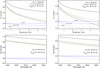Fig. 1 Estimation of the IQ at the focal plane of an 8m telescope as a function of the wavelength under a ε0 of 1.0 (left) and 0.7 (right) arcsec at 5000 Å, considering four different wavelength behaviors of the dome-turbulence (blue lines) contribution: (1) εdome=0 (solid green line), and (2, 3, and 4) εdome=0.2 arcsec at 5000 Å, with a power-law wavelength dependence of index γ=3 (2, dotted lines), γ=11/3 (3, dashed lines), and γ = 4 (4, dot-dashed lines). We assumed a typical ${ℒ}_0$ value of 22 m. The black solid curve follows the ε0 wavelength dependence (ε0 ∝ λ−1/5). The upper panels depict the general spectral range covered by instruments in ground-based optical-infrared observatories. The lower panels specifically showcase the spectral range of the MUSE integral field spectrograph, the selected instrument for implementing the proposed methodology on real data.

4 Application to real IFS observations

To apply the proposed methodology to actual data, we identified the MUSE instrument (Bacon et al. 2010) installed on the Nasmyth B platform of the European Southern Observatory (ESO) VLT Unit Four (UT4) at the Paranal Observatory⁵. MUSE is an integral field spectrograph providing spectral information in the range 4800–9300 Å with a mean resolution of 3000. In the seeing-limited mode (wide-field mode), MUSE samples a one-squared arcmin field of view with 0.2 arcsec spatial pixels. The VLT UT4 has a ~30m high dome, and the observing floor is ~10 m above ground level⁶. At about 100 m to the north of the UT4 building, a robotic DIMM monitors the turbulence conditions at Paranal on top of a 7m high tower (Sarazin 2017). Due to the difference in altitude between the DIMM tower and the Nasmyth VLT platform, we expect a slightly better ε₀ at the MUSE focal station (Δϵ_h), with a projected improvement of about Δϵ_h ~0.05 arcsec compared to the DIMM measurements (see Fig. 15 in Butterley et al. 2020), assuming a negligible dome turbulence contribution.

We used the extensive ESO science archive⁷ to collect the MUSE data. This archive offers thousands of reduced seeing-limited MUSE data cubes, ready for analysis. We note that any point-like source within the field of view of these data cubes can be a potential candidate for retrieving the prevailing atmospheric parameters during observations. To apply the method described in Sec. 3 to real data, we systematically searched the ESO science portal for processed data using the selection criteria outlined in Table 1 to constrain the number of potential data cubes to analyze. This search yielded a total of 718 data cubes, of which 389 were identified as being obtained in seeing-limited mode (labeled “WFM-NOAO” in the MUSE data cubes header). About 95.9% of them correspond to sky exposures, and 2.8% to unfocused calibration stars or extended objects, data cubes that are useless for the purpose of this work. Eventually, we concluded with five (1.3%) MUSE data cubes of two fields showing a few stars (see Fig. B.2). Table 2 presents the relevant parameters for the retrieved MUSE data cubes. Observations for the HD 90177 field (four data cubes) come from the same observing night, acquired within an interval of around two and a half hours (see Table 2).

We used the source detection tool within the photutils Astropy package⁸ to retrieve the positions of stars in the field of view of the selected MUSE data. For the subsequent analysis we focused on non-saturated bright stars isolated from companions within a radius of at least 5 arcsec. Then we used the MUSE Python Data Analysis Framework (MPDAF⁹; Piqueras et al. 2019) to recover band-filter images of an 8 arcsec² field of view centered on each selected star. For this, we designed a set of 100 Å wide bandpass filters uniformly distributed along the MUSE spectral axis, starting with the bluest at 4850 Å. The resulting 44 band-filter images for each star depict the seeing-limited MUSE PSF in the spectral coverage of those bands. We selected the analytical elliptical Moffat profile defined in Eq. (11) to model our band-filter images. We ensured a zero background in the Moffat profile by subtracting any sky background level from the band-filter images before performing the fitting: $$\text{ EM1 }=\frac{\text{ AM }}{{[1+A{(x-x_0)}^2+B{(y-y_0)}^2+C(x-x_0)(y-y_0)]}^{\beta }}\text{. }$$(11)

Here AM and β are the amplitude and the power index of the Moffat model centered on the star image peak at the field-of-view coordinates (x₀, y₀). The coefficients A, B, and C are defined as $$\begin{array}{rl}& A={\left(\frac{\cos \theta }{{\sigma }_1}\right)}^2+{\left(\frac{\sin \theta }{{\sigma }_2}\right)}^2;\\ & B={\left(\frac{\sin \theta }{{\sigma }_1}\right)}^2+{\left(\frac{\cos \theta }{{\sigma }_2}\right)}^2;\text{ and }\\ & C=2\sin \theta \cos \theta (\frac{1}{{\sigma }_1^2}-\frac{1}{{\sigma }_2^2}),\end{array}$$

where θ defines the orientation of the Moffat model with respect to the image axes, while σ₁ and σ₂ represent the characteristic widths of the profile along the major and minor axes, respectively, defining the ellipticity of the Moffat model. The Moffat function serves as a general model encompassing the Gaussian and Lorentzian functions, approaching each depending on the values of its parameters (e.g., Fétick et al. 2019; Trujillo et al. 2001). Specifically, for large values of β the Moffat function converges to a Gaussian profile, while for values close to unity it tends toward a Lorentzian profile.

We used a modified version of the Moffat2D model, incorporating an elliptical Moffat instead of a circular one. This model was introduced in the modeling module within the Astropy package, enabling the determination of the optimal parameters for fitting the Moffat model to the band-filter images recovered from MUSE data cubes. The FWHM of the PSF along the major and minor axes for each band-filter image is then determined from the Moffat parameters as follows: $${\mathrm{F}\mathrm{W}\mathrm{H}\mathrm{M}}_n=2\times {\sigma }_n\times \sqrt{2^{(1/\beta )}-1}\text{, with }n=1,2\text{. }$$(12)

Previous works, based on the analysis of stars, found that a circular Moffat profile with a power index of β ≈ 2.5 effectively reproduces the MUSE PSF across wavelengths (e.g., Bacon et al. 2015; Husser et al. 2016) in its seeing-limited mode. For other MUSE modes, including AO compensation, the PSF core is also approximated using a Moffat function (Fétick et al. 2019; Fusco et al. 2020).

We explored four distinct model configurations analyzing the residuals resulting from the subtraction of Moffat models from star images: (1) σ₁ = σ₂ and β as a free parameter; (2) σ₁ = σ₂ with a fixed β of 2.5; (3) both σ₁ and σ₂, as well as β as free parameters; and (4) σ₁ and σ₂ as free parameters with β fixed at 2.5 (see Esparza-Arredondo et al., in prep). Our findings show that residual levels remain comparable whether the β parameter is constrained to 2.5 or not. However, we obtained smaller residuals for an elliptical Moffat profile, even when σ₁ − σ₂ is significantly smaller than the spatial sampling. Subsequently, as a reference for analyzing the wavelength-dependent variation of MUSE IQ, we adopt the average FWHM derived from the σ_1,2 parameters obtained with configuration (4) of the Moffat model. Appendix B.2 presents the Moffat model parameters obtained for each individual star analyzed in this study.

Since the size and wavelength variation of IQ obtained from stars at distinct positions within the MUSE field of view are comparable within uncertainties, we computed the average IQ for each MUSE field (IQ_MUSE(λ), see Fig. 2) to compare it with the behavior predicted by Eq. (5). The standard deviation of these averaged IQ was taken as the uncertainty for IQ_MUSE (λ). From the ESO ambient conditions database for Paranal¹⁰, we retrieved the DIMM measurements recorded on the corresponding nights and computed the DIMM average value (ε_DIMM) during the MUSE observations (see Table 2). We estimated the natural ε₀ affecting the selected MUSE data cubes (ε_MUSE, listed in Table 3) by compensating for the expected improvement due to the DIMM-MUSE platform difference in height and projecting the result to the zenith angle (ζ) for the observations (Table 2): $${ϵ}_{\text{MUSE }}={\left(\frac{{\left[{ϵ}_{\text{DIMM }}\right]}^{5/3}-{\left[\mathrm{\Delta }{ϵ}_{\mathrm{h}}\right]}^{5/3}}{\cos \zeta }\right)}^{3/5}.$$(13)

For two of the five MUSE fields (HD 90177b and OGLEII), the measured IQ_MUSE consistently exceeds ε₀ at any wavelength (Fig. 2), while for the other three fields (HD 90177a, HD 90177c, and HD 90177d), the IQ is comparable or slightly lower across regions of the analyzed spectral range. This scenario is consistent with either an infinite ${ℒ}_0$ with some contribution from dome-induced turbulence or a finite ${ℒ}_0$ with a significant dome-induced blur. Previous works have reported a finite ${ℒ}_0$ at the Paranal Observatory, with a typical value of about 22 m (e.g., Ziad 2016), supporting the second as the most plausible option. Furthermore, the measured IQ_MUSE(λ) follows a similar curve to the predicted ε_LE through Eq. (5), although we observe some slope discrepancies for the analyzed fields. These discrepancies may suggest that the estimated ε_MUSE may not accurately represent the atmospheric turbulence affecting MUSE observations, indicating a non-negligible difference between the reported ε₀ by the DIMM and the actual ε₀ along the MUSE observation direction. Additionally, as discussed in Sec. 2, a nonnegligible ε_dome contribution may also contribute to these slope discrepancies.

Fortunately, the empirical IQ_MUSE measurements enable us to estimate the optimal combination of ε₀ and ${ℒ}_0$ values that best align with the observed data by fitting the analytical curve derived by Tokovinin (2002). Various fitting strategies may be employed for this purpose. However, the choice of a fitting method for implementing the proposed method to a specific instrument should be made after analyzing each particular case. The selected fitting method should align with the nature of the measurements, considering factors such as the number of empirical data points, sampling, spectral range, and uncertainties. It should also align with the intended use of the derived parameters. In this study we adopt a straightforward numerical approach, varying parameters to minimize residuals with the observed IQ_MUSE.

In particular, we used an iterative process involving variations in the input ε₀ within the analytical approach (i.e., Eq. (5)) across a range of possible values for the ε₀ along the MUSE observing direction. For our analysis, we explored ε₀ values from ε_MUSE − 0.2 to ε_MUSE + 0.5 arcsec, with 0.01 arcsec steps. For each specific ε₀ within this range, we determined the unknown parameter ${ℒ}_0$ by computing ${ℒ}_{0i}$ for each λ_i to match the measured IQ_MUSE(λ_i) and the predicted ε_LE(λ_i). The best-fit ${ℒ}_0$ value and its uncertainty were obtained as the average and standard deviation of these ${ℒ}_{0i}$ values. To account for the uncertainties in IQ_MUSE(λ_i), we performed a Monte Carlo (MC) simulation randomly varying IQ_MUSE(λ_i) within their uncertainty range many times (a thousand times for this work). The average and standard deviation of all these MC realizations were adopted as the observed ${ℒ}_0$ (${ℒ}_0^b$) and its uncertainty for that specific ε₀. After considering all combinations of ε₀ and ${ℒ}_0^b$, we adopted the best-fit parameters (i.e., ${ϵ}_0^b$ and ${ℒ}_0^b$) as those yielding the minimal residual with empirical IQ measurements.

Before analyzing the empirical measurement of IQ_MUSE to retrieve the combination of ε₀ and ${ℒ}_0$ that best matches the observations, we consider a potential blur contribution from turbulence inside the telescope dome or assume 100% atmospheric seeing-limited conditions, implying negligible dome-induced turbulence. We explore these two scenarios for the analyzed MUSE observed fields in the following subsections.

4.1 Analysis assuming negligible dome-induced turbulence

Under the assumption of a negligible dome turbulence contribution to the observed IQ, we wanted to determine the optimal combination of ε₀ and ${ℒ}_0$ predicting the best matching with the IQ_MUSE measurements. To achieve this, we used an iterative process involving variations of the input ε₀ within the Eq. (5) analytical approach, following the methodology described in the preceding section. Finally, we adopted the parameters providing minimal residuals between the predicted and measured IQ curves (${ϵ}_0^b$ and ${ℒ}_0^b$ in Fig. 2).

The derived ${ϵ}_0^b$ and ${ℒ}_0^b$ parameters (see Fig. 2 and Table 3) for the selected MUSE fields are consistent with the statistical distribution of these parameters at the Paranal Observatory (Ziad 2016; Otarola 2023).We found that the obtained ${ϵ}_0^b$ are on average 0.26 arcsec larger than those estimated from the DIMM measurements, with a minimum and maximum of 0.13 and 0.40 arcsec for HD 90177d and OGLEII fields, respectively. It is important to note that the MUSE observations were obtained at a higher airmass than typical for DIMM measurements. This, combined with the difference in observing directions between DIMM and MUSE, may contribute to these discrepancies. Interestingly, comparisons of ε₀ measurements from different atmospheric characterization instruments have found around 0.2 arcsec of discrepancy, attributed to the specific instrument locations on the Paranal Observatory plateau (e.g., Osborn et al. 2018). Consequently, the parameters obtained using the proposed methodology for the analyzed MUSE fields are compatible with purely seeing-limited observations, well within the statistical behavior of atmospheric turbulence at the Paranal Observatory.

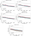Fig. 2 Wavelength dependence of IQ at the MUSE instrument’s focal plane (IQMUSE), analyzed using point-like sources in the MUSE fields indicated in each panel (see Table 2). The colored dots represent IQMUSE values derived from Moffat model fits for 44 band-filter images obtained from distinct stars within each MUSE field (individual plots available in Appendix B.2). The black open squares with error bars denote the average and standard deviation of the measured IQMUSE across all stars at each wavelength. The black dashed line shows the λ−1/5 behavior of the ε0 along the MUSE observation direction (εMUSE in arcseconds, top left corner), derived from average DIMM values during MUSE observations (see Table 2) using Eq. (13). The black solid and purple solid lines represent the ε0 and εLE that best fit the measurements obtained for the parameters ${ϵ}_0^b$ (in arcseconds) and ${ℒ}_0^b$ (in meters) in the bottom left corner of each plot (details in text).

4.2 Analysis assuming dome turbulence contribution

As discussed in Sec. 2, when the contribution of dome-induced turbulence becomes significant, it not only broadens the images, but can also influence the wavelength variation, depending on the nature of the dome’s local turbulence. In these cases, a direct measure of ε_dome at different wavelengths is desirable to properly isolate the broadening in the images due to the atmosphere and to apply the proposed methodology in this work to retrieve ${ℒ}_0$.

Unfortunately, we could not find a specific analysis of the ε_dome for the VLT UT4 telescope or any direct measurements of the dome contribution to turbulence degradation on the selected nights. However, Racine et al. (1991) found that the principal factors influencing the dome turbulence are the primary mirror and the enclosure temperatures, with contributions described as follows: $${ϵ}_{\mathrm{m}\mathrm{m}}\approx 0.4\times {(T_{\mathrm{m}\mathrm{m}}-T_{\mathrm{i}\mathrm{n}-\mathrm{e}\mathrm{n}})}^{6/5}\text{, and }$$(14) $${ϵ}_{\mathrm{e}\mathrm{n}}\approx 0.1\times {(T_{\text{in}-en}-T_{\text{out}-en})}^{6/5}\text{. }$$(15)

Here T_mm is the primary mirror temperature, and T_in–en and T_out–en are the temperatures inside and outside the telescope enclosure, respectively, assuming that T_in–en is the same at any location inside the dome. These contributions were empirically determined at an effective wavelength of 7000 Å (Racine et al. 1991). Hereafter, we assume that the Paranal VLT UT4 exhibits an equivalent behavior. Table 2 presents the recorded temperatures for the observation nights of the analyzed MUSE data cubes. Table 3 shows the estimates for dome-induced turbulence contribution during MUSE observations assuming Eqs. (14) and (15) apply to VLT UT4. On these nights the temperature of the main mirror of the telescope was lower than that inside the dome, preventing any turbulence from it, that is ε_mm = 0. However, the air within the dome was warmer than the outside environment, potentially leading to turbulence and contributing to the blur in the observed data. We adopted the estimated ε_en as the total ε_dome contribution to the measured IQ at a wavelength of 7000 Å (i.e., ε_dome(7000 Å) = ε_en).

Equation (8) allows us to extend the ε_dome approach from 7000 Å to any wavelength. Given the lack of a predefined power-law index γ, we treated it as a free parameter in the fitting procedure. As described in Sec. 4.1, we performed an iterative process involving the variations in the input ε₀ and the γ power-law index. Initially, we allowed ε₀ to vary within a range spanning from ε_MUSE − 0.2 to ε_MUSE + 0.5 arcsec, with steps of 0.01 arcsec. For each specific ε₀ value within this range, we followed these steps: (1) variations in the γ parameter in the range of 3 to 4, with steps of 0.01, to compute the dome turbulence contribution; (2) for each γ value, subtracting the resulting dome turbulence contribution from the measured IQ_MUSE(λ_i) at each wavelength to infer the ε_LE(λ_i) using Eq. (9); (3) determining the corresponding ${ℒ}_0$ from each ε_LE(λ_i), following the same methodology as described in previous sections. Subsequently, the combination of parameters (ε₀, λ, ${ℒ}_0$) yielding minimal residuals between the predicted (Eq. (5)) and measured IQ curves was adopted.

As in the previous section, we assess the uncertainties in the derived ε₀, γ, and ${ℒ}_0$ parameters using a MC approach. We randomly perturbed each IQ_MUSE(λ_i) within its uncertainty range for one thousand iterations, resulting in one thousand different sets of (ε₀, γ, ${ℒ}_0$) parameters. Finally, we calculated the average and standard deviation of these sets to determine the optimal combination that minimizes the residuals and provides the best fit to the observed data (see Table 3).

Figure 3 presents the results of this procedure applied to each of the selected MUSE data cubes. The obtained ${ϵ}_0^b$ and ${ℒ}_0^b$ parameters considering the dome turbulence contribution also align with the statistical distribution of these parameters at the Paranal Observatory (see Fig. 2 and Table 3). The differences between ${ϵ}_0^b$ and that expected from the DIMM measurements along the MUSE pointing are within the typical discrepancies of ε₀ measurements at different locations on the Paranal plateau (e.g., Osborn et al. 2018). We found some discrepancies in the estimated ${ℒ}_0^b$ for the four MUSE data cubes obtained on the same night in an interval of a few hours (see Table 2). Previous studies found significant variations in the ${ℒ}_0$ parameter on timescales comparable to fluctuations in other atmospheric parameters, such as ε₀ (e.g., Ziad 2016).

On the night with four data cubes of the same field (see Table 2), the analysis of the IQ_MUSE reveals dome-induced turbulence that varies with wavelength according to a power law, with an index larger than the Kolmogorov regime for three of them (i.e., HD 90177a, HD 90177c, and HD 90177d), while it is within the Kolmogorov regime for the HD 90177b data cube. The ε_dome parameters derived from these four MUSE data cubes indicate a subtle evolution of dome-induced turbulence throughout the night. This evolution primarily stems from changes in its power-law regime, while remaining nearly constant in terms of intensity at the reference wavelength (see Table 3). For the other field observed on a different night, the power-law index was smaller than the Kolmogorov $\gamma =\frac{11}{3}$ index.

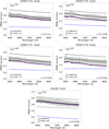Fig. 3 Same as Fig. 2, but considering the dome-turbulence contribution. The black open squares represent the average IQMUSE across each field, as in Fig. 2. The black filled squares show the IQ broadening attributed solely to atmospheric turbulence (i.e., IQMUSE after quadratically subtracting the estimated dome-turbulence contribution at each λ). The blue solid line corresponds to the estimated dome-turbulence contribution, following a power-law dependence on wavelength with the γ-index indicated in the bottom right corner. The green line corresponds to the quadratic sum of the predicted atmospheric (purple line) and dome (blue line) turbulence blur, fitting the measured MUSE IQ.

5 Conclusions

This work introduces a novel approach using IFS to measure the spatial coherence wavefront ${ℒ}_0$ prevailing during seeing-limited observations. This method takes advantage of the capability of IFS techniques to provide band-filter images over a wide wavelength range, all obtained under the same atmospheric and instrumental conditions. The homogeneity of IFS data enables the tracing of IQ variation with wavelength at the focal plane, directly linked to the prevailing ε₀ and ${ℒ}_0$ characterizing the atmospheric turbulence conditions. We applied the proposed technique to MUSE observations obtained at the Paranal Observatory, exploring two situations: one assuming negligible dome-induced turbulence and the other considering the ε_dome contribution. Through this analysis, the methodology accurately derived essential atmospheric parameters such as ε₀ and ${ℒ}_0$, while also revealing the wavelength dependence of the dome-induced turbulence, providing valuable insights into atmospheric conditions and instrument performance. The main findings and conclusions of this work can be summarized as follows:

• IFS is a powerful tool for astronomical observations, enabling simultaneous spatial and spectral datasets over wide fields and wavelength ranges;

• The homogeneity of the data cubes resulting from IFS observations provides a collection of band-filter images that allow for comprehensive analysis of IQ variations with wavelength. The S/N of each band-filter image is crucial for precise IQ assessment;

• IFS enables the empirical verification of the analytical approximation to IQ variations with wavelength (Eqs. (5) and (6)), derived from simplified models of atmospheric turbulence theory. We accomplished this validation using IFS data obtained with the MUSE instrument at the Paranal Observatory;

• The MUSE PSF is well described by a Moffat Model with the power-law index set to a value of 2.5 at any wavelength. We adopt the Moffat model FWHM as the metric for assessing the MUSE IQ;

• In both dome-seeing scenarios considered, assuming a negligible or non-negligible ε_dome, the derived ${ϵ}_0^b$ and ${ℒ}_0^b$ parameters for the analyzed MUSE fields align with the statistical behavior of these parameters at the Paranal Observatory, supporting that MUSE provides predominantly seeing-limited observations. Moreover, the differences between the retrieved ${ϵ}_0^b$ and the MUSE seeing estimated from DIMM are within the typical discrepancies of ε₀ measurements at various locations on the Paranal plateau found with different instruments;

• Direct measurements of ε_dome at various wavelengths are crucial for accurately isolating atmospheric broadening and determining ${ℒ}_0$.

Seeing-limited integral field spectrographs commonly operate in ground-based observatories. As a by-product of these observations, the ${ℒ}_0$ parameter could be routinely obtained and also facilitate the tracking of dome-induced turbulence. A reassessment of observing strategies for IFS observations, especially during the observation of calibration stars, may be beneficial to implement the proposed methodology for site characterization purposes.

Acknowledgements

Based on data obtained from the ESO science archive facility with DOI(s): https://doi.eso.org/10.18727/archive/41. The authors acknowledge support from the Spanish Ministry of Science and Innovation through the Spanish State Research Agency (AEI-MCINN/10.13039/501100011033) through grants “Participation of the Instituto de Astrofísica de Canarias in the development of HARMONI: D1 and Delta-D1 phases” with references PID2019-107010GB-100 and PID2022-140483NB-C21 and the Severo Ochoa Program 2020–2023 (CEX2019-000920-S).

Appendix A Comparison of the two analytical functions approaching the image quality

We computed the predicted IQ as a function of wavelength considering various telescope diameters and turbulence conditions (Fig. A.1) using Eqs. 5 and 6, and tracking the atmospheric conditions where ${ℒ}_0$/r₀ > 20. Figure A.1 shows that the two equations provide similar assessments for the IQ at the focal plane of telescopes. The differences become more notable for decreasing telescope diameter and increasing size of the ${ℒ}_0$ parameter of the turbulence. As a general trend, it is important to note that these approaches apply only to wavelengths within the range of 3700 to 9300 Å for ${ℒ}_0$ ≤ 12 m and excellent ε₀ conditions, to maintain relative error within ±1%. For typical ε₀ (e.g., Skidmore et al. 2009; Vázquez Ramió et al. 2012) and ${ℒ}_0$ (e.g., Ziad 2016) at astronomical sites, the applicability without exceeding the ±1% error extends up to 15000 Å.

In the case of poor atmospheric turbulence conditions, these approaches are usable with ±1% uncertainty up to 3 μm. Figure A.2 shows a zoomed-in image of the predicted IQ(λ) for the spectral range of the MUSE instrument, whose data are used in this work to illustrate the applicability of the proposed method for estimating the ${ℒ}_0$ of turbulence from IFS observations.

Figure A.3 shows the wavelength average ratio of ε_LE(λ) and ε_LE(λ, $\mathcal{D}$) as a function of the ${ℒ}_0$ for different ε₀ conditions and telescope diameters. The diameter becomes relevant for small telescopes (i.e., $\mathcal{D}$ < 1.5 m), underestimating the image quality by more than ~2%, ~4%, and ~6% in the optical (i.e., 3700–9300 Å), 0.93–2.5 μm, and 2.5–5 μm spectral ranges, respectively. For medium to large telescopes (4m to 10m class telescopes), the image quality is underestimated by a factor always < 5% in the entire near-infrared range (i.e., 0.93–5 μm), being <2% at the optical for any turbulence condition. For extremely large telescopes (i.e., $\mathcal{D}$ > ~20 m), the ε_LE(λ)/ε_LE(λ, $\mathcal{D}$) is always almost 1.

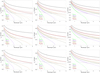Fig. A.1 Predicted image quality for a long-exposure image (e.g., λLE) of a point-like source obtained using ground-based telescopes with diameters of 1.5 m (top), 8 m (middle), and 39 m (bottom), as a function of the wavelength. The panels correspond to different λ0 conditions at 5000 Å: 0.4 arcsec (left panels), 0.7 arcsec (central panels), and 1.5 arcsec (right panels). Each curve corresponds to the indicated value of the ${ℒ}_0$ of the turbulence in meters: ${ℒ}_0$=100 → red, ${ℒ}_0$=32→ orange, ${ℒ}_0$=22 → olive green, ${ℒ}_0$=12 → purple, and ${ℒ}_0$=5 → lime green. The black curve follows the ε0 wavelength dependence (ε0(λ) ∝ λ−1/5), corresponding to ${ℒ}_0$=∞. The solid curves correspond to the first-order approach to εLE following Eq. 5, while the dashed curves to the second-order approach considering the telescope diameter (Eq. 6). The dotted line delineates the ${ℒ}_0$/r0>20 boundary, above which errors are constrained within ±1%.

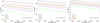Fig. A.2 Same as Fig. A.1, but for the parameters of the MUSE instrument, the IFS installed at the 8m VLT operating in the optical range between 4750 and 9350 Å.

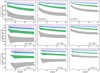Fig. A.3 Wavelength average ratio of the two approaches for estimating the image quality at the focal plane of a telescope (i.e., εLE(λ)/εLE(λ, $\mathcal{D}$ from Eqs. 5 and 6) as a function of the ${ℒ}_0$ of the turbulence for the spectral ranges 3700–9300 Å (top panels); 0.93–2.5 μm (middle panels); and 2.5–5.0 μm (bottom panels) at excellent (left panels), typical (central panels), and fair (right panels) atmosheric turbulence conditions. We considered only those conditions with ${ℒ}_0$/r0>20, ensuring that errors are within ±1%. The shaded area marks the 1σ of the mean. The colors indicate different telescope diameters as indicated at the right side of each panel.

Appendix B Band-filter images recovered from IFS data

In this appendix we use a simple model to analyze the putative impact of the band-filter width selected to recover band-filter images from IFS data cubes on the expected IQ of the image. We also include the parameters derived for the Moffat profile fits to model the IQ of band-filter images recovered from MUSE observations.

B.1 Impact of the band-filter width

We performed a simple simulation of seeing-limited IFS observations in the optical range spanning from 3500 to 7500 Å for two point-like sources to explore the effect of bandwidth on the measured IQ. We chose the spectra of HD000319 (type A1V) and HD001326B (type M6 V) stars (see Fig. B.1) from the MILES stellar library (Sánchez-Blázquez et al. 2006). We selected two stars with different spectral emissions to also assess the influence of the source spectral behavior on the IQ measurements from band-filter images.

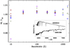Fig. B.1 IQ of band-filter images recovered from mock IFS observations of the stars in the inset plot, relative to the input εLE for the simulation, plotted as a function of the bandwidths used for image recovery. Turbulence conditions were set to ε0=0.83 arcsec and ${ℒ}_0$=22 m to compute εLE from Eq. 5. Filled and open circles correspond to mock IFS observations of the A1V-type (HD000136) and M6 V-type (HD001326) stars, respectively. The colors correspond to the central wavelength of the band filters: ε1 = 4000Å → purple, λ2 = 5000Å → blue, λ3 = 6000Å → green, and λ4 = 7000Å → red.

We generated a mock data cube for a 1′ × 1′ field of view, using spaxels with dimensions (Δα, Δδ, Δλ)=(0.″1,0.″ 1, 1Å). We modeled the seeing-limited PSF using a circular Gaussian distribution, with the FWHM varying with wavelength in accordance with the predicted ε_LE(λ) derived from Eq. 5 for a ε₀ and ${ℒ}_0$ of 0.83 arcsec and 22 m, respectively (Martinez et al. 2010), typical values at the Paranal Observatory. Each wavelength slice was perturbed by normally distributed pseudo-random noise with a mean of zero and a standard deviation of one, ensuring a minimum S/N of 5 per slice.

From the mock data cubes, we chose four central wavelengths (λ₁ = 4000, λ₂ = 5000, λ₃ = 6000, and λ₄ = 7000 Å) to recover five band-filter images at each wavelength, using bandwidths of 10, 30, 100, 250, and 500 Å. Additionally, we recovered broadband filter images with widths of 1000 and 1500 Å, centered on λ₂ and λ₃.

Figure B.1 presents a comparison between the expected ε_LE at λ_i and the measured FWHMλ_i of recovered filter images within the spectral bands $[{\lambda }_i-\frac{N}{2},{\lambda }_i+\frac{N}{2}]$, with i=1,2,3,4, and N=30,100,250,500, and N=1000, 1500 for i=2,3. We selected Δλ=1 Å in the mock data cube to simplify the assessment. The resulting IQ varies less than ±1% with respect to the input ε_LE(λ_i) of the slice at λ_i corresponding to the central wavelength of the bands in almost all the recovered images.

For the 10 Å bandwidth filter images, the S/N strongly contributes to the discrepancies between IQ and ε_LE. A minimum S/N of 25 seems to be an adequate threshold for the measurement of the image PSF widths. The spectral energy distribution of the observed object also impacts the outcomes, with more notable deviations occurring when the central wavelength of the band filter coincides with a spectral region of weak emission in the source. Therefore, in general, deviations tend to increase with wider bands, although the S/N of recovered band-filter images and the spectrum of the observed object could also contribute to these deviations. Henceforth, for band-filter images obtained from seeing-limited IFS observations with S/N≥25, we assume uncertainties less than 1% of the PSF FWHM, specifically associated with the chosen filter bandwidths for image recovery.

B.2 Parameters of the Moffat models fitted to band-filter images of isolated stars in MUSE data cubes

We present here the images of the MUSE observed fields identifying the stars analyzed in this study to trace image quality across wavelengths (see Fig. B.2). We also present the wavelength variation of the centroids and widths (i.e., x₀, y₀, σ₁, and σ₂ parameters in section 3) for the Moffat fitting profiles models to the 44 narrowband filter images recovered for each selected star for each observed field within the MUSE retrieved data cubes. Differences in FWHMs derived from the σ_i (i=1,2) parameters along the two axes are almost always smaller than the MUSE spatial sampling (i.e., 0.2 arcsec). Therefore, we define the IQ(λ_i) as the average of the FWHM₁ and FWHM₂ at each λ_i. Following the same approach as outlined in section 4.1, we determine a combination of ${ϵ}_0^b$ and ${ℒ}_0^b$ values that best fit the IQ(λ) for each of the stars analyzed in each MUSE field. We provide a case-by-case description of the MUSE fields, Moffat fittings, and the optimal ${ϵ}_0^b$ and ${ℒ}_0^b$ combinations that match the measured IQ(λ_i) for each star in Table B.1, which summarizes the results. The dispersion of the derived atmospheric parameters from individual stars in the same field provides the typical error of the proposed methodology.

B.2.1 HD90177 field

HD90177 is a luminous blue variable star in the Carina Nebula, one of the largest diffuse nebulae in the southern sky, hosting numerous massive and young stars. HD90177 is known for intense mass-loss episodes, and it is surrounded by a unique stellar population distribution suggesting a potential association with a moving group of B-type stars in a spiral arm (Mehner et al. 2021).

We obtained four MUSE data cubes labeled HD90177a, HD90177b, HD90177c, and HD90177d (see Table 2) for the D90177 field. All were observed on the same night within a temporal window of just under three hours. The star HD90177, located at the center of the MUSE data cubes, generates strong stray light artifacts due to its brightness that affect some stars in the observed MUSE field, which includes many other fainter stars than HD90177 (Fig. B.2, left). We identified 14 stars in the field without detected companions within a circular aperture of 5 arcsec radius. Among them, we discarded four stars due to contamination by stray light from the central bright star. Additionally, five stars had low S/N in at least 50% of the defined filter bands in any of the four MUSE data cubes, and one star was too close to the field border, which prevented a proper fitting of the Moffat model. Figures B.3, B.4, B.5, and B.6 present the parameters for the Moffat model profiles fitted to the band-filter images of the remaining four stars in this field for the four MUSE data cubes, plotted against the central wavelengths of the respective bands.

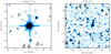Fig. B.2 Broadband filter images recovered from MUSE observations of the fields HD90177 (left) and OGLEII (right).

The centroids of the Moffat models follow wavelength-dependent variations, which are different for each star but consistently within ±0.2 arcsec, corresponding to one MUSE spatial pixel. The σ_i (i=1,2) parameters for the Moffat models decrease for increasing wavelengths similarly for the four stars.

The values for ${ϵ}_0^b$ derived from the analysis of the IQ for each star in the four MUSE data cubes for the HD90177 field are compatible, with an average and standard deviation of 0.79 ± 0.02, 0.76 ± 0.03, 0.81 ± 0.02, and 0.70 ± 0.06 arcsec for the HD90177a, HD90177b, HD90177c, and HD90177d data cubes, respectively (see Table B.1). The average and standard deviation of the ${ℒ}_0^b$ values derived from each star are 21.12 ± 5.83, 23.20 ± 8.69, 16.77 ± 2.16, and 30.80 ± 12.66 meters, respectively, for the HD90177a, HD90177b, HD90177c, and HD90177d data cubes.

B.2.2 OGLEII

The MUSE field labeled “OGLEII” seems to correspond to an observation of the “OGLEII dia bul-sc01 1821” star, according to the MUSE data cube header. This star is a Mira variable that is included in the X-Shooter spectral library (Gonneau et al. 2020). Located in the galactic bulge region, the MUSE data cube shows a high density of stars of different brightness (Fig. B.2, right). We found ten stars in the MUSE field without companions brighter than a 5σ background within a region of 5 arcsec radius. Among them, we excluded three stars because the surrounding background revealed the presence of faint stars, impacting the fitting of the Moffat model. Additionally, we discarded one star due to a poor S/N in at least 50% of the defined filter bands. In Fig. B.11 we show the parameters against the central wavelengths of the respective filter for the Moffat model profiles fitted to the band-filter images of the remaining six stars. We observe wavelength-dependent variations in the centroids within the ±0.2 arcsec of the MUSE spatial pixel for most of the measurements, with the largest deviations along the horizontal axis. As expected, the Moffat model’s widths decrease as wavelengths increase. For the analyzed stars in this field, Star-7 displays the most significant deviation from a circular Moffat model on average. The values for ${ϵ}_0^b$ derived from the analysis of the IQ for each star in the OGLEII field are compatible, with an average and standard deviation of 0.94 ± 0.05 arcsec (see Table B.1). The average and standard deviation of the ${ℒ}_0^b$ values derived from each star are 16.3 ± 7.6 m.

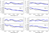Fig. B.3 Characteristic parameters of the Moffat profile model with β = 2.5 fitting the 44 narrowband filter images of selected point-like sources in the MUSE Field of HD90177 labeled HD90177a (see Fig. B.2, top left). The top panels show the wavelength-dependent variations of the centroid (x0,y0) with respect to the average star peak location (indicated by the dashed horizontal line). The bottom panels present the variation in the width parameter σi (i=1,2) with wavelength. Measurements along axis i=1 (horizontal) and i=2 (vertical) are represented by filled black circles and blue squares, respectively. The star numbers correspond to the star labels in Fig. B.2 (top left).

Fig. B.4 Same as Fig. B.3, but for the MUSE data cube labeled HD90177b.

Fig. B.5 Same as Fig. B.3, but for the MUSE data cube labeled HD90177c.

Fig. B.6 Same as Fig. B.3, but for the MUSE data cube labeled HD90177d.

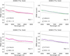Fig. B.7 Wavelength variation in the average FWHM for the Moffat fitting profile to the narrowband filter images recovered for each of the selected stars in the MUSE HD90177 field labeled HD90177a (see Fig. B.2, left). The dashed black curve corresponds to the wavelength behavior of the ε0 derived from the average DIMM values during the MUSE observations (see Table 1). The combination of ε0 and ${ℒ}_0$ best fitting the observations is indicated in the left corner of each panel; the values were obtained by minimizing the residuals, while varying ε0 and ${ℒ}_0$ values. The purple line corresponds to the wavelength εLE variation using ${ϵ}_0^b$ and ${ℒ}_0$b. The black solid line represents the λ−1/5 behaviour using ${ϵ}_0^b$.

Fig. B.8 Same as Fig. B.7, but for the MUSE data cube labeled HD90177b.

Fig. B.9 Same as Fig. B.9, but for the MUSE data cube labeled HD90177c.

Fig. B.10 Same as Fig. B.10, but for the MUSE data cube labeled HD90177d.

Fig. B.11 Same as Fig. B.3, but for the MUSE data cube of the OGLEII field.

Fig. B.12 Same as Fig. B.7, but for the MUSE data cube of the OGLEII field.

References

All Tables

All Figures

Fig. 1 Estimation of the IQ at the focal plane of an 8m telescope as a function of the wavelength under a ε0 of 1.0 (left) and 0.7 (right) arcsec at 5000 Å, considering four different wavelength behaviors of the dome-turbulence (blue lines) contribution: (1) εdome=0 (solid green line), and (2, 3, and 4) εdome=0.2 arcsec at 5000 Å, with a power-law wavelength dependence of index γ=3 (2, dotted lines), γ=11/3 (3, dashed lines), and γ = 4 (4, dot-dashed lines). We assumed a typical ${ℒ}_0$ value of 22 m. The black solid curve follows the ε0 wavelength dependence (ε0 ∝ λ−1/5). The upper panels depict the general spectral range covered by instruments in ground-based optical-infrared observatories. The lower panels specifically showcase the spectral range of the MUSE integral field spectrograph, the selected instrument for implementing the proposed methodology on real data.

In the text

Fig. 2 Wavelength dependence of IQ at the MUSE instrument’s focal plane (IQMUSE), analyzed using point-like sources in the MUSE fields indicated in each panel (see Table 2). The colored dots represent IQMUSE values derived from Moffat model fits for 44 band-filter images obtained from distinct stars within each MUSE field (individual plots available in Appendix B.2). The black open squares with error bars denote the average and standard deviation of the measured IQMUSE across all stars at each wavelength. The black dashed line shows the λ−1/5 behavior of the ε0 along the MUSE observation direction (εMUSE in arcseconds, top left corner), derived from average DIMM values during MUSE observations (see Table 2) using Eq. (13). The black solid and purple solid lines represent the ε0 and εLE that best fit the measurements obtained for the parameters ${ϵ}_0^b$ (in arcseconds) and ${ℒ}_0^b$ (in meters) in the bottom left corner of each plot (details in text).

In the text

Fig. 3 Same as Fig. 2, but considering the dome-turbulence contribution. The black open squares represent the average IQMUSE across each field, as in Fig. 2. The black filled squares show the IQ broadening attributed solely to atmospheric turbulence (i.e., IQMUSE after quadratically subtracting the estimated dome-turbulence contribution at each λ). The blue solid line corresponds to the estimated dome-turbulence contribution, following a power-law dependence on wavelength with the γ-index indicated in the bottom right corner. The green line corresponds to the quadratic sum of the predicted atmospheric (purple line) and dome (blue line) turbulence blur, fitting the measured MUSE IQ.

In the text

Fig. A.1 Predicted image quality for a long-exposure image (e.g., λLE) of a point-like source obtained using ground-based telescopes with diameters of 1.5 m (top), 8 m (middle), and 39 m (bottom), as a function of the wavelength. The panels correspond to different λ0 conditions at 5000 Å: 0.4 arcsec (left panels), 0.7 arcsec (central panels), and 1.5 arcsec (right panels). Each curve corresponds to the indicated value of the ${ℒ}_0$ of the turbulence in meters: ${ℒ}_0$=100 → red, ${ℒ}_0$=32→ orange, ${ℒ}_0$=22 → olive green, ${ℒ}_0$=12 → purple, and ${ℒ}_0$=5 → lime green. The black curve follows the ε0 wavelength dependence (ε0(λ) ∝ λ−1/5), corresponding to ${ℒ}_0$=∞. The solid curves correspond to the first-order approach to εLE following Eq. 5, while the dashed curves to the second-order approach considering the telescope diameter (Eq. 6). The dotted line delineates the ${ℒ}_0$/r0>20 boundary, above which errors are constrained within ±1%.

In the text

	Fig. A.2 Same as Fig. A.1, but for the parameters of the MUSE instrument, the IFS installed at the 8m VLT operating in the optical range between 4750 and 9350 Å.
In the text

Fig. A.3 Wavelength average ratio of the two approaches for estimating the image quality at the focal plane of a telescope (i.e., εLE(λ)/εLE(λ, $\mathcal{D}$ from Eqs. 5 and 6) as a function of the ${ℒ}_0$ of the turbulence for the spectral ranges 3700–9300 Å (top panels); 0.93–2.5 μm (middle panels); and 2.5–5.0 μm (bottom panels) at excellent (left panels), typical (central panels), and fair (right panels) atmosheric turbulence conditions. We considered only those conditions with ${ℒ}_0$/r0>20, ensuring that errors are within ±1%. The shaded area marks the 1σ of the mean. The colors indicate different telescope diameters as indicated at the right side of each panel.

In the text

Fig. B.1 IQ of band-filter images recovered from mock IFS observations of the stars in the inset plot, relative to the input εLE for the simulation, plotted as a function of the bandwidths used for image recovery. Turbulence conditions were set to ε0=0.83 arcsec and ${ℒ}_0$=22 m to compute εLE from Eq. 5. Filled and open circles correspond to mock IFS observations of the A1V-type (HD000136) and M6 V-type (HD001326) stars, respectively. The colors correspond to the central wavelength of the band filters: ε1 = 4000Å → purple, λ2 = 5000Å → blue, λ3 = 6000Å → green, and λ4 = 7000Å → red.

In the text

	Fig. B.2 Broadband filter images recovered from MUSE observations of the fields HD90177 (left) and OGLEII (right).
In the text

Fig. B.3 Characteristic parameters of the Moffat profile model with β = 2.5 fitting the 44 narrowband filter images of selected point-like sources in the MUSE Field of HD90177 labeled HD90177a (see Fig. B.2, top left). The top panels show the wavelength-dependent variations of the centroid (x0,y0) with respect to the average star peak location (indicated by the dashed horizontal line). The bottom panels present the variation in the width parameter σi (i=1,2) with wavelength. Measurements along axis i=1 (horizontal) and i=2 (vertical) are represented by filled black circles and blue squares, respectively. The star numbers correspond to the star labels in Fig. B.2 (top left).

In the text

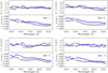	Fig. B.4 Same as Fig. B.3, but for the MUSE data cube labeled HD90177b.
In the text

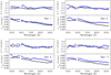	Fig. B.5 Same as Fig. B.3, but for the MUSE data cube labeled HD90177c.
In the text

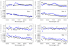	Fig. B.6 Same as Fig. B.3, but for the MUSE data cube labeled HD90177d.
In the text

Fig. B.7 Wavelength variation in the average FWHM for the Moffat fitting profile to the narrowband filter images recovered for each of the selected stars in the MUSE HD90177 field labeled HD90177a (see Fig. B.2, left). The dashed black curve corresponds to the wavelength behavior of the ε0 derived from the average DIMM values during the MUSE observations (see Table 1). The combination of ε0 and ${ℒ}_0$ best fitting the observations is indicated in the left corner of each panel; the values were obtained by minimizing the residuals, while varying ε0 and ${ℒ}_0$ values. The purple line corresponds to the wavelength εLE variation using ${ϵ}_0^b$ and ${ℒ}_0$b. The black solid line represents the λ−1/5 behaviour using ${ϵ}_0^b$.

In the text

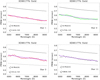	Fig. B.8 Same as Fig. B.7, but for the MUSE data cube labeled HD90177b.
In the text

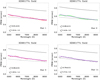	Fig. B.9 Same as Fig. B.9, but for the MUSE data cube labeled HD90177c.
In the text

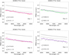	Fig. B.10 Same as Fig. B.10, but for the MUSE data cube labeled HD90177d.
In the text

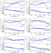	Fig. B.11 Same as Fig. B.3, but for the MUSE data cube of the OGLEII field.
In the text

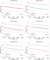	Fig. B.12 Same as Fig. B.7, but for the MUSE data cube of the OGLEII field.
In the text

References

- Abahamid, A., Jabiri, A., Vernin, J., et al. 2004, A&A, 416, 1193 [NASA ADS] [CrossRef] [EDP Sciences] [Google Scholar]
- Allington-Smith, J. 2006, New Astron. Rev., 50, 244 [CrossRef] [Google Scholar]
- Bacon, R., Accardo, M., Adjali, L., et al. 2010, SPIE Conf. Ser., 7735, 773508 [Google Scholar]
- Bacon, R., Brinchmann, J., Richard, J., et al. 2015, A&A, 575, A75 [NASA ADS] [CrossRef] [EDP Sciences] [Google Scholar]
- Borgnino, J. 1990, Appl. Opt., 29, 1863 [CrossRef] [Google Scholar]
- Bustos, E., & Tokovinin, A. 2018, SPIE Conf. Ser., 10700, 107000Q [NASA ADS] [Google Scholar]
- Butterley, T., Wilson, R. W., Sarazin, M., et al. 2020, MNRAS, 492, 934 [NASA ADS] [CrossRef] [Google Scholar]
- Fétick, R. J. L., Fusco, T., Neichel, B., et al. 2019, A&A, 628, A99 [NASA ADS] [CrossRef] [EDP Sciences] [Google Scholar]
- Floyd, D. J. E., Thomas-Osip, J., & Prieto, G. 2010, PASP, 122, 731 [CrossRef] [Google Scholar]
- Fried, D. L. 1965, J. Opt. Soc. Am., 55, 1427 [NASA ADS] [CrossRef] [Google Scholar]
- Fusco, T., Bacon, R., Kamann, S., et al. 2020, A&A, 635, A208 [NASA ADS] [CrossRef] [EDP Sciences] [Google Scholar]
- García-Lorenzo, B., Esparza-Arredondo, D., Acosta-Pulido, J. A., & Castro-Almazán, J. A. 2023, in COAT2023: Communications and Observations through Atmospheric Turbulence, https://jamesosborn.webspace.durham.ac.uk/coat-2023/ [Google Scholar]
- Gonneau, A., Lyubenova, M., Lançon, A., et al. 2020, A&A, 634, A133 [NASA ADS] [CrossRef] [EDP Sciences] [Google Scholar]
- Guesalaga, A., Neichel, B., Correia, C. M., et al. 2017, MNRAS, 465, 1984 [NASA ADS] [CrossRef] [Google Scholar]
- Harrison, C. M. 2016, Integral Field Spectroscopy and Spectral Energy Distributions (Cham: Springer International Publishing), 37 [Google Scholar]
- Henry, J. P., Heyer, I., Cecil, G., Barnes, B., & Cheigh, F. 1987, PASP, 99, 1354 [NASA ADS] [CrossRef] [Google Scholar]
- Husemann, B., Bennert, V. N., Scharwächter, J., Woo, J.-H., & Choudhury, O. S. 2016, MNRAS, 455, 1905 [NASA ADS] [CrossRef] [Google Scholar]
- Husser, T.-O., Kamann, S., Dreizler, S., et al. 2016, A&A, 588, A148 [NASA ADS] [CrossRef] [EDP Sciences] [Google Scholar]
- Lai, O., Withington, J. K., Laugier, R., & Chun, M. 2019, MNRAS, 484, 5568 [Google Scholar]
- Martinez, P., Kolb, J., Tokovinin, A., & Sarazin, M. 2010, A&A, 516, A90 [NASA ADS] [CrossRef] [EDP Sciences] [Google Scholar]
- Mehner, A., Janssens, S., Agliozzo, C., et al. 2021, A&A, 655, A33 [NASA ADS] [CrossRef] [EDP Sciences] [Google Scholar]
- Munro, J., Hansen, J., Travouillon, T., Grosse, D., & Tokovinin, A. 2023, J. Astron. Telescopes Instrum. Syst., 9, 017004 [NASA ADS] [Google Scholar]
- Osborn, J., & Alaluf, D. 2023, MNRAS, 525, 1936 [NASA ADS] [CrossRef] [Google Scholar]
- Osborn, J., Wilson, R. W., Sarazin, M., et al. 2018, MNRAS, 478, 825 [CrossRef] [Google Scholar]
- Otarola, A. 2023, in COAT2023: Communications and Observations through Atmospheric Turbulence, https://jamesosborn.webspace.durham.ac.uk/coat-2023/ [Google Scholar]
- Piqueras, L., Conseil, S., Shepherd, M., et al. 2019, in ASP Conf. Ser., 521, Astronomical Data Analysis Software and Systems XXVI, eds. M. Molinaro, K. Shortridge, & F. Pasian, 545 [Google Scholar]
- Racine, R., Salmon, D., Cowley, D., & Sovka, J. 1991, PASP, 103, 1020 [NASA ADS] [CrossRef] [Google Scholar]
- Roddier, F. 1981, Prog. Opt., 19, 281 [Google Scholar]
- Sánchez-Blázquez, P., Peletier, R. F., Jiménez-Vicente, J., et al. 2006, MNRAS, 371, 703 [Google Scholar]
- Sarazin, M. 2017, Astronomical Site Monitor Data User Manual (ESO-281474), ESO-281474, 29 [Google Scholar]
- Sarazin, M., & Roddier, F. 1990, A&A, 227, 294 [NASA ADS] [Google Scholar]
- Skidmore, W., Els, S., Travouillon, T., et al. 2009, PASP, 121, 1151 [NASA ADS] [CrossRef] [Google Scholar]
- Stubbs, C. W. 2021, MNRAS, 508, 3936 [NASA ADS] [CrossRef] [Google Scholar]
- Tokovinin, A. 2002, PASP, 114, 1156 [CrossRef] [Google Scholar]
- Tokovinin, A., Sarazin, M., & Smette, A. 2007, MNRAS, 378, 701 [CrossRef] [Google Scholar]
- Toselli, I., Andrews, L. C., Phillips, R. L., & Ferrero, V. 2007, SPIE Conf. Ser., 6551, 65510E [Google Scholar]
- Trujillo, I., Aguerri, J. A. L., Cepa, J., & Gutiérrez, C. M. 2001, MNRAS, 328, 977 [NASA ADS] [CrossRef] [Google Scholar]
- Vázquez Ramió, H., Vernin, J., Muñoz-Tuñón, C., et al. 2012, PASP, 124, 868 [CrossRef] [Google Scholar]
- Voitsekhovich, V. V. 1995, J. Opt. Soc. Am. A, 12, 1346 [NASA ADS] [CrossRef] [Google Scholar]
- Winker, D. M. 1991, J. Opt. Soc. Am. A, 8, 1568 [CrossRef] [Google Scholar]
- Woolf, N. 1979, PASP, 91, 523 [CrossRef] [Google Scholar]
- Ziad, A. 2016, SPIE Conf. Ser., 9909, 99091K [NASA ADS] [Google Scholar]
- Ziad, A., Conan, R., Tokovinin, A., Martin, F., & Borgnino, J. 2000, Appl. Opt., 39, 5415 [NASA ADS] [CrossRef] [Google Scholar]
All Tables
Selection criteria used in the ESO Science Portal for identifying processed data cubes from IFS observations.
Parameter for the MUSE processed data cubes downloaded from the ESO Science Portal.
Atmospheric parameters derived from the measured IQ at different wavelengths from MUSE data cubes.
Atmospheric parameters derived from the measured image quality at different wavelengths from MUSE data cubes.