| Issue |
A&A
Volume 686, June 2024
|
|
|---|---|---|
| Article Number | A19 | |
| Number of page(s) | 26 | |
| Section | Planets and planetary systems | |
| DOI | https://doi.org/10.1051/0004-6361/202449233 | |
| Published online | 24 May 2024 | |
Search for giant planets in M 67 V: A warm Jupiter orbiting the turn-off star S1429
1
Universitäts-Sternwarte München, Fakultät für Physik, Ludwig-Maximilians-Universität München,
Scheinerstr. 1,
81679
München,
Germany
e-mail: This email address is being protected from spambots. You need JavaScript enabled to view it.
2
Max-Planck-Institut für extraterrestrische Physik,
Giessenbachstrasse 1,
85748
Garching,
Germany
3
ESO-European Southern Observatory,
Karl-Schwarzschild-Strasse 2,
85748
Garching bei München,
Germany
4
Istituto Nazionale di Astrofisica, Osservatorio Astrofisico di Arcetri,
50125
Firenze,
Italy
5
GEPI, Observatoire de Paris, Université PSL, CNRS,
5 Place Jules Janssen,
92190
Meudon,
France
6
Departamento de Física Teórica e Experimental, Universidade Federal do Rio Grande do Norte, Campus Universitário,
Natal, RN,
59072-970,
Brazil
7
Georg-August-Universität, Institut für Astrophysik und Geophysik,
Friedrich-Hund-Platz 1,
37077
Göttingen,
Germany
8
Instituto Nazionale di Astrofisica, Osservatorio Astronomico di Padova,
35122
Padova,
Italy
9
Instituto Nazionale di Astrofisica, Osservatorio Astronomico di Roma,
via Frascati 33,
Monte Porzio Catone,
Italy
Received:
15
January
2024
Accepted:
28
February
2024
Abstract
Context. Planets orbiting members of open or globular clusters offer a great opportunity to study exoplanet populations systematically, as stars within clusters provide a mostly homogeneous sample, at least in chemical composition and stellar age. However, even though there have been coordinated efforts to search for exoplanets in stellar clusters, only a small number of planets have been detected. One successful example is the seven-year radial velocity (RV) survey ‘Search for giant planets in M 67’ of 88 stars in the open cluster M 67, which led to the discovery of five giant planets, including three close-in (P < 10 days) hot-Jupiters.
Aims. In this work, we continue and extend the observation of stars in M 67, with the aim being to search for additional planets.
Methods. We conducted spectroscopic observations with the Habitable Planet Finder (HPF), HARPS, HARPS-North, and SOPHIE spectrographs of 11 stars in M 67. Six of our targets showed a variation or long-term trends in their RV during the original survey, while the other five were not observed in the original sample, bringing the total number of stars to 93.
Results. An analysis of the RVs reveals one additional planet around the turn-off point star S1429 and provides solutions for the orbits of stellar companions around S2207 and YBP2018. S1429 b is a warm-Jupiter on a likely circular orbit with a period of ![Mathematical equation: $\[\77.48_{-0.19}^{+0.18}\]$](/articles/aa/full_html/2024/06/aa49233-24/aa49233-24-eq1.png) days and a minimum mass of M sin i = 1.80 ± 0.2 MJ. We update the hot-Jupiter occurrence rate in M 67 to include the five new stars, deriving
days and a minimum mass of M sin i = 1.80 ± 0.2 MJ. We update the hot-Jupiter occurrence rate in M 67 to include the five new stars, deriving ![Mathematical equation: $\[\4.2_{-2.3}^{+4.1} \%\]$](/articles/aa/full_html/2024/06/aa49233-24/aa49233-24-eq2.png) when considering all stars, and
when considering all stars, and ![Mathematical equation: $\[\5.4_{-3.0}^{+5.1} \%\]$](/articles/aa/full_html/2024/06/aa49233-24/aa49233-24-eq3.png) if binary star systems are removed.
if binary star systems are removed.
Key words: techniques: radial velocities / planets and satellites: detection / open clusters and associations: individual: M 67
© The Authors 2024
 Open Access article, published by EDP Sciences, under the terms of the Creative Commons Attribution License (https://creativecommons.org/licenses/by/4.0), which permits unrestricted use, distribution, and reproduction in any medium, provided the original work is properly cited.
This article is published in open access under the Subscribe to Open model.
Open Access funding provided by Max Planck Society.
1 Introduction
With over 5000 exoplanets discovered to date, we are now able to see distinct features in the distribution of the exoplanet population with interesting implications for planet formation and evolution theories. Already, the discovery of the first exoplanet, a gas giant orbiting a Sun-like star in a very close orbit (Mayor & Queloz 1995), immediately challenged Solar System-centric formation theories. With estimated occurrence rates of ~0.5–1% (Wright et al. 2012; Petigura et al. 2018; Zhou et al. 2019), we now know that these so-called hot-Jupiters (HJs) are not as common as suggested by the large number of early detections. However, the positions very close to their host stars still warrant an explanation. While in situ formation for these planets cannot be ruled out completely, the prevailing theory is that giant planets form beyond the ice line where feeding zones are larger and solid materials are more abundant and then migrate inwards after formation.
Migration mechanisms are divided into two main groups: disk migration (Goldreich & Tremaine 1980; Lin & Papaloizou 1986; Ida & Lin 2008) and high-eccentricity tidal migration (Rasio & Ford 1996; Wu & Lithwick 2011; Petrovich 2015; Bitsch et al. 2020). These two types of migrations shape the orbital architecture of their planetary systems in different ways and would therefore produce different populations of hot-Jupiter systems. Among others, the ellipticity distribution of warm-Jupiters as potential progenitors of hot-Jupiters, the obliquity distribution of hot-Jupiters, as well as the prevalence of close-in and farther-out companions compared to the population of colder giants can all be used as tracers of the two migration mechanisms (Dawson & Johnson 2018; Fortney et al. 2021). For example, the existence of nearby companions in hot-Jupiter systems would point to a more quiescent mechanism, such as disc migration. In contrast, the absence of such planets indicates a more dynamic migration history, such as high-eccentricity migration.
Considering the properties of the host star adds another layer of complexity, as the distribution of exoplanets can change around different types of stars. There is a well-established positive correlation between giant planet occurrence and the host star metallicity (Gonzalez 1997; Santos et al. 2004; Fischer & Valenti 2005), which might even be stronger for hot-Jupiters than for farther-out giants (Jenkins et al. 2017; Petigura et al. 2018). The giant-planet occurrence rate increases with stellar mass up until ~2 M⊙, after which it drops rapidly (Johnson et al. 2010; Reffert et al. 2015; Ghezzi et al. 2018). Both trends also seem to hold true for giant planets around evolved stars, although the position of the occurrence peak is at a slightly lower mass of ~1.68 M⊙ (Wolthoff et al. 2022). Contrary to early observations and predictions of a paucity of close-in giant planets around evolved stars (Sato et al. 2005, 2008; Kennedy & Kenyon 2009; Currie 2009; Villaver & Livio 2009), recent analysis of the TESS data for these stars revealed that the hot-Jupiter occurrence rate is comparable to that of planets hosted by main sequence stars. This suggests that the effect of stellar evolution on the presence of giant planets, that is, through planet engulfment, does not play a role until the star evolves sufficiently far along the giant branch that its radius fills a significant part of the planetary orbit (Grunblatt et al. 2019; Temmink & Snellen 2023).
One way to look into the correlation between host-star properties and planet occurrence more systematically would be to examine a large sample of stars in the same cluster and compare between planet hosts and stars without a planet. As stars in clusters should have similar ages and chemical compositions (Pasquini et al. 2004; Randich et al. 2005; De Silva et al. 2007), they can function as a homogeneous sample that can be used to test the effects of stellar mass and evolution history on their planets, helping us to distinguish between theories of planet formation, different evolution mechanisms, such as migration, and to investigate the significance of stellar companions and encounters in the dense cluster environment (see e.g. Shara et al. 2016; Hamers & Tremaine 2017). Additionally, it is easier to constrain the properties of stars within clusters, in particular the stellar age.
Although the number of confirmed planets inside stellar clusters is still limited, some key findings have come from observations of exoplanets in young open clusters. The existence of two super-Neptunes in the ~10 Myr old Upper Scorpius OB association indicates that some close-in planets must either form in situ or migrate within the first 10 Myr, which would have to be caused by interaction with the disc (Mann et al. 2016b; David et al. 2016). The planetary systems of K2-100 and V1298Tau offer a rare opportunity to observe planets in an early stage of their evolution, where the high UV radiation from their young host stars is thought to significantly shape the evolution of the young planets going forward (Barragán et al. 2019; David et al. 2019b,a).
Although in recent years the Kepler (Borucki et al. 2010) and K2 (Howell et al. 2014) missions have been very successful in detecting planets around cluster member stars (Meibom et al. 2013; Obermeier et al. 2016; Mann et al. 2016a, 2017; Livingston et al. 2018, 2019; Rizzuto et al. 2018; Vanderburg et al. 2018), the first detections of planetary companions in star clusters came from radial velocity (RV) surveys: a long-period giant planet in the Hyades cluster (Sato et al. 2007) and two sub-stellar mass objects in NGC 2423 (Lovis & Mayor 2007). Further RV searches revealed more planets, including two hot-Jupiters in the Praesepe open cluster (Quinn et al. 2012; Malavolta et al. 2016) and a hot-Jupiter in the Hyades cluster (Quinn et al. 2014). Together with non-detections (Paulson et al. 2004; Takarada et al. 2020), these early surveys revealed giant planet occurrence rates comparable to that of field stars when corrected for the metallicity dependence.
A notable exception is the open cluster M 67, which was the focus of the program ‘Search for giant planets in M 67’ (Pasquini et al. 2012; Brucalassi et al. 2014, 2016, 2017). The present study is an extension of this latter work, which was a survey of 88 stars in the open cluster M67 observed over the span of 7 yr between 2008 and 2015 with four different spectrographs (HARPS, HARPS-North, SOPHIE, and HRS). Additionally, observations of 14 giant stars in M67 with the CORALIE spectrograph between 2003 and 2005 were included. The scientific motivation for these observations was to study the impact of stellar properties on giant-planet formation in a homogeneous sample. M 67 is a good target as it has been shown to have age and metallicity close to the solar values (Randich et al. 2006; Yadav et al. 2008; Önehag et al. 2011, 2014) and has a large number of stars for an open cluster with a well populated main sequence, turn-off point, and giant branches. The main results of the program were the detection of five exoplanets in M 67, including three hot-Jupiters and two longer-period giant planets. In addition, 14 new candidates for binary or substellar companions were reported. Considering only single stars, an unusually high hot-Jupiter occurrence rate of ![Mathematical equation: $\[\5.7_{-3.0}^{+5.5} \%\]$](/articles/aa/full_html/2024/06/aa49233-24/aa49233-24-eq4.png) was calculated. Recently, several works looked into the formation of hot-Jupiters specifically in the environment of open clusters, but none were able to produce a higher hot-Jupiter occurrence rate for M 67 (Wang et al. 2020; Li et al. 2023b,a).
was calculated. Recently, several works looked into the formation of hot-Jupiters specifically in the environment of open clusters, but none were able to produce a higher hot-Jupiter occurrence rate for M 67 (Wang et al. 2020; Li et al. 2023b,a).
In the present paper, we report observations from an extension of the ‘Search for Giant Planets in M 67’ survey resulting in the detection of one additional planet and two new binary candidates in the open cluster. With our observations, we add five new targets to the original sample of 88 stars (Pasquini et al. 2012). All five of our new targets are at the turn-off point of M 67 on their way to evolving off the main sequence. We chose to focus on turn-off point stars in this extension as they were the least represented group of stars in the original sample, with 58 main sequence (~10%), 23 giant (~50%), and only 7 turn-off point stars (~8%). In parentheses are the fractions of observed stars in the sample of the total number of stars of the given type in M 67 from Pasquini et al. (2012). The giant stars are over-represented due to their larger brightness, which makes them the easiest targets to observe.
The goal of these new observations is to contribute to the picture of planet occurrence across all types of stars in M67 in order to investigate the impact of stellar evolution on their planets. Furthermore, we also conducted observations for six targets that were identified by Brucalassi et al. (2017) as having long-term trends in their RVs indicative of a stellar companion. The aim of these additional observations is to try to obtain orbital solutions for these systems.
The paper is structured as follows. Section 2 lists the conducted observations and describes the reduction and RV extraction procedure. In Sec. 3 we describe the derivation of the properties for the observed stars, the analysis steps, and the results of our search for periodic signals in the RV data. Section 4 includes a discussion of the validity of our detected planetary signal around S1429 as well as an assessment of the distribution of properties for the six exoplanets in M 67. Lastly, we summarise our results in Sec. 5.
2 Observations
2.1 Habitable Planet Finder observations and RV calculation
Between December 2019 and March 2022, we continued the observations of 11 stars in M 67 with the Habitable Planet Finder spectrograph (HPF, Mahadevan et al. 2012, 2014, 2018). We included six stars that showed potential long-term RV variations from Brucalassi et al. (2017) and five stars at the turn-off point of M 67 that had no previously published data.
HPF is a high-resolution fibre-fed spectrograph operating in the near-infrared (NIR; 808–1278 nm) installed on the 10 m Hobby-Eberly – Telescope (HET) at the McDonald Observatory in Texas (Ramsey et al. 1998; Hill et al. 2021). It has three separate fibres for science, sky, and simultaneous calibration observations (Kanodia & Wright 2018). For our observations, we did not use the option to inject the light of a laser frequency comb into the calibration fibre during the exposures for simultaneous calibration in order to avoid contamination of the science spectrum, as most of our targets are relatively faint. However, we collected a spectrum with the sky fibre at the same time as our observations; this was used to correct the spectra for sky emission. The exposure time was set to 900 seconds for 9 of the 11 targets. The two brighter stars S448 and S1557 have slightly shorter exposure times at 150s and 600s, respectively.
For the reduction, we use GOLDILOCKS1, which is an automated pipeline for HPF designed to provide high-quality data reduction in a short time frame. GOLDILOCKS corrects for bias and non-linearity, and calculates the slope and error images following the procedures from Ninan et al. (2018). It then extracts the 1D spectra by measuring the traces of the three fibres from a master Alpha Bright (flat field image), building a fibre profile along the trace, and using the simple formula of Horne (1986) to calculate the spectra as a function of the column.
Table 1 gives an overview of the number of spectra that were acquired for each target.
The RVs are derived using a least-squares fitting algorithm implemented in the Python program SpEctrum Radial Velocity AnaLyser (SERVAL, Zechmeister et al. 2018). SERVAL was originally developed for the CARMENES spectrograph but has since been adapted to work with many other spectrographs such as HARPS, HARPS-N, ESPRESSO, SOPHIE, and HPF. It first constructs a high signal-to-noise-ratio template by coadding all available spectra for each star and then uses the template-matching method (Anglada-Escudé & Butler 2012) to derive the RV shifts by minimising the χ2 statistic.
For HPF, both science and sky fibres are divided by the blaze function of the instrument2. We use a cubic spline to interpolate the sky emission at the wavelength solution of the science channel and subtract the scaled sky emission from the science flux. Large residuals may remain in strongly contaminated regions. Therefore, we additionally mask regions of strong sky emission. The sky emission mask is generated in a similar manner to that described by Metcalf et al. (2019). We first generate a master sky-background spectrum by coadding sky spectra and fitting the continuum sky background. We then identify sky emission lines as regions that deviate from the continuum by more than five sigma. As large parts of the HPF spectra are severely contaminated by tellurics, we only use the spectral orders 4, 5, 6, 15, 16, 17, and 26 from the 28 available orders to calculate the RVs. Spectra are also corrected for the barycentric motion using the Python package barrycorrpy (Kanodia & Wright 2018). We then create templates for each spectral order by coadding all observations for each order. The final RV is calculated as a weighted average of the RV shifts of the individual orders.
SERVAL also offers the option to use synthetic stellar spectra (e.g. PHOENIX models) as a template for the RV calculation. While the method of using a synthetic template typically results in lower precision than the template construction from the observations given a sufficient number of good-quality spectra, in certain cases it is preferable to have an accurately calibrated value for the RV. For a subset of our sample, we are interested in studying long-term trends in their RVs as a sign of a potential binary system. In this case, precision at the level of meters per second is not needed and it is advantageous to have an accurate RV to compare the data from different instruments taken over the span of many years. For these targets, we follow a similar approach to that used in the previous works in this project and outlined in Pasquini et al. (2012).
We calculate the offset between our HPF and HARPS spectra, which can then be used to correct the HPF RVs to the zero point of HARPS. For this, we only used data from stars that show no long-term RV variations to calculate the offset, as others either did not have HARPS spectra at all or had a significant time gap between the HARPS and HPF spectra, which made the offset calculation dependent on the chosen model for the RV trend. To calculate the offset, we derived RVs for S1083, S1268, S1429, HD 32923, S1557, YBP778, and YBP1062 from the HPF spectra using a PHOENIX stellar template with parameters that most closely matched the turn-off point stars (Teff = 6000 K, log g = 4.0, [Fe/H] = 0) to compare to the DRS-reduced HARPS RVs.
For S1429, we subtracted the best-fit Keplerian orbit from Sect. 3.2.5 before calculating the offsets. S1083 and S1268 showed no significant periodicity in the periodogram analysis and therefore did not have any corrections applied before calculating the offsets of their HPF measurements. As these three objects were the focus of our planet search in this sample of stars, they had the most observations and therefore also had the biggest impact in determining the offset.
Additionally, we used HPF spectra for four more stars: HD 32923, S1557, YBP778, and YPB1062. HD 32923 is a known RV standard star with little variation and trends in its RVs. It is therefore well suited to compare the offsets between different instruments. The other three stars either had HARPS data taken at the same epochs as we observed with HPF (YBP778 and YBP1062) or in the case of S1557 did not have HARPS data from the same epoch, but showed no long-term RV trends and therefore archival HARPS data could be used for the offset calculation. In total, we used four HPF spectra of HD 32923 and compared them to archival HARPS data of the star; four HPF spectra of S1557, with 13 HARPS spectra from the previous observing campaign that show no significant RV variation; three HPF spectra of YBP778; and two of YBP1062, both of which have one HARPS spectrum taken during the time of the HPF observations.
We calculate the offset between each HPF datapoint and the weighted average of the HARPS DRS RV for all planets individually. The final offset given from a weighted average of the offsets of all individual data points was calculated as 466 ± 13 m s−1. The error was derived from the scatter of the data points. The offset was subtracted from all HPF RVs of the targets that showed long-term trends in order to obtain accurately calibrated values for the analysis.
For the three stars in our sample that were examined for potential planets, we used the standard method of constructing the template from our observations to get the highest possible precision in our RVs. During the planet search, individual offsets are fitted for each spectrograph (see Sec. 3.2). These are then used to correct the relative HPF RVs to the zero point of HARPS.
The HPF RVs for all stars, corrected to the zero point of HARPS with one of the two methods described above, are reported in Appendix D.
Number of observations of each star in our sample with the different spectrographs (the HPF spectrograph, H: HARPS, S: SOPHIE, HN: HARPS-North).
2.2 Additional spectroscopic observations
We also included unpublished spectroscopic observations from the HARPS, HARPS-North, and SOPHIE spectrographs in our analysis. The number of observations from each spectrograph is shown in Table 1. HARPS is the high-resolution spectrograph at the ESO 3.6m telescope (Mayor et al. 2003) covering the optical wavelength range of 378–691 nm. We observed in the high-efficiency mode with a resolving power of 90 000 (compared to 115 000 in the high-resolution mode) in order to get a better signal-to-noise ratio for our relatively faint targets.
We also performed observations with HARPS-North (HARPS-N), which is a copy of the HARPS spectrograph installed at the 3.6 m Telescopio Nazionale Galileo (TNG) on La Palma Canary Island. Lastly, we included ten observations from the SOPHIE spectrograph (Perruchot et al. 2008; Bouchy et al. 2013) at the Observatoire Haute Provence 1.93 m telescope collected using the high-efficiency mode (R 40 000).
For all three spectrographs, we used similar automated pipelines to reduce their spectra and extract RVs by cross-correlating them with a G2-type mask obtained from the spectrum of the Sun (Pepe et al. 2002). The resulting RVs therefore include the systemic velocity. For two of the five targets that have either SOPHIE and/or HARPS-North observations, we found large variations indicative of stellar companions. Unlike, the HPF RVs derived from the PHOENIX templates we do not have many spectra from HARPS-North and SOPHIE and we do not expect large differences between the zero points of SOPHIE and HARPS-North compared to HARPS as they are all calculated with the same technique and mask. We therefore do not apply any corrections for the analysis of these two datasets.
For the other three stars, we looked for planetary signals, and so we fit the datasets from each spectrograph with individual offsets and excess noise terms as the precision required is higher than for the two stars with large long-term RV variations (see Sec. 3.2). All RVs from the three spectrographs are reported in Appendix D.
3 Analysis
3.1 Stellar parameters
To derive the stellar parameters, we modelled the stellar energy distribution (SED) by fitting PHOENIX (Husser et al. 2013), BT-Settl (Allard et al. 2012), Kurucz (Kurucz 1993), and Castelli and Kurucz (Castelli & Kurucz 2003) model grids convolved with the filter response functions of available broadband photometry using the Python code ARIADNE (Vines & Jenkins 2022). For our SED fitting, we used magnitudes from 2MASS JHKs, Johnson UBV, Gaia DR2 G, RP and BP, and ALL-WISE W1 and W2, and where available GALEX NUV and FUV. During the fitting process, the model grids are interpolated in Teff – log g –[Fe/H] space. To obtain the observed fluxes, the fluxes in each grid were multiplied with a normalisation factor (R*/D)2, which is dependent on the stellar radius R* and the distance to the star D. Additional free parameters in the fitting were the interstellar extinction Av and a term for the excess uncertainty of each photometric measurement (Vines & Jenkins 2022).
For the spectroscopic parameters Teff, log g, and [Fe/H], we used normal priors centred around the values from the APOGEE data of the SDSS Data Release 16 (Jönsson et al. 2020) with three times the uncertainty as the variance. For the other values, we used the default priors of ARIADNE (spectrAl eneRgy dIstribution bAyesian moDel averagiNg fittEr), which takes uniform priors between 0.5 and 20 R⊙ and between 0 and the maximum line-of-sight extinction from the SFD galactic dust map (Schlegel et al. 1998) for R* and Av; a normally distributed prior for the distance from the Bailer-Jones estimates from Gaia EDR3; and Gaussian priors with three times the squared uncertainty as the variance for the excess noise terms. The nested sampling algorithm dynesty is then used to sample the posterior distribution of the parameters and estimate the Bayesian evidence. The final values for the parameters are then calculated using Bayesian model averaging, where the weighted average of each parameter is computed based on the relative probabilities of the models. This is done to account for potential biases and offsets that are produced by uncertainties in the evolutionary tracks of these models. An example of the SED for S1429 with the best-fitting model is shown in Fig. 1.
The mass and age of the stars are estimated using the isochrones (Morton 2015) software package, which compares interpolated MESA Isochrones and Stellar Tracks (MIST, Dotter 2016; Choi et al. 2016) evolutionary models to the parameters derived from the SED fit. We limit the age range to the estimated age of M 67 (3.5–5.0 Gyr). All derived parameters for the stars in our sample are listed in Table 2.
3.2 Periodogram analysis and orbital solutions
3.2.1 RVSearch
To search for periodic signals in our data, we used the Python package RVSearch (Rosenthal et al. 2021), which is specifically designed for uninformed ‘blind’ searches. RVSearch uses a ΔBIC goodness-of-fit periodogram to search for periodicities in the data by comparing the fit to the RV data of a singleplanet Keplerian model from RadVel (Fulton et al. 2018) and a model without a planet over a period grid. After constructing the periodogram, the program performs a linear fit to a log-scale histogram of the periodogram’s power values to compute an empirical false-alarm probability (FAP; Rosenthal et al. 2021). If a signal exceeds the given threshold for the FAP (in this work, FAP ≤ 0.1%), RVSearch performs a maximum a posteriori fit to derive the orbital parameters for the current planet configuration. During this fit, all parameters including eccentricity are left free; however, two hardbound priors constraining K > 0 and 0 ≤ e < 1 are given.
In the next step, another planet is added to the model, and the periodogram search is repeated, this time with the known Keplerian orbit from the previous fit as the comparative model for the ΔBIC calculation. This sequence is performed iteratively until no further signals in the periodogram exceeding the specified FAPs are found. When no more significant signals are found, RVSearch samples the posteriors of the current best-fit models via an affine-invariant sampling implemented in RadVel, using the emcee package (Foreman-Mackey et al. 2013) to derive the parameter uncertainties.
One of the advantages of the iterative approach of RVSearch over the Lomb-Scargle-periodogram analysis is that it fits for instrument-specific parameters such as the RV offset and the instrument jitter throughout the search. This lets us combine the data from multiple instruments without the need to correct all of them to a common zero point, enabling us to use the most precise coadded templates from Serval to derive the RVs of our planethost candidates. RVSearch also lets us consider the difference in the precision of the various instruments through an individual jitter term for each spectrograph.
Stellar parameters derived from the SED analysis and MIST isochrones fit for the 11 stars in our sample.
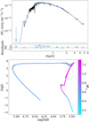 |
Fig. 1 Stellar characterisation for one of the targets in our sample. Upper panel: SED fit for S1429. Datapoints in blue are flux values from available broadband photometry with the error in the x-axis direction corresponding to the passband of the filter and the y-error corresponding to the 1σ uncertainties of the flux. The best-fitting Phoenix model is plotted in black. Purple diamonds represent the flux value of the synthetic photometry from the Phoenix model in each passband. The residuals normalised to the errors of the photometry are shown below. Lower panel: isochrone fit for S1429. |
3.2.2 Stars included in the original sample
We included 7 stars from the original 88 in our sample to be observed with HPF. All of them show either long-term trends or potential planetary signals in their RVs, which we were hoping to track with HPF; where this was successful, we were able to determine a minimum mass and period for the companion.
To observe the long-term trend, it was preferable to sacrifice precision in order to obtain relatively accurate calibrated RVs as the fitting of the offset with RVSearch is not very constrained when the observation window spans less than one period, especially for the relatively low number of observations we have for this work. We therefore derived our HPF RVs using the same Phoenix template from Sec. 2.1 and corrected them to the zero point of HARPS using the calculated offset. In the following periodogram analysis, all observations are treated as coming from the same instrument. Of the seven datasets, three do not show a significant peak in the periodogram from RVSearch. For S488, S1557, and YBP1137, the quality of the HPF spectra is not high enough, as the error on the RV points is as large as the amplitude of the trend we want to observe.
For the other four targets, RVSearch detects a significant periodicity in the data. However, all of the peaks in the periodograms are at periods larger than the observational baseline. This causes the MCMC to fail in returning a well-sampled posterior in three cases (S815, YBP778, and YBP1062), which results in unrealistic errors for the periods that are larger than the periods themselves. A similar behaviour was noted by Laliotis et al. (2023), where the treatment of signals with periods larger than the observational baseline proved problematic. While the periodogram can only fully resolve periods shorter than the observational baseline, the MCMC is not subject to this limitation and therefore fails to return a well-sampled posterior. Appendix shows the plotted RVs and periodograms including the data from Brucalassi et al. (2017) for the targets where no significant periodic signals are found.
For YBP2018, the MCMC did converge and produced a distinct solution, albeit with relatively large errors. Figure 2 summarises the results from RVSearch. In Brucalassi et al. (2017), YBP2018 was presented as a potential planet candidate with a peak-to-peak RV variation of 400 m s−1 and a tentative Keplerian solution with a period of ~2487 days. With our new data, we can rule out a planetary companion, as they show that the star has a much larger orbital period of 12574 ± 2400 days and an RV amplitude of 1947 ± 510 m s−1. As seen in panel e of Fig. 2, the significance of the RV signal strongly increases after the inclusion of our new data in the fit. Given the mass of 1.03 M⊙ for YBP2018, the companion has a minimum mass of 0.22 ± 0.06 M⊙.
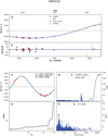 |
Fig. 2 RVSearch summary plot for YBP 2018. Panel a shows the RV time-series with the best-fit model with the residuals shown in panel b. Datapoints labelled HRS are from the old high-resolution spectrograph installed at the HET. All of the RV observations are corrected to the zero point of HARPS and are therefore treated as coming from one instrument. Panel c shows the phase-folded RV curve with the values derived from the MCMC. Panels d and f show the periodogram of the one- and two-planet models and panel e plots the significance of the RV signal as a function of the number of observations. |
3.2.3 Potential stellar companions for S995 and S2207
S995 and S2207 are the first two stars in this paper that were not in the original sample of Pasquini et al. (2012). We started observations for both stars in December 2019. After the first year of observations, a large trend in the RVs of both stars was identified that is indicative of a stellar companion. These stars were therefore only sparsely observed going forward as the focus was set on the other three stars as potential planet hosts in the sample. In total, we collected 11 spectra for S995 and 14 spectra for S2207 with HPF. Additionally, we have two SOPHIE and two HARPS observations for S995 as well as six HARPS-North, two SOPHIE, and four HARPS spectra for S2207.
We used the same approach as that employed in the previous section for the seven stars of the original sample to search for periodicity and fit the potential orbits. The HPF RVs for both stars were calculated with a PHOENIX template and corrected to the zero point of HARPS. The periodogram for S995 has the highest peak at 365 days, with similar peaks at integer fractions and multiples of the signal (~90 days, ~730 days). No peak exceeds the 0.1% false-positive threshold, and looking at the RV data, the potential orbit appears to be highly eccentric (see Fig. B.3). Additional data are needed to find the correct period and orbital configuration for this potential companion.
The orbital fitting was successful for S2207, revealing a stellar companion with a period of 1882 ± 24 days, an eccentricity of 0.5 ± 0.13, and an amplitude of 2847 ± 860 m s−1. Figure 3 shows the summary of the results for this star. Given the derived mass for S2207, the companion would have a minimum mass of 0.17 ± 0.05 M⊙ The large error on the mass of the companion is due to the incomplete sampling of the curve and can be improved with future observations.
3.2.4 Radial velocity analysis of S1083 and S1268
The two stars S1083 and S1268 showed no large RV variations or trends in their early RV data and were therefore selected as candidates to host an exoplanet and were observed more thoroughly. We collected 31 and 37 spectra for S1083 and S1268, respectively. Additionally, 4 HARPS-North, 2 SOPHIE, and 3 HARPS observations are available for S1083, and 4 HARPS-North, 2 SOPHIE, and 2 HARPS observations for S1268. The HARPS spectra for S1083 show some anomalies that suggest that something went wrong either in the observation or the reduction. Two of the HARPS spectra are shifted by 550 m s−1 against the third one; both of those observations also have unusually small error bars at 1 m s−1. We therefore chose to ignore the HARPS observations for S1083 in the analysis.
As explained in Sec. 2.1, we used a template created from all HPF observations for the calculation of the HPF RV values with SERVAL to achieve the highest possible precision. During the periodogram analysis with RVSearch, we treat each of the four datasets separately with individual offsets and jitter terms. The results of the periodogram analysis together with plots of the RVs are shown in Figs. 4 and 5. Neither star has a significant periodicity in its RV data. The rms of the RVs is 64 m s−1 for S1083 and 49 m s−1 for S1268.
To investigate the completeness of our observations, we used the injection-recovery test implemented in RVSearch. We injected 3000 synthetic planet signals drawn from a log-uniform period and M sin i distribution into our data and tested whether they are recovered by the planet search algorithm. We chose an upper bound of 50000 days for the period and a lower bound of 0.1 m s−1 for the RV amplitude of our synthetic planets. As shown in Fig. A.1, our data were barely sensitive to planets larger than Jupiter in very close orbits and the sensitivity dropped quickly with increasing period. We are therefore not able to draw definitive conclusions as to the presence of planetary companions around S1083 and S1268.
3.2.5 Potential planetary signal around S1429
S1429 is the most observed star in our sample. Our dataset includes 9 spectra from HARPS-North observed between January 22 and January 28, 2017, 2 spectra from SOPHIE observed on 19 and 27 January 2017, 4 datapoints from HARPS between 13 December 2020 and 8 January 2021 and lastly 37 HPF spectra taken between 11 December 2019 and 13 February 2022. We excluded one data point for each of the HARPS, HARPS-North, and HPF spectra, as these have a much lower S/N than the average for the respective dataset. The initial RVs showed no large variations indicative of stellar companions, which made S1429 one of the three main targets for a planetary companion. As with S1083 and S1268, we constructed a high-S/N template using all 36 HPF spectra and fit individual offsets and jitter terms for each instrument during the periodogram analysis.
The periodogram shows a clear peak exceeding the 0.1% FAP at 77 days (see Fig. 6). This peak is also the strongest periodic signal when the HPF data are analysed without the other datasets, although the FAP in this case is larger than 0.1%. When combining only the HPF and HARPS-N spectra, which are the two largest datasets for this object, the threshold of 0.1% FAP is already exceeded. As the iterative periodogram search did not return a second significant periodic signal, RVSearch fits a single-planet Keplerian model to the data and samples the posterior distribution with an MCMC. The resulting fit is shown in Fig. 6.
The fit gives a non-zero eccentricity of 0.23. However, it is also consistent with zero at the 1σ level. To investigate whether this eccentricity is significant or the product of a bias towards non-zero eccentricities in the fitting of Keplerian orbits, we reanalysed our RV data with the Python package Juliet (Espinoza et al. 2019). Juliet is built to compare models fit to photometric or RV data for exoplanet detection by sampling Bayesian posteriors and evidence using nested sampling algorithms. The Bayesian evidence (ln Z) can be used to compare different models, with a Δ ln Z > 2 being the threshold for a moderate preference and a Δ ln Z > 5 being the threshold for a strong preference of one model over the other (Trotta 2008). As it focuses on evidence calculations, one of the drawbacks of nested sampling is that the posterior distribution is a by-product and might not be explored as efficiently. To compensate for this, Higson et al. (2019) proposed a modification to the standard nested sampling algorithm where, instead of keeping the number of live points constant, they are dynamically changed to adjust the focus during the run. This dynamic nested sampling algorithm is implemented in Juliet through the Python code dynesty (Speagle 2020).
We performed two separate fits, one with eccentricity and argument of periastron ω fixed to 0 and 90°, respectively, and one where both parameters are varied freely over a range of uniform priors. We imposed a Gaussian prior on the relative offsets γ of the RVs between the datasets centred around the values derived from the RVSearch periodogram analysis with the variance taken as the standard deviation of the RVs for the respective spectrographs. We used uniform priors for the RV amplitude K, the period, and the time of superior conjunction Tc. The results of the two fits are shown in Table 3. The Bayesian evidence slightly favours the circular model with a Δ ln Z of 1.8; however, with such a small difference in evidence, the preference for the circular model is barely statistically significant. This is likely due to the incomplete sampling at the maximum of the phase-folded RV curve (see Fig. 7), which limits the precision with which we can determine the eccentricity. The resulting corner plots for the two fits are shown in Appendix C. For all parameters, the mean values are very close to the maximum of the distribution. However, the eccentricity could not be constrained as well as the other parameters and shows a slightly wider distribution.
4 Discussion
4.1 Validation of the S1429 signal
We examined several activity indicators in order to verify that the periodic signal in the RV of S1429 is caused by a planetary companion and is not due to the effects of stellar activity. For each one, we checked whether we can find a periodic variation exactly at the period found in the RV data or an integer alias of that period. The first two activity indicators that we used are the Ca II infrared triplet (IRT) and the differential line width (dLW). Both are computed from the HPF spectra with SERVAL. The Ca II IRT has been shown to be a good indicator for tracking magnetic activity on the stellar surface, which changes the depth of the line cores at a period corresponding to the rotational period of the star (Fuhrmeister et al. 2019). The differential line width is calculated by SERVAL as a proxy for the mean stellar line profile, where variations of the line widths and shapes can be caused either by processes intrinsic to the star (pulsation, magnetic activity) or systematic effects of the instrument (for an in-depth explanation see Zechmeister et al. 2018). In either case, a correlation of the dLW with the RV variations would point to a source that is not planetary in nature. To ensure that we treat all of our spectroscopic signals the same, we used RVSearch to compute periodograms with the same uninformed approach that was used for the RVs to find periodicities in the Ca II IRT and dLW data.
For some of our data, the signal in the third line in the Ca triplet was too low to fit the line. Therefore, only 19 of the 36 possible observations could be used for the periodogram. The results are shown in Fig. 8. Both activity indicators show no periodicity at the orbital period of our planet candidate or at any integer aliases. The first two Ca II triplet lines have their peaks at 20 days and 32 days, respectively, with the 20 day period being a 365 day alias of the 32 day period for the second Ca line. The third Ca II IRT line and the differential line width also have peaks at the 20 day period, but for both, those are slightly lower than their highest peaks at 7 and 4.6 days. However, none of the signals are strong enough to be statistically significant. This is somewhat expected, as stars in M 67 are shown to have low amounts of chromospheric activity due to the relatively old age of the open cluster (Pace & Pasquini 2004).
In addition to these two spectroscopic activity indices, we also examine the TESS light curve of S1429 to check for periodic variations in the brightness that could be caused by star spots rotating with the star. Light curves of S1429 were produced as TESS-SPOC High-Level Science Products (Caldwell et al. 2020) by the TESS Science Processing Operation Center pipeline (SPOC, Jenkins et al. 2016) from the ten-minute cadence full frame images. The SPOC light curves give two flux values, the simple aperture photometry (SAP) flux and the presearch data conditioning simple aperture photometry flux (PDCSAP; Smith et al. 2012; Stumpe et al. 2012, 2014), which corrects the SAP data for signals caused by instrumental effects. As the PDCSAP light curves are optimised to detect transit signals from exoplanets, it is possible that the applied corrections also remove longer periodic stellar trends and not only instrumental systematics (Mathys et al. 2024). In cases where the expected rotation period is larger than 20 days, it can be better to use the SAP light curves if the stellar signal is not masked by such uncertainties. However, upon inspection of the light curve, the SAP flux shows strong trends from instrumental systematic uncertainties, which makes the detection of potential stellar rotation signals difficult. We therefore decided to use the PDCSAP light curves for our periodogram analysis, which we downloaded with the Python package lightkurve (Lightkurve Collaboration 2018). We again use RVSearch to look for periodicities in the photometric data (see Fig. 8). The highest peak is at 5.3 days, but a lower peak around the 20 day signal is visible, which was seen for the spectroscopic activity indicators.
Additionally, we search the light curve for transit events. Given the derived period and T0 with their respective uncertainties, we expect the transit to occur at the beginning of the second half of Sector 45 between 2459 539.06 BJD and 2459 543.04 BJD. For the first 24 h of this window, there is a gap in the light curve, but no transits can be found in the rest. Given the properties of the S1429 system, this would indicate an orbital inclination of <88.5°.
The rotational velocity of S1429 in the literature is given as v sin i ~ 5 km s−1 (Jönsson et al. 2020). Assuming an inclination of ~90° combined with the derived stellar radius of 2.13 R⊙ would result in a rotational period of ~21 days. The 20 day signal is therefore a realistic candidate for the rotational period of the star, although it should be noted that while the uncertainty for ν sin i is not given by Jönsson et al. (2020), it is typically of the order of a couple of km s−1, and so we expect this estimated period to be of limited accuracy.
As all of our activity indicators do not overlap with the period derived from the RV analysis, we conclude that our signal is most likely caused by the presence of a planet hereinafter referred to as S1429 b.
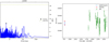 |
Fig. 4 Periodograms (left) and RV time-series (right) of S1083. The period value for the highest peak and the ΔBIC value for the 0.1% FAP are highlighted in black and yellow in the periodogram plot, respectively. |
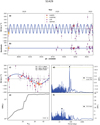 |
Fig. 6 Same as Fig. 2 but for S1429. For S1429, observations coming from the different instruments are fitted with separate offsets and jitter terms to take into account differences between the spectrographs. |
Summary of the Juliet fit to the RV data of S1429.
 |
Fig. 7 Phase-folded RV orbits for S1429 derived from the fit with Juliet. The left shows the orbit for a circular model, while on the right eccentricity is left to vary freely between 0 and 1. |
4.2 Planet properties in M 67
S1429 b is the sixth planet to be discovered in M 67, with the other five being presented in Brucalassi et al. (2017). Given the mass of the host star from Sec. 3.1, we calculate a minimum mass of 1.80 ± 0.2 MJ for S1429 b assuming a circular orbit. Using the orbital period and stellar properties, we derive a semimajor axis of 0.384 ± 0.004 au3 and an equilibrium temperature of 683 ± 9 K. With these properties, S1429 b falls into the class of warm-Jupiters (P ~ 10–200 days). Similarly to hot-Jupiters, these objects are thought to form at larger separations before migrating inwards, making them a secondary probe to test different migration theories. However, there are some key differences between the two populations, such as the prevalence of close-by and long-period companions or the distribution of eccentricities, which indicates that multiple different mechanisms are responsible for the variety of close-in giant planets (for a summary see e.g. Dawson & Johnson 2018). In total, we have now found three hot-Jupiters and three planets that belong to the warm/cold Jupiter class in M67.
The main advantage of studying planets inside star clusters is the homogeneity in chemical composition and age of the host stars, making it easier to discover the underlying reason for certain trends in the exoplanet population. Figure 9 shows the location of all the discovered M 67 planets in the mass–period distribution of known giant exoplanets (M sin i > 0.3 MJ) with host stars similar to the M 67 stars. For this plot, we downloaded data on all known exoplanets from the NASA Exoplanet Archive and filtered them according to the age (3.8–4.5 Gyr) and metallicity (−0.1–0.1) of M 67. A notable difference in planetary mass can be seen between the three hot-Jupiters and the three farther-out planets in M 67, with the planets at larger separations having a minimum mass that is between four and five times larger. The same trend is visible in the sample of planets around M 67-like stars, and even in the whole exoplanet population, where the short-period planets clump around lower mass values. Planets at longer periods, on the other hand, have a more homogenous mass distribution with a similar number of low- and high-mass planets.
This trend of an increase in planetary mass with larger orbital periods was reported in some of the early statistical works (Udry et al. 2003). However, recent studies using the California Legacy Survey (CLS) catalogue, which is based on a blind RV search of 719 FGKM stars spanning over three decades (Rosenthal et al. 2021), have suggested that both hot-Jupiters and farther-out giant planets follow a similar mass distribution, with the early differences in the distribution coming from observational biases whereby more massive planets at larger separations are more likely to be detected (Zink & Howard 2023).
We also find a correlation between the mass of the planet and the mass of its host star in M 67 (see Fig. 9), with more massive host stars hosting more massive planets. While a similar trend might be present for the M 67-like stars, in the full exoplanet population there seems to be no dependence of planetary mass on host-star mass. If this correlation were found to be real and not caused by a small or biased sample, this would suggest that it only holds true for a certain subset of stars; for example, solar metallicity stars with stars outside of this subset showing a different or no correlation between the masses.
However, as the detection of less massive planets gets more difficult for both larger separations and larger host-star masses, the lack of lower-mass giant planets at larger orbital periods and around more massive stars in our sample may stem from a detection bias. We use the same injection recovery tests presented in Sect. 3.2.4 to investigate the completeness of the datasets for the planet hosts in M 67. The completeness contour plots for each of the six planet hosts in M 67 are shown in Fig. A.1. The results of our injection recovery test show that the sensitivity of our datasets for planets with M sin i below one Jupiter mass drops rapidly for increasing periods and most smaller giants could not be recovered at periods larger than 10–20 days. This suggests that the larger masses we find for the farther-out planets could stem from a detection bias towards more massive planets. Similarly, the sensitivity of our RV data around the three more massive stars (S364, S978, and S1429) is significantly lower for less massive planets, especially in the cases of S364 and S1429 compared to the lower-mass stars. Therefore, the correlation between planetary and stellar mass is also expected given our data. Nevertheless, it is still noteworthy that all three hot-Jupiters in M 67 have minimum masses significantly below one Jupiter mass, as these types of planets are detectable in all our datasets.
One anomaly concerning the planets in M 67 is the rather large eccentricity for the three hot-Jupiters. Figure 9 shows the eccentricity distribution of giant planets (M sin i > 0.3 MJ) as a function of orbital period. While moderate eccentricities for the warm/cold Jupiters in M 67 are expected, as this population of exoplanets is known to have a broad eccentricity distribution (Dong et al. 2021), hot-Jupiters tend to favour circular orbits due to tidal circularisation effects caused by the proximity to the host star. Considering all exoplanets with periods between 1 and 10 days, the average eccentricity is ~0.07. This value does not change significantly when only considering the sample of ‘M 67-like’ stars. The three hot-Jupiters in M 67 all have larger-than-average eccentricities, with YBP1194 b (e = 0.31 ± 0.08) and YBP1514 b (e = 0.27 ± 0.09) having the most eccentric orbits out of the planets in the sample of M 67-like stars. However, looking at the eccentricities of close-in planets, the distribution appears to broaden with increasing period. Indeed, when we split the hot-Jupiter population into two period bins (1 < P < 5 and 5 < P < 10), the average eccentricity is considerably higher for the longer periods at 0.12 compared to 0.05. The distribution is also slightly broader with a higher standard deviation (0.15 vs. 0.10). Considering that both YBP1194 b and YBP1514 b have periods of longer than 5 days, the higher eccentricity values do not necessarily point towards a drastically different formation and evolution history of the M 67 giants compared to planets around field stars. Studies have shown that the majority of hot-Jupiters have a long-period giant companion (Knutson et al. 2014; Bryan et al. 2016; Zink & Howard 2023), which could disturb the orbit of the hot-Jupiter, especially at larger separations where the tidal forces from the star weaken. In the case of M 67, we do not detect any hint of long-term RV variation around the three hot-Jupiter hosts; although, as seen in Fig. A.1, the present data are only sensitive to planetary mass objects out to periods of ~2000–3000 days, and even then only for masses significantly above one Jupiter mass. As we cannot rule out the presence of outer perturbing giant planets, a dedicated follow-up campaign to search for outer companions could provide insights into whether the same migration mechanisms as in field stars are responsible for the shaping of hot-Jupiter systems in M 67 or if other dynamical interactions are at play in the dense cluster, such as stellar flybys (Malmberg et al. 2011; Shara et al. 2016; Wang et al. 2022).
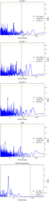 |
Fig. 8 Periodograms of the activity indicators derived from the HPF spectra and the photometric data from TESS. The first three plots show the periodicity in the signals of the calcium triplet lines. The fourth and fifth panels show the periodograms for the differential line width from SERVAL and the TESS photometry, respectively. The horizontal yellow line indicates the 0.1% FAP threshold and the vertical black line shows the location of the potential planet signal in the RVs of S1429. |
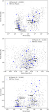 |
Fig. 9 Population of known giant exoplanets (M sin i > 0.3 MJ) with either a true mass or a M sin i measurement in planet mass–period (upper left) and planet mass–stellar mass (upper right) and eccentricity–period (lower panel) space using data from the NASA Exoplanet Archive. The full giant-planet population is shown in grey, while planets around stars with similar chemical composition and age as the stars in M 67 (−0.1 < Fe/H < 0.1 and 3.8 < age < 4.5) are shown in blue. The six planets discovered in M 67 are overplotted in black. |
4.3 Planet population at different evolutionary stages
The six planet hosts in M 67 are distributed over different evolutionary stages, with the three hot-Jupiters orbiting main sequence stars and the longer-period planets orbiting a turn-off point star and two red giants. The evolution of the host away from the main sequence and into a red giant is expected to significantly influence the surrounding planets and their orbits through tidal interaction, evaporation, or engulfment (see e.g. Villaver et al. 2014; Veras 2016). However, these interactions are still not well understood, particularly the point when the effects from stellar evolution start to become dominant and alter the planet population around them. We expect to learn a lot from studying planet hosts in different evolutionary states located in the same cluster, as not only can it be difficult to determine the exact point when a star evolves off the main sequence for field stars, but when studying the same cluster, we can also eliminate other factors such as system age and chemical composition, which can also affect the planet properties. For M 67, we find three short-period planets around main sequence stars but none around the more evolved stars. Unfortunately, our sample of planets in M 67 is far too small to come to any general conclusions as to the influence of stellar evolutionary state on planet properties.
To look for trends in the larger exoplanet population, we divided the list of planets from the previous section into three groups corresponding to host stars on the main sequence, stars that are in the process of evolving off the main sequence (sub-giants), and stars ascending the red-giant branch. We distinguish between the three evolutionary stages using the data-driven boundaries derived by Huber et al. (2016). Figure 10 shows the distribution of planet hosts into the three groups. We again focus on giant planets (M sin i > 0.3 MJ) and find a total of 971 planets around main sequence stars, 177 around subgiants, and 230 around giant stars with either a mass or M sin i measurement.
Looking at the distribution of exoplanets in mass–period space (Fig. 10), there appears to be no significant difference between the planet population around main sequence stars and that around subgiant stars. However, for the planets orbiting giant stars, there is a distinct lack of short-period planets. Additionally, except for one, all of the planets with periods of less than 10 days orbit giant stars at the beginning of the giant branch. In the plot, planets around these stars are marked with black edges around their markers. These results are consistent with recent occurrence rate analyses that find that the main sequence and subgiant occurrence rates are statistically indistinguishable and a paucity of short-period planets is only observed for stars that have significantly ascended the giant branch (Grunblatt et al. 2019; Temmink & Snellen 2023; Chontos et al. 2024).
This also seems to hold true for changes in the orbits of planets. As shown in Fig. 10, the orbital eccentricity follows a similar distribution for both main sequence and subgiant host stars with mean eccentricity and standard deviation values of 0.1 ± 0.16 for main sequence stars and 0.11 ± 0.17 for subgiants for planets with shorter periods (P < 100 days) and 0.34 ± 0.27 (subgiant hosts) and 0.30 ± 0.23 (main sequence hosts) for planets with periods of longer than 100 days. In the case of planet-hosting red giants, the mean eccentricities with their standard deviation are 0.12 ± 0.14 (P < 100 days) and 0.18 ± 0.17 (P > 100 days). While there is no significant difference for the close-in planets, at larger separations, circularisation effects of the orbits seem to be stronger for highly evolved stars, which is possibly due to stronger stellar tides.
These trends suggest that planets around main sequence and subgiant stars are very similar and are only affected significantly once the star has evolved further into the giant phase. However, as the exact evolutionary stage can be difficult to determine – especially for the subgiant phase –, a sample of well-characterised planet hosts across different stages of stellar evolution is needed in order to find the mechanisms that are responsible for shaping the different planet populations.
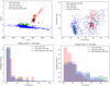 |
Fig. 10 Giant planet population around stars at different evolutionary stages. Upper left: host stars of giant exoplanets (M sin i > 0.3 MJ) with either a true mass or M sin i measurement divided into their evolutionary stage. Red points are giant stars, green points are subgiants, and blue points are main sequence stars. Red points with black edges are giant stars at the beginning of their ascension up the red giant branch (log g > 3.0). Upper right: population of giant exoplanets in mass–period space sorted by the evolutionary stage of their host star. Lower: Eccentricity distribution of planets with periods shorter than 100 days (left) and larger than 100 days (right) orbiting main sequence, subgiant, and giant stars. |
4.4 Hot-Jupiter occurrence in M 67
Lastly, we update the hot-Jupiter occurrence rate in M 67 using the method of Brucalassi et al. (2016) to include our five new targets. As discussed in the previous section, the planet populations around main sequence and turn-off or subgiant stars are very similar, which is why we consider both stellar types when calculating the hot-Jupiter occurrence rate. With no hot-Jupiters detected around the five new stars added to the sample, we derive an occurrence rate of ![Mathematical equation: $\[\4.2_{-2.3}^{+4.1}\]$](/articles/aa/full_html/2024/06/aa49233-24/aa49233-24-eq42.png) (compared to 4.5% before) and
(compared to 4.5% before) and ![Mathematical equation: $\[\5.4_{-3.0}^{+5.1}\]$](/articles/aa/full_html/2024/06/aa49233-24/aa49233-24-eq43.png) (compared to 5.6% before) when only considering single stars. These values are still higher than the 0.5–1% derived for field stars (Wright et al. 2012; Petigura et al. 2018; Zhou et al. 2019). We calculate both occurrence rates in order to be able to make comparisons with different survey strategies. Blind RV searches for planets often exclude binary star systems a priori, while transit surveys mostly do not make this kind of preselection. Because of this, occurrence rates from RV surveys have been higher than for transit surveys.
(compared to 5.6% before) when only considering single stars. These values are still higher than the 0.5–1% derived for field stars (Wright et al. 2012; Petigura et al. 2018; Zhou et al. 2019). We calculate both occurrence rates in order to be able to make comparisons with different survey strategies. Blind RV searches for planets often exclude binary star systems a priori, while transit surveys mostly do not make this kind of preselection. Because of this, occurrence rates from RV surveys have been higher than for transit surveys.
Given that M 67 was observed by TESS in sectors 34, 44, 45, and 46, it is possible to investigate whether the photometric data corroborate the higher hot-Jupiter occurrence rate of our RV survey.
We crosscheck a list of 1113 potential members of M 67 with the TESS input catalog and find that 320 have a light curve produced either by the SPOC (Jenkins et al. 2016) or the QLP (Huang et al. 2020) pipelines. Out of these 320 stars, none have a planet candidate in the TESS target-of-interest list. Assuming the occurrence rate of 4.2% for giant planets with periods of between 1 and 10 days derived from our RV survey and a transit probability of ![Mathematical equation: $\[\sim \frac{R_*}{a}\]$](/articles/aa/full_html/2024/06/aa49233-24/aa49233-24-eq44.png) , with R* being the stellar radius and a the semi-major axis, we would expect an average of ~1.2 transiting hot-Jupiters in the sample of 320 stars with TESS light curves. The calculation does not account for the ability to detect transit signals of hot-Jupiters in the given light curves, as a detailed completeness analysis for the 320 stars is beyond the scope of this work.
, with R* being the stellar radius and a the semi-major axis, we would expect an average of ~1.2 transiting hot-Jupiters in the sample of 320 stars with TESS light curves. The calculation does not account for the ability to detect transit signals of hot-Jupiters in the given light curves, as a detailed completeness analysis for the 320 stars is beyond the scope of this work.
Given that M 67 is a cluster, blending of neighbouring stars in the TESS apertures can complicate the detection of shallow transit signals, and so it might not be possible to recover planetary signals for all of the 320 stars, and the number of 1.2 expected transiting hot-Jupiters would be closer to an upper limit. However, there are techniques to reduce the blending in crowded fields, which could mitigate this issue (see Libralato et al. 2016; Nardiello et al. 2019). Therefore, the non-detection of hot-Jupiter signals in the TESS data of M 67 does not definitively disprove the higher occurrence rate derived during this survey.
5 Summary
We report spectroscopic data from an extension of the ‘Search for giant planets in M 67’ (Pasquini et al. 2012; Brucalassi et al. 2014, 2016, 2017) survey collected with the HPF spectrograph between 2019 and 2022. These data result in the detection of a new planet around the turn-off point star S1429. S1429 b is almost twice as massive as Jupiter at M sin i = 1.80 ± 0.2 MJ and has a period of ![Mathematical equation: $\[\77.48_{-0.19}^{+0.18}\]$](/articles/aa/full_html/2024/06/aa49233-24/aa49233-24-eq45.png) days assuming a circular orbit, but we cannot rule out a small eccentricity of the orbit. Given the derived properties, S1429 b belongs to the class of warm-Jupiters with an equilibrium temperature of 683 ± 9 K
days assuming a circular orbit, but we cannot rule out a small eccentricity of the orbit. Given the derived properties, S1429 b belongs to the class of warm-Jupiters with an equilibrium temperature of 683 ± 9 K
We also report two new candidates for binary star systems in S995 and S2207. For S2207, we find an orbital solution with a period of 1882 ± 24 days and a minimum mass of the companion of 0.17 ± 0.05 M⊙. Due to the incomplete sampling, we were not able to derive a definitive orbital solution for S995. Furthermore, the additional data confirm that a potential planetary signal in the RV of YBP2018 is caused by a stellar-mass companion with a minimum mass of 0.22 ± 0.06 M⊙.
M 67 remains an interesting target for studying exoplanets with a relatively homogeneous sample of host stars. In particular, the increased hot-Jupiter occurrence and the higher eccentricity distribution for the hot-Jupiters in M 67 warrant further investigation, either with detailed analysis of the available photometric data or additional RV observations.
Acknowledgements
We thank the anonymous referee for corrections and suggestions that helped us improve the presentation of the paper. L.T. acknowledges support from the Excellence Cluster ORIGINS funded by the Deutsche Forschungsgemeinschaft (DFG, German Research Foundation) under Germany’s Excellence Strategy – EXC 2094 – 390783311. R.P.S., L.P., A.B. thank ESO. R.P.S. thanks the Hobby Eberly Telescope (HET) project and CNRS for allocating the observations and the technical support. These results are based on observations obtained with the Habitable-zone Planet Finder Spectrograph on the HET. The HPF team acknowledges support from NSF grants AST-1006676, AST-1126413, AST-1310885, AST-1517592, AST-1310875, ATI 2009889, ATI-2009982, AST-2108512, and the NASA Astrobiology Institute (NNA09DA76A) in the pursuit of precision radial velocities in the NIR. The HPF team also acknowledges support from the Heising-Simons Foundation via grant 2017-0494. The Hobby-Eberly Telescope is a joint project of the University of Texas at Austin, the Pennsylvania State University, Ludwig-Maximilians-Universität München, and Georg-August Universität Gottingen. The HET is named in honor of its principal benefactors, William P. Hobby and Robert E. Eberly. The HET Collaboration acknowledges the support and resources from the Texas Advanced Computing Center. We thank the Resident Astronomers and Telescope Operators at the HET for the skillful execution of our observations with HPF. We would like to acknowledge that the HET is built on Indigenous land. Moreover, we would like to acknowledge and pay our respects to the Carrizo & Comecrudo, Coahuiltecan, Caddo, Tonkawa, Comanche, Lipan Apache, Alabama-Coushatta, Kickapoo, Tigua Pueblo, and all the American Indian and Indigenous Peoples and communities who have been or have become a part of these lands and territories in Texas, here on Turtle Island. AB thanks the GAPS-TNG community. HLR acknowledges the support of the DFG priority program SPP 1992 Exploring the Diversity of Extrasolar Planets (RE 1664/20-1). We acknowledge support from the Programme National de Physique Stellaire and the Programme National de Planétologie of the Institut National des Sciences de l’Univers – CNRS that allocated the observation time at the OHP 1.93 m telescope. J.R.M., B.L.C.M., and I.C.L. acknowledge partial financial support from the Brazilian funding agencies CNPq, Print/CAPES/UFRN, and CAPES (Finance Code 001). The HARPS data used in this work was collected via the programs 106.215E.002 and 106.215E.004. This research has made use of the NASA Exoplanet Archive, which is operated by the California Institute of Technology, under contract with the National Aeronautics and Space Administration under the Exoplanet Exploration Program. We acknowledge the use of public TESS data from pipelines at the TESS Science Office and at the TESS Science Processing Operations Center. Funding for the TESS mission is provided by NASA’s Science Mission Directorate. This research has made use of the Exoplanet Follow-up Observation Program website, which is operated by the California Institute of Technology, under contract with the National Aeronautics and Space Administration under the Exoplanet Exploration Program. Resources supporting this work were provided by the NASA High-End Computing (HEC) Program through the NASA Advanced Supercomputing (NAS) Division at Ames Research Center for the production of the SPOC data products. This paper includes data collected by the TESS mission that are publicly available from the Mikulski Archive for Space Telescopes (MAST).
Appendix A Injection recovery plots
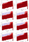 |
Fig. A.1 Injection recovery tests for S1083 and S1268 (top row) and all planet hosts in M 67 (other rows). The blue data points are injected signals that could be recovered by RVSearch, while the red data points were not recovered when injected into the RV data. The horizontal black dotted lines are at 1 Jupiter mass and at the brown dwarf limit (13 MJ). For detected planets, the location is indicated by the black cross. |
Appendix B Periodogram and RV plots
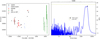 |
Fig. B.1 Results of the RV analysis for S488. Left: Time-series of the RVs for S488. All RV values are corrected to the zero point of HARPS as described in the paper. Right: Result of the periodogram analysis with RVSearch. |
Appendix C Juliet corner plots
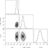 |
Fig. C.1 Corner plot of the Juliet fit with fixed eccentricity and argument of periastron. |
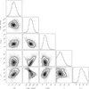 |
Fig. C.2 Corner plot of the Juliet fit where eccentricity and ω are allowed to vary freely. |
Appendix D Radial velocity tables
Radial velocities for S1429. All RVs are corrected to the zero point of HARPS using the offset derived with the Juliet fitting.
Radial velocities for S1083. All RVs are corrected to the zero point of HARPS using the offset derived from the periodogram analysis with RVSearch.
Radial velocities for S1268. All RVs are corrected to the zero point of HARPS using the offset derived from the periodogram analysis with RVSearch.
Radial velocities for YBP778. HPF RVs are corrected to the zero point of HARPS using the offset derived in Section 2.1.
Radial velocities for YBP1062. HPF RVs are corrected to the zero point of HARPS using the offset derived in Section 2.1.
Radial velocities for YBP1137. HPF RVs are corrected to the zero point of HARPS using the offset derived in Section 2.1.
Radial velocities for YBP2018. HPF RVs are corrected to the zero point of HARPS using the offset derived in Section 2.1.
Radial velocities for S488. HPF RVs are corrected to the zero point of HARPS using the offset derived in Section 2.1.
Radial velocities for S815. HPF RVs are corrected to the zero point of HARPS using the offset derived in Section 2.1.
Radial velocities for S995. HPF RVs are corrected to the zero point of HARPS using the offset derived in Section 2.1.
Radial velocities for S1557. HPF RVs are corrected to the zero point of HARPS using the offset derived in Section 2.1.
Radial velocities for S2207. HPF RVs are corrected to the zero point of HARPS using the offset derived in Section 2.1.
References
- Allard, F., Homeier, D., & Freytag, B. 2012, Philos. Trans. R. Soc. A, 370, 2765 [NASA ADS] [CrossRef] [Google Scholar]
- Anglada-Escudé, G., & Butler, R. P. 2012, ApJS, 200, 15 [Google Scholar]
- Barragán, O., Aigrain, S., Kubyshkina, D., et al. 2019, MNRAS, 490, 698 [Google Scholar]
- Bitsch, B., Trifonov, T., & Izidoro, A. 2020, A&A, 643, A66 [EDP Sciences] [Google Scholar]
- Borucki, W. J., Koch, D., Basri, G., et al. 2010, Science, 327, 977 [Google Scholar]
- Bouchy, F., Díaz, R. F., Hébrard, G., et al. 2013, A&A, 549, A49 [NASA ADS] [CrossRef] [EDP Sciences] [Google Scholar]
- Brucalassi, A., Pasquini, L., Saglia, R., et al. 2014, A&A, 561, L9 [NASA ADS] [CrossRef] [EDP Sciences] [Google Scholar]
- Brucalassi, A., Pasquini, L., Saglia, R., et al. 2016, A&A, 592, L1 [NASA ADS] [CrossRef] [EDP Sciences] [Google Scholar]
- Brucalassi, A., Koppenhoefer, J., Saglia, R., et al. 2017, A&A, 603, A85 [NASA ADS] [CrossRef] [EDP Sciences] [Google Scholar]
- Bryan, M. L., Knutson, H. A., Howard, A. W., et al. 2016, ApJ, 821, 89 [NASA ADS] [CrossRef] [Google Scholar]
- Caldwell, D. A., Tenenbaum, P., Twicken, J. D., et al. 2020, Res. Notes AAS, 4, 201 [NASA ADS] [CrossRef] [Google Scholar]
- Castelli, F., & Kurucz, R. L. 2003, IAU Symp., 210, A20 [Google Scholar]
- Choi, J., Dotter, A., Conroy, C., et al. 2016, ApJ, 823, 102 [Google Scholar]
- Chontos, A., Huber, D., Grunblatt, S. K., et al. 2024, arXiv e-prints [arXiv:2402.07893] [Google Scholar]
- Currie, T. 2009, ApJ, 694, L171 [Google Scholar]
- David, T. J., Hillenbrand, L. A., Petigura, E. A., et al. 2016, Nature, 534, 658 [CrossRef] [Google Scholar]
- David, T. J., Cody, A. M., Hedges, C. L., et al. 2019a, ApJ, 158, 79 [CrossRef] [Google Scholar]
- David, T. J., Petigura, E. A., Luger, R., et al. 2019b, ApJ, 885, L12 [Google Scholar]
- Dawson, R. I., & Johnson, J. A. 2018, ARA&A 56, 175 [Google Scholar]
- De Silva, G., Freeman, K., Asplund, M., et al. 2007, AJ, 133, 1161 [NASA ADS] [CrossRef] [Google Scholar]
- Dong, J., Huang, C. X., Zhou, G., et al. 2021, ApJ, 920, L16 [NASA ADS] [CrossRef] [Google Scholar]
- Dotter, A. 2016, ApJS, 222, 8 [Google Scholar]
- Espinoza, N., Kossakowski, D., & Brahm, R. 2019, MNRAS, 490, 2262 [Google Scholar]
- Fischer, D. A., & Valenti, J. 2005, ApJ, 622, 1102 [NASA ADS] [CrossRef] [Google Scholar]
- Foreman-Mackey, D., Hogg, D. W., Lang, D., & Goodman, J. 2013, PASP, 125, 306 [Google Scholar]
- Fortney, J. J., Dawson, R. I., & Komacek, T. D. 2021, J. Geophys. Res. Planets, 126, e2020JE006629 [CrossRef] [Google Scholar]
- Fuhrmeister, B., Czesla, S., Schmitt, J. H., et al. 2019, A&A, 623, A24 [NASA ADS] [CrossRef] [EDP Sciences] [Google Scholar]
- Fulton, B. J., Petigura, E. A., Blunt, S., & Sinukoff, E. 2018, PASP, 130, 044504 [Google Scholar]
- Ghezzi, L., Montet, B. T., & Johnson, J. A. 2018, ApJ, 860, 109 [Google Scholar]
- Goldreich, P., & Tremaine, S. 1980, ApJ, 241, 425 [Google Scholar]
- Gonzalez, G. 1997, MNRAS, 285, 403 [Google Scholar]
- Grunblatt, S. K., Huber, D., Gaidos, E., et al. 2019, AJ, 158, 227 [Google Scholar]
- Hamers, A. S., & Tremaine, S. 2017, AJ, 154, 272 [NASA ADS] [CrossRef] [Google Scholar]
- Higson, E., Handley, W., Hobson, M., & Lasenby, A. 2019, Stat. Comput., 29, 891 [Google Scholar]
- Hill, G. J., Lee, H., MacQueen, P. J., et al. 2021, AJ, 162, 298 [NASA ADS] [CrossRef] [Google Scholar]
- Horne, K. 1986, PASP, 98, 609 [Google Scholar]
- Howell, S. B., Sobeck, C., Haas, M., et al. 2014, PASP, 126, 398 [Google Scholar]
- Huang, C. X., Vanderburg, A., Pál, A., et al. 2020, Res. Notes AAS, 4, 204 [NASA ADS] [CrossRef] [Google Scholar]
- Huber, D., Bryson, S. T., Haas, M. R., et al. 2016, ApJS, 224, 2 [Google Scholar]
- Husser, T.-O., Wende-von Berg, S., Dreizler, S., et al. 2013, A&A, 553, A6 [NASA ADS] [CrossRef] [EDP Sciences] [Google Scholar]
- Ida, S., & Lin, D. 2008, ApJ, 673, 487 [NASA ADS] [CrossRef] [Google Scholar]
- Jenkins, J. M., Twicken, J. D., McCauliff, S., et al. 2016, SPIE, 9913, 1232 [Google Scholar]
- Jenkins, J. S., Jones, H., Tuomi, M., et al. 2017, MNRAS, 466, 443 [CrossRef] [Google Scholar]
- Johnson, J. A., Aller, K. M., Howard, A. W., & Crepp, J. R. 2010, PASP, 122, 905 [Google Scholar]
- Jönsson, H., Holtzman, J. A., Prieto, C. A., et al. 2020, AJ, 160, 120 [CrossRef] [Google Scholar]
- Kanodia, S., & Wright, J. 2018, Res. Notes AAS, 2, 4 [NASA ADS] [CrossRef] [Google Scholar]
- Kennedy, G. M., & Kenyon, S. J. 2009, ApJ, 695, 1210 [NASA ADS] [CrossRef] [Google Scholar]
- Knutson, H. A., Fulton, B. J., Montet, B. T., et al. 2014, ApJ, 785, 126 [NASA ADS] [CrossRef] [Google Scholar]
- Kurucz, R. 1993, ATLAS9 Stellar Atmosphere Programs and 2 km s−1 grid. Kurucz CD-ROM No. 13 (Cambridge: Cambridge University Press), 13 [Google Scholar]
- Laliotis, K., Burt, J. A., Mamajek, E. E., et al. 2023, AJ, 165, 176 [NASA ADS] [CrossRef] [Google Scholar]
- Li, D., Mustill, A. J., Davies, M. B., & Gong, Y.-X. 2023a, MNRAS, 527, 386 [CrossRef] [Google Scholar]
- Li, D., Mustill, A. J., Davies, M. B., & Gong, Y.-X. 2023b, MNRAS, 518, 4265 [Google Scholar]
- Libralato, M., Bedin, L. R., Nardiello, D., & Piotto, G. 2016, MNRAS, 456, 1137 [NASA ADS] [CrossRef] [Google Scholar]
- Lightkurve Collaboration (Cardoso, J. V. d. M., et al.) 2018, Astrophysics Source Code Library [record ascl:1812.013] [Google Scholar]
- Lin, D. N., & Papaloizou, J. 1986, ApJ, 309, 846 [NASA ADS] [CrossRef] [Google Scholar]
- Livingston, J. H., Dai, F., Hirano, T., et al. 2018, AJ, 155, 115 [NASA ADS] [CrossRef] [Google Scholar]
- Livingston, J. H., Dai, F., Hirano, T., et al. 2019, MNRAS, 484, 8 [NASA ADS] [CrossRef] [Google Scholar]
- Lovis, C., & Mayor, M. 2007, A&A, 472, 657 [NASA ADS] [CrossRef] [EDP Sciences] [Google Scholar]
- Mahadevan, S., Ramsey, L., Bender, C., et al. 2012, SPIE, 8446, 624 [Google Scholar]
- Mahadevan, S., Ramsey, L. W., Terrien, R., et al. 2014, SPIE, 9147, 543 [Google Scholar]
- Mahadevan, S., Anderson, T., Balderrama, E., et al. 2018, SPIE, 10702, 1070214 [Google Scholar]
- Malavolta, L., Nascimbeni, V., Piotto, G., et al. 2016, A&A, 588, A118 [NASA ADS] [CrossRef] [EDP Sciences] [Google Scholar]
- Malmberg, D., Davies, M. B., & Heggie, D. C. 2011, MNRAS, 411, 859 [Google Scholar]
- Mann, A. W., Gaidos, E., Mace, G. N., et al. 2016a, ApJ, 818, 46 [NASA ADS] [CrossRef] [Google Scholar]
- Mann, A. W., Newton, E. R., Rizzuto, A. C., et al. 2016b, AJ, 152, 61 [Google Scholar]
- Mann, A. W., Gaidos, E., Vanderburg, A., et al. 2017, AJ, 153, 64 [Google Scholar]
- Mathys, G., Holdsworth, D. L., & Kurtz, D. W., 2024, A&A, 683, A227 [NASA ADS] [CrossRef] [EDP Sciences] [Google Scholar]
- Mayor, M., & Queloz, D. 1995, Nature, 378, 355 [Google Scholar]
- Mayor, M., Pepe, F., Queloz, D., et al. 2003, The Messenger, 114, 20 [NASA ADS] [Google Scholar]
- Meibom, S., Torres, G., Fressin, F., et al. 2013, Nature, 499, 55 [NASA ADS] [CrossRef] [Google Scholar]
- Metcalf, A. J., Anderson, T., Bender, C. F., et al. 2019, Optica, 6, 233 [NASA ADS] [CrossRef] [Google Scholar]
- Morton, T. D. 2015, Astrophysics Source Code Library [record ascl:1503.010] [Google Scholar]
- Nardiello, D., Borsato, L., Piotto, G., et al. 2019, MNRAS, 490, 3806 [NASA ADS] [CrossRef] [Google Scholar]
- Ninan, J., Bender, C. F., Mahadevan, S., et al. 2018, SPIE, 10709, 694 [Google Scholar]
- Obermeier, C., Henning, T., Schlieder, J. E., et al. 2016, AJ, 152, 223 [NASA ADS] [CrossRef] [Google Scholar]
- Önehag, A., Korn, A., Gustafsson, B., Stempels, E., & VandenBerg, D. A. 2011, A&A, 528, A85 [NASA ADS] [CrossRef] [EDP Sciences] [Google Scholar]
- Önehag, A., Gustafsson, B., & Korn, A. 2014, A&A, 562, A102 [NASA ADS] [CrossRef] [EDP Sciences] [Google Scholar]
- Pace, G., & Pasquini, L. 2004, A&A, 426, 1021 [NASA ADS] [CrossRef] [EDP Sciences] [Google Scholar]
- Pasquini, L., Randich, S., Zoccali, M., et al. 2004, A&A, 424, 951 [NASA ADS] [CrossRef] [EDP Sciences] [Google Scholar]
- Pasquini, L., Brucalassi, A., Ruiz, M., et al. 2012, A&A, 545, A139 [NASA ADS] [CrossRef] [EDP Sciences] [Google Scholar]
- Paulson, D. B., Cochran, W. D., & Hatzes, A. P. 2004, AJ, 127, 3579 [Google Scholar]
- Pepe, F., Mayor, M., Galland, F., et al. 2002, A&A, 388, 632 [NASA ADS] [CrossRef] [EDP Sciences] [Google Scholar]
- Perruchot, S., Kohler, D., Bouchy, F., et al. 2008, SPIE, 7014, 235 [Google Scholar]
- Petigura, E. A., Marcy, G. W., Winn, J. N., et al. 2018, AJ, 155, 89 [Google Scholar]
- Petrovich, C. 2015, ApJ, 805, 75 [NASA ADS] [CrossRef] [Google Scholar]
- Quinn, S. N., White, R. J., Latham, D. W., et al. 2012, ApJ, 756, L33 [NASA ADS] [CrossRef] [Google Scholar]
- Quinn, S. N., White, R. J., Latham, D. W., et al. 2014, ApJ, 787, 27 [NASA ADS] [CrossRef] [Google Scholar]
- Ramsey, L. W., Adams, M. T., Barnes, T. G., et al. 1998, SPIE Conf. Ser., 3352, 34 [Google Scholar]
- Randich, S., Bragaglia, A., Pastori, L., et al. 2005, The Messenger, 121, 18 [NASA ADS] [Google Scholar]
- Randich, S., Sestito, P., Primas, F., Pallavicini, R., & Pasquini, L. 2006, A&A, 450, 557 [NASA ADS] [CrossRef] [EDP Sciences] [Google Scholar]
- Rasio, F. A., & Ford, E. B. 1996, Science, 274, 954 [Google Scholar]
- Reffert, S., Bergmann, C., Quirrenbach, A., Trifonov, T., & Künstler, A. 2015, A&A, 574, A116 [NASA ADS] [CrossRef] [EDP Sciences] [Google Scholar]
- Rizzuto, A. C., Vanderburg, A., Mann, A. W., et al. 2018, AJ, 156, 195 [NASA ADS] [CrossRef] [Google Scholar]
- Rosenthal, L. J., Fulton, B. J., Hirsch, L. A., et al. 2021, ApJS, 255, 8 [NASA ADS] [CrossRef] [Google Scholar]
- Santos, N. C., Israelian, G., & Mayor, M. 2004, A&A, 415, 1153 [NASA ADS] [CrossRef] [EDP Sciences] [Google Scholar]
- Sato, B., Kambe, E., Takeda, Y., et al. 2005, PASJ, 57, 97 [Google Scholar]
- Sato, B., Izumiura, H., Toyota, E., et al. 2007, ApJ, 661, 527 [NASA ADS] [CrossRef] [Google Scholar]
- Sato, B., Izumiura, H., Toyota, E., et al. 2008, PASJ, 60, 539 [NASA ADS] [Google Scholar]
- Schlegel, D. J., Finkbeiner, D. P., & Davis, M. 1998, ApJ, 500, 525 [Google Scholar]
- Shara, M. M., Hurley, J. R., & Mardling, R. A. 2016, ApJ, 816, 59 [NASA ADS] [CrossRef] [Google Scholar]
- Smith, J. C., Stumpe, M. C., Van Cleve, J. E., et al. 2012, PASP, 124, 1000 [Google Scholar]
- Speagle, J. S. 2020, MNRAS, 493, 3132 [Google Scholar]
- Stumpe, M. C., Smith, J. C., Van Cleve, J. E., et al. 2012, PASP, 124, 985 [Google Scholar]
- Stumpe, M. C., Smith, J. C., Catanzarite, J. H., et al. 2014, PASP, 126, 100 [Google Scholar]
- Takarada, T., Sato, B., Omiya, M., Hori, Y., & Fujii, M. S. 2020, PASJ, 72, 104 [NASA ADS] [CrossRef] [Google Scholar]
- Temmink, M., & Snellen, I. A. 2023, A&A, 670, A26 [NASA ADS] [CrossRef] [EDP Sciences] [Google Scholar]
- Trotta, R. 2008, Contemp. Phys., 49, 71 [Google Scholar]
- Udry, S., Mayor, M., & Santos, N. 2003, A&A, 407, 369 [NASA ADS] [CrossRef] [EDP Sciences] [Google Scholar]
- Vanderburg, A., Mann, A. W., Rizzuto, A., et al. 2018, AJ, 156, 46 [NASA ADS] [CrossRef] [Google Scholar]
- Veras, D. 2016, R. Soc. Open Sci., 3, 150571 [Google Scholar]
- Villaver, E., & Livio, M. 2009, ApJ, 705, L81 [Google Scholar]
- Villaver, E., Livio, M., Mustill, A. J., & Siess, L. 2014, ApJ, 794, 3 [NASA ADS] [CrossRef] [Google Scholar]
- Vines, J. I., & Jenkins, J. S. 2022, MNRAS, 513, 2719 [NASA ADS] [CrossRef] [Google Scholar]
- Wang, Y.-H., Leigh, N. W., Perna, R., & Shara, M. M. 2020, ApJ, 905, 136 [NASA ADS] [CrossRef] [Google Scholar]
- Wang, Y.-H., Perna, R., Leigh, N. W., & Shara, M. M. 2022, MNRAS, 509, 5253 [Google Scholar]
- Wolthoff, V., Reffert, S., Quirrenbach, A., et al. 2022, A&A, 661, A63 [NASA ADS] [CrossRef] [EDP Sciences] [Google Scholar]
- Wright, J., Marcy, G., Howard, A., et al. 2012, ApJ, 753, 160 [NASA ADS] [CrossRef] [Google Scholar]
- Wu, Y., & Lithwick, Y. 2011, ApJ, 735, 109 [Google Scholar]
- Yadav, R., Bedin, L., Piotto, G., et al. 2008, A&A, 484, 609 [NASA ADS] [CrossRef] [EDP Sciences] [Google Scholar]
- Zechmeister, M., Reiners, A., Amado, P. J., et al. 2018, A&A, 609, A12 [NASA ADS] [CrossRef] [EDP Sciences] [Google Scholar]
- Zhou, G., Huang, C., Bakos, G., et al. 2019, AJ, 158, 141 [NASA ADS] [CrossRef] [Google Scholar]
- Zink, J. K., & Howard, A. W. 2023, ApJ, 956, L29 [Google Scholar]
Given the distance of ~1 kpc, this makes the reflex astrometric wobbling of the parent star undetectable even with the fifth Gaia Data Release.
All Tables
Number of observations of each star in our sample with the different spectrographs (the HPF spectrograph, H: HARPS, S: SOPHIE, HN: HARPS-North).
Stellar parameters derived from the SED analysis and MIST isochrones fit for the 11 stars in our sample.
Radial velocities for S1429. All RVs are corrected to the zero point of HARPS using the offset derived with the Juliet fitting.
Radial velocities for S1083. All RVs are corrected to the zero point of HARPS using the offset derived from the periodogram analysis with RVSearch.
Radial velocities for S1268. All RVs are corrected to the zero point of HARPS using the offset derived from the periodogram analysis with RVSearch.
Radial velocities for YBP778. HPF RVs are corrected to the zero point of HARPS using the offset derived in Section 2.1.
Radial velocities for YBP1062. HPF RVs are corrected to the zero point of HARPS using the offset derived in Section 2.1.
Radial velocities for YBP1137. HPF RVs are corrected to the zero point of HARPS using the offset derived in Section 2.1.
Radial velocities for YBP2018. HPF RVs are corrected to the zero point of HARPS using the offset derived in Section 2.1.
Radial velocities for S488. HPF RVs are corrected to the zero point of HARPS using the offset derived in Section 2.1.
Radial velocities for S815. HPF RVs are corrected to the zero point of HARPS using the offset derived in Section 2.1.
Radial velocities for S995. HPF RVs are corrected to the zero point of HARPS using the offset derived in Section 2.1.
Radial velocities for S1557. HPF RVs are corrected to the zero point of HARPS using the offset derived in Section 2.1.
Radial velocities for S2207. HPF RVs are corrected to the zero point of HARPS using the offset derived in Section 2.1.
All Figures
|
Fig. 1 Stellar characterisation for one of the targets in our sample. Upper panel: SED fit for S1429. Datapoints in blue are flux values from available broadband photometry with the error in the x-axis direction corresponding to the passband of the filter and the y-error corresponding to the 1σ uncertainties of the flux. The best-fitting Phoenix model is plotted in black. Purple diamonds represent the flux value of the synthetic photometry from the Phoenix model in each passband. The residuals normalised to the errors of the photometry are shown below. Lower panel: isochrone fit for S1429. |
| In the text | |
|
Fig. 2 RVSearch summary plot for YBP 2018. Panel a shows the RV time-series with the best-fit model with the residuals shown in panel b. Datapoints labelled HRS are from the old high-resolution spectrograph installed at the HET. All of the RV observations are corrected to the zero point of HARPS and are therefore treated as coming from one instrument. Panel c shows the phase-folded RV curve with the values derived from the MCMC. Panels d and f show the periodogram of the one- and two-planet models and panel e plots the significance of the RV signal as a function of the number of observations. |
| In the text | |
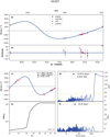 |
Fig. 3 Same as Fig. 2 but for S2207. |
| In the text | |
|
Fig. 4 Periodograms (left) and RV time-series (right) of S1083. The period value for the highest peak and the ΔBIC value for the 0.1% FAP are highlighted in black and yellow in the periodogram plot, respectively. |
| In the text | |
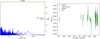 |
Fig. 5 Same as Fig. 4 but for S1268. |
| In the text | |
|
Fig. 6 Same as Fig. 2 but for S1429. For S1429, observations coming from the different instruments are fitted with separate offsets and jitter terms to take into account differences between the spectrographs. |
| In the text | |
|
Fig. 7 Phase-folded RV orbits for S1429 derived from the fit with Juliet. The left shows the orbit for a circular model, while on the right eccentricity is left to vary freely between 0 and 1. |
| In the text | |
|
Fig. 8 Periodograms of the activity indicators derived from the HPF spectra and the photometric data from TESS. The first three plots show the periodicity in the signals of the calcium triplet lines. The fourth and fifth panels show the periodograms for the differential line width from SERVAL and the TESS photometry, respectively. The horizontal yellow line indicates the 0.1% FAP threshold and the vertical black line shows the location of the potential planet signal in the RVs of S1429. |
| In the text | |
|
Fig. 9 Population of known giant exoplanets (M sin i > 0.3 MJ) with either a true mass or a M sin i measurement in planet mass–period (upper left) and planet mass–stellar mass (upper right) and eccentricity–period (lower panel) space using data from the NASA Exoplanet Archive. The full giant-planet population is shown in grey, while planets around stars with similar chemical composition and age as the stars in M 67 (−0.1 < Fe/H < 0.1 and 3.8 < age < 4.5) are shown in blue. The six planets discovered in M 67 are overplotted in black. |
| In the text | |
|
Fig. 10 Giant planet population around stars at different evolutionary stages. Upper left: host stars of giant exoplanets (M sin i > 0.3 MJ) with either a true mass or M sin i measurement divided into their evolutionary stage. Red points are giant stars, green points are subgiants, and blue points are main sequence stars. Red points with black edges are giant stars at the beginning of their ascension up the red giant branch (log g > 3.0). Upper right: population of giant exoplanets in mass–period space sorted by the evolutionary stage of their host star. Lower: Eccentricity distribution of planets with periods shorter than 100 days (left) and larger than 100 days (right) orbiting main sequence, subgiant, and giant stars. |
| In the text | |
|
Fig. A.1 Injection recovery tests for S1083 and S1268 (top row) and all planet hosts in M 67 (other rows). The blue data points are injected signals that could be recovered by RVSearch, while the red data points were not recovered when injected into the RV data. The horizontal black dotted lines are at 1 Jupiter mass and at the brown dwarf limit (13 MJ). For detected planets, the location is indicated by the black cross. |
| In the text | |
|
Fig. B.1 Results of the RV analysis for S488. Left: Time-series of the RVs for S488. All RV values are corrected to the zero point of HARPS as described in the paper. Right: Result of the periodogram analysis with RVSearch. |
| In the text | |
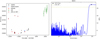 |
Fig. B.2 Same as Fig. B.1 but for S815. |
| In the text | |
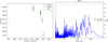 |
Fig. B.3 Same as Fig. B.1 but for S995. |
| In the text | |
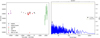 |
Fig. B.4 Same as Fig. B.1 but for S1557. |
| In the text | |
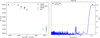 |
Fig. B.5 Same as Fig. B.1 but for YBP778. |
| In the text | |
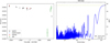 |
Fig. B.6 Same as Fig. B.1 but for YBP1062. |
| In the text | |
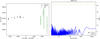 |
Fig. B.7 Same as Fig. B.1 but for YBP1137. |
| In the text | |
|
Fig. C.1 Corner plot of the Juliet fit with fixed eccentricity and argument of periastron. |
| In the text | |
|
Fig. C.2 Corner plot of the Juliet fit where eccentricity and ω are allowed to vary freely. |
| In the text | |
Current usage metrics show cumulative count of Article Views (full-text article views including HTML views, PDF and ePub downloads, according to the available data) and Abstracts Views on Vision4Press platform.
Data correspond to usage on the plateform after 2015. The current usage metrics is available 48-96 hours after online publication and is updated daily on week days.
Initial download of the metrics may take a while.