| Issue |
A&A
Volume 686, June 2024
|
|
|---|---|---|
| Article Number | A195 | |
| Number of page(s) | 14 | |
| Section | The Sun and the Heliosphere | |
| DOI | https://doi.org/10.1051/0004-6361/202349130 | |
| Published online | 12 June 2024 | |
Coupling between magnetic reconnection, energy release, and particle acceleration in the X17.2 2003 October 28 solar flare
1
Skobeltsyn Institute of Nuclear Physics, Lomonosov Moscow State University, Moscow 119991, Russia
2
Institute of Physics, University of Graz, Universitätsplatz 5, 8010 Graz, Austria
3
Kanzelhöhe Observatory for Solar and Environmental Research, University of Graz, Kanzelhöhe 19, 9521 Kanzelhöhe, Austria
4
Institute for Solar Physics-KIS, 79104 Freiburg, Germany
e-mail: This email address is being protected from spambots. You need JavaScript enabled to view it.
5
Center for Solar-Terrestrial research, Physics Dept., New Jersey Institute of Technology, Newark, NJ 07102, USA
6
Institute of Space Research, Austrian Academy of Sciences, Schmiedlstraße 6, 8042 Graz, Austria
7
Ioffe Institute, St. Petersburg 194021, Russia
Received:
29
December
2023
Accepted:
11
March
2024
Abstract
Context. The 2003 October 28 (X17.2) eruptive flare was a unique event. The coronal electric field and the π-decay γ-ray emission flux displayed the highest values ever inferred for solar flares.
Aims. Our aim is to reveal physical links between the magnetic reconnection process, energy release, and acceleration of electrons and ions to high energies in the chain of the magnetic energy transformations in the impulsive phase of the solar flare.
Methods. The global reconnection rate, φ̇(t), and the local reconnection rate (coronal electric field strength), Ec(r, t), were calculated from flare ribbon separation in Hα filtergrams and photospheric magnetic field maps. Then, HXRs measured by CORONAS-F/SPR-N and the derivative of the GOES SXR flux, İSXR(t) were used as proxies of the flare energy release evolution. The flare early rise phase, main raise phase, and main energy release phase were defined based on temporal profiles of the above proxies. The available results of INTEGRAL and CORONAS-F/SONG observations were combined with Konus-Wind data to quantify the time behavior of electron and proton acceleration. Prompt γ-ray lines and delayed 2.2 MeV line temporal profiles observed with Konus-Wind and INTEGRAL/SPI were used to detect and quantify the nuclei with energies of 10−70 MeV.
Results. The magnetic-reconnection rates, φ̇(t) and Ec(r, t), follow a common evolutionary pattern with the proxies of the flare energy released into high-energy electrons. The global and local reconnection rates reach their peaks at the end of the main rise phase of the flare. The spectral analysis of the high-energy γ-ray emission revealed a close association between the acceleration process efficiency and the reconnection rates. High-energy bremsstrahlung continuum and narrow γ-ray lines were observed in the main rise phase when Ec(r, t) of the positive (negative) polarity reached values of ∼120 V cm−1 (∼80 V cm−1). In the main energy release phase, the upper energy of the bremsstrahlung spectrum was significantly reduced and the pion-decay γ-ray emission appeared abruptly. We discuss the reasons why the change of the acceleration regime occurred along with the large-scale magnetic field restructuration of this flare.
Conclusions. The similarities between the proxies of the flare energy release with φ̇(t) and Ec(r, t) in the flare’s main rise phase are in accordance with the reconnection models. We argue that the main energy release and proton acceleration up to subrelativistic energies began just when the reconnection rate was going through the maximum, that is, following a major change of the flare topology.
Key words: Sun: activity / Sun: flares / Sun: magnetic fields / Sun: X-rays / gamma rays
© The Authors 2024
 Open Access article, published by EDP Sciences, under the terms of the Creative Commons Attribution License (https://creativecommons.org/licenses/by/4.0), which permits unrestricted use, distribution, and reproduction in any medium, provided the original work is properly cited.
This article is published in open access under the Subscribe to Open model. This email address is being protected from spambots. You need JavaScript enabled to view it. to support open access publication.
1. Introduction
Solar flares are energetic transient phenomena that involve several phases of energy transformation. After a complex preflare build up of the free magnetic energy in the solar corona, an instability leads to a sudden release of the free energy during a flare by magnetic reconnection driven by strong (likely turbulent) plasma flows (e.g., Chen et al. 2020) and accompanied by a strong dynamic electric field (Fleishman et al. 2020). The tracers of this released energy are the emission observed from radio to gamma-rays, solar energetic particles (SEPs), and coronal mass ejections (CMEs). A significant portion of the energy is spent on the acceleration of charged particles and plasma heating, which includes heating due to the collisional energy loss of the flare-accelerated particles (see, e.g., Martens & Young 1990; Litvinenko & Somov 1995; Veronig et al. 2005; Holman 2016; Fleishman et al. 2020, 2022) and direct heating (Gary & Hurford 1989; Caspi & Lin 2010; Caspi et al. 2014; Fleishman et al. 2015); see also the reviews by Fletcher et al. (2011), Vilmer et al. (2011), Holman et al. (2011), Somov (2013). However, it is not yet clear how exactly the magnetic energy release leads to the efficient acceleration of high-energy particles. The fundamental force capable of accelerating a charged particle is due to an electric field (see Jokipii 1979). This electric field in flares can be created by a variety of processes, such as a voltage drop at the reconnection site, MHD turbulence, or different kinds of MHD shock waves that are produced during flares (e.g., review by Miller et al. 1997). These accelerated high-energy electrons and protons produce various components of the nonthermal microwave, X-ray, and γ-ray spectrum (Bastian et al. 1998; Dermer & Ramaty 1986; Ramaty & Murphy 1987; Murphy et al. 1987), while the thermal plasma heated during the flare produces enhanced emission in the extreme ultra-violet (EUV) and soft X-ray (SXR) wavelength ranges.
Magnetic reconnection is an intrinsically three-dimensional (3D) process, and so, for the last twenty years, one of the main foci of researchers has been on the structure and dynamics of 3D reconnection (e.g., Li et al. 2021). Nevertheless, the quasi-2D, so called “standard flare model” (CSHKP, Carmichael 1964; Sturrock 1966; Hirayama 1974; Kopp & Pneuman 1976), which is a 2.5D configuration with translation symmetry, successfully explains the morphology of some eruptive flares, as well as quasi-parallel chromospheric ribbons and their divergent motion in the course of a flare. Within the CSHKP framework, a magnetic flux system can become unstable and at some point rise to higher coronal altitudes. Below it, a current sheet develops, towards which the ambient antiparallel magnetic field is brought in close contact and forced to reconnect (Priest & Forbes 2000; Forbes & Lin 2000; Vršnak 2016). Ribbons can be regarded as tracers of the low-atmosphere footpoints (FPs) of newly reconnected coronal magnetic field, since they are magnetically connected to the instantaneous coronal reconnection site. This permits the accelerated particles to precipitate to the chromosphere. As the reconnection region moves upwards, field lines anchored at progressively larger distances from the polarity inversion line (PIL) are swept into the current sheet and reconnect. Thus, the ribbons appear farther away from the PIL as the flare-loop system continues to grow, leading to an apparent expansion motion of the Hα flare ribbons (Fletcher et al. 2011). Measuring the expansion of the flare ribbons and FPs mapped onto the underlying magnetic field and the “shear” angle, ϑ (made by the line connecting the conjugate flare FPs and the line perpendicular to the PIL), we can get insight into the magnetic reconnection process.
Regions near or above the top of the flaring loops were proposed as possible acceleration sites after Masuda et al. (1994) report of a coronal above-the-looptop HXR source in a flare with partly occulted fooptponts (Wang et al. 1995). There are other reports on the detection of above-the-looptop acceleration sites based on X-ray and/or microwave data (Sui et al. 2004; Krucker et al. 2010; Fleishman et al. 2011, 2020; Liu et al. 2013; Chen et al. 2021), including the direct mapping of the acceleration region performed using microwave imaging spectroscopy data (Fleishman et al. 2022) that agrees with the morphology implied by the standard flare model. It is often assumed that this is also the site of the proton (and ion) acceleration during the impulsive flare phase. Electron beams precipitate down to create isolated HXR FPs, brightenings, and ribbons in the ultraviolet (UV) and in optical chromospheric spectral lines, most prominently in Hα, with conjugate flare FPs and ribbons located on opposite sides of the magnetic polarity inversion line (e.g., Veronig et al. 2006; Fletcher et al. 2011; Krucker et al. 2011; Su et al. 2013) also in agreement with the standard model.
Models of particle acceleration and transport in solar flares suggest that magnetic reconnection and turbulence play an important role. For example, Litvinenko & Somov (1995) and Petrosian (2012) proposed that subrelativistic proton production begins in the turbulent reconnecting current sheet. This is consistent with the observational findings in Warren et al. (2018), who reported Fe XXIV (192.04 Å) line broadening in the plasma sheet of the eruptive 2017 September 10 flare located at the solar limb and observed edge-on. The observed line width results from a combination of thermal and nonthermal broadening, favoring a strong non-thermal turbulent velocity broadening with approximately 70−150 km s−1 in the plasma sheet. Recently, several solar flare studies modeled particle acceleration in a single large-scale reconnection layer and in flare termination shocks (e.g., Kontar et al. 2017; Kong et al. 2022; Li et al. 2022), where turbulent energy can play a key role in the energy transfer.
Accelerated electrons can carry a large fraction of the total energy released during a flare (Krucker et al. 2010; Fleishman et al. 2011, 2022; Aschwanden et al. 2017). Electron beams are an important source of energy and momentum that drive the response of the low atmosphere, which determines many observable characteristics of the flare (e.g., Kontar et al. 2011; Benz 2017). Accelerated electrons produce a non-thermal hard X-ray (HXR) and γ-ray bremsstrahlung continuum that extends up to the highest energy of the electrons themselves (Miller & Ramaty 1989; Ramaty et al. 1993). The HXR intensity emitted in bremsstrahlung is proportional to the flux of the nonthermal electrons, which is linked to the flare energy release rate (e.g., Wu et al. 1986; Hudson 1991). The thermal soft X-ray (SXR) emission due to bremsstrahlung (free-free and free-bound emission) from the heated plasma includes a response to the energy input by the accelerated electrons in the lower atmosphere. Often, the time derivative of the SXR intensity, İSXR(t) = dISXR/dt, is proportional to the time variation of the nonthermal emission, which can be the microwave or hard X-ray emissions. This is known as the Neupert effect (Neupert 1968). In practice, nonthermal bremsstrahlung with photon energies of > 25 keV and İSXR(t) are often used as a proxy of the evolution of the flare energy conversion rate during the flare impulsive phase (Hudson 1991; Dennis & Zarro 1993; Veronig et al. 2002, 2005; Dennis et al. 2003).
Another energetically important component of flares is accelerated ions (Emslie et al. 2012). In contrast to nonthermal electrons, which produce HXR emission only by a single process (bremsstrahlung), accelerated protons and ions contribute via several distinct emission processes observable in the γ-ray domain above roughly 500 keV. The importance of the γ-rays with photon energies ≥500 keV as a probe of energetic ions accelerated in solar flares was pointed out by Lingenfelter & Ramaty (1967) and Lingenfelter (1969), who calculated the expected γ-ray fluxes. Flare-accelerated protons with energies of tens of MeV excite nuclei of the ambient matter, which emit de-excitation prompt γ-ray lines in the 0.5−12 MeV energy range (Ramaty & Murphy 1987; Murphy et al. 2007, 2009). The strongest lines are at 4.4 MeV (12C*) and 6.1 MeV (16O*). Neutron capture on ambient hydrogen in the photosphere produces a strong delayed narrow line at 2.223 MeV. There are numerous less intense lines and a continuum of unresolved line emission. Protons with energies in the ∼70−200 MeV range in the solar atmosphere are practically undetectable, since there are no nuclear reactions with a threshold in this energy range resulting in prominent γ-ray radiation (Murphy et al. 2007, 2009). If the protons gain energies above ∼200 MeV, they produce neutral and charged pions through interactions with the ambient solar nuclei (the threshold of the p–α reactions is about 200 MeV, of p–p is close to 300 MeV; these processes are dominant due to the elemental abundances in the corona). These pions decay and generate γ-ray emission with a specific spectrum, with a broad plateau in the 30−150 MeV energy range (e.g., Murphy & Ramaty 1984; Ramaty & Murphy 1987; Murphy et al. 1987). The pion-decay (π-decay) γ-ray emission during a solar eruptive event traces proton acceleration up to high energies (> 200 MeV) and their interaction with the dense layers of the solar atmosphere. When high-energy protons interact with the matter, the π-decay γ-rays are emitted almost instantaneously. Thus, the solar flare gamma-ray spectrum is a superposition of bremsstrahlung due to electrons and positrons, γ-ray lines, and π-decay emissions due to nuclei.
In this paper, we investigate in detail the impulsive phase of the 2003 October 28 eruptive flare in order to reveal links between the evolution of the energy release quantified by the magnetic reconnection rates and the acceleration of electrons and nuclei to high energies. The paper is structured in the following way. Section 2 covers the basics of the experimental estimation of magnetic reconnection characteristics. A brief overview of the 2003 October 28 flare is presented in Sect. 3. Section 4 describes the data and data analysis. In Sect. 5 we bring the results of the previous sections together and compare the evolution of populations of high-energy accelerated particles with the time evolution of  and Ec(r, t). In Sect. 6, we discuss the results and present our conclusions.
2. Basics of magnetic reconnection rates
Magnetic-reconnection theories predict how fast reconnection can occur. Since the work by Forbes & Priest (1984), observations of chromospheric Hα/EUV flare ribbons and kernels as well as HXR FPs together with photospheric magnetic fields were used to estimate the magnetic reconnection rates and reconnection electric fields in terms of “global” and “local” reconnection rates in the low corona. Forbes & Priest (1984) derived a simple relationship between the coronal electric field Ec(r, t), which represents a “local” reconnection rate, and the apparent motion of the chromospheric flare ribbons, which exists in a two-dimensional (2D) configuration with translational symmetry along the third dimension. The coronal electric field Ec(r, t) in two-ribbon flares can be derived as the cross product of two observables: the apparent flare-ribbon separation speed, v⊥, and the chromospheric magnetic field strength component, Bn, perpendicular to the solar surface:
 (1)
(1)
where c is the speed of light. Given that both v⊥ and Bn are perpendicular to the ribbon, the electric field Ec(r, t), is parallel to the ribbon. In practice, the following assumptions are often adopted: Bn does not change significantly from the photosphere to the chromosphere, and does not change during the flare. For active regions (ARs) near the disk center, Bn can be approximated by the line-of-sight (LOS) component of the photospheric magnetic field in pre-flare magnetograms. We note, however, that during strong events, the photospheric magnetic field component Bn in flare ribbon can show flare-related changes (reviews by Toriumi & Wang 2019; Petrie 2019).
Equation (1) has been applied to a number of flares (e.g., Qiu et al. 2002; Qiu & Yurchyshyn 2005; Asai et al. 2004; Krucker et al. 2005; Miklenic et al. 2007; Temmer et al. 2007; Fleishman et al. 2016, 2020; Hinterreiter et al. 2018). These studies showed that in strong flares, Ec can reach dozens of V cm−1. The Ec peak values reported in the literature for X-class flares belong to the range of 1−80 V cm−1 (e.g., Asai et al. 2004; Qiu et al. 2004; Jing et al. 2005; Hinterreiter et al. 2018). Temmer et al. (2007) reported that the highest reconnection rates Ec(r, t) are typically found at locations that map to HXR FPs, whereas the difference in Ec(r, t) for locations with and without HXRs is about one order of magnitude.
Forbes & Lin (2000) generalized Eq. (1) to overcome the limitations of the 2D magnetic field configuration. They considered the magnetic flux of one polarity φ swept by the flare ribbons:
 (2)
(2)
and its time derivative:
 (3)
(3)
where E0 is the electric field along a PIL, B is the magnetic field vector measured in the photosphere, and C is the curve surrounding the newly closed area A, da and dl are the area element and the arc element, respectively. Equation (3) gives the voltage drop along the PIL and corresponds to the rate of open flux converted to closed flux. Several statistical studies derived the global and local reconnection rates  and Ec, from UV or Hα flare ribbon observations (Jing et al. 2005; Qiu & Yurchyshyn 2005; Kazachenko et al. 2017; Tschernitz et al. 2018; Hinterreiter et al. 2018), demonstrating correlations between the flare class, CME speed and the reconnection rates. Tschernitz et al. (2018) found a high correlation (r = 0.9) of the peak values of the global reconnection rate with the SXR peak flux and its derivative over four orders of magnitude in GOES flare class.
A correspondence has been also noted between the time evolution of  and the time profiles of SXR derivative or HXR emission in the flare impulsive phase (e.g., Qiu 2009; Qiu et al. 2010; Miklenic et al. 2009; Veronig & Polanec 2015). However, Miklenic et al. (2009) found that in several eruptive flares the peak of the reconnection rate occurred ∼1−2 min earlier than the main HXR peak. Naus et al. (2022) reported a delay of three minutes of the HXR peak relative to the reconnection rate peak for the M7.3 flare of 2014 April 18. A similar time difference was also found between the maximum of the SXR derivative and the reconnection rate peaks (Qiu 2009; Yushkov et al. 2023).
3. Overview of 2003 October 28 flare characteristics
Retrospective analysis shows that the largest solar ARs host photospheric magnetic field densities up to 6 kG (Livingston et al. 2006), coronal magnetic fields up to 4 kG (Fedenev et al. 2023), and contain free magnetic energy of ∼1034 ergs sufficient to produce “superflares” (Toriumi et al. 2017). The eruptive X17.2 flare of 2003 October 28 (recalibrated by Hudson et al. 2024 as X25.7) occurred in AR 10486 which contained a large amount of free magnetic energy of ≥6 × 1033 ergs (see, e.g., Veselovsky et al. 2004; Metcalf et al. 2005). It was one of the most powerful flares observed during the space era. Strong emissions were observed in meterwave, microwave, submillimeter, optical, ultraviolet, SXR, HXR, and γ-ray wavelengths during the flare impulsive phase. The associated CME was very fast with a speed of about 2500 km s−11. High-energy solar neutrons were observed by SONG (Kuznetsov et al. 2011) and by the near-equatorial (vertical cut-off rigidity = 9.12 GeV) Neutron Monitor (NM) Tsumeb, Namibia (Bieber et al. 2005; Plainaki et al. 2005). Also, solar energetic particles and a ground-level enhancement (GLE 652) were associated with this flare.
In Table 1, we summarize several important characteristics of this flare. The majority of the outlined quantities are exceptional. The amount of magnetic flux participating in the reconnection process estimated as ∼2 × 10²² Mx indicates that this flare was a very powerful event. The estimated local electric field was very high and in some locations equals to ∼100−120 V cm−1 that is favorable to accelerate particles to high energies (Jokipii 1979). The 2003 October 28 flare produced the most powerful π-decay γ-ray emission to date with the flux reaching 1.1 × 10⁻² phot cm−2 s−1 MeV−1 at the photon energy of 100 MeV (Kuznetsov et al. 2011).
Overview of 2003 October 28 flare parameters.
4. Data analysis and results
4.1. Data sources
We used Hα filtergrams from Udaipur Solar Observatory3, LOS magnetograms from the Michelson Doppler Imager (MDI; Scherrer et al. 1995), full-Sun GOES X-ray fluxes, CORONAS-F/SPRN data in two energy bands, 15−40 keV and 40−100 keV (Zhitnik et al. 2006), and γ-ray observations from Konus-Wind4 (Aptekar et al. 1995; Lysenko et al. 2022). Our analysis is supplemented with a suitable set of observations: time profiles of HXR and γ-ray lines taken by the γ-ray spectrometer SPI on board the INTEGRAL spacecraft in the energy range from 600 keV to 8 MeV and by the Anti-Coincidence Shield of SPI above 150 keV (Kiener et al. 2006), as well as some results from previous studies which have used HXR and γ-ray images by RHESSI (Hurford et al. 2006), solar radio flux data from the USAF Radio Solar Telescope Network (RSTN)5, and EUV loop analysis from TRACE by Su et al. (2006). We used the CORONAS-F/SONG observations of the flare γ-ray emission and spectral analysis results in the energy interval 1−150 MeV reported by Kuznetsov et al. (2011).
4.2. Global reconnection rates
To derive the global,  , and local, Ec(r, t), reconnection rates, the following data preprocessing was used (for details, we refer to Tschernitz et al. 2018). For the analysis, we used an USO Hα filtergram sequence available at starting 5 min before the flare. The time cadence of the USO Hα observations is about 30 s. All images were rotated to solar north up and then differentially rotated to the time of the first image of the Hα image sequence. For the intensity normalization, we applied to each image a zero-mean and whitening transformation described in Pötzi et al. (2015). A sub-region containing the flare region was selected, and all Hα images of the observing sequence were co-aligned with the first image of the series using spatial cross-correlation techniques to compute and account for the x- and y- shifts in the images due to seeing. A pre-flare MDI LOS magnetogram (pixel size of 2.0 arcsec) was selected closest in time to the first Hα image, co-aligned and regridded to the pixel size of the USO Hα images (0.6 arcsec).
To calculate the “global” reconnection rates  , we identified for each time step of the Hα image sequence the newly brightened flare pixels with respect to the previous time steps. To identify flaring pixels, we used a thresholding technique based on increases of > 5.5 standard deviations in the intensity-normalized Hα images. Finally, for each time step we applied the derived mask of newly brightened flare pixels to the LOS magnetic field maps and calculated the magnetic flux swept by newly brightened flare pixels to obtain for each time step, t (for further details of the calculations see Veronig & Polanec 2015; Tschernitz et al. 2018).
Figure 1 gives an overview of the 28 October 2003 flare evolution in USO Hα images along with the derived cumulated flare pixel masks (blue (red) for positive (negative) magnetic polarity) used to calculate  . The bottom panels show the corresponding MDI LOS magnetic field map and illustrate the ribbon evolution normal to the local PIL for the Ec calculation.
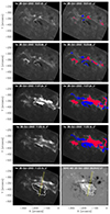 |
Fig. 1. Evolution of the 2003 October 28 flare observed by the USO Hα telescope for four different time steps covering the start, maximum, and decay phase of the flare (left panels). In the right panels, the total flare ribbon areas detected up to the respective recording time of the image are overplotted, separately in blue (red) for the positive (negative) magnetic polarities. In the bottom panels, we outline the flare PIL (white contour) derived from the corresponding pre-flare MDI LOS magnetic map shown in the right bottom panel. The narrow yellow rectangle in the bottom panels represents an example of one direction perpendicular to the local PIL segment (red line) along which the flare ribbons separation motion and Ec(r, t) were derived. |
Figure 2 plots the GOES 1−8 Å SXR flux along with the inferred time evolution of the reconnection fluxes derived during the flare impulsive phase, separately for the positive and negative magnetic fields. The reconnection flux φ(tk) is defined as the sum of all fluxes in the flare areas that brightened up until a given time, tk. Ideally, φ+ and φ− should be identical, as equal amounts of positive and negative magnetic flux participate in the reconnection. However, measurements do not always yield a perfect balance between the positive and negative fluxes (e.g., Fletcher & Hudson 2001). Given the uncertainties involved in the measurements, flares with R = φ+(t)/φ−(t) from 0.5 to 2.0 are generally regarded as showing a good flux balance (Qiu & Yurchyshyn 2005; Miklenic et al. 2009; Tschernitz et al. 2018). Figure 2a shows that our measurements obey this requirement.
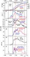 |
Fig. 2. Observables of the 2003 October 28 flare. (a) Reconnection flux derived in the positive (blue) and negative (red) domains (left Y-axis) and the GOES 1−8 Å soft X-ray flux ISXR(t) (black curve, right Y-axis). (b) Reconnection rates |

The total flare reconnection flux φ(t) is defined as the mean of the absolute values of the reconnection fluxes in both polarity regions at the end of the time series, that is,
 (4)
(4)
where φ+(t) and φ−(t) are the cumulated magnetic fluxes in the positive and negative polarity regions. The total amount of magnetic flux participating in the reconnection up to the time 11:13:30 UT was (14.8 ± 2.7)×1021 Mx. The magnetic-flux change rates  and
and  were calculated as the time derivative of the reconnected flux separately for each magnetic polarity. These rates are presented in Fig. 2b. The mismatch between these two values is largest during the rise phases (before the red line in Fig. 2), which might be associated with a greater inclination of the field in this early phase of the flare consistent with the lower altitude inferred for the X-point in Sect. 4.4.
  reached its absolute maximum equal to (4.6 ± 0.2)×1019 Mx s−1 at 11:02:35 UT.
  reached maximum at 11:03:41 UT with a lower value (3.7 ± 0.1)×1019 Mx s−1. Afterward, the reconnection rates declined but were still at a level ≥1 × 10¹⁹ Mx s−1 for at least 10 min, implying ongoing magnetic reconnection.
4.3. Energy release and high energy emissions
Figure 2c shows the temporal profile of the time derivative of the GOES 1−8 Å flux, İSXR(t), and the HXR emission at 15−40 keV registered by CORONAS-F/SPR-N and at 16−69 keV registered by Konus-Wind. Figure 2d shows time profiles of the nonthermal HXR emission at 40−100 keV from CORONAS-F/SPR-N and at 69−285 keV from Konus-Wind. CORONAS-F/SPR-N data are useful because the SPR-N detector had a small geometric factor and therefore it was not saturated during this intense flare. Figure 2e shows 15.4 GHz radio-emission from the RSTN. These data demonstrate that the Neupert effect (Neupert 1968; Veronig et al. 2002) revealed itself in the flare under consideration. Therefore, we hereafter use the GOES SXR derivative, İSXR(t), as a proxy of the flare energy release. Figure 2f shows HXR emission observed by the Anti-Coincidence Shield of SPI above 150 keV (Kiener et al. 2006) (red) and Konus-Wind rate at 285−1128 keV (blue).
Konus-Wind detected 16−69 keV HXR emission at the flare beginning simultaneously with the 15.4 GHz radio emission indicative of electron acceleration up to ≳100 keV when the reconnection rates  of both polarities have not yet exceeded (1 − 2)×1018 Mx s−1. We adopted the time T0 = 10:58:30 UT as the flare onset and divided the flare impulsive phase based on the
  , ISXR, İSXR and HXR time profiles as follows: the early rise phase: 10:58:30–11:01:16 UT (T0 − T1), the main rise phase: 11:01:16–11:03:40 UT (T1 − T2), the main energy release phase: 11:03:40–11:10:00 UT (T2 − T3). We adopted the time, T3, as the end of the main energy release phase. Thus, the main energy release phase began and continued to develop when the global reconnection rate has already gone over the maximum.
Figure 3 reproduced from Fig. 5 of Kuznetsov et al. (2011) presents the time profiles of high-energy emission measured by CORONAS-F/SONG in the wide energy channels from 225 keV up to 150 MeV. SONG observations of the flare began after CORONAS-F has left the outer radiation belt at 11:02 UT and covered most part of the main rise phase and the entire main energy release phase. Two vertical lines added in Fig. 3 indicate the beginning and the end of the main energy release phase: 11:03:40–11:10:00 UT (T2 − T3). Figures 2 and 3 show that particle acceleration/energy release happened as several separate episodes. As it is expected from the standard flare model, the reconnection rate variations agree with those of particle acceleration. Indeed, such a correspondence being in agreement with the model of Vršnak (2016) is seen in both the early rise and in the main rise phases. However, the main energy release began later, around ∼11:03:45 UT when the positive polarity reconnection rate reached its peak and the negative polarity one has already passed the maximum. The main energy release maximum was observed at ∼11:05:20±00:00:06 UT.
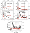 |
Fig. 3. Time evolution of CORONAS/SONG response during the flare of 28 October 2003 starting at 11:02:00 UT. The background count rates are subtracted. The left axis in each panel corresponds to the lower energy channel, the right axis to the higher energy one. Reproduced from Fig. 5 of Kuznetsov et al. (2011) under Springer Nature License Number # 5605391357254. |
4.4. Local electric field strength
To study the evolution of the local reconnection rates (coronal electric fields) Ec(r, t), we manually selected positions along the PIL, from where we track the flare ribbon separation motion. The PIL location was selected in such a way that the conjugate flare ribbons can be tracked simultaneously in a direction perpendicular to the PIL. The analysis is performed for 30 positions along the PIL and the different colors correspond to the selected tracking directions (see Fig. 4). Each rectangle perpendicular to the PIL indicates a sub-region (length of 200″ and width of 6″) used to track the ribbons. In the tracking, the outer front of the flare ribbons needs to be identified, because this part is related to the newly reconnected field lines along which the accelerated particles travel downwards to the solar surface. For a detailed description of the method and the uncertainties, we refer to Hinterreiter et al. (2018). We determine Ec(r, t) by tracking the ribbon position as a function of time and evaluating the underlying photospheric magnetic field strength. Then the Ec(r, t) value in each location was calculated using Eq. (1).
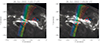 |
Fig. 4. Hα images observed at the main rise phase (left) and at the main energy release phase peak (right). The local PIL segment is shown by the white line. Multicolor rectangles indicate the directions perpendicular to the local PIL segments, along which we followed the flare ribbon separation to derive the local electric field strength evolution Ec(r, t). Overlaid on the Hα image is the RHESSI HXR 100−200 keV (blue) and the 2.2 MeV γ-ray line (red) contours for 11:06:20–11:09:20 UT (from Hurford et al. 2006). The two HXR FPs lie on the outer borders of the extended conjugated Hα ribbons. We note that one of the two footpoints (rooted in negative polarity) is located outside the 30 positions along the PIL that we are studying. |
In Fig. 4, we also overplot the contours of the 100−200 keV bremsstrahlung and the 2.2 MeV γ-ray line emission sources reconstructed from RHESSI observations in Hurford et al. (2006). These images were obtained after the spacecraft came out of the Earth shadow at 11:06:43 UT. Two footpoints (FPs) are observed in HXRs (electron bremsstrahlung) positioned on localized regions at the outer borders of the extended conjugate Hα ribbons. We restricted the analysis up to the time 11:08:00 UT when considering the Ec(r, t) time evolution.
Figure 5 shows contour plots of Ec(r, t) at each position number versus time in the positive (P) and negative (N) polarities derived for 30 positions during the flare impulsive phase. The evolution of the Ec(r, t) at the different ribbon locations reflects the propagation of magnetic reconnection along the arcade of the conjugate loops rooted in positive and negative polarities. The Ec(r, t) distributions look slightly different in the two polarities. This is because a slit in a given direction across the local PIL used to derive the Ec profiles, does not necessarily cover the conjugated FPs in both polarities, because the overall flare loop (and ribbon) system is highly sheared. We found that:
-
In the positive polarity domain, the highest electric field strength Ec, max ≈ 125 V cm−1. Values ≥95% of Ec, max were observed between 11:03:10 and 11:03:40 UT in position numbers P4–P6.
-
In the negative polarity domain, we obtain Ec, max ≈ 80 V cm−1, and values ≥95% of Ec, max were observed at position numbers N14–N16 at the same time as for the positive polarity.
-
Ec(r, t) of both polarities starts to fall off around 11:03:20–11:03:40 UT, namely, around T2 at the main flare energy release onset.
-
Afterwards, the peak Ec(r, t) of the negative polarity was observed around N11 position with a 1 min delay relative to T2 (see Fig. 6b). A similar peak in the positive polarity was less pronounced as it merged with the main peak.
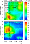 |
Fig. 5. Spatio-temporal map of the coronal electric field strengths Ec(r, t). (a) Positive polarity contour plot. The shaded area marks the region in which the electric field could not be determined; (b) Negative polarity contour plot. The dashed vertical line indicates hereinafter T2 = 11:03:40 UT. |
The Ec(r, t) evolution at the P4–P6 and N15–N16 positions are shown in Figs. 6a and b. According to the standard model of solar flares, a pair of flare FPs in the chromosphere maps the reconnected magnetic field lines in the current sheet, whose apex runs close to the “X-point”. We adopted positions P4 and N16 as most representative ones. The Pearson correlation coefficient between Ec(r, t) in these positions is r = 0.95, indicative of a magnetic connectivity between them.
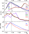 |
Fig. 6. Evolution of the coronal electric field Ec(r, t) in selected positions of positive (a) and negative (b) magnetic polarities. (c) Comparison of the Ec(r, t) evolution in positions P4 and N16 (cf. Fig. 4). |
We calculated the distance between the outer fronts of the Hα ribbons located in the P4 and N16 positions and the shear angle between them. The P4 position crosses the PIL at x = −156″, y = −357″, the N16 position crosses the PIL at x = −140″, y = −360″. Assuming a semicircle shape of the loop connecting these FPs, we estimated the height of the reconnection X-point at each time step (Fig. 7a). A cartoon of the time evolution of this loop seen at a side view is presented in Fig. 7d. The derived height of the X-point was ∼8−12 Mm in the main rise flare phase showings a slow rise (v ∼ 20 km s−1). Around T2, it began to ascend faster (v ∼ 60 km s−1). Figure 7b shows the evolution of the shear angle derived from P4 and N16 positions, whereas Fig. 7c shows the evolution of the shear angle derived from the observations of the EUV strongest brightening pairs (from Fig. 10 of Su et al. 2006). It is seen that the shear angles decrease during the main rise phase. The change of the velocity of X-point ascent and the change in shear angle occurred roughly simultaneously around 11:03−11:04 UT, namely, close to T2 = 11:03:40 UT.
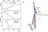 |
Fig. 7. Evolving morphology of the magnetic reconnection. (a) Evolution of the height of the reconnection X-point derived from the loop connecting positions P4 and N16. (b) Shear angle derived from the Ec evolution of positions P4 and N16. (c) Shear angle derived from EUV observations (from Fig. 10 of Su et al. 2006). (d) Axonometric projection cartoon of the time evolution of the presumable loop connecting positions P4 and N16 (side view). |
4.5. High-energy X-ray and γ-ray emission spectra
In this section, we present and discuss the observations of the flare high-energy emission, the results of Konus-Wind spectral analysis along with published INTEGRAL/SPI and CORONAS/SONG spectra.
4.5.1. The early flare phase and the main rise phase
To specify the γ-ray emission components and the spectral characteristics, we used Konus-Wind data. A detailed description of the Konus-Wind data, response files and spectra deconvolution can be found in Lysenko et al. (2022). Energy spectra were accumulated in the energy range ∼0.35−15 MeV (60 channels). The accumulation of multichannel spectra starts with the Konus-Wind trigger time 11:01:12 UT (corrected for the light propagation to the Earth) and ended at 11:02:57 UT. The γ-ray spectra were fitted using the XSPEC package (Arnaud 1996) with the following components. The continuum was described by the sum of two components: (i) the power-law (PL), and (ii) the power-law with an exponential cutoff at higher energies (CPL). De-excitation γ-ray lines were fitted with the template proposed by Murphy et al. (2009). Electron-positron annihilation and neutron-capture lines were fitted by gaussians with fixed positions at 511 keV and 2223 keV and fixed σ at 5 keV and 0.1 keV, respectively.
In Fig. 8, we present Konus-Wind spectra accumulated subsequently during the main rise phase of the flare6. This spectral analysis shows:
-
A line-free, very soft electron bremsstrahlung component consistent with the PL model with a spectral index of ∼5 during the time interval 11:01:12–11:01:49 UT (not shown in the figure).
-
The appearance of emission above 1 MeV at 11:01:49 UT, related to the hard continuum component described by the CPL model (Fig. 8, left).
-
The appearance of γ-ray lines, including de-excitation lines, electron-positron annihilation line, and neutron capture line resulting from nuclear interactions of accelerated ions in the solar atmosphere at 11:02:16 UT (Fig. 8, middle).
-
The CPL continuum exceeds 14 MeV during time interval 11:02:40–11:02:48 UT (Fig. 8, right), which coincides with the time of the first maximum of CORONAS-F/SONG observations in the 40–60 MeV energy range at 11:02:36–11:02:48 UT (see Fig. 3).
-
γ-ray lines are barely seen above the continuum. This is consistent with the results of the high-resolution γ-ray spectrometer INTEGRAL/SPI. Due to the exceptional intensity of bremsstrahlung, INTEGRAL/SPI distinguished only two narrow γ-ray lines in the 600 keV–8 MeV energy range, namely at 2.223 MeV and 4.4 MeV.
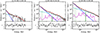 |
Fig. 8. Konus-Wind spectra accumulated over three time intervals during the main rise phase: 11:01:49–11:02:16 (left), 11:02:16–11:02:32 (middle), 11:02:40–11:02:48 (right). Black crosses represent the photon spectrum, color curves indicate model components: PL (blue), CPL (cian), nuclear deexcitation lines (magenta), neutron capture line (green), electron-positron annihilation line (dashed green), and the sum of all components (red). The bottom panels on each plot represent the fit residuals. |
In the following, we put these findings into context with the SONG spectral analysis in Kuznetsov et al. (2011). SONG had 12 broad energy channels and did not resolve discrete narrow γ-ray lines, including the neutron-capture line at 2.223 MeV. The top panel of Fig. 9 shows the spectrum accumulated over the main rise phase; the bottom panel shows the spectrum accumulated in the main energy release phase. Kuznetsov et al. (2011) adopted a two-component model: an electron bremsstrahlung component described by a power-law above 1 MeV with an index gradually changing with energy or as an exponential high-energy cutoff; the second component, π-decay emission, having a broad “line” due to neutral-pion decay, peaking at 67 MeV, plus a continuum due to bremsstrahlung from electrons and positrons produced in charged pion decay (Murphy et al. 1987). Kuznetsov et al. (2011) emphasized that they did not explicitly take into account the contribution of the γ-ray lines, as they have focused on the π-decay component; this would overestimate the continuum if a significant γ-ray line contribution were present. Kuznetsov et al. (2011) also performed a similar fit using channels above 10 MeV, that is, explicitly avoiding those lines. The results of both fittings showed that neglecting the contribution of γ-ray lines did not change the resulting π-decay flux. The fits of Konus-Wind spectra obtained with higher spectral resolution confirm that the γ-ray line contribution were weak, which justifies its omission by Kuznetsov et al. (2011). Therefore, the SONG fit showed that the primary electrons were accelerated at least up to 22.5−40 MeV and that the estimated upper limit of the π-decay emission is ≤5 × 10⁻⁴ phot cm−2 s−1 MeV−1 at 100 MeV.
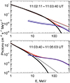 |
Fig. 9. Gamma-ray emission spectra observed by CORONAS/SONG; from Fig. 8 of Kuznetsov et al. (2011), reproduced under Springer Nature License Number # 5605391357254. Upper panel: spectrum accumulated over the main rise phase. Bottom panel: spectrum accumulated over the most part of the main energy release phase. The red curves represent the total spectra and the black curves indicate the continuum component (thin curves correspond to a power law with varying index and the thick curves correspond to a power law with an exponential cutoff), while the blue curves show the π-decay component. |
4.5.2. The main energy release phase
This flare phase lasted ∼6 min (11:03:40−11:10:00 UT) (see Figs. 2 and 3). The accumulation of Konus multichannel spectra terminated at 11:02:57 UT. We used results of INTEGRAL/SPI and GORONAS-F/SONG spectral analysis of this phase. Kiener et al. (2006) found clear evidence of the bremsstrahlung continuum softening and the increase of the γ-ray line intensity in this phase (see their Table 2). The SONG γ-ray spectrum in the time interval between 11:03:40−11:05:03 UT (bottom panel of Fig. 9) shows that the continuum became negligible compared to the π-decay component at energies > 22.5 MeV. An important point is that the count rate of the high energy SONG channels, > 90 MeV (Fig. 3), which was obviously due to the π-decay emission, had emerged around the main flare energy release beginning at T2 = 11:03:40 UT. Kuznetsov et al. (2011) followed the time evolution of the π-decay emission until 11:10:20−11:12:20 UT. This component reached its maximum of (1.1 ± 0.1)×10−2 phot cm−2 s−1 MeV−1 at 11:03:40−11:05:03 UT (see the bottom panel of Fig. 9), simultaneously with the maximum of the flare energy release.
4.5.3. Constraints on the accelerated ion spectrum
The spectral hardness of the accelerated ions can be found through comparison of fluxes or fluences of different components of the γ-ray emission: the neutron-capture line 2.223 MeV, F2.2, the prompt 4.4 MeV 12C*, and 6.1 MeV 16O* nuclear de-excitation lines, and the pion-decay component, Fπ. The pion production cross section has a very small value near the threshold of this reaction of 200−300 MeV, and increases by a factor of 100 when the energy of accelerated protons doubles. Thus, for hard spectra, the relevant ion energy range extends from a few MeV nucl−1 up to > 100 MeV nucl−1. For soft spectra, the relevant ion energy range is much narrower, from less than 1 to a few MeV nucl−1 (see Murphy et al. 2007).
The primary accelerated ions are assumed to have a power-law energy distribution with spectral index S. Tatischeff et al. (2005) deduced the spectral index S for this event from the 2.223 MeV to the 4.4 and 6.1 MeV line fluence ratios from the INTEGRAL/SPI data in the range 3 ≤ S ≤ 4. Share et al. (2004) found S close to 3.4 for this flare after 11:06 UT from RHESSI data. Kuznetsov et al. (2011) combined the CORONAS/SONG Fπ fluxes with the nuclear deexcitation line flux in the 4−7 MeV range, F4 − 7, obtained from INTEGRAL/SPI data by Kiener et al. (2006) and derived the hardest spectrum with S = 2.8 ± 0.1 near the peak of the π-decay emission and S = 3.1 ± 0.1 afterward. In summary, these findings show that the power law index of the proton spectrum is S ∼ 3 over a wide energy range from several MeV to several hundred MeV. In comparison with other strong flares, Omodei et al. (2018) found the hardest value S = 3.2 ± 0.1 during the main energy release phase of the X8.2 2017 September 10 flare (at 15:57:55−15:58:54 UT).
5. Association of the reconnection rates with the high-energy particle acceleration
Figure 10 shows the evolution of the reconnection rates together with various manifestations of high-energy electrons and protons. Panel a shows the distribution of the negative polarity electric field Ec(r, t) at various positions relative to the PIL over time, along with the derived increase of the X-point height (right axes). Panel b shows the time evolution of the global reconnection rates of the negative and positive polarity. Panel c shows the bremsstrahlung observed by the Anti-Coincidence Shield of SPI above 150 keV (Kiener et al. 2006), and of 285−1128 keV observed by Konus-Wind. Panel d shows the prompt 4.4 and 6.1 MeV γ-ray line profile (from Kiener et al. 2006). The count rates of the two CORONAS-F/SONG channels at 40−60 MeV and 60−90 MeV are shown in panels e, f. We can see that time T2 = 11:03:40 UT identified as the onset of the main energy release phase (see Sect. 4.3) demarcates two time intervals with different signatures of charged particle acceleration.
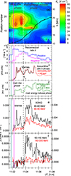 |
Fig. 10. Local and global reconnection rates collated with high-energy electron and proton emissions during the main rise phase and the main energy release phase of the 2003 October 28 flare. (a) Contour plot of the local reconnection rate Ec(t) in the negative polarity domain, overplotted with the derived height-time evolution of the X-point (black points, right axis). (b) Time profiles of the global reconnection rates |

The hard bremsstrahlung component, which is usually described by a CPL model, appeared in the flare spectrum in the time interval 11:01:49−11:02:16 UT during the main rise phase. At that time, the local reconnection rate in the negative polarity reached Ec ≈ 60 V cm−1 and the averaged global reconnection rate  Mx s−1. Prompt γ-ray line emission appeared later at 11:02:16 UT, where the reconnection rates reached values of Ec ≈ 75 V cm−1 and
  Mx s−1. In the main rise phase, two maxima of the bremsstrahlung and γ-ray line emission occurred simultaneously (within the available time resolution) at 11:02:40 UT and at 11:03:12 UT. Putting this all together, it is tempting to associate the electron and proton acceleration peaks with the above two maxima of Ec (see also Fig. 5), which in turn were associated with regions of the reconstructed X-point height h ≈ 10 − 12 Mm.
The time interval between 11:03:45 and 11:10:00 UT corresponds to the flare main energy release. It is important that the temporal profiles of the global reconnection rates in both polarities,  and
and  , decreased after ∼11:03:45 UT (see Fig. 10b). The beginning of a new process of the electron acceleration was identified based on the Konus-Wind 285−1128 keV data at 11:03:45 (Fig. 10c). A new increase of γ-ray line flux observed by the INTEGRAL/SPI with a 15 s time sequence occurred in the time interval 11:03:42−11:03:57 UT giving a good agreement with the electron acceleration onset time. Spectral analysis of SONG data (Kuznetsov et al. 2011) showed that the count rates of the SONG channels > 60 MeV are entirely due to π-decay emission in the time interval 11:03:47−11:04:15 UT and afterward. Moreover, Fig. 3 shows that statistically significant π-decay emission appeared promptly during one bin of SONG time resolution (4 s) at 11:03:49 UT ± 2 s.
The π-decay emission jumped promptly up to 0.75 Imax with a time lag of 9 ± 2 s relative to the electron acceleration onset. Apparently, this delay provides evidence that protons need a few extra seconds to gain enough energy to create the observable number of photons. Above, we define the main energy release phase of the flare based on the electron acceleration as a proxy (see Fig. 2). We have now shown that this is also a “high-energy release” phase, when the most efficient acceleration of protons to very high energies occurred. The height of the X-point during this energy release phase is h ∼ 15 − 20 Mm.
The new acceleration process described above begins when the contours of Ec have been reshaped and the implied X-point has just moved up. Although there are no direct observations of the flare morphology in the corona in the 2003 October 28 flare available (as the event occurred on the solar disk), we suggest an evolving morphology similar to that reported for the well-observed 2017 September 10 X8 limb flare (Gary et al. 2018; Veronig et al. 2018; Fleishman et al. 2020; Chen et al. 2020; Li et al. 2022; Kong et al. 2022). We propose that over the course of the flare, two distinct sources of accelerated particles were sequentially formed, initially one at a height h ∼ 10 − 12 Mm and then the other at h ∼ 15 − 20 Mm. We attribute these regions to the cusp location and to the bottom of the reconnection current sheet. We have demonstrated that the flare main energy release and proton acceleration up to subrelativistic energies began just when the reconnection rate was going through its maximum, namely, after a major change in the topology of the flare, when the erupting flux rope is already far away from the flare site.
6. Summary and discussion
We have investigated the impulsive phase of the X17.2 eruptive flare of 2003 October 28 to reveal links in the chain of the evolution of the energy release as quantified by the magnetic reconnection rates and of the acceleration of electrons and protons to high energies. Our main findings are:
-
The distinct phases of the energy release, namely, the rise phase and the main energy release phase, are morphologically different from each other and are also different in terms of their associated signatures of the particle acceleration.
-
The rise phase is associated with a larger reconnection rate (stronger coronal electric field) and relatively low positions of the implied reconnection X-point as derived from the conjugate flare ribbon locations. This phase demonstrates very efficient acceleration of nonthermal electrons and protons up to dozens of MeV, which is confirmed by detection of electron bremsstrahlung up to ∼40−60 MeV and the simultaneous γ-ray de-excitation lines. The relatively low position of the implied reconnection X-point is analogous to the results obtained by Kurt et al. (1996, 2000), who proposed that a low height of the acceleration region could be favorable for electron acceleration up to ∼100 MeV.
-
The main energy release flare phase occurring later is associated with a higher location of the reconnection X-point. At this stage, protons are accelerated to higher energies (> 200 MeV), while electrons are accelerated to lower energies (< 20 MeV).
Similar relationships between the reconnection rates and particle acceleration properties at the rise and main flare phases have been noted for some other cases (e.g., Share et al. 2022; Yushkov et al. 2023) with the π-decay gamma-ray component observed in the impulsive flare phase, which can imply a fundamental character of the reported relationships for the understanding of the solar flare process.
We are curious to extend the discussion to the questions of why: (1) at the rise phase, the electrons are accelerated up to dozens (or even one hundred) of MeV, while protons not, and (2) at the following main energy release phase, the protons are accelerated to hundreds of MeV, while the electrons are accelerated only up to much smaller energies than at the rise phase. A possible reason for that could be the evolving relationships between three characteristic time scales: the acceleration rate, Tacc (the energy e-folding time scale), the energy loss rate, Tloss, and the residence time, Tres, of the particles in the acceleration region. Particles can be accelerated to a given energy, E, if the acceleration up to this energy occurs faster than the energy loss at this energy. Thus, the highest energy, Emax, is defined from the equality of Tacc(Emax) = Tloss(Emax), provided that the energy loss timescale is shorter than the residence time. In the opposite case, the highest energy of the accelerated particle is defined by another equality, Tacc(Emax) = Tres(Emax). One important difference between electrons and protons (nuclei) are their highly different mechanisms of the energy loss due to large differences in their masses. For highly relativistic electrons, the main energy-loss mechanism in the magnetized coronal plasma is the synchrotron energy losses with the characteristic time scale (in seconds):
 (5)
(5)
where B is the magnetic field in G and γ = E/mc2 is the Lorentz factor; see Eq. (12.52) in Fleishman & Toptygin (2013). This loss is negligible for protons and other nuclei. We propose that the acceleration rate of the electrons is largest at the rise phase, when the measured reconnection rate is highest, which would permit the electrons to be accelerated to rather high energies of the order of 100 MeV. At this stage, the flare undergoes a fast evolution, which implies that the acceleration region may evolve quickly as well (i.e., moving up following the reconnection process). This means that the protons might not reside in the acceleration region long enough to be accelerated to energies higher than ∼100 MeV.
Subsequently, at the main energy release phase, the reconnection rate decreases, which can imply that the acceleration efficiency decreases proportionally. This means that the maximum energy of the accelerated electrons also decreases to obey the new balance between the acceleration and loss rates, while the electrons that had accelerated earlier will lose their energy over several seconds according to Eq. (5) if the magnetic field in the acceleration region is about 1 kG (Fleishman et al. 2020). However, if the particles can now reside longer in the acceleration region, for instance, due to efficient particle trapping by high levels of turbulence, protons can gain much higher energies than at the rise phase. Another factor that can support ion acceleration to high energies is the decrease of the guiding magnetic field (Arnold et al. 2021; Dahlin et al. 2022) due to the eruption of a flux rope, which is far away from the acceleration region at this stage of the flare.
This reasoning is consistent with microwave imaging observations of the powerful X8 flare on 2017 September 10 that was observed on the limb; following the eruption and the restructuring of the magnetic connectivity, the acceleration site located within the cusp region revealed highly efficient trapping of the nonthermal particles at the main flare phase (Fleishman et al. 2022). This was presumably due to enhanced levels of turbulence. The particles reside several minutes in the acceleration region, which, in the case of protons and other ions, can permit their acceleration to rather high energies sufficient to produce the π-decay gamma-ray component.
At the time of the flare, Konus-Wind was ∼3.25 light seconds farther from the Sun than the Earth, thus, for the comparison to the CORONAS/SONG results fluxes obtained by Konus-Wind have to be multiplied by a factor of ∼1.014. As this value lies within uncertanties we did not correct photon fluxes in Fig. 8 to account for the distance difference.
Acknowledgments
We thank Dr. V. Bogomolov for the kindly provided CORONAS-F/SPRN data. We thank Kiener et al. for providing the data of INTEGRAL/SPI. A.M.V. acknowledges the Austrian Science Fund (FWF) 10.55776/I4555. This work was supported in part by NSF grant AGS-2121632, and NASA grants 80NSSC20K0718 and 80NSSC23K0090 to New Jersey Institute of Technology (GDF). The work of ALL was supported by the basic funding program of the Ioffe Institute No. FFUG-2024-0002.
References
- Aptekar, R. L., Frederiks, D. D., Golenetskii, S. V., et al. 1995, Space Sci. Rev., 71, 265 [NASA ADS] [CrossRef] [Google Scholar]
- Arnaud, K. A. 1996, in Astronomical Data Analysis Software and Systems V, eds. G. H. Jacoby, & J. Barnes, ASP Conf. Ser., 101, 17 [NASA ADS] [Google Scholar]
- Arnold, H., Drake, J. F., Swisdak, M., et al. 2021, Phys. Rev. Lett., 126, 135101 [NASA ADS] [CrossRef] [Google Scholar]
- Asai, A., Yokoyama, T., Shimojo, M., et al. 2004, ApJ, 611, 557 [NASA ADS] [CrossRef] [Google Scholar]
- Aschwanden, M. J., Caspi, A., Cohen, C. M. S., et al. 2017, ApJ, 836, 17 [Google Scholar]
- Bastian, T. S., Benz, A. O., & Gary, D. E. 1998, ARA&A, 36, 131 [Google Scholar]
- Benz, A. O. 2017, Liv. Rev. Sol. Phys., 14, 2 [Google Scholar]
- Bieber, J. W., Clem, J., Evenson, P., et al. 2005, Geophys. Res. Lett., 32, L03S02 [NASA ADS] [CrossRef] [Google Scholar]
- Carmichael, H. 1964, NASA Spec. Publ., 50, 451 [NASA ADS] [Google Scholar]
- Caspi, A., & Lin, R. P. 2010, ApJ, 725, L161 [CrossRef] [Google Scholar]
- Caspi, A., Krucker, S., Lin, R. P., et al. 2014, ApJ, 781, 43 [NASA ADS] [CrossRef] [Google Scholar]
- Chen, B., Shen, C., Gary, D. E., et al. 2020, Nat. Astron., 4, 1140 [Google Scholar]
- Chen, B., Battaglia, M., Krucker, S., Reeves, K. K., & Glesener, L. 2021, ApJ, 908, L55 [CrossRef] [Google Scholar]
- Dahlin, J. T., Antiochos, S. K., Qiu, J., & DeVore, C. R. 2022, ApJ, 932, 94 [CrossRef] [Google Scholar]
- Dennis, B. R., & Zarro, D. M. 1993, Sol. Phys., 146, 177 [CrossRef] [Google Scholar]
- Dennis, B. R., Veronig, A., Schwartz, R. A., et al. 2003, Adv. Space Res., 32, 2459 [NASA ADS] [Google Scholar]
- Dermer, C. D., & Ramaty, R. 1986, ApJ, 301, 962 [CrossRef] [Google Scholar]
- Emslie, A. G., Dennis, B. R., Shih, A. Y., et al. 2012, ApJ, 759, 71 [Google Scholar]
- Fedenev, V. V., Anfinogentov, S. A., & Fleishman, G. D. 2023, ApJ, 943, 160 [NASA ADS] [CrossRef] [Google Scholar]
- Fleishman, G. D., & Toptygin, I. N. 2013, Cosmic Electrodynamics: Electrodynamics and Magnetic Hydrodynamics of Cosmic Plasmas (New York: Springer), 388 [Google Scholar]
- Fleishman, G. D., Kontar, E. P., Nita, G. M., & Gary, D. E. 2011, ApJ, 731, L19 [NASA ADS] [CrossRef] [Google Scholar]
- Fleishman, G. D., Nita, G. M., Gary, D. E., et al. 2015, ApJ, 802, 122 [CrossRef] [Google Scholar]
- Fleishman, G. D., Nita, G. M., Kontar, E. P., & Gary, D. E. 2016, ApJ, 826, 38 [NASA ADS] [CrossRef] [Google Scholar]
- Fleishman, G. D., Gary, D. E., Chen, B., et al. 2020, Science, 367, 278 [NASA ADS] [CrossRef] [Google Scholar]
- Fleishman, G. D., Nita, G. M., Chen, B., Yu, S., & Gary, D. E. 2022, Nature, 606, 674 [NASA ADS] [CrossRef] [Google Scholar]
- Fletcher, L., & Hudson, H. 2001, Sol. Phys., 204, 69 [CrossRef] [Google Scholar]
- Fletcher, L., Dennis, B. R., Hudson, H. S., et al. 2011, Space Sci. Rev., 159, 19 [Google Scholar]
- Forbes, T. G., & Lin, J. 2000, J. Atmos. Solar-Terr. Phys., 62, 1499 [NASA ADS] [CrossRef] [Google Scholar]
- Forbes, T. G., & Priest, E. R. 1984, Sol. Phys., 94, 315 [NASA ADS] [CrossRef] [Google Scholar]
- Gary, D. E., & Hurford, G. J. 1989, ApJ, 339, 1115 [NASA ADS] [CrossRef] [Google Scholar]
- Gary, D. E., Chen, B., Dennis, B. R., et al. 2018, ApJ, 863, 83 [CrossRef] [Google Scholar]
- Hinterreiter, J., Veronig, A. M., Thalmann, J. K., Tschernitz, J., & Pötzi, W. 2018, Sol. Phys., 293, 38 [NASA ADS] [CrossRef] [Google Scholar]
- Hirayama, T. 1974, Sol. Phys., 34, 323 [Google Scholar]
- Holman, G. D. 2016, J. Geophys. Res.: Space Phys., 121, 11,667 [NASA ADS] [CrossRef] [Google Scholar]
- Holman, G. D., Aschwanden, M. J., Aurass, H., et al. 2011, Space Sci. Rev., 159, 107 [NASA ADS] [CrossRef] [Google Scholar]
- Hudson, H. S. 1991, Sol. Phys., 133, 357 [Google Scholar]
- Hudson, H., Cliver, E., White, S., et al. 2024, Sol. Phys., 299, 39 [NASA ADS] [CrossRef] [Google Scholar]
- Hurford, G. J., Krucker, S., Lin, R. P., et al. 2006, ApJ, 644, L93 [Google Scholar]
- Jing, J., Qiu, J., Lin, J., et al. 2005, ApJ, 620, 1085 [NASA ADS] [CrossRef] [Google Scholar]
- Jokipii, J. R. 1979, in Particle Acceleration Mechanisms in Astrophysics, eds. J. Arons, C. McKee, & C. Max, AIP Conf. Ser., 56, 1 [NASA ADS] [CrossRef] [Google Scholar]
- Kazachenko, M. D., Lynch, B. J., Welsch, B. T., & Sun, X. 2017, ApJ, 845, 49 [NASA ADS] [CrossRef] [Google Scholar]
- Kiener, J., Gros, M., Tatischeff, V., & Weidenspointner, G. 2006, A&A, 445, 725 [NASA ADS] [CrossRef] [EDP Sciences] [Google Scholar]
- Kong, X., Ye, J., Chen, B., et al. 2022, ApJ, 933, 93 [NASA ADS] [CrossRef] [Google Scholar]
- Kontar, E. P., Brown, J. C., Emslie, A. G., et al. 2011, Space Sci. Rev., 159, 301 [NASA ADS] [CrossRef] [Google Scholar]
- Kontar, E. P., Perez, J. E., Harra, L. K., et al. 2017, Phys. Rev. Lett., 118, 155101 [NASA ADS] [CrossRef] [Google Scholar]
- Kopp, R. A., & Pneuman, G. W. 1976, Sol. Phys., 50, 85 [Google Scholar]
- Krucker, S., Fivian, M. D., & Lin, R. P. 2005, Adv. Space Res., 35, 1707 [NASA ADS] [CrossRef] [Google Scholar]
- Krucker, S., Hudson, H. S., Glesener, L., et al. 2010, ApJ, 714, 1108 [NASA ADS] [CrossRef] [Google Scholar]
- Krucker, S., Hudson, H. S., Jeffrey, N. L. S., et al. 2011, ApJ, 739, 96 [NASA ADS] [CrossRef] [Google Scholar]
- Kurt, V., Akimov, V. V., & Leikov, N. G. 1996, in High Energy Solar Physics, eds. R. Ramaty, N. Mandzhavidze, & X. M. Hua, AIP Conf. Ser., 374, 237 [NASA ADS] [CrossRef] [Google Scholar]
- Kurt, V. G., Akimov, V. V., Hagyard, M. J., & Hathaway, D. H. 2000, in High Energy Solar Physics Workshop – Anticipating Hess!, eds. R. Ramaty, & N. Mandzhavidze, ASP Conf. Ser., 206, 426 [NASA ADS] [Google Scholar]
- Kuznetsov, S. N., Kurt, V. G., Yushkov, B. Y., Kudela, K., & Galkin, V. I. 2011, Sol. Phys., 268, 175 [NASA ADS] [CrossRef] [Google Scholar]
- Li, T., Priest, E., & Guo, R. 2021, Proc. R. Soc. London Ser. A, 477, 20200949 [NASA ADS] [Google Scholar]
- Li, X., Guo, F., Chen, B., Shen, C., & Glesener, L. 2022, ApJ, 932, 92 [CrossRef] [Google Scholar]
- Lingenfelter, R. E. 1969, Sol. Phys., 8, 341 [NASA ADS] [CrossRef] [Google Scholar]
- Lingenfelter, R. E., & Ramaty, R. 1967, High-Energy Nuclear Reactions in Astrophysics (New York: Benjamin), 99 [Google Scholar]
- Litvinenko, Y. E., & Somov, B. V. 1995, Sol. Phys., 158, 317 [NASA ADS] [Google Scholar]
- Liu, C., & Wang, H. 2009, ApJ, 696, L27 [NASA ADS] [CrossRef] [Google Scholar]
- Liu, W., Chen, Q., & Petrosian, V. 2013, ApJ, 767, 168 [NASA ADS] [CrossRef] [Google Scholar]
- Livingston, W., Harvey, J. W., Malanushenko, O. V., & Webster, L. 2006, Sol. Phys., 239, 41 [NASA ADS] [CrossRef] [Google Scholar]
- Lysenko, A. L., Ulanov, M. V., Kuznetsov, A. A., et al. 2022, ApJS, 262, 32 [NASA ADS] [CrossRef] [Google Scholar]
- Martens, P. C. H., & Young, A. 1990, ApJS, 73, 333 [NASA ADS] [CrossRef] [Google Scholar]
- Masuda, S., Kosugi, T., Hara, H., Tsuneta, S., & Ogawara, Y. 1994, Nature, 371, 495 [CrossRef] [Google Scholar]
- Metcalf, T. R., Leka, K. D., & Mickey, D. L. 2005, ApJ, 623, L53 [NASA ADS] [CrossRef] [Google Scholar]
- Miklenic, C. H., Veronig, A. M., Vršnak, B., & Hanslmeier, A. 2007, A&A, 461, 697 [NASA ADS] [CrossRef] [EDP Sciences] [Google Scholar]
- Miklenic, C. H., Veronig, A. M., & Vršnak, B. 2009, A&A, 499, 893 [NASA ADS] [CrossRef] [EDP Sciences] [Google Scholar]
- Miller, J. A., & Ramaty, R. 1989, ApJ, 344, 973 [NASA ADS] [CrossRef] [Google Scholar]
- Miller, J. A., Cargill, P. J., Emslie, A. G., et al. 1997, J. Geophys. Res., 102, 14631 [NASA ADS] [CrossRef] [Google Scholar]
- Murphy, R. J., & Ramaty, R. 1984, Adv. Space Res., 4, 127 [NASA ADS] [CrossRef] [Google Scholar]
- Murphy, R. J., Dermer, C. D., & Ramaty, R. 1987, ApJS, 63, 721 [NASA ADS] [CrossRef] [Google Scholar]
- Murphy, R. J., Kozlovsky, B., Share, G. H., Hua, X. M., & Lingenfelter, R. E. 2007, ApJS, 168, 167 [CrossRef] [Google Scholar]
- Murphy, R. J., Kozlovsky, B., Kiener, J., & Share, G. H. 2009, ApJS, 183, 142 [NASA ADS] [CrossRef] [Google Scholar]
- Naus, S. J., Qiu, J., DeVore, C. R., et al. 2022, ApJ, 926, 218 [CrossRef] [Google Scholar]
- Neupert, W. M. 1968, ApJ, 153, L59 [NASA ADS] [CrossRef] [Google Scholar]
- Omodei, N., Pesce-Rollins, M., Longo, F., Allafort, A., & Krucker, S. 2018, ApJ, 865, L7 [NASA ADS] [CrossRef] [Google Scholar]
- Petrie, G. J. D. 2019, ApJS, 240, 11 [NASA ADS] [CrossRef] [Google Scholar]
- Petrosian, V. 2012, Space Sci. Rev., 173, 535 [NASA ADS] [CrossRef] [Google Scholar]
- Plainaki, C., Belov, A., Eroshenko, E., et al. 2005, Adv. Space Res., 35, 691 [CrossRef] [Google Scholar]
- Pötzi, W., Veronig, A. M., Riegler, G., et al. 2015, Sol. Phys., 290, 951 [Google Scholar]
- Priest, E., & Forbes, T. 2000, Magnetic Reconnection (Cambridge: Cambridge University Press) [CrossRef] [Google Scholar]
- Qiu, J. 2009, ApJ, 692, 1110 [NASA ADS] [CrossRef] [Google Scholar]
- Qiu, J., & Yurchyshyn, V. B. 2005, ApJ, 634, L121 [NASA ADS] [CrossRef] [Google Scholar]
- Qiu, J., Lee, J., Gary, D. E., & Wang, H. 2002, ApJ, 565, 1335 [NASA ADS] [CrossRef] [Google Scholar]
- Qiu, J., Wang, H., Cheng, C. Z., & Gary, D. E. 2004, ApJ, 604, 900 [NASA ADS] [CrossRef] [Google Scholar]
- Qiu, J., Liu, W., Hill, N., & Kazachenko, M. 2010, ApJ, 725, 319 [NASA ADS] [CrossRef] [Google Scholar]
- Ramaty, R., & Murphy, R. J. 1987, Space Sci. Rev., 45, 213 [NASA ADS] [CrossRef] [Google Scholar]
- Ramaty, R., Mandzhavidze, N., Kozlovsky, B., & Skibo, J. G. 1993, Adv. Space Res., 13, 275 [NASA ADS] [CrossRef] [Google Scholar]
- Scherrer, P. H., Bogart, R. S., Bush, R. I., et al. 1995, Sol. Phys., 162, 129 [Google Scholar]
- Share, G. H., Murphy, R. J., Smith, D. M., Schwartz, R. A., & Lin, R. P. 2004, ApJ, 615, L169 [NASA ADS] [CrossRef] [Google Scholar]
- Share, G. H., Murphy, R., Grove, J. E., & Shih, A. Y. 2022, AGU Fall Meet. Abstr., 2022, SH43A–03 [Google Scholar]
- Somov, B. V. 2013, Plasma Astrophysics, Part II (New York: Springer Science+Business Media), 392 [CrossRef] [Google Scholar]
- Sturrock, P. A. 1966, Nature, 211, 695 [Google Scholar]
- Su, Y. N., Golub, L., van Ballegooijen, A. A., & Gros, M. 2006, Sol. Phys., 236, 325 [NASA ADS] [CrossRef] [Google Scholar]
- Su, Y., Veronig, A. M., Holman, G. D., et al. 2013, Nat. Phys., 9, 489 [Google Scholar]
- Sui, L., Holman, G. D., & Dennis, B. R. 2004, ApJ, 612, 546 [NASA ADS] [CrossRef] [Google Scholar]
- Tatischeff, V., Kiener, J., & Gros, M. 2005, arXiv e-prints [arXiv:astro-ph/0501121] [Google Scholar]
- Temmer, M., Veronig, A. M., Vršnak, B., & Miklenic, C. 2007, ApJ, 654, 665 [NASA ADS] [CrossRef] [Google Scholar]
- Toriumi, S., & Wang, H. 2019, Liv. Rev. Sol. Phys., 16, 3 [Google Scholar]
- Toriumi, S., Schrijver, C. J., Harra, L. K., Hudson, H., & Nagashima, K. 2017, ApJ, 834, 56 [Google Scholar]
- Tschernitz, J., Veronig, A. M., Thalmann, J. K., Hinterreiter, J., & Pötzi, W. 2018, ApJ, 853, 41 [NASA ADS] [CrossRef] [Google Scholar]
- Veronig, A. M., & Polanec, W. 2015, Sol. Phys., 290, 2923 [NASA ADS] [CrossRef] [Google Scholar]
- Veronig, A., Vršnak, B., Dennis, B. R., et al. 2002, A&A, 392, 699 [NASA ADS] [CrossRef] [EDP Sciences] [Google Scholar]
- Veronig, A. M., Brown, J. C., Dennis, B. R., et al. 2005, ApJ, 621, 482 [NASA ADS] [CrossRef] [Google Scholar]
- Veronig, A. M., Karlický, M., Vršnak, B., et al. 2006, A&A, 446, 675 [NASA ADS] [CrossRef] [EDP Sciences] [Google Scholar]
- Veronig, A. M., Podladchikova, T., Dissauer, K., et al. 2018, ApJ, 868, 107 [NASA ADS] [CrossRef] [Google Scholar]
- Veselovsky, I. S., Panasyuk, M. I., Avdyushin, S. I., et al. 2004, Cosm. Res., 42, 435 [NASA ADS] [CrossRef] [Google Scholar]
- Vilmer, N., MacKinnon, A. L., & Hurford, G. J. 2011, Space Sci. Rev., 159, 167 [NASA ADS] [CrossRef] [Google Scholar]
- Vršnak, B. 2016, Astron. Nachr., 337, 1002 [Google Scholar]
- Wang, H., Gary, D. E., Zirin, H., et al. 1995, ApJ, 444, L115 [NASA ADS] [CrossRef] [Google Scholar]
- Warren, H. P., Brooks, D. H., Ugarte-Urra, I., et al. 2018, ApJ, 854, 122 [Google Scholar]
- Wu, S. T., de Jager, C., Dennis, B. R., et al. 1986, NASA Conf. Publ., 2439, 5 [Google Scholar]
- Yushkov, B. Y., Kurt, V. G., & Galkin, V. I. 2023, Sol. Phys., 298, 31 [NASA ADS] [CrossRef] [Google Scholar]
- Zhitnik, I. A., Logachev, Y. I., Bogomolov, A. V., et al. 2006, Sol. Syst. Res., 40, 93 [NASA ADS] [CrossRef] [Google Scholar]
All Tables
All Figures
|
Fig. 1. Evolution of the 2003 October 28 flare observed by the USO Hα telescope for four different time steps covering the start, maximum, and decay phase of the flare (left panels). In the right panels, the total flare ribbon areas detected up to the respective recording time of the image are overplotted, separately in blue (red) for the positive (negative) magnetic polarities. In the bottom panels, we outline the flare PIL (white contour) derived from the corresponding pre-flare MDI LOS magnetic map shown in the right bottom panel. The narrow yellow rectangle in the bottom panels represents an example of one direction perpendicular to the local PIL segment (red line) along which the flare ribbons separation motion and Ec(r, t) were derived. |
| In the text | |
|
Fig. 2. Observables of the 2003 October 28 flare. (a) Reconnection flux derived in the positive (blue) and negative (red) domains (left Y-axis) and the GOES 1−8 Å soft X-ray flux ISXR(t) (black curve, right Y-axis). (b) Reconnection rates |
| In the text | |
|
Fig. 3. Time evolution of CORONAS/SONG response during the flare of 28 October 2003 starting at 11:02:00 UT. The background count rates are subtracted. The left axis in each panel corresponds to the lower energy channel, the right axis to the higher energy one. Reproduced from Fig. 5 of Kuznetsov et al. (2011) under Springer Nature License Number # 5605391357254. |
| In the text | |
|
Fig. 4. Hα images observed at the main rise phase (left) and at the main energy release phase peak (right). The local PIL segment is shown by the white line. Multicolor rectangles indicate the directions perpendicular to the local PIL segments, along which we followed the flare ribbon separation to derive the local electric field strength evolution Ec(r, t). Overlaid on the Hα image is the RHESSI HXR 100−200 keV (blue) and the 2.2 MeV γ-ray line (red) contours for 11:06:20–11:09:20 UT (from Hurford et al. 2006). The two HXR FPs lie on the outer borders of the extended conjugated Hα ribbons. We note that one of the two footpoints (rooted in negative polarity) is located outside the 30 positions along the PIL that we are studying. |
| In the text | |
|
Fig. 5. Spatio-temporal map of the coronal electric field strengths Ec(r, t). (a) Positive polarity contour plot. The shaded area marks the region in which the electric field could not be determined; (b) Negative polarity contour plot. The dashed vertical line indicates hereinafter T2 = 11:03:40 UT. |
| In the text | |
|
Fig. 6. Evolution of the coronal electric field Ec(r, t) in selected positions of positive (a) and negative (b) magnetic polarities. (c) Comparison of the Ec(r, t) evolution in positions P4 and N16 (cf. Fig. 4). |
| In the text | |
|
Fig. 7. Evolving morphology of the magnetic reconnection. (a) Evolution of the height of the reconnection X-point derived from the loop connecting positions P4 and N16. (b) Shear angle derived from the Ec evolution of positions P4 and N16. (c) Shear angle derived from EUV observations (from Fig. 10 of Su et al. 2006). (d) Axonometric projection cartoon of the time evolution of the presumable loop connecting positions P4 and N16 (side view). |
| In the text | |
|
Fig. 8. Konus-Wind spectra accumulated over three time intervals during the main rise phase: 11:01:49–11:02:16 (left), 11:02:16–11:02:32 (middle), 11:02:40–11:02:48 (right). Black crosses represent the photon spectrum, color curves indicate model components: PL (blue), CPL (cian), nuclear deexcitation lines (magenta), neutron capture line (green), electron-positron annihilation line (dashed green), and the sum of all components (red). The bottom panels on each plot represent the fit residuals. |
| In the text | |
|
Fig. 9. Gamma-ray emission spectra observed by CORONAS/SONG; from Fig. 8 of Kuznetsov et al. (2011), reproduced under Springer Nature License Number # 5605391357254. Upper panel: spectrum accumulated over the main rise phase. Bottom panel: spectrum accumulated over the most part of the main energy release phase. The red curves represent the total spectra and the black curves indicate the continuum component (thin curves correspond to a power law with varying index and the thick curves correspond to a power law with an exponential cutoff), while the blue curves show the π-decay component. |
| In the text | |
|
Fig. 10. Local and global reconnection rates collated with high-energy electron and proton emissions during the main rise phase and the main energy release phase of the 2003 October 28 flare. (a) Contour plot of the local reconnection rate Ec(t) in the negative polarity domain, overplotted with the derived height-time evolution of the X-point (black points, right axis). (b) Time profiles of the global reconnection rates |
| In the text | |
Current usage metrics show cumulative count of Article Views (full-text article views including HTML views, PDF and ePub downloads, according to the available data) and Abstracts Views on Vision4Press platform.
Data correspond to usage on the plateform after 2015. The current usage metrics is available 48-96 hours after online publication and is updated daily on week days.
Initial download of the metrics may take a while.