| Issue |
A&A
Volume 686, June 2024
|
|
|---|---|---|
| Article Number | A140 | |
| Number of page(s) | 13 | |
| Section | Stellar structure and evolution | |
| DOI | https://doi.org/10.1051/0004-6361/202349103 | |
| Published online | 05 June 2024 | |
Pulsating hydrogen-deficient white dwarfs and pre-white dwarfs observed with TESS
VI. Asteroseismology of the GW Vir-type central star of the Planetary Nebula NGC 246
1
Grupo de Evolución Estelar y Pulsaciones, Facultad de Ciencias Astronómicas y Geofísicas, Universidad Nacional de La Plata, Paseo del Bosque s/n, (1900) La Plata, Argentina
e-mail: This email address is being protected from spambots. You need JavaScript enabled to view it.
2
Instituto de Astrofísica La Plata, CONICET-UNLP, Paseo del Bosque s/n, (1900) La Plata, Argentina
3
Nicolaus Copernicus Astronomical Center, Polish Academy of Sciences, ul. Bartycka 18, 00-716 Warszawa, Poland
4
Institute of Astronomy, KU Leuven, Celestijnenlaan 200D, 3001 Leuven, Belgium
5
Instituto de Física, Universidade Federal do Rio Grande do Sul, 91501-970 Porto-Alegre, RS, Brazil
6
Department of Physics, Queens College, City University of New York, Flushing, NY 11367, USA
7
Department of Physics and Astronomy, Iowa State University Ames, Ames, IA 50011, USA
8
Institut für Astronomie und Astrophysik, Kepler Center for Astro and Particle Physics, Eberhard Karls Universität, Sand 1, 72076 Tübingen, Germany
Received:
25
December
2023
Accepted:
23
February
2024
Abstract
Context. Significant advances have been achieved through the latest improvements in the photometric observations accomplished by the recent space missions, which substantially boost the study of pulsating stars via asteroseismology. The TESS mission has already proven to be of particular relevance for pulsating white dwarf and pre-white dwarf stars.
Aims. We report a detailed asteroseismic analysis of the pulsating PG 1159 star NGC 246 (TIC 3905338), which is the central star of the planetary nebula NGC 246, based on high-precision photometric data gathered by the TESS space mission.
Methods. We reduced TESS observations of NGC 246 and performed a detailed asteroseismic analysis using fully evolutionary PG 1159 models computed accounting for the complete prior evolution of their progenitors. We constrained the mass of this star by comparing the measured mean period spacing with the average of the computed period spacings of the models, and we also employed the observed individual periods to search for a seismic stellar model.
Results. We extracted a total of 17 periodicities from the TESS light curves from the two sectors where NGC 246 was observed. All the oscillation frequencies are associated with g-mode pulsations, with periods spanning from ∼1460 to ∼1823 s. We found a constant period spacing of ΔΠ = 12.9 s, which allowed us to deduce that the stellar mass is higher than ∼0.87 M⊙ if the period spacing is assumed to be associated with ℓ = 1 modes, and that the stellar mass is ∼0.568 M⊙ if it is associated with ℓ = 2 modes. The less massive models are more consistent with the distance constraint from Gaia parallax. Although we were not able to find a unique asteroseismic model for this star, the period-to-period fit analyses suggest a high stellar mass (≳0.74 M⊙) when the observed periods are associated with modes with ℓ = 1 only, and both a high and an intermediate stellar mass (≳0.74 M⊙ and ∼0.57 M⊙, respectively) when the observed periods are associated with modes with a mixture of ℓ = 1, 2.
Key words: asteroseismology / stars: evolution / stars: interiors / stars: individual: NGC 246 / white dwarfs
© The Authors 2024
 Open Access article, published by EDP Sciences, under the terms of the Creative Commons Attribution License (https://creativecommons.org/licenses/by/4.0), which permits unrestricted use, distribution, and reproduction in any medium, provided the original work is properly cited.
This article is published in open access under the Subscribe to Open model. This email address is being protected from spambots. You need JavaScript enabled to view it. to support open access publication.
1. Introduction
GW Vir stars are pulsating PG 1159 stars, which are pulsating hot hydrogen-deficient (H-deficient) white dwarfs (WDs) and pre-WDs with surface layers rich in helium (He), carbon (C), and oxygen (O; Werner & Herwig 2006; Werner et al. 2014; Werner & Rauch 2015; Córsico et al. 2019; Sowicka et al. 2024). The class of GW Vir stars is often separated into variable planetary nebula nuclei (PNNVs), which are still surrounded by a nebula, and DOVs1, which lack a nebula. Included among GW Vir stars are the pulsating Wolf-Rayet central stars of a planetary nebula ([WC]) and early-[WC] ([WCE]) stars, since they share the pulsation properties of pulsating PG 1159 stars (Quirion et al. 2007). PG 1159 stars are thought to be the evolutionary link between post-asymptotic giant branch (AGB) stars and most of the H-deficient WDs (Althaus et al. 2005, 2010; Werner & Herwig 2006; Sowicka et al. 2021). The origin of these stars is likely to be in the context of a single-star evolution in a born-again episode induced by a delayed (late or very late) post-AGB He thermal pulse (Herwig 2001; Blöcker 2001; Althaus et al. 2005; Miller Bertolami & Althaus 2006) or a binary star evolution in a binary WD merger (Miller Bertolami et al. 2022; Werner et al. 2022). GW Vir stars exhibit multiperiodic brightness variations with periods ranging from 300 to 6000 s associated with low-degree (ℓ ≤ 2) nonradial gravity-mode (g-mode) pulsations excited by the κ mechanism due to partial ionization of C and O in the outer layers (Starrfield et al. 1983, 1984; Stanghellini et al. 1991; Bradley & Dziembowski 1996; Saio et al. 1996; Gautschy 1997; Gautschy et al. 2005; Córsico et al. 2006; Quirion et al. 2007). DOVs and PNNVs share the same mode driving mechanism regardless of the absence or presence of a nebula.
Remarkably, significant observational efforts have been made in recent years to study pulsating WDs and pre-WDs, among them the GW Vir stars (Córsico et al. 2019). From dedicated ground-based observations (see, e.g., Vauclair et al. 2002; Fu et al. 2007; Costa et al. 2008; Kepler et al. 2014; Sowicka et al. 2024) to the unprecedented high-quality data brought about by the advent of space missions, asteroseismology of GW Vir stars has been significantly advanced. In the context of space observations, the Kepler extended mission (K2; Howell et al. 2014) and its successor, the Transiting Exoplanet Survey Satellite (TESS; Ricker et al. 2015), have promoted this field even further. The high-sensitivity and continuous observation by TESS of ∼85% of the sky, have made the discovery of an enormous number of pulsating stars possible (see, e.g., Kurtz 2022), making valuable contributions in the field of WDs and pre-WDs (Córsico 2022). Particularly relevant for the present paper is the work by Córsico et al. (2021) dedicated to the analysis of a set of already known GW Vir stars, and by Uzundag et al. (2021, 2022) where a total of four new members of this star type were presented. In addition, combining Kepler/K2 and TESS observations, Oliveira da Rosa et al. (2022) have presented a thorough asteroseismic analysis applied to PG 1159-035, the prototype of GW Vir stars (McGraw et al. 1979). In these works, detailed asteroseismic studies have been carried out, leading to the characterization and determination of the fundamental parameters of these stars.
In the present paper we report new TESS observations of NGC 246 (TIC 3905338, according to its TESS designation), an already-known GW Vir star that is the central star of the planetary nebula NGC 246,2 and carry out a detailed asteroseismic analysis on the basis of the full PG 1159 evolutionary models of Althaus et al. (2005) and Miller Bertolami & Althaus (2006). The NGC 246 planetary nebula has a slightly elliptical shape, and its central star (HIP 3678) is a hierarchical triple stellar system (Adam & Mugrauer 2014), the only confirmed system of this type in a planetary nebula. The primary, NGC 246 (also known as HIP 3678 A) is a PG 1159 star with Teff = 150 000 K and log(g) = 5.7 cgs, according to the non-LTE model atmosphere analysis by Rauch & Werner (1997), and M⋆ ∼ 0.75 M⊙ (Werner & Herwig 2006; Miller Bertolami & Althaus 2006). Its orbital companions (HIP 3678 B and C) are likely low-mass main sequence stars of spectral types K and M (Adam & Mugrauer 2014). The location of NGC 246 in the log Teff − log g diagram is displayed in Fig. 1, along with other GW Vir stars. A more recent analysis carried out by Löbling (2018, 2020), employing state-of-the-art non-LTE atmosphere models, considering opacities of 17 chemical species, including iron-group elements, and employing new spectroscopic observations, confirmed the previous results, but with fairly tight error estimates: Teff = 150 000 ± 10 000 K and log g = 5.7 ± 0.1. A comparison with the evolutionary tracks of Miller Bertolami & Althaus (2006) results in a stellar mass of  M⊙ (Löbling 2018, 2020). The latest distance measurements resulting from Gaia parallax (π = 1.80 ± 0.08 mas; Gaia Collaboration 2020) places NGC 246 in
  pc (Bailer-Jones et al. 2021).
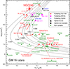 |
Fig. 1. Previously identified variable and nonvariable PG 1159 stars and variable [WCE] stars in the log Teff − log g diagram. The thin solid curves show the post-born again evolutionary tracks from Miller Bertolami & Althaus (2006) for different stellar masses. “Hybrid” refers to PG 1159 stars exhibiting H in their atmospheres, and “N.V.D.” means no variability data (which only applies to SDSS J152116). The location of the GW Vir star NGC 246 is shown as the large red star with error bars. This star is characterized by Teff = 150 000 ± 10 000 K and log g = 5.7 ± 0.10. |
The reported atmospheric parameters were derived using hydrostatic model atmospheres. This is justified because the star has a weak wind that only affects the formation of metal resonance lines in the ultraviolet wavelength region. Other spectral lines are not affected because they form in the hydrostatic layer of the atmosphere. The C IV 1548/1551 Å and O VI 1032/1038 Å resonance lines in NGC 246 display prominent P Cygni profiles, which were analysed with non-LTE wind models by Koesterke & Werner (1998) and Koesterke et al. (1998). A mass-loss rate of log Ṁ/(M⊙ yr−1) = −6.9 was measured. This value is significantly lower than the mass-loss rates of [WCE] central stars (the putative progenitors of PG1159 stars), for which mass-loss rates have been determined that are on average about an order of magnitude higher. As a consequence, the spectra of [WCE] stars are dominated by emission lines that form in the dense stellar wind. It is worth mentioning that weak stellar winds are not expected to affect the computed pulsation modes as their weight functions are small at the stellar surface during this part of the star’s evolution (see Figs. 5 and 8 of Kawaler et al. 1985 and Córsico & Althaus 2006, respectively).
In the first literature notes from Landolt (1983) and Grauer et al. (1987), this star was listed as a nonvariable star. Only a decade later, the observations of Ciardullo & Bond (1996), carried out on three nights, showed its low-amplitude pulsations. The first two (consecutive) nights revealed significant peaks at 683 and 648 μHz in the Fourier spectrum, while the last observation, nine months later, showed a different peak at 540 μHz. A more extensive study conducted by González Pérez et al. (2003) (three short runs carried out in 2000–2001) showed a complex and highly variable short-scale photometric behavior. In the 2000 observing run, the first night (2.2 h long) showed a peak around 550 μHz, while three days later the second night (3 h) showed a lower amplitude peak in the same region and also a stronger peak at 685 μHz. Observations from over a year later (more than 4 h long) showed a peak at ∼450 μHz and additional possible peaks located around 400 and 500 μHz. The last run was carried out two months later and, because of its poorer quality, only showed low-amplitude peaks at the same region as in the previous run. Moreover, the authors claimed possible features in the Fourier spectra that may be related to interactions with a close companion (e.g., alleged harmonics of the 450 μHz peak). All these observations, carried out over more than two decades, only proved that in order to reveal the details of the complex nature of the pulsations of the central star in NGC 246, extensive monitoring on a longer time base was very necessary. With a lack of a dedicated Whole Earth Telescope (WET) campaign (Nather et al. 1990), as already suggested by González Pérez et al. (2003), the TESS observations finally give us the exciting opportunity to study the complex behavior of the GW Vir star in NGC 246 in detail. A preliminary analysis of this star was presented by Aller et al. (2020).
The present work is the sixth in the series of papers dedicated to studying pulsating H-deficient WDs and pre-WDs observed with TESS. The first paper focused on the analysis of six already known GW Vir stars (Córsico et al. 2021), and the second paper on the discovery of two new stars of this type (Uzundag et al. 2021). In the third part Córsico et al. (2022b) analyzed the DBV star3 GD 358, while in the fourth (Uzundag et al. 2022) the discovery of two additional GW Vir stars was reported. In the fifth paper (Córsico et al. 2022a) the authors presented the discovery of two new DBV pulsators and the analysis of three already-known pulsating WD stars of this type.
This paper is organized as follows. In Sect. 2 we provide details of the observations and reduction of the photometric TESS data, and also of the frequency analysis. In Sect. 3 we start by giving a brief summary of the evolutionary models and numerical tools employed for our theoretical analyses. Next we focus on the asteroseismic modeling of NGC 246, including the search for a possible mean period spacing within the period spectra (Sect. 3.1), the derivation of the stellar mass using the inferred period spacing (Sect. 3.2), and the search for a period-to-period fit with the aim of finding an asteroseismic model that best represents the pulsations of the target star (Sect. 3.3). Finally, in Sect. 4 we summarize our main findings.
2. Observations and data reduction
NGC 246 was observed by TESS in Sector 3 between September 20 and October 18, 2018, and in Sector 30 between September 22 and October 21, 2020. In Sector 3 this star was observed during 20.27 days with the short-cadence (SC) mode, 120 s, with a 1.19-day gap between the orbits, which is shorter than the 27-day nominal duration of one-sector observations; in Sector 30 it was observed for 25.92 days with a 1.07-day gap in both SC and ultra-short-cadence mode (USC), 20 s. There is a 709.67-day data gap between the two sectors.
We first investigated the target-pixel files (TPFs) from TESS to assess the potential contamination from the nearby objects within the TESS aperture by using different aperture shapes, sizes, and systematics corrections. We downloaded TPFs for Sectors 3 and 30 in LIGHTKURVE (Lightkurve Collaboration 2018) for further processing. Then we created custom apertures, and used them to extract raw light curves from the TPFs. TPFs are already processed by the Science Processing Operations Center (SPOC) pipeline (Jenkins et al. 2016) that removes backgrounds, but it is still possible to remove common trends in TPF pixels. We found that Pixel-Level Decorrelation (PLD) (Deming et al. 2015) within LIGHTKURVE gave the best results compared to the Pre-search Data Conditioning Simple Aperture Photometry (PDCSAP) flux. PLD is a special case of a regression corrector that uses linear regression to remove systematic noise from light curves based on a design matrix created using only background pixels surrounding the target aperture. A noise model created using this information from nearby pixels is then subtracted from the uncorrected light curve.
In Fig. 2 we show the pipeline apertures used to extract photometry in Sectors 3 and 30, overlaid on the DSS2 Red image. It is evident that nebular contamination is small but inevitable, and it varies between the two sectors because of the different sizes of the apertures. The on-sky orientation of the field is almost the same; there is only a small shift (∼1 pix), and therefore the use of an aperture of the same shape (but slightly shifted) would be justified and perhaps more appropriate in this case.
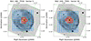 |
Fig. 2. TESS Sectors 3 and 30 pipeline aperture overlaid on DSS2 Red sky image. The target is marked with yellow circles. The blue squares show the TPF overlay and the red squares show the TPF aperture overlay for each sector. The figure was produced using mkpy3 by Kenneth Mighell (https://github.com/KenMighell/mkpy3). |
Figure 3 shows the target (Tmag = 12.31) with other stars from the TESS input catalog (Stassun et al. 2019). There are two main sources of contamination: the Tmag = 13.70 star close to the target position, which is the wide binary member of the NGC 246 triple system (HIP 3678 B), and the Tmag = 11.14 star, TYC 5272-1854-1, to the right. The TESS header contains two parameters for crowding correction: CROWDSAP, the crowding metric, defined as the ratio of the target flux to the total flux in the optimal aperture, and FLFRCSAP, the flux fraction, which reflects what fraction of the Pixel Response Function of the target is outside the optimal aperture (missing flux). In the case of NGC 246, the CROWDSAP value is 0.72 for Sector 3 and 0.64 for Sector 30, while FLFRCSAP is 0.72 and 0.78, respectively. It means that using solely the CROWDSAP, only 72 and 64% of the total flux originally measured in the aperture originates from the target in Sectors 3 and 30, respectively. The possible influence on the variability of NGC 246 by the 13.70 mag star is hard to assess with only TESS data at hand; therefore, we checked whether the 11.14 mag star shows any variability in the TESS data. We varied the aperture sizes and shapes for that target, and concluded that there was no variability from that star that could influence our analysis of NGC 246. With the ground-based data from González Pérez et al. (2006) reduced anew, using only a short run where it was possible to resolve the stars, we were not able to verify the lack of variability in the 13.70 mag star on timescales relevant to our analysis. Since HIP 3678 B is an early-to-mid K dwarf star (Adam & Mugrauer 2014), it is not expected to exhibit variability that we could confuse with pulsations of the white dwarf primary. Our new analysis of this dataset only confirms the findings reported by the authors that the Fourier spectrum was variable on a nightly basis.
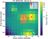 |
Fig. 3. TESS Target Pixel File (TPF) with the position of NGC 246 given by a white cross (×). The other sources in the field from Gaia DR2 are shown as red circles scaled according to magnitude. The aperture mask used by the PDC pipeline is shown with red squares. |
For the analysis presented in the remainder of the paper, we use the extracted times in Barycentric corrected Julian days (BJD-245700) and fluxes already corrected for contamination by the pipeline (PDCSAP FLUX) from the FITS files using LIGHTKURVE. The fluxes were normalized and transformed to amplitudes in units of parts per thousand (ppt). To remove the outliers that appear above five times the median of intensities, the data were finally sigma-clipped based on 5σ.
2.1. Frequency analysis
In order to analyze the periodicities in the data and determine the frequency of each pulsation mode, along with their amplitude and phase, Fourier transforms (FTs) of the light curves were computed. We chose a 0.1% false alarm probability (FAP) detection threshold, which means that if the amplitude exceeds this threshold, there is a 0.1 percent chance that it is merely the result of noise fluctuations. Following the procedure outlined in Kepler (1993), we determined the 0.1% FAP threshold. We performed a nonlinear least-squares (NLLS) fit in the form of Aisin(ωit + ϕi), with ω = 2π/P, where P is the period. We identified the frequency (period), phase, and amplitude values for each periodicity in this way. We pre-whitened the light curves using the NLLS fit parameters until, excepting unresolved peaks, there was no longer any significant signal in the FT of both datasets above the significance level of 0.1% FAP. All pre-whitened frequencies for NGC 246 are given in Table 1, where we present frequencies (periods) and amplitudes, along with their corresponding errors and the signal-to-noise ratio (S/N). The average noise level of Sector 3 corresponds to 0.06 ppt and the significance level of 0.1% FAP, to 0.29 ppt. We extracted 15 frequencies above 0.29 ppt from the light curve, as shown in the top panel of Fig. 4. All the pulsational frequencies are located between 548 μHz (1822 s) and 684 μHz (1459 s). For Sector 30, the average noise level corresponds to 0.055 ppt. In total, we detected 12 pulsational frequencies above the detection threshold of 0.26 ppt. This case is shown in the bottom panel of Fig. 4. In Table 1 we report the final best-fit values for the frequencies (periods) and amplitudes of the individual sinusoids in our model.
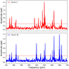 |
Fig. 4. Fourier transform of Sector 3 (upper panel) and Sector 30 (lower panel) of NGC 246. The horizontal red line indicates the 0.1% FAP level. |
Frequency solution from the light curves of Sectors 3 and 30 of NGC 246 including frequencies, periods, amplitudes (and their uncertainties), and S/N.
2.2. Possible rotational multiplets
As we show here, the identification of the value of ℓ is a critical component of an asteroseismic analysis. One property of nonradial pulsations in compact stars, the effects of rotation, often provides critical data used to identify the value of ℓ (and m). For a nonrotating star, the pulsation frequencies for modes with the same value of k are the same for all values of ℓ and m. Rotation, however, can lift that degeneracy, splitting modes with different sets of (ℓ, m) by amounts proportional to the rotation frequency Ω. As long as the rotation frequency is significantly lower than the pulsation frequency (i.e. to first order in Ω/σk), we have
 (1)
(1)
where σk is the oscillation (angular) frequency in the nonrotating case, and Ck, ℓ is a function (integrated through the star) of the stellar structure and the eigenfunctions for the mode (for details, see, e.g., Aerts et al. 2010).
Thus, rotation can produce a triplet of ℓ = 1 modes, with a central peak (m = 0) flanked by peaks separated on either side by Ω(1 − Ck, ℓ). Higher ℓ modes can be split into multiplets with 2ℓ+1 components, split equally by the same factor (though the value of Ck, ℓ depends on ℓ).
For g modes in compact stars, where the horizontal displacement is much larger than the radial displacement, the value of Ck, ℓ is closely approximated by (Winget et al. 1991)
 (2)
(2)
which means for ℓ = 1 modes that the (angular) frequency spacing between peaks in the FT is Ω/2, while for ℓ = 2 modes we would (ideally) see a quintuplet of modes, split by Ω × 5/6. The rotational splitting of all modes (all values of k) of a given ℓ should be identical unless there is latitudinal differential rotation. If both ℓ = 1 and ℓ = 2 modes are excited in the star, the values of their rotational splitting should be related by exactly  .
.
If the rotational period is not longer than the duration of the observation, this 2ℓ + 1 configuration can be resolved using high-precision photometry. Rotational multiplets have been detected for all types of pulsating WDs, including GW Vir, DBV, DAV4, and ELMV5 stars; the derived rotation periods range from 1 hour to a few days (Hermes et al. 2017; Córsico et al. 2019, 2022a; Lopez et al. 2021; Uzundag et al. 2022; Calcaferro et al. 2023).
For a rotation period of 1 or 2 days, the ℓ = 1 splitting corresponds to 5.79 or 2.89 μHz, respectively. The ℓ = 2 splitting is larger (see Eq. (2)) by a factor of 5/3. In most of the cases cited above, the frequency splitting between peaks in a given (k, ℓ) multiplet is significantly smaller than the spacing between modes of different k. Instead, for pulsating PN central stars, which have periods that are significantly longer, the separation in frequency between modes of different k is smaller. For the long periods (like those detected in NGC 246), the period spacing between consecutive m = 0 modes results in a small frequency spacing that can be confused with the rotational splitting, so care must be exercised to separate the two effects (similar issues arose in the study of the central star of NGC 1501 by Bond et al. 1996).
With this theoretical background, we attempted a search for frequency splittings within the detected frequencies. First, we searched for pairs of peaks with a similar frequency separation. Frequencies f10,S03 and f11,S03 differ by 641.829 − 639.872 = 1.957 μHz, while frequencies f14,S03 and f15,S03 by 664.997 − 661.711 = 3.286 μHz. The relation between these separations is almost exactly 0.6, and therefore we might suspect that f10,S03 and f11,S03 could be ℓ = 1 modes, whereas f14,S03 and f15,S03 could be ℓ = 2 modes, both cases with missing components. Another pair of ℓ = 1 modes could be f3,S03 and f4,S03: 565.800 − 563.500 = 2.300 μHz. On the other hand, the frequency splitting might be larger, as we found four sequences split by approximately 5 μHz (it could even be a sequence of five modes, f6 − f10):
f1,S03 and f2,S03: 553.725 − 548.646 = 5.079 μHz;
f6,S03 and f7,S03: 624.294 − 619.230 = 5.064 μHz;
f9,S03 and f10,S03: 639.872 − 634.850 = 5.022 μHz; and
f13, S30 and f14, S30: 661.506 − 656.412 = 5.094 μHz.
If these modes were ℓ = 1 we could expect the ℓ = 2 modes split by about 8.4 μHz, otherwise we could expect the ℓ = 1 modes split by about 3 μHz. We did not find any clear sequences with these values other than the ones already mentioned, and therefore we explored the possibility of overlapping mode sequences with missing components. For example, if we consider the difference between f7,S03 and f11,S03 of 641.829 − 624.294 = 17.535 μHz, it could be a triplet of ℓ = 2 modes with a missing component in between split by 8.767 μHz (and missing side components), overlapping in the same region as previously mentioned ℓ = 1 modes split by about 5 μHz. A multitude of options prevent us from a definitive determination of the rotation period in NGC 246 and mode identification based on the observed frequency splitting.
3. Asteroseismic analysis
The asteroseismic analysis performed in this work is based on a set of stellar models that take the complete evolution of the PG 1159 progenitor stars into account (Althaus et al. 2005; Miller Bertolami & Althaus 2006, 2007a,b). Post-AGB evolutionary sequences, computed with the LPCODE evolutionary code (Althaus et al. 2005), were followed through the very late thermal pulse (VLTP) episode and the resulting born-again episode that leads to the H-deficient, He-, C-, and O-rich composition expected for PG 1159 stars. The resulting stellar remnants have masses of 0.515, 0.530, 0.542, 0.565, 0.589, 0.609, 0.664, 0.741, and 0.870 M⊙. In Fig. 1, the evolutionary tracks corresponding to the PG 1159 models employed in this work are shown in the log(Teff)−log(g) plane. Details about the input physics and evolutionary calculations carried out to obtain the PG 1159 evolutionary sequences employed in this work can be found in Althaus et al. (2005) and Miller Bertolami & Althaus (2006, 2007a,b). We computed ℓ = 1, 2 g-mode adiabatic pulsation periods in the range 80–6000 s with the adiabatic version of the pulsation code LP-PUL (Córsico & Althaus 2006). We analyzed roughly 4000 PG 1159 models covering a wide range of effective temperatures (4.8 ≲ log Teff ≲ 5.4), luminosities (0 ≲ log(L⋆/L⊙)≲4.2), and stellar masses (0.515 ≤ M⋆/M⊙ ≤ 0.870).
The nonradial g modes that cause brightness variations in WDs and pre-WDs can be excited in a sequence of consecutive radial orders, k, for a given value of the harmonic degree, ℓ. In the asymptotic limit of high radial order, the periods of g modes with consecutive radial orders are approximately evenly separated; the period spacing is dependent on ℓ, according to the expression (Tassoul et al. 1990)
 (3)
(3)
where Π0 is a constant value given by
![Mathematical equation: $$ \begin{aligned} \Pi _0=\frac{2\pi ^2}{\left[\int ^{r_2}_{r_1}{\frac{N}{r}\mathrm{d}r}\right]} \end{aligned} $$](/articles/aa/full_html/2024/06/aa49103-23/aa49103-23-eq7.gif) (4)
(4)
and N is the Brunt-Väisälä frequency. In the case of chemically homogeneous stellar models, this formula for the asymptotic period spacing ( ) represents a precise description of the separation of consecutive g-mode periods for large radial orders. A very relevant property of the g-mode period spacing of pulsating PG 1159 stars is that it primarily depends on the stellar mass, and only weakly on the luminosity and the He-rich envelope mass (Kawaler 1986, 1987, 1988, 1990; Kawaler & Bradley 1994; Córsico & Althaus 2006). This property, in principle, can be used to derive the mass of a star by measuring the period spacing. For chemically stratified stars, such as PG 1159 stars, the g-mode period spacings considerably depart from uniformity due to the mechanical resonance called “mode trapping” (Kawaler & Bradley 1994). Therefore, at first glance, it would seem that the observed period separation of a chemically stratified star could not be used to infer its stellar mass. Fortunately, the average value of the period spacings in chemically layered PG 1159 stars still preserves the property of being a function almost exclusively of the stellar mass (Tassoul et al. 1990). Thus, it is still possible to derive the stellar mass of chemically stratified stars from the comparison between the observed mean spacing of periods, ΔΠ, and the average of the period spacings,
  , calculated for sets of PG 1159-star models with different masses and effective temperatures.
Another approach to deriving the stellar mass, which can give information about the internal structure of the pulsating star at the same time, is to search for a pulsation model that best matches the individual pulsation periods of the star under study. The goodness of the match between the theoretical pulsation periods ( ) and the observed individual periods (
 ) is measured by means of a merit function defined as
![Mathematical equation: $$ \begin{aligned} \chi ^2(M_{\star }, T_{\rm eff})= \frac{1}{m} \sum _{i=1}^{m} \min \left[\left(\Pi _i^\mathrm{O}- \Pi _k^\mathrm{T}\right)^2\right], \end{aligned} $$](/articles/aa/full_html/2024/06/aa49103-23/aa49103-23-eq12.gif) (5)
(5)
where m is the number of observed periods. The PG 1159 model that shows the lowest value of χ2, if it exists, is adopted as the best-fit model. We assess the function χ2 = χ2(M⋆, Teff) for stellar masses of 0.515, 0.530, 0.542, 0.565, 0.589, 0.609, 0.664, 0.741, and 0.870 M⊙. For the effective temperature we employ a much finer grid (ΔTeff = 10 − 30 K), which is given by the time step adopted by our evolutionary calculations.
The mentioned methods used to estimate the stellar mass and the internal structure of NGC 246 are the same as we employed in our previous works at the La Plata Stellar Evolution and Pulsation Research Group6 (e.g., Córsico et al. 2007a,b, 2008, 2009, 2021; Kepler et al. 2014; Calcaferro et al. 2016; Uzundag et al. 2021), where further details can be found.
3.1. Period spacing
As a first step, we estimated a mean period separation underlying the observed periods (if it exists). Considering the set of periods from Table 1, we searched for a constant period spacing within the data of NGC 246 employing the Kolmogorov-Smirnov (KS; see Kawaler 1988), the inverse variance (IV; see O’Donoghue 1994), and the Fourier transform (FT; see Handler et al. 1997) significance tests. Given that, in principle, there are two different sets of periods coming from two sectors, we followed this procedure for each set of periods separately. We also considered a combination of the two sets, taking the average value for those cases where two periods are identified as the same mode. We show the resulting list of 17 periods in the first column of Table 2. Since we found similar solutions for the three cases, we only show the results for the case of the 17 periods from the combined sectors (Table 2) in Fig. 5, indicated with dotted black lines. The figure shows a clear signature of a potential mean period spacing around 12.9 s, while other possible values are around 10.6, 14.5, and 51 s. Next, we repeated this analysis but employing other sets of periods. In our trials we found that, for instance, when discarding the periods at around 1503, 1511, 1557, 1562, 1767, and 1774 s, the three statistical tests applied to the resulting set of 11 periods show more robust evidence of a mean period spacing at ∼12.9 s, as depicted with solid orange lines in Fig. 5, while the other possible values show much lower (or no) statistical significance, and hence we disregarded them. The addition or removal of some of these excluded periods gives approximately the same results, in some cases even improving the statistical significance of the tests. In this way, we adopted the value of ∼12.9 s as a guess value for the mean period spacing.
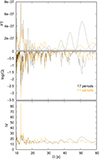 |
Fig. 5. Significance tests applied to the period spectrum of NGC 246 to search for a constant period spacing: FT (upper panel), K-S (middle panel), and IV (bottom panel). The dotted black lines represent the results for the set of 17 periods from Table 2, while the solid orange lines represent the case for a subset of 11 periods (see text for details). |
List of the 17 periods combined from Sectors 3 and 30 for NGC 246.
We cannot know in advance if this possible mean period spacing is associated with ℓ = 1 or 2 modes. We might assume it is a period spacing of ℓ = 2 modes for its short value, but then a period spacing of 22.3 ( , according to Eq. (3)) corresponding to ℓ = 1 modes would be expected, which is absent. However, there is no reason to discard this 12.9 s period spacing for a sequence of ℓ = 2 modes. In the following section we estimate the stellar mass of NGC 246 by considering the possibility that ΔΠ = 12.9 s is associated with ℓ = 1 or ℓ = 2 modes.
To derive a refined value of the period spacing first we carried out a linear least-squares fit, using the reduced set of 11 periods. We obtained ΔΠ = 12.934 ± 0.054 s. The average value of the residuals (δΠ) resulting from the difference between the observed periods and those calculated from the mean period spacing is 1.093 s. We repeated the linear least-squares fit, but this time, including three of the previously discarded periods (1511, 1562, and 1767 s; i.e., we used the 14 periods flagged with an asterisk in Table 2) that are compatible with the previous linear fit, and we obtained ΔΠ = 12.902 ± 0.045 s. This value of the period spacing is slightly smaller than the one derived previously, and the uncertainty is slightly smaller. Additionally, the average of the residuals is smaller (0.986 s) so the fitted periods match the observed periods better than before, and this is why we adopt ΔΠ = 12.902 ± 0.045 s as the definitive value for the mean period spacing of NGC 246. In Table 2 we indicate the theoretical periods from the fitted mean period spacing (second column) and the corresponding residuals (third column). In the last column, we indicate the possible identification of the fitted periods with ℓ = 1 modes, according to the period spacing previously inferred, although they may all be associated with ℓ = 2, as already mentioned. In addition, we show the corresponding linear fit in the upper panel of Fig. 6, while the residuals for this case are displayed in the lower panel. It is worth noting the presence of some minima in the distribution of the residuals, which can be attributed to the effects of mode trapping caused by the existence of internal chemical transition regions (Kawaler & Bradley 1994).
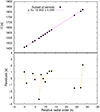 |
Fig. 6. Results of the linear least-squares fit to refine the period spacing value. Upper panel: linear least-squares fit applied to a subset of 14 periods of NGC 246 (see text for details). The resulting period spacing is ΔΠ = 12.902 ± 0.045 s. Lower panel: residuals of the period distribution relative to the dipole mean period spacing. A thin orange line connects modes with consecutive radial order. |
3.2. Mass determination from the comparison between the observed mean period spacing and the average of the computed period spacings
We then determined the mass of NGC 246 by comparing the average of the computed period spacings,  , for our grid of models with the observed period spacing, ΔΠ, as determined in Sect. 3.1. The average of the computed period spacings is calculated as
  , where the “forward” period spacing is defined as ΔΠk = Πk + 1 − Πk (k being the radial order) and n is the number of theoretical periods within the range of the periods observed in the target star. For this star, Πk ∈ [1459, 1823 s].
In Fig. 7 we show the run of the average of the computed period spacings for NGC 246 for the case in which the period spacing is assumed to be associated with ℓ = 1 modes, indicated with thin curves, and ℓ = 2 modes, represented with thick curves, in terms of Teff for our PG 1159 evolutionary sequences. The location of NGC 246 in this  plane is represented by a black circle with error bars, where we used the period spacing (and its uncertainty) determined in Sect. 3.1, and the star’s effective temperature (with a 10% for its uncertainty, which is slightly higher than that given by the latest spectroscopic results). Clearly, for each set of curves with ℓ = 1 and 2, the lower the values of
  , the higher the stellar mass. When we consider the measured period spacing ΔΠ = 12.902 ± 0.045 s to be associated with ℓ = 1 modes, it is clear that the stellar mass is slightly higher than 0.87 M⊙. Instead, if we consider that the period spacing corresponds to ℓ = 2 modes, a linear interpolation between ΔΠ and
  7 yields a stellar mass of
  .
.
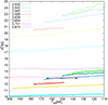 |
Fig. 7. Average of the computed period spacings, |

PG 1159 stars with these two candidate seismic masses would have significantly different absolute magnitudes. We can compute the distances that the models would have to be at to match the apparent magnitude observed for NGC 246 by following a procedure similar to previous works in this series (see also Bell et al. 2019; Uzundag et al. 2023). The apparent visual magnitude of NGC 246, mV, is 11.8 mag (Zacharias et al. 2012), while the interstellar absorption AV(d) = RVE(B − V) (with RV = 3.1) for this star is 0.062 mag, according to Frew et al. (2016) and Ali et al. (2023). Using the bolometric correction extracted from the grids of He-atmosphere WDs of the Montreal Group8 (Bergeron et al. 1995; Holberg & Bergeron 2006; Bédard et al. 2020), the visual absolute magnitude is calculated as MV = MB − BC, where MB = MB⊙ − 2.5 × log(L⋆/L⊙) and MB⊙ = 4.74 (Cox 2000). In this way the distance, d, can be inferred from log(d) = [mV − MV + 5 − AV(d)]/5. A plot of distances computed for our PG 1159 evolutionary models of different masses is shown in Fig. 8. The error bars indicate the distance estimate,  pc (Bailer-Jones et al. 2021), and the spectroscopic effective temperature. Using other reported values of the interstellar absorption for this star, AV = 0.14 mag (González-Santamaría et al. 2021) and AV = 0.0806 mag resulting from the value of E(B − V) obtained from the 3D reddening map (Lallement et al. 2014, 2018; Capitanio et al. 2017)9 according to the galactic coordinates of this star
  does not significantly change the resulting distance estimations (the difference being within a few tens of parsec). While neither candidate mass suggested by the mean period spacing falls in the one-sigma error box, the lower-mass models are more compatible with the astrometric distance, leading us to favor the interpretation that we are observing an overtone sequence of ℓ = 2 modes and the corresponding
  mass.
mass.
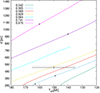 |
Fig. 8. Inferred distance for our PG 1159 evolutionary models to match the observed apparent magnitude of NGC 246, in terms of effective temperature. The symbol with error bars marks the effective temperature reported from spectroscopy and the distance constraint from Gaia astrometry. The four individual models that achieve the best fits to the individual pulsation periods are marked with asterisks (see discussion in text). |
In closing this section, it is worth mentioning that these two candidate seismic masses would have different surface gravity as well: the one with ∼0.87 M⊙ at ∼150 000 is characterized by log g ∼ 5.52, while the one with 0.568 M⊙ at ∼150 000 by ∼6.29. Considering that the value given by spectroscopy for NGC 246 is 5.7, the former has a more similar value.
3.3. Constraints from the individual observed periods: Searching for the best-fit model
We now turn to fitting the pulsation modes to stellar models to try to derive the stellar mass and compare the results with those obtained with the mean period spacing. This procedure, as already explained, may allow us to determine the mode identification of individual modes. To carry this procedure out, we took different sets of periods into account: each set of periods from Sectors 3 and 30 from Table 1, and the combination of the two, as indicated in Table 2. In this last case we also considered two particular subsets of the combination: one subset with 11 periods (see Sect. 2.2), and another with the 14 periods (flagged with asterisks in Table 2) that fit the mean period spacing determined in Sect. 3.1. For all cases we first considered that all the periods are associated with ℓ = 1 g modes and employed them to assess the quality function given by Eq. (5). Next, we repeated the procedure, but assumed that periods result from a mixture of ℓ = 1 and ℓ = 2 g modes. Generally, if a single maximum exists, we can adopt the corresponding model as the asteroseismic solution. Unfortunately, in the cases we studied here there are multiple possible solutions, and thus we needed to apply an external constraint in order to adopt a single asteroseismic model. In this case the constraint is the effective temperature and its uncertainty, where again we took a more flexible value than the one given by spectroscopy.
We started by considering the list of 15 periods from Sector 3 (Table 1); we show the results for the ℓ = 1 case in the upper left panel of Fig. 9. In the figure we plot the inverse of the quality function, 1/χ2, such that the greater the value of 1/χ2, the better the fit between theoretical and observed periods. It is clear that there is more than one possible asteroseismic solution. In particular, the absolute maximum (the best solution) in this case corresponds to a model with Teff ∼ 196 000 K, which is much higher than the values of Teff allowed by the spectroscopic determinations for NGC 246, and can be discarded. The second-best global fit lies within the constraints given by the allowed range of effective temperatures at ∼140 000 K, for M⋆ = 0.741 M⊙ and 1/χ2 = 0.117. When we consider the list of 12 periods from Sector 30 (Table 1), and repeat the above procedure, we obtain the results shown in the upper right panel of Fig. 9. Once again, there are multiple possible solutions, but the best global fit lies within the range of allowed Teff at ∼160 000 K, for 0.87 M⊙ and 1/χ2 = 0.096. Next we considered the set of 17 periods combining Sectors 3 and 30, which are listed in Table 2. The results are shown in the middle panel of Fig. 9. The best global fit lies at a very high Teff, and within the ranges of allowed Teff, there is a possible solution characterized by ∼140 000 K, for 0.741 M⊙ and 1/χ2 = 0.097. The lower left panel of Fig. 9 depicts the results when considering the subset of 11 periods. In this case, the best global fit lies at high values of Teff. However, in the allowed ranges of Teff, there is a possible solution characterized by ∼140 000 K, for 0.741 M⊙, and 1/χ2 = 0.116. The results for the subset of 14 periods are shown in the lower right panel of Fig. 9. Similarly to the previous case, although the best global fits lie at very high values of Teff, there are some possible solutions, with comparable quality, given by ∼160 000 K for 0.870 M⊙ and 1/χ2 = 0.092, and ∼140 000 K for 0.741 M⊙ and 1/χ2 = 0.083. It is clear from the figure that the S03 results (15 periods; first panel) are similar to the S03+30 results (11 periods; lower left panel).
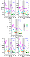 |
Fig. 9. Inverse of the quality function, 1/χ2, vs. Teff of the period-to-period fits in the ℓ = 1 case, for the five sets of periods considered for NGC 246: Sector 3 (upper left panel), Sector 30 (upper right panel), the 17 periods from the combination of both sectors (middle panel), and the two subsets of the combination of both sectors with 11 periods (lower left panel) and 14 periods (lower right panel). The vertical gray strip indicates the spectroscopic values of Teff and the corresponding uncertainty for this star. |
We show the results of the ℓ = 1, 2 case in Fig. 10. The quality of the solutions is in general improved, as evidenced by the greater values of 1/χ2. The results for the set of periods from Sector 3 are shown in the upper left panel. The best global fits are located at higher and lower values of Teff than those given by spectroscopy. However, there are possible solutions within the allowed ranges of Teff at ∼160 000 K, for 0.870 M⊙ and 1/χ2 = 0.356; at ∼140 000 K, for 0.741 M⊙ and 1/χ2 = 0.313; and also at ∼163 000 K, for 0.565 M⊙ and 1/χ2 = 0.301. For Sector 30, as shown in the upper right panel of Fig. 10, the best solution has a very low Teff, and the solutions that lie within the range of allowed Teff are characterized by ∼160 000 K, 0.741 M⊙, and 1/χ2 = 0.412, and ∼163 000 K, 0.565 M⊙, and 1/χ2 = 0.361. For the combined set of periods from both sectors, as the middle panel of Fig. 10 depicts, the best-fit models have very high values of Teff. Still, there are three possible solutions within the range of allowed Teff that are worth mentioning at ∼163 000 K, for 0.565 M⊙ and 1/χ2 = 0.335; at ∼160 000 K, for 0.870 M⊙ and 1/χ2 = 0.303; and also at ∼140 000 K, for 0.741 M⊙ and 1/χ2 = 0.289. The case of the subset with 11 periods, represented in the lower left panel of Fig. 10, shows the best global fit for a model characterized by ∼150 000 K, 0.565 M⊙, and 1/χ2 = 0.654. Other possible solutions within the range of allowed Teff are characterized by ∼140 000 K, 0.741 M⊙, and 1/χ2 = 0.589; ∼157 000 K, 0.565 M⊙, and 1/χ2 = 0.573; and ∼163 000 K, 0.565 M⊙, and 1/χ2 = 0.574. Finally, the lower right panel of Fig. 10 depicts the results for the subset with 14 periods. In this case the best global fit is represented by a model with ∼163 000 K, 0.565 M⊙, and 1/χ2 = 0.681. It is worth mentioning that this solution has the best quality (the highest value of 1/χ2) among all the cases considered in this work. Other possible solutions that also lie within the range of allowed Teff are characterized by models with ∼157 000 K, 0.565 M⊙, and 1/χ2 = 0.607, and ∼150 000 K, 0.565 M⊙, and 1/χ2 = 0.537.
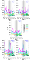 |
Fig. 10. Same as Fig. 9, but for the ℓ = 1, 2 case. The 1/χ2 values are much higher than for the ℓ = 1 case (Fig. 9), indicating that these models fit the data better. The middle panel demonstrates that there is not a particularly preferred model fit in the case of all 17 periods from the combined sectors. In the two bottom panels, the 0.565 M⊙ sequence has several models that fit the data well within the observed temperature bounds. In the 11-period case there is also a 0.74 M⊙ model that fits. |
When we compare the results from all cases it is clear that the global behavior of the quality function changes, although some solutions are repeated in more than one case. Within the allowed ranges of Teff four solutions stand out. When using only ℓ = 1 modes, and also when using a mixture of ℓ = 1, 2 modes, there are possible seismic solutions characterized by 0.741 M⊙ and ∼140 000 K, and 0.870 M⊙ and ∼160 000 K. On the other hand, if we consider ℓ = 1, 2 modes, there are also possible seismic solutions with 0.565 M⊙ and ∼163 000 K, and 0.565 M⊙ and ∼150 000 K.
Although it is not possible to adopt one solution, it is of interest to study whether there is agreement between the data residuals and the model residuals of an asteroseismic solution, instead of only comparing the individual periods. We did this with our possible asteroseismic solutions, but we only show the case of the model with 0.565 M⊙ and ∼163 000 K in Fig. 11, given that it has the highest 1/χ2 value for all the cases considered in this work. In the figure we plot the residuals of the period distribution relative to the observed period spacing (black points, as in the bottom panel of Fig. 6) in terms of the relative radial order, along with the corresponding residuals for the mentioned theoretical model. As can be seen, there is a moderate agreement between the two.
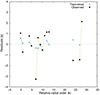 |
Fig. 11. Distribution of the residuals relative to the mean period spacing for the case of the observed periods (black points, see bottom panel of Fig. 6), along with the case for the theoretical periods (sky blue crosses) of the model fit with 0.565 M⊙ and ∼163 000 K, represented in terms of the relative radial order. As in Fig. 6, the thin lines connect modes with consecutive radial order. |
Given these four best-fitting models, we calculate their asteroseismic distances and compare them with the distance resulting from the Gaia measurements. The masses, temperatures, luminosities, and inferred distances for these models are listed in Table 3, and these models are marked with asterisks in Fig. 8. It is clear that none of these four candidate models falls within the uncertainties of the precise distance constraint from Gaia.
Properties and inferred distances for four best-fitting seismic models.
Finally, a calculation of the stellar mass when fixing the distance of NGC 246 to the value given by Gaia for different values of AV and some effective temperatures in the range of interest results in model sequences characterized by a stellar mass around 0.6 M⊙. For the resulting luminosities to be compatible with stellar masses ≳0.7 M⊙, AV should be ≳1.3 mag, which would be too large and inconsistent with the high value of the galactic latitude of NGC 246 below the Galactic plane ( ).
).
4. Summary and discussion
In this paper we presented a detailed asteroseismic study of NGC 246, a pulsating PG 1159 star, based on the high-precision photometry data from TESS observations. NGC 246 (Teff ∼ 150 000 K and log g ∼ 5.7) was observed by TESS in Sector 3 at the short 120 s cadence, and in Sector 30, at the short 120 s and ultra-short 20 s cadence. Our frequency analysis revealed a total of 17 periodicities. These oscillation periods (1460–1823 s) are associated with nonradial g modes. Given this frequency spectrum, we investigated the presence of rotation multiplets. However, we did not find any distinct indications of rotational splitting for either dipole or quadrupole modes.
Employing the inferred pulsation periods, we carried out an asteroseismic analysis on NGC 246 by means of our fully evolutionary models of PG 1159 stars. We first found a constant period spacing underlying the observed periods that was used to make inferences on the stellar mass via the comparison between the observed mean period spacing and the average of the computed period spacings. Our results indicate that if the observed mean period spacing is associated with ℓ = 1 g modes, then M⋆ ≳ 0.87 M⊙. Instead, if it is associated with ℓ = 2 g modes, then M⋆ ≳ 0.568 M⊙. Next, we searched for the best-fit model between the theoretical and the observed periods. For this procedure we first assumed that all the periods were associated with ℓ = 1 g modes only, and subsequently with a mixture of ℓ = 1, 2 g modes. Although we did not find a clear and unambiguous solution for NGC 246, there are some possible solutions that lie within the values of effective temperature (for which we took an error of ±10%). When considering that all modes are ℓ = 1 only, our results suggest a high stellar mass (≳0.74 M⊙), but when we allow the modes to take a mixture of ℓ = 1 and 2, both high (≳0.74 M⊙) and intermediate (∼0.57 M⊙) stellar masses fit the data well. It is worth mentioning that the ℓ = 1 fits have lower 1/χ2 values than the ℓ = 1, 2 fits. A comparison between the corresponding asteroseismic distances for these models to the Gaia astrometric distance ( pc, Bailer-Jones et al. 2021) indicates that only one solution is in agreement, which corresponds to a model with M⋆ = 0.565 M⊙, lying at approximately the same Teff of the star.
NGC 246 has recently been analyzed by Löbling (2018, 2020) who, employing new spectroscopic observations and state-of-the-art non-LTE models, found Teff = 150 000 ± 10 000 K and log g = 5.7 ± 0.1. This results in  M⊙, and then in a stellar radius of R⋆ = 0.20 R⊙. Interestingly, in the spectral analysis carried out by Rauch & Werner (1997), the authors noted unusually broad spectral line cores, which was interpreted as a signature of stellar rotation with velocity v sin i ≈ 70 km s−1, where i is the unknown inclination angle of the rotation axis. This value was later confirmed by using high-resolution spectra by Rauch et al. (2004). More recently, Löbling (2018) measured v sin i = 75 ± 15 km s−1. Considering the latter along with the stellar radius derived from spectroscopy, this would imply a rotational period of P × sin i = 0.68 ± 0.14 d. If this were the rotational period that characterizes NGC 246, a rotational splitting of 8.51 μHz would be expected in the frequency spectrum in ℓ = 1 modes. However, neither of the amplitude spectra (of Sector 3 or 30) exhibits a clear pattern that would confirm this expectation. Still, it must be noted that the rotational velocity could be overestimated; for example, microturbulent motions in the atmosphere could contribute to the line-core broadening. Additionally, Löbling (2020) determined a spectroscopic distance of 970 ± 200 pc for NGC 246. This is a factor of 1.7 larger than the Gaia distance. In order to bring the spectroscopic distance in agreement with the parallax distance, an increase in the surface gravity by a factor of three (i.e., an increase of 0.5 dex in log g) would be necessary. As demonstrated by Löbling (2020), such a high value for the gravity strongly contradicts the model fits to the He II line profiles. The reason for this problem remains unknown. Interestingly, our possible asteroseismic solution with 0.565 M⊙ and ∼150 000 K, has a value of log g (=6.29), which is in line with the value needed to fit the parallax distance.
In addition to the distance resulting from the Gaia parallax value, two independent estimations for the distance to NGC 246 were performed in the past. First, by fitting the resolved companion to the zero age main sequence, Bond & Ciardullo (1999) found a distance of  pc, which is in agreement with the parallax distance. Second, from the observed angular expansion rate of the PN (Liller et al. 1966) and a measurement of the expansion velocity, Terzian (1997) found a distance of 570 pc. However, the errors in the expansion rate and velocity must be regarded as too high to favor either the parallax or the spectroscopic distance. Modern precise determinations of expansion rates of three PNe in a distance of about 2 kpc using HST imaging over four years were successfully performed by Palen et al. (2002). In principle, such measurements are also feasible for NGC 246, and could be compared to the precise astrometry measurements.
All in all, our results show two possible outcomes in the derivation of the stellar mass. The use of the pulsation periods via the comparison between the observed period spacing and the average of the computed period spacings points to a very high-stellar-mass asteroseismic model if the derived mean period spacing is associated with ℓ = 1 g modes, and an intermediate-stellar-mass model if, instead, it is associated with ℓ = 2 g modes. Although we were not able to adopt an asteroseismic model from the period-to-period fits, the results obtained from the different sets of periods considered in this procedure would indicate high-stellar-mass models for the ℓ = 1 case, and both high- and intermediate-stellar-mass models for the ℓ = 1, 2 case. Astrometry, by means of the precise measurements from Gaia, seems to point toward intermediate stellar masses, making one of our possible asteroseismic solutions particularly promising. At the same time, abiding by the precise distance from Gaia, our asteroseismological results may indicate that the set of modes of this star should be a mixture of ℓ = 1, 2. Regarding the stellar rotation, the conclusions derived from the spectroscopic analysis are not consistent with the precise astrometric distance, an aspect that cannot be ignored. Concurrently, asteroseismology has not yet provided a conclusive value for the rotation period.
Our lack of conclusive results shows the enigmatic nature of NGC 246. At this point, isolating the specific reason(s) behind the disparities among spectroscopic, seismological, and astrometric (Gaia) masses remains elusive, and further work is clearly required. Hopefully, future follow-up observations from space, such as the PLAnetary Transits and Oscillations mission (PLATO, Piotto 2018), or a ground-based program, such as BlackGEM (Bloemen et al. 2015), might help shed some light on this open problem. Additionally, improved atmospheric parameters from high-resolution spectroscopic data are necessary to put better constraints on the modeling and, possibly, to help mitigate the discrepancies found in this work.
Even though white dwarf stars of spectral type DO do not pulsate, the term “DOVs” has historically been used as a variable star designation for GW Vir pulsators without a nebula.
Although NGC 246 is the name of the planetary nebula, for simplicity throughout this work we use this designation to refer to the central star.
DBVs are He-rich atmosphere pulsating WD stars with effective temperatures and surface gravities in the ranges 22 400 ≲ Teff ≲ 32 000 K and 7.5 ≲ log g ≲ 8.3, respectively (Córsico et al. 2019).
DAVs are H-rich atmosphere pulsating WD stars with effective temperatures and surface gravities in the ranges 10 400 ≲ Teff ≲ 12 400 K and 7.5 ≲ log g ≲ 9.1, respectively (Córsico et al. 2019).
ELMVs are H-rich atmosphere pulsating extremely low-mass (ELM) WD stars with effective temperatures and surface gravities in the ranges 7 800 ≲ Teff ≲ 10 000 K and 6.0 ≲ log g ≲ 6.8, respectively (Córsico et al. 2019).
When there were no points to perform the linear interpolation, we extrapolated the theoretical values of  .
.
Acknowledgments
We want to thank our anonymous referee for the comments and suggestions that greatly improved the original version of the paper. Part of this work was supported by AGENCIA through the Programa de Modernización Tecnológica BID 1728/OC-AR, and by the PIP 112-200801-00940 grant from CONICET. This research was supported in part by the National Science Foundation under Grant No. NSF PHY-1748958, which enabled the KITP Program on White Dwarfs as Probes of the Evolution of Planets, Stars, the Milky Way and the Expanding Universe in 2022, at which some of this work was performed. M. U. gratefully acknowledges funding from the Research Foundation Flanders (FWO) by means of a junior postdoctoral fellowship (grant agreement No. 1247624N). PS and GH thank the Polish National Center for Science (NCN) for supporting the study through grants 2015/18/A/ST9/00578 and 2021/43/B/ST9/02972. This paper includes data collected with the TESS mission, obtained from the MAST data archive at the Space Telescope Science Institute (STScI). Funding for the TESS mission is provided by the NASA Explorer Program. This work has made use of data from the European Space Agency (ESA) mission Gaia (https://www.cosmos.esa.int/gaia), processed by the Gaia Data Processing and Analysis Consortium (DPAC, https://www.cosmos.esa.int/web/gaia/dpac/consortium). Funding for the DPAC has been provided by national institutions, in particular, the institutions participating in the Gaia Multilateral Agreement. This research has made use of NASA’s Astrophysics Data System Bibliographic Services, and the SIMBAD and VizieR databases, operated at CDS, Strasbourg, France.
References
- Adam, C., & Mugrauer, M. 2014, MNRAS, 444, 3459 [NASA ADS] [CrossRef] [Google Scholar]
- Aerts, C., Christensen-Dalsgaard, J., & Kurtz, D. W. 2010, Asteroseismology (Springer Science+Business Media B.V.) [Google Scholar]
- Ali, A., Khalil, J. M., & Mindil, A. 2023, Ap&SS, 368, 34 [NASA ADS] [CrossRef] [Google Scholar]
- Aller, A., Lillo-Box, J., Jones, D., Miranda, L. F., & Barceló Forteza, S. 2020, A&A, 635, A128 [NASA ADS] [CrossRef] [EDP Sciences] [Google Scholar]
- Althaus, L. G., Serenelli, A. M., Panei, J. A., et al. 2005, A&A, 435, 631 [NASA ADS] [CrossRef] [EDP Sciences] [Google Scholar]
- Althaus, L. G., Córsico, A. H., Isern, J., & García-Berro, E. 2010, A&A Rev., 18, 471 [NASA ADS] [CrossRef] [Google Scholar]
- Bailer-Jones, C. A. L., Rybizki, J., Fouesneau, M., Demleitner, M., & Andrae, R. 2021, AJ, 161, 147 [Google Scholar]
- Bédard, A., Bergeron, P., Brassard, P., & Fontaine, G. 2020, ApJ, 901, 93 [Google Scholar]
- Bell, K. J., Córsico, A. H., Bischoff-Kim, A., et al. 2019, A&A, 632, A42 [NASA ADS] [CrossRef] [EDP Sciences] [Google Scholar]
- Bergeron, P., Wesemael, F., & Beauchamp, A. 1995, PASP, 107, 1047 [Google Scholar]
- Blöcker, T. 2001, Ap&SS, 275, 1 [CrossRef] [Google Scholar]
- Bloemen, S., Groot, P., Nelemans, G., & Klein-Wolt, M. 2015, in Living Together: Planets, Host Stars and Binaries, eds. S. M. Rucinski, G. Torres, & M. Zejda, ASP Conf. Ser., 496, 254 [NASA ADS] [Google Scholar]
- Bond, H. E., & Ciardullo, R. 1999, PASP, 111, 217 [NASA ADS] [CrossRef] [Google Scholar]
- Bond, H. E., Kawaler, S. D., Ciardullo, R., et al. 1996, AJ, 112, 2699 [NASA ADS] [CrossRef] [Google Scholar]
- Bradley, P. A., & Dziembowski, W. A. 1996, ApJ, 462, 376 [NASA ADS] [CrossRef] [Google Scholar]
- Calcaferro, L. M., Córsico, A. H., & Althaus, L. G. 2016, A&A, 589, A40 [NASA ADS] [CrossRef] [EDP Sciences] [Google Scholar]
- Calcaferro, L. M., Córsico, A. H., Althaus, L. G., Lopez, I. D., & Hermes, J. J. 2023, A&A, 673, A135 [NASA ADS] [CrossRef] [EDP Sciences] [Google Scholar]
- Capitanio, L., Lallement, R., Vergely, J. L., Elyajouri, M., & Monreal-Ibero, A. 2017, A&A, 606, A65 [NASA ADS] [CrossRef] [EDP Sciences] [Google Scholar]
- Ciardullo, R., & Bond, H. E. 1996, AJ, 111, 2332 [CrossRef] [Google Scholar]
- Córsico, A. H. 2022, Boletin de la Asociacion Argentina de Astronomia La Plata Argentina, 63, 48 [Google Scholar]
- Córsico, A. H., & Althaus, L. G. 2006, A&A, 454, 863 [NASA ADS] [CrossRef] [EDP Sciences] [Google Scholar]
- Córsico, A. H., Althaus, L. G., & Miller Bertolami, M. M. 2006, A&A, 458, 259 [NASA ADS] [CrossRef] [EDP Sciences] [Google Scholar]
- Córsico, A. H., Althaus, L. G., Miller Bertolami, M. M., & Werner, K. 2007a, A&A, 461, 1095 [NASA ADS] [CrossRef] [EDP Sciences] [Google Scholar]
- Córsico, A. H., Miller Bertolami, M. M., Althaus, L. G., Vauclair, G., & Werner, K. 2007b, A&A, 475, 619 [NASA ADS] [CrossRef] [EDP Sciences] [Google Scholar]
- Córsico, A. H., Althaus, L. G., Kepler, S. O., Costa, J. E. S., & Miller Bertolami, M. M. 2008, A&A, 478, 869 [NASA ADS] [CrossRef] [EDP Sciences] [Google Scholar]
- Córsico, A. H., Althaus, L. G., Miller Bertolami, M. M., & García-Berro, E. 2009, A&A, 499, 257 [NASA ADS] [CrossRef] [EDP Sciences] [Google Scholar]
- Córsico, A. H., Althaus, L. G., Miller Bertolami, M. M., & Kepler, S. O. 2019, A&A Rev., 27, 7 [Google Scholar]
- Córsico, A. H., Uzundag, M., Kepler, S. O., et al. 2021, A&A, 645, A117 [EDP Sciences] [Google Scholar]
- Córsico, A. H., Uzundag, M., Kepler, S. O., et al. 2022a, A&A, 668, A161 [NASA ADS] [CrossRef] [EDP Sciences] [Google Scholar]
- Córsico, A. H., Uzundag, M., Kepler, S. O., et al. 2022b, A&A, 659, A30 [NASA ADS] [CrossRef] [EDP Sciences] [Google Scholar]
- Costa, J. E. S., Kepler, S. O., Winget, D. E., et al. 2008, A&A, 477, 627 [NASA ADS] [CrossRef] [EDP Sciences] [Google Scholar]
- Cox, A. N. 2000, Allen’s Astrophysical Quantities (New York: AIP Press) [Google Scholar]
- Deming, D., Knutson, H., Kammer, J., et al. 2015, ApJ, 805, 132 [Google Scholar]
- Frew, D. J., Parker, Q. A., & Bojičić, I. S. 2016, MNRAS, 455, 1459 [Google Scholar]
- Fu, J.-N., Vauclair, G., Solheim, J.-E., et al. 2007, A&A, 467, 237 [NASA ADS] [CrossRef] [EDP Sciences] [Google Scholar]
- Gaia Collaboration 2020, VizieR Online Data Catalog: I/350 [Google Scholar]
- Gautschy, A. 1997, A&A, 320, 811 [Google Scholar]
- Gautschy, A., Althaus, L. G., & Saio, H. 2005, A&A, 438, 1013 [NASA ADS] [CrossRef] [EDP Sciences] [Google Scholar]
- González Pérez, J. M., Solheim, J. E., Dorokhova, T. N., & Dorokhov, N. I. 2003, Balt. Astron., 12, 125 [Google Scholar]
- González Pérez, J. M., Solheim, J.-E., & Kamben, R. 2006, A&A, 454, 527 [NASA ADS] [CrossRef] [EDP Sciences] [Google Scholar]
- González-Santamaría, I., Manteiga, M., Manchado, A., et al. 2021, A&A, 656, A51 [NASA ADS] [CrossRef] [EDP Sciences] [Google Scholar]
- Grauer, A. D., Bond, H. E., Liebert, J., Fleming, T. A., & Green, R. F. 1987, ApJ, 323, 271 [NASA ADS] [CrossRef] [Google Scholar]
- Handler, G., Pikall, H., O’Donoghue, D., et al. 1997, MNRAS, 286, 303 [NASA ADS] [CrossRef] [Google Scholar]
- Hermes, J. J., Gänsicke, B. T., Kawaler, S. D., et al. 2017, ApJS, 232, 23 [Google Scholar]
- Herwig, F. 2001, ApJ, 554, L71 [NASA ADS] [CrossRef] [Google Scholar]
- Holberg, J. B., & Bergeron, P. 2006, AJ, 132, 1221 [Google Scholar]
- Howell, S. B., Sobeck, C., Haas, M., et al. 2014, PASP, 126, 398 [Google Scholar]
- Jenkins, J. M., Twicken, J. D., McCauliff, S., et al. 2016, in Software and Cyberinfrastructure for Astronomy IV, Proc. SPIE, 9913, 99133E [Google Scholar]
- Kawaler, S. D. 1986, PhD Thesis, Texas Univ., Austin, USA [Google Scholar]
- Kawaler, S. D. 1987, in 95: Second Conference on Faint Blue Stars, eds. A. G. D. Philip, D. S. Hayes, & J. W. Liebert, IAU Colloq., 297 [Google Scholar]
- Kawaler, S. D. 1988, in Advances in Helio- and Asteroseismology, eds. J. Christensen-Dalsgaard, & S. Frandsen, IAU Symp., 123, 329 [NASA ADS] [CrossRef] [Google Scholar]
- Kawaler, S. D. 1990, in Confrontation Between Stellar Pulsation and Evolution, eds. C. Cacciari, & G. Clementini, ASP Conf. Ser., 11, 494 [NASA ADS] [Google Scholar]
- Kawaler, S. D., & Bradley, P. A. 1994, ApJ, 427, 415 [NASA ADS] [CrossRef] [Google Scholar]
- Kawaler, S. D., Winget, D. E., & Hansen, C. J. 1985, ApJ, 295, 547 [NASA ADS] [CrossRef] [Google Scholar]
- Kepler, S. O. 1993, Balt. Astron., 2, 515 [NASA ADS] [Google Scholar]
- Kepler, S. O., Fraga, L., Winget, D. E., et al. 2014, MNRAS, 442, 2278 [NASA ADS] [CrossRef] [Google Scholar]
- Koesterke, L., & Werner, K. 1998, ApJ, 500, L55 [NASA ADS] [CrossRef] [Google Scholar]
- Koesterke, L., Dreizler, S., & Rauch, T. 1998, A&A, 330, 1041 [NASA ADS] [Google Scholar]
- Kurtz, D. W. 2022, ARA&A, 60, 31 [NASA ADS] [CrossRef] [Google Scholar]
- Lallement, R., Vergely, J. L., Valette, B., et al. 2014, A&A, 561, A91 [NASA ADS] [CrossRef] [EDP Sciences] [Google Scholar]
- Lallement, R., Capitanio, L., Ruiz-Dern, L., et al. 2018, A&A, 616, A132 [NASA ADS] [CrossRef] [EDP Sciences] [Google Scholar]
- Landolt, A. U. 1983, AJ, 88, 439 [Google Scholar]
- Lightkurve Collaboration (Cardoso, J. V. d. M., et al.) 2018, Lightkurve: Kepler and TESS time series analysis in Python, Astrophysics Source Code Library [record ascl:1812.013] [Google Scholar]
- Liller, M. H., Welther, B. L., & Liller, W. 1966, ApJ, 144, 280 [NASA ADS] [CrossRef] [Google Scholar]
- Löbling, L. 2018, Galaxies, 6, 65 [CrossRef] [Google Scholar]
- Löbling, L. 2020, IAU Symp., 357, 158 [Google Scholar]
- Lopez, I. D., Hermes, J. J., Calcaferro, L. M., et al. 2021, ApJ, 922, 220 [NASA ADS] [CrossRef] [Google Scholar]
- McGraw, J. T., Starrfield, S. G., Liebert, J., & Green, R. 1979, in 53: White Dwarfs and Variable Degenerate Stars, eds. H. M. van Horn, V. Weidemann, & M. P. Savedoff, IAU Colloq., 377 [Google Scholar]
- Miller Bertolami, M. M., & Althaus, L. G. 2006, A&A, 454, 845 [NASA ADS] [CrossRef] [EDP Sciences] [Google Scholar]
- Miller Bertolami, M. M., & Althaus, L. G. 2007a, A&A, 470, 675 [NASA ADS] [CrossRef] [EDP Sciences] [Google Scholar]
- Miller Bertolami, M. M., & Althaus, L. G. 2007b, MNRAS, 380, 763 [NASA ADS] [CrossRef] [Google Scholar]
- Miller Bertolami, M. M., Battich, T., Córsico, A. H., Althaus, L. G., & Wachlin, F. C. 2022, MNRAS, 511, L60 [NASA ADS] [CrossRef] [Google Scholar]
- Nather, R. E., Winget, D. E., Clemens, J. C., Hansen, C. J., & Hine, B. P. 1990, ApJ, 361, 309 [Google Scholar]
- O’Donoghue, D. 1994, MNRAS, 270, 222 [Google Scholar]
- Oliveira da Rosa, G., Kepler, S. O., Córsico, A. H., et al. 2022, ApJ, 936, 187 [NASA ADS] [CrossRef] [Google Scholar]
- Palen, S., Balick, B., Hajian, A. R., et al. 2002, AJ, 123, 2666 [NASA ADS] [CrossRef] [Google Scholar]
- Piotto, G. 2018, in European Planetary Science Congress,EPSC2018-969 [Google Scholar]
- Quirion, P.-O., Fontaine, G., & Brassard, P. 2007, ApJS, 171, 219 [NASA ADS] [CrossRef] [Google Scholar]
- Rauch, T., & Werner, K. 1997, in The Third Conference on Faint Blue Stars, eds. A. G. D. Philip, J. Liebert, R. Saffer, & D. S. Hayes, 217 [Google Scholar]
- Rauch, T., Köper, S., Dreizler, S., et al. 2004, in Stellar Rotation, eds. A. Maeder, & P. Eenens, 215, 573 [NASA ADS] [Google Scholar]
- Ricker, G. R., Winn, J. N., Vanderspek, R., et al. 2015, J. Astron. Telesc. Instrum. Syst., 1, 014003 [Google Scholar]
- Saio, H. 1996, in Hydrogen Deficient Stars, eds. C. S. Jeffery, & U. Heber, ASP Conf. Ser., 96, 361 [NASA ADS] [Google Scholar]
- Sowicka, P., Handler, G., Jones, D., & van Wyk, F. 2021, ApJ, 918, L1 [NASA ADS] [CrossRef] [Google Scholar]
- Sowicka, P., Handler, G., Jones, D., et al. 2024, ApJS, 269, 23 [Google Scholar]
- Stanghellini, L., Cox, A. N., & Starrfield, S. 1991, ApJ, 383, 766 [NASA ADS] [CrossRef] [Google Scholar]
- Starrfield, S. G., Cox, A. N., Hodson, S. W., & Pesnell, W. D. 1983, ApJ, 268, L27 [NASA ADS] [CrossRef] [Google Scholar]
- Starrfield, S., Cox, A. N., Kidman, R. B., & Pesnell, W. D. 1984, ApJ, 281, 800 [NASA ADS] [CrossRef] [Google Scholar]
- Stassun, K. G., Oelkers, R. J., Paegert, M., et al. 2019, AJ, 158, 138 [Google Scholar]
- Tassoul, M., Fontaine, G., & Winget, D. E. 1990, ApJS, 72, 335 [Google Scholar]
- Terzian, Y. 1997, in Planetary Nebulae, eds. H. J. Habing, & H. J. G. L. M. Lamers, 180, 29 [NASA ADS] [CrossRef] [Google Scholar]
- Uzundag, M., Córsico, A. H., Kepler, S. O., et al. 2021, A&A, 655, A27 [NASA ADS] [CrossRef] [EDP Sciences] [Google Scholar]
- Uzundag, M., Córsico, A. H., Kepler, S. O., et al. 2022, MNRAS, 513, 2285 [NASA ADS] [CrossRef] [Google Scholar]
- Uzundag, M., De Gerónimo, F. C., Córsico, A. H., et al. 2023, MNRAS, 526, 2846 [NASA ADS] [CrossRef] [Google Scholar]
- Vauclair, G., Moskalik, P., Pfeiffer, B., et al. 2002, A&A, 381, 122 [NASA ADS] [CrossRef] [EDP Sciences] [Google Scholar]
- Werner, K., & Herwig, F. 2006, PASP, 118, 183 [Google Scholar]
- Werner, K., & Rauch, T. 2015, A&A, 584, A19 [NASA ADS] [CrossRef] [EDP Sciences] [Google Scholar]
- Werner, K., Rauch, T., & Kepler, S. O. 2014, A&A, 564, A53 [NASA ADS] [CrossRef] [EDP Sciences] [Google Scholar]
- Werner, K., Reindl, N., Geier, S., & Pritzkuleit, M. 2022, MNRAS, 511, L66 [NASA ADS] [CrossRef] [Google Scholar]
- Winget, D. E., Nather, R. E., Clemens, J. C., et al. 1991, ApJ, 378, 326 [NASA ADS] [CrossRef] [Google Scholar]
- Zacharias, N., Finch, C. T., Girard, T. M., et al. 2012, VizieR Online Data Catalog: I/322A [Google Scholar]
All Tables
Frequency solution from the light curves of Sectors 3 and 30 of NGC 246 including frequencies, periods, amplitudes (and their uncertainties), and S/N.
All Figures
|
Fig. 1. Previously identified variable and nonvariable PG 1159 stars and variable [WCE] stars in the log Teff − log g diagram. The thin solid curves show the post-born again evolutionary tracks from Miller Bertolami & Althaus (2006) for different stellar masses. “Hybrid” refers to PG 1159 stars exhibiting H in their atmospheres, and “N.V.D.” means no variability data (which only applies to SDSS J152116). The location of the GW Vir star NGC 246 is shown as the large red star with error bars. This star is characterized by Teff = 150 000 ± 10 000 K and log g = 5.7 ± 0.10. |
| In the text | |
|
Fig. 2. TESS Sectors 3 and 30 pipeline aperture overlaid on DSS2 Red sky image. The target is marked with yellow circles. The blue squares show the TPF overlay and the red squares show the TPF aperture overlay for each sector. The figure was produced using mkpy3 by Kenneth Mighell (https://github.com/KenMighell/mkpy3). |
| In the text | |
|
Fig. 3. TESS Target Pixel File (TPF) with the position of NGC 246 given by a white cross (×). The other sources in the field from Gaia DR2 are shown as red circles scaled according to magnitude. The aperture mask used by the PDC pipeline is shown with red squares. |
| In the text | |
|
Fig. 4. Fourier transform of Sector 3 (upper panel) and Sector 30 (lower panel) of NGC 246. The horizontal red line indicates the 0.1% FAP level. |
| In the text | |
|
Fig. 5. Significance tests applied to the period spectrum of NGC 246 to search for a constant period spacing: FT (upper panel), K-S (middle panel), and IV (bottom panel). The dotted black lines represent the results for the set of 17 periods from Table 2, while the solid orange lines represent the case for a subset of 11 periods (see text for details). |
| In the text | |
|
Fig. 6. Results of the linear least-squares fit to refine the period spacing value. Upper panel: linear least-squares fit applied to a subset of 14 periods of NGC 246 (see text for details). The resulting period spacing is ΔΠ = 12.902 ± 0.045 s. Lower panel: residuals of the period distribution relative to the dipole mean period spacing. A thin orange line connects modes with consecutive radial order. |
| In the text | |
|
Fig. 7. Average of the computed period spacings, |
| In the text | |
|
Fig. 8. Inferred distance for our PG 1159 evolutionary models to match the observed apparent magnitude of NGC 246, in terms of effective temperature. The symbol with error bars marks the effective temperature reported from spectroscopy and the distance constraint from Gaia astrometry. The four individual models that achieve the best fits to the individual pulsation periods are marked with asterisks (see discussion in text). |
| In the text | |
|
Fig. 9. Inverse of the quality function, 1/χ2, vs. Teff of the period-to-period fits in the ℓ = 1 case, for the five sets of periods considered for NGC 246: Sector 3 (upper left panel), Sector 30 (upper right panel), the 17 periods from the combination of both sectors (middle panel), and the two subsets of the combination of both sectors with 11 periods (lower left panel) and 14 periods (lower right panel). The vertical gray strip indicates the spectroscopic values of Teff and the corresponding uncertainty for this star. |
| In the text | |
|
Fig. 10. Same as Fig. 9, but for the ℓ = 1, 2 case. The 1/χ2 values are much higher than for the ℓ = 1 case (Fig. 9), indicating that these models fit the data better. The middle panel demonstrates that there is not a particularly preferred model fit in the case of all 17 periods from the combined sectors. In the two bottom panels, the 0.565 M⊙ sequence has several models that fit the data well within the observed temperature bounds. In the 11-period case there is also a 0.74 M⊙ model that fits. |
| In the text | |
|
Fig. 11. Distribution of the residuals relative to the mean period spacing for the case of the observed periods (black points, see bottom panel of Fig. 6), along with the case for the theoretical periods (sky blue crosses) of the model fit with 0.565 M⊙ and ∼163 000 K, represented in terms of the relative radial order. As in Fig. 6, the thin lines connect modes with consecutive radial order. |
| In the text | |
Current usage metrics show cumulative count of Article Views (full-text article views including HTML views, PDF and ePub downloads, according to the available data) and Abstracts Views on Vision4Press platform.
Data correspond to usage on the plateform after 2015. The current usage metrics is available 48-96 hours after online publication and is updated daily on week days.
Initial download of the metrics may take a while.