© The Authors 2024

1 Introduction

Most popular astrophysical fluid dynamics (AFD) solvers that are Lagrangian or Eulerian use an explicit approach to time integration (Springel 2010, Stone et al. 2008, 1992, Mignone et al. 2007, Benítez-Llambay & Masset 2016). This does not come as a surprise, since explicit methods require only information from the last time step and allow for an intuitive solution procedure for the Navier-Stokes equations (NSEs). Implicit methods, on the other hand, require information from the next time step in their solution procedure and hence necessitate the solution of a set of (non)linear systems of equations. To solve them, dedicated solvers are needed, which are generally more difficult to implement and to parallelize than explicit solution methods. Computational complexity and memory consumption is by construction much higher for implicit methods and extensibility is more difficult to provide. On the other hand, implicit methods are unconditionally stable, and thus not limited by the Courant condition (CFL), especially not by that imposed through the local speed of sound (CFL_cs) and the viscosity (CFL_vis). Hence, they allow for time steps that are orders of magnitude larger than what one is used to from explicit methods.

Because of this, typical use cases for implicit methods are incompressible flows in which pressure is calculated from the pressure-Poisson equation. In the regime of weakly compressible and high-viscosity flows as well as for low-Mach-number flows in stellar interiors, only a few dedicated implicit solvers exist (Viallet et al. 2011, Hujeirat et al. 2008, Almgren et al. 2010, Leidi et al. 2022). The present work lies in the same category. We present a novel, fully implicit, compressible hydro-dynamic solver in which the focus is on the extensibility and flexibility of the developed code as well as the reduction of computational complexity, both of which are achieved by a (semi-) matrix-free approach, as is outlined in Sect. 3. With our method, it is easily possible to modify equations already implemented in the code or to add new equations, while at the same time taking advantage of the method’s implicitness.

Because of the outstanding importance of (angular) momentum conservation in astrophysics, we decided to implement the conservative formulation of the NSE, solving the momentum equations with momentum instead of velocity as the primitive variable and the energy equation for internal energy instead of specific internal energy. For the same reason, combined with the included flexibility of the utilized grid structure, we decided to implement the finite volume method (FVM), which in turn favors the use of a staggered grid, including the additional advantageous property of prohibiting momentum pressure odd-even decoupling (Harlow & Welch 1965). As the interpolation method to cell faces, we used the upwinding method, of which we implemented three different schemes. We implemented Cartesian, cylindrical, and spherical coordinate systems, enabling calculations in 1D, 2D, and 3D axisymmetry. Time integration was done with the first-order backward Euler method (BDF-1) or the second-order 3–4–1 backward Euler method (BDF-2). Details are given in Sect. 2.

Instead of solving one system per equation, we solved all equations simultaneously in one larger system. Because of the nonlinearity of the NSE and the resulting system of equations, we used Newton’s method in which multiple inversions of the Jacobian matrix are needed, making the need for efficient solution methods even more imperative. Since the exact determination of all components making up the Jacobian Matrix is a highly nontrivial task, we decided to implement the right preconditioned and restarted generalized method of residuals (GMRES) and the right preconditioned biconjugate gradient stabilization method (BiCGSTAB) in a matrix-free way. In addition, we opened up the possibility of using the incomplete lower-upper factorization technique (ILUT) implemented by Guennebaud et al. (2010), for which we calculated the explicitly needed Jacobian matrix elements only approximately.

2 Discretization

In this section, we provide a comprehensive overview of the fundamental components and numerical techniques employed in our code. We begin by presenting a detailed description of the NSEs in their conservative formulation in a Cartesian, cylindrical, and spherical coordinate system, followed by our implementation of the FVM, making use of the staggered grid discretization. We give an overview of the implemented upwinding schemes as well as the time stepping methods and conclude this section by explaining the transition from the discretized equations to a linear algebraic system of equations required for the implicit solution of the NSE.

2.1 The equations solved

The NSEs in their conservative formulation and differential form are given by $$\frac{\partial \rho }{\partial t}+\nabla \cdot (\rho \mathit{\upsilon })=0,$$(1) $$\frac{\partial \mathit{m}}{\partial t}+\nabla \cdot (\mathit{m}\otimes \mathit{\upsilon })=-\nabla P+\nabla \cdot \widehat{\mathit{\tau }}-\rho \nabla {\text{Φ}}_g,$$(2) $$\frac{\partial {ℰ}^{\text{total }}}{\partial t}+\nabla \cdot \left({ℰ}^{\text{total }}\mathit{\upsilon }\right)=-\nabla \cdot (P\mathit{\upsilon }),$$(3)

where ρ is the density, υ the velocity vector, m the linear-momentum vector, P the pressure, $\widehat{\mathit{\tau }}$ the viscous stress tensor, ℰ^total the total internal energy density, and Φ_g the gravitational potential. To close the system one has to relate momentum to velocity and pressure to the conserved variables, either with an appropriate equation of state in the (weakly) compressible case or a pressure-Poisson equation in the incompressible case. Our default here is to use the caloric equation of state, P = (γ − l)ℰ, with ℰ = ρe, which is a reasonable approximation for low-Mach-number flows; in this case, Eq. (3), which consequently simplifies to $$\frac{\partial ℰ}{\partial t}+\nabla \cdot (ℰ\mathit{\upsilon })=-P\nabla \mathit{\upsilon }.$$(4)

In Sect. 4.2, we show a case where an equation of state including the kinetic term $P=\left({ℰ}^{\text{total }}-\frac{1}{2}\rho \mathit{\upsilon }\cdot \mathit{\upsilon }\right)(\gamma -1)$, together with Eq. (3), has to be used. We did not include the viscous heating source term, $S_{\text{vis}}=\nabla \cdot (\mathit{\upsilon }\cdot \widehat{\mathit{\tau }})$ in Eq. (3). Although we implemented this term in our code, its effect is problem-dependent and not negligible for the test problems in this work where only low viscosity flows in the low- to mid-Mach-number regime are studied. All further considerations in this work ignore viscous heating.

Since we solved the system in either 1D or 2D for Cartesian, cylindrical, or spherical coordinates, or in 3D axisymmetry for cylindrical or spherical coordinates only, we ignored derivatives in the φ direction arising in the divergence, gradient, and the tensor divergence. Furthermore, we imposed the transformation $\theta ={\theta }^{\prime }-\frac{\pi }{2}$ in the spherical case, allowing for an intuitive formulation of the discretized equations, with θ = 0 at the equatorial plane. The resulting equations describing the gradient, divergence, and tensor divergence operators can be found in the Appendix (see also e.g., Bird et al. 2006 or Kuo & Acharya 2012).

The outer product, (m ⊗ v) = (v ⊗ m) = ρ(v ⊗ v), is independent of the used coordinate system but its divergence is not. Kley (1998) has shown that for the conservation of angular momentum it makes sense to exchange the equation for linear momentum in the φ direction with the expression for angular momentum since it has the advantage of vanishing source terms in the φ component. In the following, we distinguish the linear momentum, m_i = ρ · v_i, from the angular momentum, $$\begin{array}{l}{m}_{\theta }=\rho v_{\theta }\to l=\rho \underset{{\widehat{v}}_{\theta }}{\underbrace{v_{\theta }R}}\text{\hspace{1em} (Cylindrical), }\\ m_{\phi }=\rho v_{\phi }\to l=\rho \underset{{\widehat{v}}_{\phi }}{\underbrace{v_{\phi }r\cos \theta }}\text{\hspace{1em} (Spherical)}.\end{array}$$(5)

The viscous stress tensor appearing in Eq. (2) is defined as $$\widehat{\mathit{\tau }}=\underset{{\tau }^{(1)}}{\underbrace{\mu \left(\mathbf{\nabla }\mathit{\upsilon }+{(\mathbf{\nabla }\mathit{\upsilon })}^T\right)}}-\underset{{\tau }^{(2)}}{\underbrace{\left(\frac{3}{2}\mu -\kappa \right)(\mathbf{\nabla }\cdot \mathit{\upsilon })\delta }},$$(6)

with shear viscosity, µ, diagonal unit tensor, δ, and bulk viscosity, κ, which we assume to be zero in the following (Newtonian fluid). The second term on the right-hand side is determined by the velocity divergence and vanishes in the incompressible case. In components, the first term on the right-hand side is symmetric and also given in the appendix, where again the derivatives in the ɀ, θ, φ direction are set to zero.

2.2 Finite volume method

With the FVM, the spatial domain in which the NSEs are solved is expressed as a finite number of sub-cells termed control volumes (CVs) (Ferziger & Perić 2002). The primitive variables are defined as averages on the cell’s volume and the Gauss theorem is used to express the arising volume integrals for the advection term in the form of fluxes through each CV’s surfaces. The fluxes are then summed to obtain the total flux of every quantity in or out of each CV. By definition, the flux of a quantity through an interface is this quantity at the interface times the velocity orthogonal to the interface. Because of this, it makes sense to calculate and store the velocity components directly at the interface, while scalar quantities are stored at cell centers. A grid expressing this approach is called a staggered grid.

The staggered grid has the advantages of prohibiting the decoupling of pressure gradients and velocities as well as prohibiting the need for velocity interpolations to cell faces for flux calculations. In the 2D axisymmetric case, where v_φ is also calculated but no according derivatives are needed, v_φ and l are treated as scalar quantities and are located at cell centers, too. The schematic setup of the staggered grid is shown in Fig. 1, where the positions of cell averages of the scalar quantities are indicated by red dots and those of vectorial components by arrows.

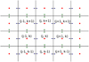Fig. 1 Illustration of staggered grid. Scalar properties are defined at the locations of the red dots in the center of each cell. The x, R, r component of the velocity is located at the interfaces marked with blue arrows and the y, ɀ, θ component of the velocity is calculated at the interaces marked by green arrows. Counting is indicated by the index k in the vertical or polar direction and j in the horizontal or radial direction. The location of variables at cell centers is expressed with integer indices and at cell faces with the integer $\pm \frac{1}{2}$ notation.

2.3 Discretization and interpolation

For the spatial discretization, we distinguished between source terms and advective terms, and between variables defined at cell centers and at cell faces. In the following, we use the generic variable, q ∈ |ρ, ℰ, m, n, l|, as a placeholder, where m is the linear momentum in the x, R, and r direction (j direction) and n is the linear momentum in the y, ɀ, or θ direction (k direction). l is the angular momentum as defined in the previous section. We express the advective term as $$\begin{array}{l}{\mathbf{\nabla }\cdot (q\mathit{\upsilon })|}_{j,k}=\frac{u_{j+\frac{1}{2},k}{[q]}_{j+\frac{1}{2},k}-u_{j-\frac{1}{2},k}{[q]}_{j-\frac{1}{2},k}}{x_{j+\frac{1}{2},k}-x_{j-\frac{1}{2},k}}\\ +\frac{v_{j,k+\frac{1}{2}}{[q]}_{j,k+\frac{1}{2}}-v_{j,k-\frac{1}{2}}{[q]}_{j,k-\frac{1}{2}}}{y_{j,k+\frac{1}{2}}-y_{j,k-\frac{1}{2}}},\end{array}$$(7)

where ${[q]}_{j\pm \frac{1}{2},k}$ is the interpolated (upwinded) value of q to the respective interface between cells j and j ± 1. Equally, ${[q]}_{j,k\pm \frac{1}{2}}$ is the upwinded value of q to the interface between k and k + 1. The velocities, u and v, were computed from their linear momentum counterparts, obtained from the momentum equations as $$u_{j\pm \frac{1}{2},k}=\frac{m_{j\pm \frac{1}{2},k}}{{\overline{\rho }}_{j\pm \frac{1}{2},k}}\text{\hspace{1em} and \hspace{1em}}{v}_{j,k\pm \frac{1}{2}}=\frac{n_{j,k\pm \frac{1}{2}}}{{\overline{\rho }}_{j,k\pm \frac{1}{2}}}\text{, }$$(8)

where we used the directly known values of $m_{j\pm \frac{1}{2},k}\text{ and }{n}_{j,k\pm \frac{1}{2}}$ as well as the density values interpolated as $${\overline{\rho }}_{j\pm \frac{1}{2},k}=\frac{{\rho }_{j,k}+{\rho }_{j\pm 1,k}}{2}\text{\hspace{1em} and \hspace{1em}}{\overline{\rho }}_{j,k\pm \frac{1}{2}}=\frac{{\rho }_{j,k}+{\rho }_{j,k\pm 1}}{2}\text{. }$$(9)

In cylindrical coordinates, the advection term is $$\begin{array}{l}{\mathbf{\nabla }\cdot (q\mathit{\upsilon })|}_{j,k}=\frac{R_{j+\frac{1}{2},k}{u}_{j+\frac{1}{2},k}{[q]}_{j+\frac{1}{2},k}-R_{j-\frac{1}{2},k}{u}_{j-\frac{1}{2},k}{[q]}_{j-\frac{1}{2},k}}{\frac{1}{2}\left(R_{j+\frac{1}{2},k}^2-R_{j-\frac{1}{2},k}^2\right)}\\ +\frac{v_{j,k+\frac{1}{2}}{[q]}_{j,k+\frac{1}{2}}-v_{j,k-\frac{1}{2}}{[q]}_{j,k-\frac{1}{2}}}{z_{j,k+\frac{1}{2}}-z_{j,k-\frac{1}{2}}},\end{array}$$(10)

and in spherical coordinates (see e.g., Shadab et al. 2019, Wang & Johnsen 2017) $$\begin{array}{l}{\mathbf{\nabla }\cdot (q\mathit{\upsilon })|}_{j,k}=\frac{r_{j+\frac{1}{2},k}^2{u}_{j+\frac{1}{2},k}{[q]}_{j+\frac{1}{2},k}-r_{j-\frac{1}{2},k}^2{u}_{j-\frac{1}{2},k}{[q]}_{j-\frac{1}{2},k}}{\frac{1}{3}\left(r_{j+\frac{1}{2},k}^3-r_{j-\frac{1}{2},k}^3\right)}\\ +\frac{1}{r_{j,k}}\frac{r_{j,k+\frac{1}{2}}\cos {\theta }_{j,k+\frac{1}{2}}{v}_{j,k+\frac{1}{2}}{[q]}_{j,k+\frac{1}{2}}-r_{j,k-\frac{1}{2}}\cos {\theta }_{j,k-\frac{1}{2}}{v}_{j,k-\frac{1}{2}}{[q]}_{j,k-\frac{1}{2}}}{\sin {\theta }_{j,k+\frac{1}{2}}-\sin {\theta }_{j,k-\frac{1}{2}}}.\end{array}$$(11)

In the staggered grid approach, the cells for the momenta in the j and k directions are shifted half a cell in the respective direction and the advection equations take a slightly different form. For the momentum, m, in the j direction, we have in Cartesian coordinates $$\begin{array}{l}{\mathbf{\nabla }\cdot (m\mathit{\upsilon })|}_{j-\frac{1}{2},k}=\frac{{\overline{u}}_{j,k}{[m]}_{j,k}-{\overline{u}}_{j-1,k}{[m]}_{j-1,k}}{x_{j,k}-x_{j-1,k}}\\ +\frac{{\overline{v}}_{j-\frac{1}{2},k+\frac{1}{2}}{[m]}_{j-\frac{1}{2},k+\frac{1}{2}}-{\overline{v}}_{j-\frac{1}{2},k-\frac{1}{2}}{[m]}_{j-\frac{1}{2},k-\frac{1}{2}}}{y_{j-\frac{1}{2},k+\frac{1}{2}}-y_{j-\frac{1}{2},k-\frac{1}{2}}},\end{array}$$(12)

where the values of $\overline{u}\text{ and }\overline{\upsilon }$ are defined as $${\overline{u}}_{j,k}=\frac{1}{2}\frac{m_{j-\frac{1}{2},k}+m_{j+\frac{1}{2},k}}{{\rho }_{j,k}}\text{\hspace{1em} and }$$(13) $${\overline{v}}_{j-\frac{1}{2},k+\frac{1}{2}}=\frac{1}{2}\left[\frac{n_{j-1,k+\frac{1}{2}}}{\frac{1}{2}\left({\rho }_{j-1,k}+{\rho }_{j-1,k+1}\right)}+\frac{n_{j,k+\frac{1}{2}}}{\frac{1}{2}\left({\rho }_{j,k}+{\rho }_{j,k+1}\right)}\right]\text{. }$$(14)

The procedure for the momentum in the k direction is equivalent, as are the expressions in cylindrical and spherical coordinates.

The upwinding method is equivalent for scalar variables and momentum components. We implemented the constant interpolation and first-order-accurate donor cell (DC) scheme, $$q_{j-\frac{1}{2}}=\{\begin{array}{ll}{q}_{j-1}\hfill & ,{\upsilon }_{j-\frac{1}{2}}>0\hfill \\ q_j\hfill & ,{\upsilon }_{j-\frac{1}{2}}<0,\hfill \end{array}$$(15)

as well as the generalized upstream-biased κ scheme, $$\begin{array}{l}{q}_{j-\frac{1}{2}}=q_c+\underset{{\sigma }_{j-\frac{1}{2}}^{\kappa }}{\underbrace{\frac{1}{4}\left[(1-\kappa )\left(q_c-q_u\right)+(1+\kappa )\left(q_d-q_c\right)\right]}},\\ \left(q_d,q_c,q_u\right)=\{\begin{array}{ll}\left(q_j,q_{j-1},q_{j-2}\right),\hfill & v_{j-\frac{1}{2}}>0\hfill \\ \left(q_{j-1},q_j,q_{j+1}\right),\hfill & v_{j-\frac{1}{2}}<0,\hfill \end{array}\end{array}$$(16)

where, for example, for κ = −1 the second-order-accurate linear upwind scheme (LUS; Price et al. 1966) and for $\kappa =\frac{1}{2}$ the third-order-accurate quadratic upwind interpolation scheme (QUICK) (Leonard 1979), are recovered. ${\sigma }_{j-\frac{1}{2}}^K$ is the inferred slope at the $j-\frac{1}{2}$ interface.

The velocities for upwinding (v or u) are taken at the respective interfaces of the variable cells. It becomes obvious that one has to take care of the nonlinearities present, especially in the equations of momenta, since the condition for the direction in which upwinding is conducted is dependent on the result of the upwinding. We address this issue, as well as the general implicit solution procedure, in the next section. From the interpolation methods, Eqs. (15) and (16), only the DC scheme is total variation diminishing (TVD). To prevent the occurrence of spurious oscillations in the vicinity of discontinuities (see Sect. 4.2), we implemented various slope-limiters (see e.g., Zhang et al. 2015 and references therein) but used the superbee limiter throughout this work. The final flux at the left interface of a cell, j, is then given as $${[q]}_{j-\frac{1}{2}}=q_{j-\frac{1}{2}}^{DC}-\frac{1}{2}\text{Φ}\left(r_{j-\frac{1}{2}}\right)\left(q_{j-\frac{1}{2}}^{DC}-q_{j-\frac{1}{2}}^{k\text{-scheme }}\right)$$(17) $$=q_{j-\frac{1}{2}}^{DC}+\text{Φ}\left(r_{j-\frac{1}{2}}\right){\sigma }_{j-\frac{1}{2}}^K.$$(18)

The resulting flux, $f_{j-\frac{1}{2}}={[q]}_{j-\frac{1}{2}}{v}_{j-\frac{1}{2}}$, is given by the interpolated variable times the velocity at that position. The superbee limiter is given by $$\text{Φ}\left(r_{j-\frac{1}{2}}\right)=\max \left(0,\min \left(1,2r_{j-\frac{1}{2}}\right),\min \left(2,r_{j-\frac{1}{2}}\right)\right),$$(19)

with the ratio of successive gradients $$r_{j-\frac{1}{2}}=\frac{{\sigma }_{j-\frac{3}{2}}^K}{{\sigma }_{j-\frac{1}{2}}^K}.$$(20)

Usually one would express Eq. (18) as a function of the left state at an interface, $q_{j-\frac{1}{2}}^L$, and the corresponding right state at the same interface,$q_{j-\frac{1}{2}}^R\text{ as }{[q]}_{j-\frac{1}{2}}=f\left(q_{j-\frac{1}{2}}^L,q_{j-\frac{1}{2}}^R\right)$. The left and right states correspond in this notation to the upwinded and downwinded states at the interface. We omit the superscripts in Eq. (18) because we use either $q_{j-\frac{1}{2}}^L\text{ or }{q}_{j-\frac{1}{2}}^R$, depending on the direction of the flow, and never both at the same time such that ƒ (·, ·) itself is an upwinding operator. The obtained scheme is generally similar to the monotone upwind scheme for conservation laws (MUSCL; van Leer 1979) and equivalent for $\kappa =\frac{1}{2}$.

2.4 Time stepping

Temporal discretization is much simpler than spatial discretization, yet its implications are much more complicated. We implemented the first-order-accurate Euler scheme (BDF-1), $$\frac{\partial q}{\partial t}\Rightarrow \frac{q^{n+1}-q^n}{\text{Δ}t}$$(21)

and the second-order-accurate 3-4-1 Euler scheme (BDF-2; e.g., Hai 1993), $$\frac{\partial q}{\partial t}\Rightarrow \frac{3q^{n+1}-4q^n+q^{n-1}}{2\text{Δ}t}$$(22)

where the first time step of every simulation run is always carried out using the BDF-1 scheme. We implemented different modes for the time step size calculation. The first is an a priori configured constant time step and the second an exponentially growing time step, $$\text{Δ}{t}^{n+1}=\{\begin{array}{ll}\alpha \cdot \text{Δ}{t}^n,\hfill & \text{Δ}{t}^n\le \text{Δ}{t}_{\max }\hfill \\ \text{Δ}{t}^n\hfill & \text{ else }\hfill \end{array}$$(23)

with α being the growth factor, which we usually set as 1 < α < 1.1. The third option is a dynamic time step proposed by Dorfi (1997), where $$\text{Δ}{t}^{n+1}=\{\begin{array}{ll}\frac{1}{2}\text{Δ}{t}^n,\hfill & s>s_{\max }\hfill \\ \text{Δ}{t}^n,\hfill & \frac{1}{2}{s}_{\max }\le s\le s_{\mathrm{max },}\hfill \\ \frac{3}{2}\text{Δ}{t}^n,\hfill & s<\frac{1}{2}{s}_{\max }\hfill \end{array}$$(24)

with $$s=\frac{\left|{\mathit{x}}^{n+1}-{\mathit{x}}^n\right|}{\left|{\mathit{x}}^n\right|}$$(25)

and where xⁿ is the vector containing all variables at time step, n, and s_max ≈ 0.1, typically. As Δt⁰, we usually selected a time step that is Δt ~ 10²Δt_explicit of the explicit time step, defined via the speed of sound, or found one that is sufficient by trial and error. In addition, we opened up the possibility of limiting all time step sizes to a Courant number of one given by the advection velocity (CFL_adv), ignoring the condition imposed by the speed of sound (CFL_cs), since we noticed that too-large time steps increase the numerical diffusion in a similar way as small time steps do.

One has to note here that both Courant numbers are calculated by our code as $\text{CFL}=\frac{\max \left(u_{\max },v_{\max }\right)\text{Δ}t}{\text{Δ}x}$. The only way of distinguishing between CFL_cs and CFL_adv is the size of Δt itself. When Δt is such that $\frac{c_s\text{Δ}t}{\text{Δ}x}>1$, we observe the filtering of sound waves (Sect. 4.1) and the sound speed is not represented in max(u_max, υ_max) used by the code. We hence can be sure that we are using $$\text{CFL}=\{\begin{array}{ll}{\text{CFL}}_{\text{adv}}\hfill & \text{ if Δ}t>\text{Δ}{t}_{\text{explicit }}\hfill \\ {\text{CFL}}_{\text{cs}}\hfill & \text{ else}.\hfill \end{array}$$(26)

2.5 System construction

In the implicit method, we are solving the fluxes and source terms in dependence of the as-yet-unknown properties at the next time level, n + 1. For a single linear equation in 1D, this is straightforward; for example, the continuity equation in a semi-discrete form for a time-independent velocity vector is $${\rho }^{n+1}+\nabla \cdot \left({\rho }^{n+1}\mathit{\upsilon }\right)\text{Δ}t={\rho }^n(\text{ BDF-1) },$$(27) $$\frac{3}{2}{\rho }^{n+1}+\nabla \cdot \left({\rho }^{n+1}\mathit{\upsilon }\right)\text{Δ}t=\underset{\text{known }}{\underbrace{\frac{4}{2}{\rho }^n-\frac{1}{2}{\rho }^{n-1}}}\text{\hspace{1em} (BDF-2)}.$$(28)

When spatially discretized with the methods outlined in the previous section, we can utilize two different formulations for the fully discretized NSE. We can either formulate them in operator form for every cell, which we denote as $${ℒ}_{\rho }\left({\rho }^{n+1}\right)=\text{ rhs },$$(29)

or in the form of a linear system with the systems matrix, A_ρ, as $$A_{\rho }{\rho }^{n+1}=\text{ rhs ,}$$(30) $$\Rightarrow A_{\rho }=\alpha I+\text{Δ}t{B}_{\rho }\text{. }$$(31)

Here, I is the identity matrix and B_ρ is the matrix that is defined by the advection and source term and that depends on the utilized upwinding scheme. For the BDF-1 scheme, α = 1, and for BDF-2, $\alpha =\frac{3}{2}$. The subscript, ρ, indicates that the system represents the continuity equation. Although we used only the continuity equation as an example, equivalent formulations exist for the other equations in the operator form, 𝓛_ℰ, 𝓛_m, 𝓛_n, and 𝓛_l, as well as in the matrix form, A_ℰ, A_m, A_n, and A_l.

In the 1D case, the matrices, A_q, are tridiagonal for DC and pen-tadiagonal for LUD and QUICK, as one can easily verify looking at the stencil of the respective schemes. The 2D and 3D axisym-metric cases are more complicated, since one needs to decide the ordering of j and k when constructing the system matrix as well as the systems vector, 𝓛_q.

It makes sense to either order all j for every k or all k for every j. In both cases, far off-diagonal elements are introduced into the system matrices. Hujeirat & Rannacher (1998) used the first approach because of the radial dominance of the considered flows and the resulting advantage of keeping the radial coupling terms close to the main diagonal in their defect-correction-solution approach. Although this is of limited importance in our matrix-free approach, we chose the same ordering, since it is in our case advantageous to have larger coupling terms close to the main diagonal for one of the preconditioners that we implemented (see Sect. 3.3.2).

Further complexity arises from the need to solve multiple interdependent equations concurrently. Different strategies have been explored to tackle this challenge, including sequential approaches, where each equation is solved one after the other, and simultaneous approaches, where all of the equations are collectively formulated into a single system. Various combinations of these approaches have been investigated in prior work (Hujeirat 2005, Hujeirat & Rannacher 1998). Although our implementation allows for flexibility in incorporating different combinations of sequential and simultaneous parts, we focused exclusively on the fully simultaneous case where for each cell, represented by indices j and k, a vector of length N (the number of equations solved) was utilized to store the solved variables. For the NSE, the vector of a single cell is then $${\mathit{cell}}_{j,k}=\left(\begin{array}{l}{\rho }_{j,k}\hfill \\ {\mathit{ℰ}}_{j,k}\hfill \\ m_{j,k}\hfill \\ n_{j,k}\hfill \\ l_{j,k}\hfill \end{array}\right)\in {ℝ}^N,{\mathit{ℒ}}_{j,k}=\left(\begin{array}{l}{\mathit{ℒ}}_{\rho }{(\rho ,\mathit{ℰ},m,n,l)}_{j,k}\hfill \\ {\mathit{ℒ}}_{\mathit{ℰ}}{(\rho ,\mathit{ℰ},m,n,l)}_{j,k}\hfill \\ {\mathit{ℒ}}_m{(\rho ,\mathit{ℰ},m,n,l)}_{j,k}\hfill \\ {\mathit{ℒ}}_n{(\rho ,\mathit{ℰ},m,n,l)}_{j,k}\hfill \\ {\mathit{ℒ}}_l{(\rho ,\mathit{ℰ},m,n,l)}_{j,k}\hfill \end{array}\right).$$(32)

This fills K lines, each of length J, as $${\mathit{line }}_k=\left(\begin{array}{c}{\text{ cell }}_{0,k}\\ {\text{ cell }}_{1,k}\\ \dots \\ {\text{ cell }}_{J-2,k}\\ {\text{ cell }}_{J-1,k}\end{array}\right)\in {ℝ}^{N\times J},{\mathit{ℒ}}_k=\left(\begin{array}{c}{\mathit{ℒ}}_{0,k}\\ {\mathit{ℒ}}_{1,k}\\ \dots \\ {\mathit{ℒ}}_{J-2,k}\\ {\mathit{ℒ}}_{J-1,k}\end{array}\right),$$(33)

which in turn make up the final systems vector, $$\mathit{x}=\left(\begin{array}{c}{\text{ line }}_0\\ {\text{ line }}_1\\ \cdots \\ {\text{ line }}_{K-2}\\ {\text{ line }}_{K-1}\end{array}\right)\in {ℝ}^{N\times J\times K},\mathit{ℒ}=\left(\begin{array}{c}{\mathit{ℒ}}_0\\ {\mathit{ℒ}}_1\\ \cdots \\ {\mathit{ℒ}}_{K-2}\\ {\mathit{ℒ}}_{K-1}\end{array}\right)$$(34)

The consequence of such a multivariate systems vector with coupled variables is that the structure of the systems matrix changes from a line-diagonal matrix to a block-diagonal matrix, because for every cell (j, k) there now exists an N × N block instead of a single entry. Since the goal of the code is to solve the NSE in an implicit way, we need to solve $$A\left({\mathit{x}}^{n+1}\right){\mathit{x}}^{n+1}={\mathit{x}}^n$$(35)

for xⁿ⁺¹. It is noteworthy at this point that the arising system is very sparse, contains far off-diagonal elements, is non-symmetric, nonlinear, and not necessarily positive-definite or diagonally dominant, but also non-singular and diagonalizable in real space (hyperbolicity of the NSE). These properties make it a) possible to solve the system and b) particularly difficult to do so in an efficient way.

One may notice that we introduced the construction for the system matrix instead of for the Jacobian matrix of the system. We did this because the definition of the system matrix is more intuitive and with the definition $A=\frac{\partial {ℒ}_q}{\partial x}\text{ and }J=\frac{\partial \left({ℒ}_q-\text{rhs}\right)}{\partial x}$ the matrices are equivalent. In the following, we rely only on the Jacobian matrix, as is outlined below.

3 Solution procedure

To solve the large, sparse, and nonlinear system mentioned above, one needs to linearize the system first (Eq. (36)) by using a kind of Newtons method or a defect-correction approach (e.g., Auzinger 1987) or by employing a dedicated method for nonlinear systems like, for example, the full approximation scheme (FAS) based on the multigrid method (see e.g., Henson 2003). We chose the more traditional approach of linearizing the system first and then applying a linear solver iteratively to obtain a solution. In the following section, we briefly describe our overall solution method before we go into detail on the different modules incorporated.

3.1 General approach

We started by linearizing the system, summarizing all NSEs on the complete solution domain in Eq. (35) with the Newtons method. In this approach, the Jacobian matrix of the residual function for the system is utilized to calculate approximations to the solution vector of the system. Except for the nonlinearity, the other properties – especially the sparsity and invertability – of the system matrix are inherited by the Jacobian matrix. To ensure distinguishability, we refer to the nonlinear system in the operator form as 𝓛 and to the linearized version as L. By linearized, we refer here to the fact that in the advection term of the momentum equations we made the transition (in a semi-discrete form) $$\left({\mathit{m}}^{n+1}\otimes {\mathit{\upsilon }}^{n+1}\right)\Rightarrow \left({\mathit{m}}^i\otimes {\mathit{\upsilon }}^{i-1}\right),$$(36)

using i as the Newton iteration step index (see Sect. 3.2). Further, we distinguish between the nonlinear residual function, 𝓡 = 𝓛 − b, and the linearized residual function, R = L − b, where b is the right-hand-side vector (see Eq. (29)). The Jacobian, J_R, is always calculated from R.

Because of the large size and the high degree of sparsity of J_R, direct dense solution methods, such as for example Gauss elimination, are not feasible. Luckily, dedicated solution methods for sparse linear systems exist as direct methods (LU, QR, Cholesky, etc.), iterative methods (e.g., Jacobi, Gauss-Seidel, SOR, and Krylov methods), and multigrid methods (see Barrett et al. 1994). The first class of direct methods is only attractive in the 1D case where J_R is (block)-diagonal and only matrix elements close to the main diagonal exist. Since we are dealing with the more general 2D case where far-off diagonal elements also exist, we focus on iterative methods, especially Krylov subspace methods (Sects. 3.3.1 and 3.3.2). These methods find a solution iteratively by spanning for the residual function, r₀ = rhs − Ax₀, the Krylov subspace, 𝒦_m = {Ar₀,A²r₀,….,A^m−1r₀}, and hence only rely on matrix-vector products to find the solution, which is particularly practical because we can express the matrix vector product in operator form, as is described in Sect. 2.5. This allows for the solution of the linear system in a matrix-free way, which is not possible when incorporating the Jacobi or Gauss-Seidel methods – or any derivatives of them – since they explicitly rely on individual matrix components. It should be noted that by the term matrix-free, no reference to the internal storing scheme of matrix components is made. It means that no free standing matrix is calculated and information about the matrix is only present implicitly through the matrix-vector product.

At this point, we want to stress that the usage of a matrix-free approach is not only useful because it allows one to compute the matrix-vector product on the fly, and thus offers the possibility to save storage. In fact, we did not notice a huge difference in memory consumption in our implementation. The far more important aspect is that for the Newtons method it is advantageous to have as exact a Jacobian matrix-vector product as possible to guarantee good convergence behaviour, and hence calculate the Jacobian matrix exactly, too. This task is very difficult to achieve when the matrix is expressed by components and very easy to achieve when the matrix-vector product is approximated by a finite difference approach.

3.2 Newton’s method

Methods building on the Newton method for linearization and using a Krylov subspace method for the solution of the consecutive equation are called Newton-Krylov methods. The multivari-ate Newton method can be expressed as $$\begin{array}{l}{\mathit{x}}^{i+1}={\mathit{x}}^i+{\left[\frac{\partial {\mathit{R}}^i}{\partial {\mathit{x}}^i}\right]}^{-1}\cdot {\mathit{ℛ}}^i\\ ={\mathit{x}}^i+\underset{\mu }{\underbrace{{\left[J_{\text{R}}\left({\mathit{x}}^i\right)\right]}^{-1}\cdot {\mathit{ℛ}}^i}},\end{array}$$(37)

where µ is the correction per iteration step and i is the iteration step. Dropping the superscript i, the linear system to be solved once per Newton iteration step is then $$J_{{\text{R}}^i}(\mathit{x})\mu =\mathit{ℛ}\equiv \mathit{ℒ}(\mathit{x})-b.$$(38)

The need for the calculation of the Jacobi matrix here is quite obvious. The calculation can be done in three different ways, with the first being manually calculating the coefficients and writing them in a sparse matrix. This can be computationally extremely fast but comes at the cost of the manual determination of each nonzero matrix element, making the development difficult and the approach much less flexible. The second approach is automatic differentiation, which is also relatively fast but which requires intimate knowledge of the sparsity pattern of the resulting matrix and imposes some implementation constraints. Both approaches have the disadvantage of having to store the complete and exact Jacobian matrix with all its elements but at the same time the advantage of being able to make use of efficient point methods.

The third method is the finite difference method, which requires the storage of only a single vector, as opposed to individual matrix elements. In this method, the Jacobian cannot be calculated as a stand-alone but only as a matrix-vector product, J_Rx. This is both an advantage, since it allows for a matrix-free solution procedure with a Krylov solver – which is less memory intense, easier to compute, faster, and easier to parallelize than other approaches – and a disadvantage, since it prohibits the use of methods requiring single elements of the matrix like, for example, Jacobi, Gauss-Seidel, and SOR, etc. The biggest advantage of the finite difference method is that the Jacobian matrix-vector product can be approximated to good accuracy without much effort.

Overall, we see the highest potential in using the finite difference approach with which we can write the first-order matrix-free vector product in dependence on the linearized operator, L, as $$J_{{\text{R}}^i}\left({\mathit{x}}^i\right)\mathit{\mu }=\frac{L\left({\mathit{x}}^i+{ϵ}_m\mathit{\mu },{\mathit{x}}^{i-1}\right)-L\left({\mathit{x}}^i,{\mathit{x}}^{i-1}\right)}{{ϵ}_m}$$(39)

using the machine-precision epsilon, ϵ_m. Strictly speaking, this formulation yields Broyden’s method (the secant method) for finite ϵ, but when solved to machine precision, both methods are equivalent in practice. The difficulty is to find the correction, µ, by iteratively finding a solution to the inversion problem, $$\frac{L\left({\mathit{x}}^i+{ϵ}_m\mathit{\mu }\right)-L\left({\mathit{x}}^i\right)}{{ϵ}_m}=\mathit{ℒ}\left({\mathit{x}}^i\right)-\mathit{b}$$(40) $$\iff \mathit{\mu }=\frac{L^{-1}\left[{ϵ}_m\cdot \left(\mathit{ℒ}\left({\mathit{x}}^i\right)-\mathit{b}\right)+L\left({\mathit{x}}^i\right)\right]-{\mathit{x}}^i}{{ϵ}_m}.$$(41)

In the following section, we describe methods of finding solutions for µ.

We note that the term matrix-free does not merely refer to an implementation detail of the method in terms of programming. In applied mathematics, this term refers to the fact the desired matrix-vector product is evaluated through a vector-valued function rather than a matrix-vector multiplication, and thus describes the method itself. In our case, this function is given by the right-hand side in Eq. (39), while the left-hand side in that equation describes the matrix-based method. In our method, xⁱ⁻¹ and xⁱ, and consequently the result of L(xⁱ, xⁱ⁻¹), are fixed points calculated once per Newton iteration step. L(xⁱ + ϵ_mµ, xⁱ⁻¹) is evaluated multiple times in every Newton step to find µ such that Eq. (40) is satisfied (see Sect. 3.3). In a matrix-based method, the equivalent to this form of updating would be to recalculate the Jacobian matrix after every linear solver iteration step, based on the value of the last iterate. In matrix-free methods, this approach is included by construction, and all variables and interpolations described in Sect. 2.3 are evaluated at the most recent linear-solver step of the most recent Newton iteration step. In this respect, matrix-based methods are more flexible, since they allow the Jacobian matrix to be evaluated once per linear solver step (equivalent to our approach), once per Newton step (the Newton-Raphson method), or even only once per time step (yielding a defect-correction approach). We sacrificed this flexibility in order not to be dependent on the expensive and difficult construction of the Jacobian matrix.

Independent of its matrix-free or matrix-based formulation, Newton’s method is based on an updating step, as is given by Eq. (37), and may not converge for nonlinear problems using large advective Courant numbers (e.g., CFL_adv ≳ 2 for the Sod’s shock tube in Sect. 4.2). To counter this, we implemented the possibility of using damping (e.g., Nowak & Weimann 1992), where instead of Eq. (37), the update is performed as $${\mathit{x}}^{i+1}={\mathit{x}}^i+{\lambda }_{\text{damp }}\mathit{\mu }\text{, }$$(42)

where 0 < λ_damp ≤ 1 is the damping factor. µ was calculated without change to the undamped case using Eq. (41).

3.3 Solvers

Since we defined Eq. (39) in a matrix-free way, a matrix-free solver was needed to solve for µ. The only possibilities were either to use an appropriate Krylov subspace method directly or a geometric method (meaning domain decomposition and geometric multigrid methods) built around one. In the following, we give a brief and very qualitative overview of the solvers that we implemented, in which our goal is to present the possible options for a solution pathway instead of giving a detailed description of every individual solver. For this, the reader is referred to Saad (2003) and references within as well as to the individual references within the section.

3.3.1 Krylov methods

Krylov subspace methods obtain a solution by iteratively evaluating matrix-vector products and consequently spanning a Krylov subspace. A popular and very efficient choice for elliptical problems is the conjugate gradient (CG) method, which we unfortunately cannot use because it is valid only for symmetric and positive-definite systems, which for the hyperbolic system we are dealing with is not the case. For the more general nonsymmetric and not necessarily positive-definite hyperbolic system we are dealing with, biconjugate gradient stabilization (BiCGSTAB) or the generalized method of residuals (GMRES) can be applied (Saad & Schultz 1986).

Although BiCGSTAB has a small scaling factor, it makes use of two matrix-vector calculations per iteration as opposed to GMRES, which has a scaling factor that grows with the number of iterations but makes use of only one matrix-vector product per iteration. Additionally, convergence is not guaranteed for BiCGSTAB, while for a system of size N × N GMRES becomes a direct method after N iterations and monotonic convergence is guaranteed (see Saad 2003 for details). We implemented both methods and oriented our implementations on the work by Guennebaud et al. (2010) in the C++ eigen package.

It is a well-known fact that convergence of both methods can be accelerated a great deal in terms of necessary iterations and numerical stability by using a suitable precondi-tioner (van der Vorst 2003, Pearson & Pestana 2020). Because GMRES only needs one matrix-vector product, and hence one preconditioning cycle per iteration, and has guaranteed convergence, we focus on the usage of GMRES in the following. We implemented a matrix-free, correctly preconditioned version of restarted GMRES, making use of Eq. (39) and paying attention to the flexibility of using different preconditioners.

3.3.2 Preconditioners

One of the implemented and most-used preconditioners was ILUT, in which we calculated the required matrix coefficients only approximately by hand a priori and only once per Newton iteration step. We followed the philosophy here that an exact Jacobian matrix in components is difficult to compute and an approximation of it is easy to find, which from our experience is indeed the case. To compute the matrix components for ILUT, we treated the derivatives in the viscous terms especially loosely and always approximated the derivatives from the advection terms as if they would arise from the DC scheme.

The most important components that should be recovered rather exactly are the diagonal entries arising from the time derivative since they ensure non-singularity of the matrix and the pressure gradient term. The latter was incorporated into the Jacobian matrix through the equation of state. Despite its great acceleration properties, there are two main drawbacks to the usage of ILUT. The first is its inherent sequentiality when computed, which for larger systems becomes an obvious issue. The second drawback is its dependence on individual components of the Jacobian matrix that make a complete matrix-free operation mode impossible and reduce the flexibility of our solver a great deal.

To prohibit this, we also implemented operation modes of GMRES and BiCGSTAB without preconditioning (an identity preconditioner) and with an approximate Jacobian precondi-tioner where only the advection term of each equation was considered and advection was treated as if it was done by first-order upwinding. In this case, the complete preconditioner becomes a prefactor $\frac{1}{1+\frac{\text{Δ}t}{\text{Δ}x}\left|v_{x,jk}\right|+\frac{\text{Δ}t}{\text{Δ}y}\left|v_{y,jk}\right|}$. Although this preconditioner reduces the GMRES iterations in our test cases by only about 10%, its low computational cost justifies its usage nevertheless.

Although there exists a variety of more dedicated matrix-free preconditioners such as polynomial preconditioners (see e.g., Choquet 1995) or multigrid preconditioners (Hackbusch 1985, Bastian et al. 2019), their implementation is beyond the scope of this paper and will be the subject of future work.

3.4 Boundary conditions

The most common choices for boundary conditions (BCs) in astrophysics are periodic, reflective, and inflow or outflow boundaries as well as, sometimes, constant boundaries. In our implementation of all of these types of boundaries, each boundary consists of two cells to model; for example, inflow problems to the second order.

The representation of our boundary scheme in the x or radial direction is shown in Fig. 2 for the inner (left) and outer (right) ends of the simulation domain. The blue arrows indicate velocities belonging to the boundary cells and the black ones those to the outermost domain cell. The vertical arrows represent the vertical velocity components and the horizontal ones the radial components. The boundary scheme in the k direction is equivalent, with the only difference being the rotation of 90° counterclockwise and the change of the vertical arrows to the other end of the respective cell.

We do not give a detailed description of every type of BC but mention a few peculiarities about the implementation of BCs with implicit methods that apply likewise to Dirichlet and von Neumann BCs. The first is the treatment of the innermost velocity component of the domain represented by the horizontal black arrow on the left-hand side of Fig. 2. For reflective BCs, this value is kept zero at all times despite being inside the solution domain. There are three ways to deal with this. The first is to regularly solve the whole domain, as is described in Sect. 3.2, and to overwrite the value at every boundary update. The second option is to take the component out of the solution procedure and, for example, drop the respective index from Eq. (41) altogether. The third option is to keep the component but set the value of µ_BC to zero and $x_{\text{BC}}^{i+1}=x_{\text{BC}}^i$ for all time steps, thus keeping the velocity value constant to the initial value.

The first option has proven in our experience to decrease the stability of the solution method substantially, since it causes a decoupling of the used value for the boundary velocity from the solved one. The second option is technically difficult to implement and neglects the coupling to the boundary velocity, which also destabilizes the solution procedure. The third method does not come with these disadvantages, since on the one hand the velocity is kept constant as a result of the solution procedure itself and coupling to the boundary velocity is included. A more detailed description of this approach can be found, for example, in Keil (2010).

An additional difficulty is the positioning of the boundary update in the solution procedure. One can update the boundaries once after every time step, once after every Newton iteration step, or once after every linear solver step (GMRES or BiCGSTAB iteration step). For a qualified choice, not only computational cost has to be considered. In the cases where not only the domain values depend on the BCs but also the BCs depend on the domain values – as is the case for reflective BCs – an additional cross dependency is introduced to the solution method when the BCs are updated inside the Newton or the linear solver steps, which in principle has to be resolved through an additional iteration loop. In practice, we observed this to not be necessary, and we also did not observe a noticeable difference in computational speed but very much so in the consequent stability of the solver. Because of this, the BC update was done inside every linear solver step.

Furthermore, one has to consider the dependence on the upwinding procedure on the BCs. While the DC scheme requires information only from one boundary cell, LUD and QUICK would require two boundary cells when the flow comes out of the boundary. To still be able to use only one boundary cell, we fall back to the DC scheme in the direct vicinity of the boundary cells. Lastly, the incorporation of the BCs in the Jacobian matrix is essential. In our realization through the finite difference approximation and boundary update inside the linear solver step, this is already included. For matrix-based methods, this is not the case and can cause substantial numerical limitations if not done correctly. In principle, we are required to consider boundary effects when ILUT is utilized and matrix components are computed, but we found in practice that we can neglect them when the Courant number of the flow is not too large.

To summarize this section, a visual representation of the main steps and loops of the MATRICS solver routine is given in Fig. 3. The expression “Update Reference Jacobian” in step 12 describes the process of updating the vector, L(xⁱ, xⁱ⁻¹), in Eq. (39). Similarly, step 9, “Update Jacobian Matrix-Vector Product”, is equivalent to the evaluation of the full right-hand side expression in Eq. (39). This requires the preceding update of xⁱ⁺¹ = ϵ_mµ, making an additional variable update inside the Newton iteration step superfluous.

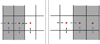Fig. 2 Boundary (gray) cells and the last cell in the domain in the respective direction for opposite sides of the domain. This depiction is equivalently valid in Cartesian, cylindrical, and spherical coordinates in both the j and k directions. The blue arrows indicate the position of velocities belonging to the boundary cells, and the black arrows those belonging to the outermost domain cell.

4 Test problems

We conducted test cases for every component of our code where in Cartesian coordinates we performed 1D tests to 1) illustrate the code’s ability to resolve sound waves when the chosen Courant number is sufficiently small and to average the waves out when a higher time step is chosen and 2) to show that we can reproduce analytic results for a physical problem. For the latter, we chose the well-studied shock tube problem by Sod (1978) where our focus is not on demonstrating shock-capturing capabilities of the numerical method but on demonstrating the code’s capability to model high-Mach-number flows.

To test our implementation of viscosity and the equations in cylindrical coordinates in 3D axisymmetry, as well as our boundary scheme, we simulated the flow between two rotating concentric cylinders known as the Taylor–Couette flow, for which analytic studies describing the onset of instability exist. With the reproduction of the analytic results, we proved the accuracy of the aforementioned components. The implementation in spherical coordinates alongside the implementation of gravity was tested with simulations of the vertical shear instability (VSI) where we reproduced growth rates obtained by Manger et al. (2020).

4.1 Propagating sound wave

We started by testing the compressible 1D Euler equations in Cartesian coordinates, considering thermal energy only using the caloric equation of state $$P=(\gamma -1)ℰ=(\gamma -1)\rho e\text{, }$$(43)

for an ideal gas with γ = 1.4 and specific internal energy, e. We chose a constant density profile, $\overline{\rho }=1$, which is distorted by a small amplitude sinusoidal profile, ${\rho }_0^{\prime }(x)={10}^{-4}$ • sin(x), giving ${\rho }_0(x)=\overline{\rho }+{\rho }_0^{\prime }(x)$ as an initial condition for density. In the adiabatic case, density and pressure are related via $$P=K{\rho }^{\gamma },$$(44)

where we set the constant, K = 1. From Eqs. (43) and (44), we calculated the specific internal energy and initialized the internal energy, ℰ₀(x) = ρ₀(x)e₀(x). With the adiabatic speed of sound, $c_s=\sqrt{\gamma \frac{P}{\rho }}=\sqrt{\gamma (\gamma -1)e}$, we obtained the initial fluid velocity for the sound wave and closed the set of initial conditions with the momentum, $$m_0(x)=c_{s,0}(x)\cdot {\rho }_0(x).$$(45)

We applied periodic BCs and set the integration domain to x ∈ [0,2π) with 100 grid points. We solved the continuity, momentum, and energy equations simultaneously and tested different time steps, and hence different CFL numbers. In Fig. 4, we show the time evolution of the density amplitude for different CFL numbers where we used the LUD scheme for spatial and the BDF-1 scheme for temporal integration solving with ILUT preconditioned GMRES restarted after 20 iterations.

The first features that one may notice are the sinusoidal oscillations present, which are small in amplitude and which can be explained with the setup of our initial conditions, where we made use of Eq. (45) to calculate momentum at $x_{j-\frac{1}{2}}=\frac{x_j+x_{j-1}}{2}$, but in the code we used $m\left(x_{j-\frac{1}{2}}\right)=\frac{m\left(x_j\right)+m\left(x_j-1\right)}{2}\ne m\left(\frac{x_j+x_{j-1}}{2}\right)$. One can work out the difference in momentum easily and obtain 𝓞(m_0,ics − m_0,code) = 10⁻⁵, which is in perfect agreement with the order of the oscillations observed here.

The noteworthy phenomenons are the overall trends observable for the different CFL numbers where for the CFL< 1 cases, the diminishing in the density fluctuation is linear and can be explained by the inherent and expected dissipation of the utilized upwinding scheme. The decrease is clearly superlinear for the CFL> 1, where the averaging out of the fluctuations for CFL ≈ 12 is reached faster than for CFL ≈ 1.2. In Fig. 5, the density fluctuations are plotted at t = 50, where the averaging-out of the density fluctuations is even more obvious.

With this, we proved our code’s capability to resolve sound waves when the chosen Courant number is smaller than one, and also its ability to operate in the CFL> 1 regime, where sound waves are averaged out with time in dependence of the time step size.

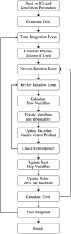Fig. 3 Schematic depiction of the main steps taken in the solution procedure of MATRICS.

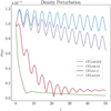Fig. 4 Evolution of the density perturbation in the sound wave test for different CFL numbers using 100 grid points, solving with the LUD and BDF-1 schemes.

4.2 Sod’s shock tube

Although shock modeling is not our primary concern, shocks can be used as a stress test to illustrate the limitations of our code. Sod’s shock tube problem (SSTP) is a well-studied problem with a known analytic solution (here taken from Toro 2009). Since a shock is by definition a high-Mach-number flow, kinetic energy cannot be neglected relative to thermal energy and has to be included in the energy equation as $$\frac{\partial {\mathit{ℰ}}^{\text{total }}}{\partial t}+\mathbf{\nabla }\cdot \left({\mathbf{ℰ}}^{\text{total }}\mathit{\upsilon }\right)=-(P\mathbf{\nabla }\cdot \mathit{\upsilon }+\mathit{\upsilon }\cdot (\mathbf{\nabla }P))$$(46)

where the total energy is ${ℰ}^{\text{total }}=ℰ+\frac{\rho }{2}\mathit{\upsilon }\cdot \mathit{\upsilon }$, giving the ideal gas equation of state for compressible flows, $$P=\left({ℰ}^{\text{total }}-\frac{1}{2}\rho \mathit{\upsilon }\cdot \mathit{\upsilon }\right)(\gamma -1)\text{. }$$(47)

Reconstruction of the quadratic velocity term was done in accordance with Eq. (36) as $$\begin{array}{l}\mathit{\upsilon }\cdot \mathit{\upsilon }\to \frac{u_{j-\frac{1}{2},k}^i+u_{j+\frac{1}{2},k}^i}{2}\frac{u_{j-\frac{1}{2},k}^{i-1}+u_{j+\frac{1}{2},k}^{i-1}}{2}\\ +\frac{v_{j,k-\frac{1}{2}}^i+v_{j,k+\frac{1}{2}}^i}{2}\frac{v_{j,k-\frac{1}{2}}^{i-1}+v_{j,k+\frac{1}{2}}^{i-1}}{2}\\ +w_{j,k}^i{w}_{j,k}^{i-1},\end{array}$$(48)

where i refers to the current Newton iteration step and i − 1 to the previous one. υ is the velocity in the vertical direction and ω the velocity perpendicular to the simulation plane. In this case of a 1D problem, only the first component (velocity u in the x direction) was considered. The difference between the total equation of state and the thermal equation of state used to model the SSTP can be seen in Fig. 6, from which it becomes obvious that the kinetic term cannot be neglected when no other entropy-generating terms such as von Neumann-Richtmyer (Landshoff) viscosity (VonNeumann & Richtmyer 1950, Landshoff 1955) are employed.

The initial conditions for the SSTP for density, thermal energy, and momentum on the domain, x ∈ [0, 1], were $$\rho (x,0)=\{\begin{array}{ll}1.0,\hfill & x<=0.5\hfill \\ 0.125,\hfill & x>0.5\hfill \end{array},$$(49) $${ℰ}^{\text{total }}(x,0)=\{\begin{array}{ll}\frac{1.0}{\gamma -1},\hfill & x<=0.5\hfill \\ \frac{0.1}{\gamma -1},\hfill & x>0.5\hfill \end{array},$$(50) $$m_x(x,0)=0.$$(51)

We solved the Euler equations with the equation of state in Eq. (47) and γ = 1.4, integrated to t = 0.2 using the BDF-1 scheme. The comparison for internal energy and velocity between the non-slope-limited QUICK, the slope-limited QUICK, and the DC schemes is shown in Fig. 7, where for reference the analytic solution from Toro (2009) is also shown.

With the fully simultaneous implicit approach we were able to model the SSTP with Courant numbers > 1, as we show in Fig. 8 for simulations with slope-limited QUICK using Courant numbers of up to four. 1000 domain cells were used in all cases. The cases with CFL numbers below two were solved using the standard Newton method and the CFL=4 case was obtained using Newton’s method with a damping factor of ${\lambda }_{\text{damp }}=\frac{1}{2}$.On the one hand, the choice of λ_damp < 1 extends the convergence radius of Newton’s method, but on the other hand can result in a higher number of iterations needed for convergence. It can be seen in Fig. 8 that as a function of Courant number, the numerical diffusion of the numerical scheme grows. This effect becomes especially prominent beyond CFL_adv > 1, indicating that this is a reasonable constraint to self-impose.

This becomes even more obvious when looking at Fig. 9, where instead of QUICK we used the DC scheme and an otherwise equal setup to reach a higher Courant number of CFL_adv = 14.5. The stronger diffusion compared to the smaller Courant number can clearly be seen and is also present for more dedicated shock-capturing methods, as for example in Fig. 6 by Fraysse & Saurel (2019), where a ten-times-higher spatial resolution was used with different time step sizes. The effect appears to be the same as for sound waves, meaning that not only sound waves are averaged out when CFL_cs > 1 but also macroscopic flows when CFL_adv > 1. We thus imposed the condition CFL_adv ≤ 1 on all our following runs.

An order evaluation of the slope-limited schemes is given in Table 1 using the average of the L₁ loss function over the whole domain as a measure of the spatial error. For the density, this average is defined as $$\langle L_1(\rho )\rangle =\frac{1}{N_x}{\displaystyle \sum _0^{N_x}\left|\left({\rho }_{\text{Simulated }}-{\rho }_{\text{Analytic }}\right)\right|},$$(52)

where N_x is the count of cells. The obtained slope in the log-log-space is with ~ − 1.7 close to minus two, as one would expect for the combination of the respective schemes and the superbee limiter, but due to the first-order component at the discontinuity not quite −2. We also show the solution to Sod’s shock using the same initial conditions – except a shift by 0.5 in the positive R direction – integrated using a spherical coordinate system in Fig. 10 in 3D axisymmetry for density and in Fig. 11 in the radial direction only for density, velocity, and pressure. The results for density, velocity, and pressure are very similar to those obtained by Balsara et al. (2020), who used a spherical geodesic mesh to model the problem, and to those of Omang et al. (2006), who solved the problem using a Lagrangian method.

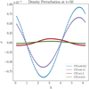Fig. 5 Density perturbation at t = 50 in code units for the sound wave test where time integration was done at different CFL numbers. The simulation was done with 100 cells, second-order upwinding, BDF-1 time integration, and periodic BCs.

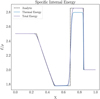Fig. 6 Comparison of the specific internal energy using total energy and thermal energy in the SSTP. 1000 grid cells were used and integration was done using the QUICK and BDF-1 schemes at a CFL number of ~0.5, where GMRES with ILUT preconditioning was used as solver.

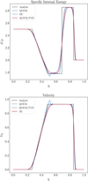Fig. 7 Specific internal energy (top) and velocity (bottom) for SSTP with 200 grid cells at time t = 0.2, integrated with BDF-1. The spatial scheme is indicated in the legend.

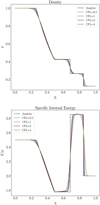Fig. 8 Density and specific internal energy of SSTP with 1000 grid cells at time t = 0.2, integrated with backward Euler and different CFL numbers. The slope-limited version of QUICK was used.

4.3 Taylor–Couette flow

TC is the flow between two concentric and independently rotating cylinders. It is generally characterized by the radius ratio, $\eta =\frac{r_{\text{i}}}{r_{\text{o}}}$, the gap width, d = r_o − r_i, as well as the Reynolds numbers, $R{e}_{\text{i}/\text{o}}=\frac{{\text{Ω}}_{\text{i}/0}{r}_{\text{i}/\text{o}}d}{v}$, and aspect ratio, $\text{Γ}=\frac{h}{d}$, for the height of the simulation domain, h, as well as the inner radius, r_i, and outer radius, r_o, respectively. Based on these properties, Andereck et al. (1986) describe different flow regimes where the laminar base flow (Couette flow) has the well-known analytical solution $$\begin{array}{c}{v}_{\theta }(r)=A\cdot r+\frac{B}{r},\\ A={\text{Ω}}_{\text{i}}\frac{{\text{Ω}}_{\text{o}}/{\text{Ω}}_{\text{i}}-{\eta }^2}{1-{\eta }^2},\\ B={\text{Ω}}_{\text{i}}{r}_{\text{i}}^2\frac{1-{\text{Ω}}_{\text{o}}/{\text{Ω}}_{\text{i}}}{1-{\eta }^2}.\end{array}$$(53)

The transition from Couette to Taylor vortex flow is dependent on the rotation relation between the inner and outer cylinders. In the case of a stationary outer cylinder, Rayleigh’s criterion is violated and the stability of the flow depends on the stabilizing effect of viscosity, which is usually expressed in terms of the Reynolds number. Since the original expression derived by Taylor (1923) (Schrimpf et al. 2021) of the critical Reynolds number (Re_crit) in the small gap limit, $$R{e}_{\text{crit }}=41.2\cdot \sqrt{\frac{\eta }{1-\eta }},$$(54)

many other approximations of the Taylor number as a stability criterion have been calculated and/or experimentally obtained (e.g., by Snyder 1968, Recktenwald et al. 1993, and Esser & Grossmann 1996) for different radius ratios. The aim of our test here was to reproduce the critical Reynolds numbers found in the literature to verify our implementation of axisymmetric cylindrical coordinates using viscosity and centrifugal terms, employing reflective and periodic BCs. For simplicity, we fixed the inner radius to r_i = 1 and the kinematic viscosity to v = 10⁻³ in code units. We kept the wall of the outer cylinder at rest (Ω_o = 0) and varied only the rotation, Ω_i, of the inner cylinder.

As initial conditions, we set the angular momentum according to Eq. (53) and the other momentum components to zero plus a small random fluctuation ~𝒪(10⁻⁵). From the equilibrium of pressure and centrifugal forces, $$\rho \frac{{\upsilon }_{\theta }^2}{r}=-\nabla P,$$(55)

together with the thermal equation of state (43), we solved for the specific internal energy, e = e(r), with the density set to ρ = ρ₀ = 1 and obtained $$e(r)=C_1+\frac{\frac{A^2{r}^2}{2}+2AB\log (r)-\frac{B^2}{2r^2}}{\gamma -1},$$(56)

with γ = 1.4. We chose C₁ = 10⁵ to obtain weak compressibility. This marks a difference to the theoretical descriptions, which assume full incompressibility, but from our experiments we observe density fluctuations in the order of the numerical accuracy we set (10⁻⁸) of the initial value of unity and no quantitative difference when compressibility is reduced through an increase in the initial specific internal energy, or even when the continuity equation is deactivated altogether.

We enforced reflective boundaries in the radial direction, where we kept Ω_i, and hence υ_φ,i fixed and solved the NSEs Eqs. (1) and (2), combined with the energy Eq. (4), ignoring viscous heating. We note that the problem can be modeled isothermally and the use of an energy equation is not mandatory. We included it here only for testing purposes. In the vertical direction, we chose periodic BCs, which seem to us most suited to model the case of an infinitely long cylinder, as we aim to do. We chose an aspect ratio, Γ = 4, giving a cell aspect ratio of Γ_cell = 2 and a radius ratio of η = 0.5, and conducted simulations with resolutions 20 × 40, 50 × 100, 100 × 200 and 200 × 400, to find a good compromise between accuracy and computational time to conduct further runs with.

Following Recktenwald et al. (1993), the onset of instability for the chosen radius ratio can be expected with Ω_in ≈ 0.68, corresponding to Re_crit ≈ 68. We chose a slightly larger value of Ω_i = 0.1 and used a time step of ∆t = 0.2 such that it can be used for all runs at CFL_adv < 1, which, depending on the resolution, is 10⁴–10⁶ that of the CFL number one would obtain when considering the sound speed. Time integration was done using BDF-2 and spatial integration using the QUICK scheme. We show typical results for the contours of the pressure, density, and the momentum components for this configuration in Fig. 12, where pressure and density have roughly the same shape. The difference is due to the fact that the GMRES accuracy was chosen to be 10⁻⁸, and hence in the order of the observed density changes.

In Fig. 13, we show the temporal evolution of the maximal velocity inside the domain to t = 1.5τ_vis of the viscous timescale, ${\tau }_{\text{vis}}=\frac{d}{v}$. One can clearly see the steep growth for all resolutions starting at 0.4τ_vis < t < 0.75τ_vis, with the lowest resolution starting slightly earlier. The growth phase is followed by a phase of relaxation at 0.75τ_vis < t < τ_vis and finally convergence to equilibrium at t > τ_vis. We saw the evolution tracks for the different resolutions converging relatively quickly, and thus decided to continue using the 50 × 100 resolution.

In Fig. 14, we tested different aspect ratios at the chosen radial resolution and cell aspect ratio of Γ_cell = 2. Once can again see the solution converging for larger aspect ratios, as was expected since we approach the case of an infinitely long cylinder. A clear outlier is the Γ = 2 case where not only the velocity growth sets in at a later time but also the observed overshoot shortly before relaxation is much higher. Both effects may be due to the supposedly uneven count of modes in the simulation domain. We conclude that a too-small domain aspect ratio as well as a too-small resolution artificially destabilize the flow and are not suited for our determination of the critical Reynolds number. Likewise, a larger domain aspect ratio with a higher resolution is computationally much more expensive.

As a compromise, the aspect ratio of Γ = 4 with a resolution of 50 × 100 seems sufficient for our main runs where we conducted for the radius ratios, η = {0.3,0.5,0.7,0.8,0.9,0.975}, multiple runs each to obtain the respective critical Reynolds number approximately through manual iterations. We obtain Re_crit for each radius ratio by choosing Ω_i in the vicinity of the value predicted by Recktenwald et al. (1993), integrating to t = 2τ_vis, and checking if considerable growth of the maximal velocity inside the domain can be observed. We increase or decrease Ω_i until we have one run where we have a largest Ω_i, where we see no growth and the smallest Ω_i where there is growth.

The results of our simulations are depicted in Fig. 15 where the theoretical predictions by Recktenwald et al. (1993) and Taylor (1923) are also plotted. The blue area is constrained by the criterion explained above. For the orange area, we chose a much smaller resolution of 20 × 40, integrated to t ≈ 1000τ_vis, and checked if the velocity inside the domain had vanished, which below the orange area is the case and inside it is not. The red crosses mark the radius ratios where we conducted our simulations.

As one can see, our runs with qualified guesses about the required resolution and aspect ratio to model the case of an infinitely long cylinder (blue) are in perfect agreement with theoretical predictions by Recktenwald et al. (1993) and for the gap width approaching the small gap limit also with those by Taylor (1923). As was expected from the first tests, the smaller resolution runs (orange) exhibit a more unstable behaviour while still being in agreement with theory.

Given the observed sensitivity of the test problem to small variations in viscosity, rotation, and chosen BCs, we conclude the accuracy of our implementations of the utilized physical terms.

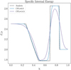Fig. 9 Specific internal energy density simulation of the SSTP with 1000 cells for two different CFL numbers. A total equation of state was used in both cases with first-order upwinding and the BDF-1 scheme. GMRES was selected as the solver.

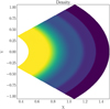Fig. 10 3D axisymmetric solution of Sod’s shock tube integrated in spherical coordinates to a dimensionless time of 0.2. 2002 cells and an advective CFL number of 0.5. The slope-limited QUICK scheme and the BDF-1 scheme were used. GMRES was selected as the solver.

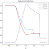Fig. 11 Solution of Sod’s shock tube integrated in spherical coordinates to a dimensionless time of 0.2. 200 cells and an advective CFL number of 0.5. The slope-limited QUICK scheme and the BDF-1 scheme were used. GMRES was selected as the solver.

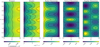Fig. 12 Contour lines of pressure, angular momentum, radial momentum, and vertical momentum together for the Taylor vortex flow after 1.5 viscous timescales. The plots were created from our test run with a resolution of 100 × 200 and an inner rotation of Ωi = 0.1 as well as the radius ratio, η = 0.5, and aspect ratio, Γ = 4, using periodic BCs in the vertical direction.

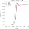Fig. 13 Temporal evolution of maximal velocity in the simulation domain for constant aspect ratio and different resolutions in the TC test problem. The QUICK and BDF-2 schemes were used and ILUT preconditioned GMRES was selected as the solver.

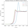Fig. 14 Temporal evolution of maximal velocity in the simulation domain for resolution and different aspect ratios in the TC test problem. The QUICK and BDF-2 schemes were used and ILUT preconditioned GMRES was selected as solver. The resolution was selected as 50 × 100.

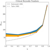Fig. 15 Experimentally derived ranges for the critical Reynolds numbers in the TC test problem for different radius ratios using high-resolution simulations to two viscous timescales (blue) and low-resolution simulations to 2000 viscous timescales (orange) in comparison to predictions by Recktenwald et al. (1993) (solid line) and Taylor (1923) (dotted line). The orange area marks the range where instability is obtained exclusively from the lower-resolution runs and no instability for the higher-resolution runs was found. The red crosses mark the position of the lowest value of the critical Reynolds number for the respective radius ratio that was obtained.

4.4 Vertical shear instability

The VSI (Urpin & Brandenburg 1998, Nelson et al. 2013) is believed to be a driver of turbulence in protoplanetary discs (PPDs), appearing in vertically stratified PPDs with a radial variation in its temperature profile and sufficiently short cooling time. For the modeling, initial conditions following Nelson et al. (2013) and Manger & Klahr (2018) were set up in equilibrium such that centrifugal forces exactly counter pressure and gravitational forces in the radial direction and pressure counters gravity in the vertical direction. The midplane (ɀ = 0) density and temperature are assumed to follow the radial profile $$\rho (R,Z=0)={\rho }_0{\left(\frac{R}{R_0}\right)}^p,$$(57) $$T(R,Z=0)=T_0{\left(\frac{R}{R_0}\right)}^q.$$(58)

Combining these equations with the balance of forces, one can work out the density and rotation profiles using the adiabatic pressure density relation, $P=c_s^2\rho$, to $$\rho (R,Z)={\rho }_0{\left(\frac{R}{R_0}\right)}^p\exp \left[\frac{GM}{c_s{(R)}^2}\left(\frac{1}{r}-\frac{1}{R}\right)\right],$$(59) $$\text{Ω}(R,Z)={\text{Ω}}_K(R){\left[1+q-\frac{qR}{r}+\frac{R{c}_s{(R)}^2\cdot (q+p)}{GM}\right]}^{1/2},$$(60)

with Keplerian rotation, ${\text{Ω}}_K=\sqrt{\frac{GM}{R^3}}$, spherical radius, $r=\sqrt{R^2+Z^2}$, gravitational constant, G, central mass, M, and sound speed, $c_S{(R)}^2=c_0^2{\left(\frac{R}{R_0}\right)}^q$. The angular momentum was set as L(R, Z) = ρ(R, Z) · Ω(R, Z)R² and a small random fluctuation on the order of 10⁻⁵ was added to it. Radial and vertical momenta were set to zero and parameters equivalent to Manger et al. (2020) and Klahr et al. (2023) were chosen as q = −1, p = −1.5 and GM = 1.

We defined a quadratic simulation box in spherical coordinates of one pressure scale height $\left(H=\frac{c_s}{\text{Ω}}\right)$ in size that is located at one scale height above the midplane and radially centered at R₀ = 1 using spherical coordinates with reflective no-slip BCs, as was done in a similar way by Klahr et al. (2023). We solved Eqs. (1) and (2), deactivating viscosity and closing the system with the isothermal pressure density relation $P(R)=\rho (R)c_0^2{\left(\frac{R}{R_0}\right)}^q$, setting c₀ = 0.1. The energy Eq. (3) was deactivated in our runs and the time step was chosen such that the convective Courant number does not exceed unity. The initial time step for the low-resolution runs is dt = 1 and for the high-resolution runs a factor of five lower. We conducted runs with different resolutions ranging from 8² to 256², as depicted in Fig. 16.

The two lower-resolution runs appear to have a slightly steeper growth rate of Γ ≈ 0.4 than the two higher-resolution runs with Γ ≈ 0.32 that also appear to have fully converged. In addition, settlement to steady state with υ_max/c_s,0 = 0.1 can be observed for all runs, which is equal to that found by Manger et al. (2020). In Fig. 17, we show the field of the θ component of the velocity for six different orbital times for our highest-resolution run (256²) and also see the expected typical VSI pattern building up in the first few orbits and decaying into larger scales with time. We also observe the formation of vortices starting at less than 50 orbits, similar to those in Klahr et al. (2023).

Our results are in very good agreement with previous work using the well-tested PLUTO code as well as with analytical considerations validating our implementation in spherical coordinates including central gravity.

4.5 Solar wind

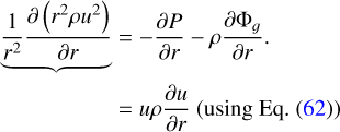
Last, we wanted to verify the order of our spatial reconstruction in spherical coordinates. We proceeded similar to Balsara et al. (2020), using a simple model of a stationary solar wind introduced by Parker (1965). The model expresses a balance of pressure gradient, central gravitational, and inertial force. The radial component of the stationary continuity equation in spherical coordinates is with the radial velocity, u, $$\frac{1}{r^2}\frac{\partial \left(r^2\rho u\right)}{\partial r}=0$$(61) $$\iff -u\frac{\partial \rho }{\partial r}=\rho \frac{\partial u}{\partial r}+\frac{2\rho u}{r}$$(62) $$\Rightarrow \rho ={\rho }_0\left(\frac{u_0}{u}\right){\left(\frac{r_0}{r}\right)}^2,$$(63)

where the last step was obtained by separating the variables from the integration. The momentum equation using the described equilibrium assumptions is $$\begin{array}{l}\underset{}{\underbrace{\frac{1}{r^2}\frac{\partial \left(r^2\rho u^2\right)}{\partial r}}}=-\frac{\partial P}{\partial r}-\rho \frac{\partial {\text{Φ}}_g}{\partial r}.\hfill \\ =u\rho \frac{\partial u}{\partial r}\text{ (using Eq}.\text{ (62)) }\hfill \end{array}$$(64)

Adopting a polytropic equation of state, P = Kρ^γ with ∂_rP = γρ^γ−1∂_rρ, dividing Eq. (65) by ρ, and radially integrating yields $$\frac{u^2-u_0^2}{2}=-\frac{\gamma }{\gamma -1}\left({\rho }^{\gamma -1}-{\rho }_0^{\gamma -1}\right)+GM\left(\frac{1}{r}-\frac{1}{r_0}\right).$$(65)

Equation (44) can then be used to find a density-independent formulation of the momentum equation. Setting all constants except the polytropic index to unity, in other words ρ₀ = r₀ = 1 , we obtain $u_0=c_s=\sqrt{\gamma }$ and arrive at $$\frac{u^2}{2}+\frac{\gamma }{\gamma -1}{u}^{1-\gamma }{r}^{2-2\gamma }-\frac{GM}{r}-\frac{\gamma }{\gamma -1}-\frac{\gamma }{2}+\frac{3}{2}=0.$$(66)

Together with Eq. (63) and the polytropic equation of state, this closes the system.

We solved the continuity equation as well as the momentum equation in spherical coordinates and the radial direction only, using the BDF-2 scheme as well as our slope-limited κ scheme with κ = −1 (LUD). Similar to Balsara et al. (2020), we chose the domain r ∊ [2, 3.5] and used a numerical solution to Eq. (66), which we obtained by using the Pythons SymPy package (Meurer et al. 2017) to calculate ICs for radial velocity and density. We chose γ = 1.4 as well as GM = 1. Equation (66) admits two solutions in the chosen radial domain, one corresponding to a radially decreasing velocity and the other to a radially increasing velocity. Since the former is unphysical, we selected the latter solution where the velocity is supersonic throughout the domain.

We chose the outer boundary as free-flow (inflow and outflow allowed with continuative or zero-gradient approximation) and the inner boundary as constant in time. After some initial numerical relaxation, no transient time evolution is expected. At sufficiently large times, all information about the initial conditions (except those that are engraved in the constant boundary) is lost and the problem is completely defined by the conditions imposed in the constant boundary. We chose a convective CFL number of 0.5 and integrated to the dimensionless time of t_end = 2.5, corresponding to two sound crossing times. The results of the error are shown in Table 2, where we show that the implemented scheme is second order. Here, the error is expressed in terms of the average L₁ loss function over the whole domain. The obtained density and radial velocity alongside their semi-analytic values are shown in Fig. 18.

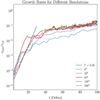Fig. 16 VSI growth rates for different resolutions as a function of the number of orbits covered in comparison to Γ = 0.36 growth. A fit to the 1282 and 2562 runs yields a growth rate of Γ = 0.32 and for the two lower-resolution runs, Γ = 0.4. In all cases, the QUICK and BDF-2 schemes were used.

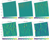Fig. 17 Visualization of the vertical velocity component in the 2562 resolution run for the VSI at different orbital times. The QUICK and BDF-2 schemes were utilized and GMRES was selected as the solver.

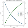Fig. 18 Semi-analytic solution (black lines) and simulated data points (squares) for the solar wind test problem at t = 2.5. BDF-2 was used for temporal integration alongside the LUD scheme for spatial discretization. The simulation was conducted with 200 cells, from which every fourth was used for plotting. The density corresponds to the left axis and the radial velocity to the right axis.

5 Summary and outlook

In this work, we present our novel, globally implicit, time-unsplit and versatile, upwinding-based, finite-volume hydrodynamic solver, MATRICS. We illustrate the numerical spatial discretization schemes used and outline the time integration methodology with the incorporated linear system solvers relying on a matrix-free formulation of the system. The matrix-free approach in combination with the described Newton-Krylov method guarantees easy expandability as well as easier implementation of BCs in the code, which has traditionally been difficult in implicit methods. With tests in different implemented coordinate systems and dimensionalities, we illustrate the operability, accuracy, and correctness of our code and our implementation of the physical mechanisms considered, as well as the inherent strength of the implicit time integration method in not being limited by the Courant number.

In Sect. 4.1, we prove that our code damps sound waves at high Courant numbers but resolves them at lower ones. In Sect. 4.2, we show that our method is able to resolve shocks without producing spurious oscillations close to second order and that, similar to the damping of sound waves, shocks can be damped at high advective Courant numbers. Furthermore, we conducted Sod’s test in spherical coordinates and reproduced results from the literature. With 3D axisymmetric simulations in cylindrical coordinates using resolutions high enough to model the considered physics correctly and including kinematic viscosity, we prove the applicability of our method with moderate computational effort in the example of the TC flow in Sect. 4.3. In Sect. 4.4, we successfully reproduced the isothermal growth rate of the VSI in 3D axisymmetric spherical coordinates at a time step beyond that needed to resolve sound waves. We obtained the expected physical results, which don't rely on resolving sound waves. Finally, in Sect. 4.5, we performed a 1D test in spherical coordinates to prove the second-order accuracy of our method as well as its correctness in spherical coordinates.

The next step in the development process is to improve the parallelization of our solver, where we focus in the short term on OpenMP. After doing so, we will utilize our solver for the modeling of the VSI using long cooling times, which has shown to be problematic using explicit time integration schemes (Manger et al. 2021). We also plan on applying our solver in the context of stellar interiors, starting with modeling of the Goldreich–Schubert–Fricke instability in the radiative zone of stars.

Acknowledgements

The authors thank A.A. Hujeirat for his advisory work during the early development phase of the here presented solver. Part of this work is funded by the DFG via the Heidelberg Cluster of Excellence STRUCTURES in the framework of Germany’s Excellence Strategy (grant EXC-2181/1 – 390900948).

Appendix A Useful identities in axisymmetry

Appendix A.1 Operators in different coordinates

The expression for the gradient used is $$\nabla q=\frac{\partial q}{\partial x}{\mathit{e}}_x+\frac{\partial q}{\partial y}{\mathit{e}}_y\text{\hspace{1em} (Cartesian),}$$(A.1) $$\nabla q=\frac{\partial q}{\partial R}{\mathit{e}}_R+\frac{\partial q}{\partial z}{\mathit{e}}_z\text{\hspace{1em} (Cylindrical),}$$(A.2) $$\nabla q=\frac{\partial q}{\partial r}{\mathit{e}}_r+\frac{1}{r}\frac{\partial q}{\partial \theta }{\mathit{e}}_{\theta }\text{\hspace{1em} (Spherical),}$$(A.3)

the expression for the divergence is $$\nabla \cdot (q\mathit{\upsilon })=\frac{\partial q{\upsilon }_x}{\partial x}+\frac{\partial q{\upsilon }_y}{\partial y}(\text{ Cartesian }),$$(A.4) $$\nabla \cdot (q\mathit{\upsilon })=\frac{1}{R}\frac{\partial \left(q{\upsilon }_R\right)}{\partial R}+\frac{\partial q{\upsilon }_z}{\partial z}(\text{ Cylindrical }),$$(A.5) $$\nabla \cdot (q\mathit{\upsilon })=\frac{1}{r^2}\frac{\partial \left(r^{2}q{\upsilon }_r\right)}{\partial r}+\frac{1}{r\cos \theta }\frac{\partial \left(q{\upsilon }_{\theta }\cos \theta \right)}{\partial \theta }\text{\hspace{0.17em}\hspace{0.17em}\hspace{0.17em}(Spherical)},$$(A.6)

and that for the tensorial divergence is $$\begin{array}{c}\nabla \cdot T=\left(\frac{\partial T_{xx}}{\partial x}+\frac{\partial T_{xz}}{\partial z}\right){\mathit{e}}_x\\ +\left(\frac{\partial T_{zx}}{\partial x}+\frac{\partial T_{zz}}{\partial z}\right){\mathit{e}}_z\\ +\left(\frac{\partial T_{yx}}{\partial x}+\frac{\partial T_{yz}}{\partial z}\right){\mathit{e}}_y,\end{array}$$(A.7)

in Cartesian coordinates, $$\begin{array}{c}\nabla \cdot T=\left(\frac{1}{R}\frac{\partial \left(R\cdot T_{\text{R}R}\right)}{\partial R}+\frac{\partial T_{\text{R}z}}{\partial z}-\frac{T_{\phi \phi }}{R}\right){\mathit{e}}_R\\ +\left(\frac{1}{R}\frac{\partial \left(R\cdot T_{zR}\right)}{\partial R}+\frac{\partial T_{zz}}{\partial z}\right){\mathit{e}}_z\\ +\left(\frac{1}{R}\frac{\partial \left(R\cdot T_{\phi R}\right)}{\partial R}+\frac{\partial T_{\phi z}}{\partial z}+\frac{T_{\text{R}\phi }}{R}\right){\mathit{e}}_{\phi },\end{array}$$(A.8)

in cylindrical coordinates, and $$\begin{array}{l}\nabla \cdot T=\hfill \\ \left(\frac{1}{r^2}\frac{\partial \left(r^2\cdot T_{rr}\right)}{\partial r}+\frac{1}{r\cos \theta }\frac{\partial \left(\cos \theta \cdot T_{r\theta }\right)}{\partial \theta }-\frac{T_{\theta \theta }+T_{\phi \phi }}{r}\right){\mathit{e}}_r\hfill \\ +\left(\frac{1}{r^2}\frac{\partial \left(r^2\cdot T_{\theta r}\right)}{\partial r}+\frac{1}{r\cos \theta }\frac{\partial \left(\cos \theta \cdot T_{\theta \theta }\right)}{\partial \theta }+\frac{T_{r\theta }}{r}\right){\mathit{e}}_{\theta }\hfill \\ +\left(\frac{1}{r^2}\frac{\partial \left(r^2\cdot T_{\phi r}\right)}{\partial r}+\frac{1}{r\cos \theta }\frac{\partial \left(\cos \theta \cdot T_{\phi \theta }\right)}{\partial \theta }+\frac{T_{r\phi }}{r}\right){\mathit{e}}_{\phi }\hfill \\ -\frac{T_{\phi \phi }\cdot \tan \theta }{r}{e}_{\theta }+\frac{T_{\theta \phi }\cdot \tan \theta }{r}{\mathit{e}}_{\phi },\hfill \end{array}$$(A.9)

in spherical coordinates.

Appendix A.2 Components of the viscous stress tensor in different coordinates

The nonzero components of the viscous stress tensor arising from the expression $\underset{{\tau }^{\left(1\right)}}{\underbrace{\mu \left(\mathbf{\nabla }\mathit{\upsilon }+{(\mathbf{\nabla }\mathit{\upsilon })}^T\right)}}$ (see Equation 6) are $${\tau }_{xx}^{(1)}=2\mu \frac{\partial {\upsilon }_x}{\partial x},{\tau }_{yy}^{(1)}=0,{\tau }_{zz}^{(1)}=2\mu \frac{\partial {\upsilon }_z}{\partial z},$$(A.10) $${\tau }_{xy}^{(1)}=\mu \frac{\partial {\upsilon }_y}{\partial x},{\tau }_{yz}^{(1)}=\mu \frac{\partial {\upsilon }_y}{\partial z},{\tau }_{zx}^{(1)}=\mu \left(\frac{\partial {\upsilon }_x}{\partial z}+\frac{\partial {\upsilon }_z}{\partial x}\right)$$(A.11)

in Cartesian Coordinates, $${\tau }_{rr}^{(1)}=2\mu \frac{\partial {\upsilon }_R}{\partial R},{\tau }_{\phi \phi }^{(1)}=2\mu \frac{{\upsilon }_R}{R},{\tau }_{zz}^{(1)}=2\mu \frac{\partial {\upsilon }_z}{\partial z},$$(A.12) $${\tau }_{\text{R}\phi }^{(1)}=\mu R\frac{\partial }{\partial R}\left(\frac{{\upsilon }_{\phi }}{R}\right),{\tau }_{\phi z}^{(1)}=\mu \frac{\partial {\upsilon }_{\phi }}{\partial z},{\tau }_{zr}^{(1)}=\mu \left(\frac{\partial {\upsilon }_R}{\partial z}+\frac{\partial {\upsilon }_z}{\partial R}\right)$$(A.13)

in cylindrical coordinates, and $${\tau }_{rr}^{(1)}=2\mu \frac{\partial {\upsilon }_r}{\partial r},{\tau }_{\theta \theta }^{(1)}=2\mu \left(\frac{1}{r}\frac{\partial {\upsilon }_{\theta }}{\partial \theta }+\frac{{\upsilon }_r}{r}\right),$$(A.14) $${\tau }_{\phi \phi }^{(1)}=2\mu \frac{{\upsilon }_r-{\upsilon }_{\theta }\tan \theta }{r},{\tau }_{r\theta }^{(1)}=\mu \left(r\frac{\partial }{\partial r}\left(\frac{{\upsilon }_{\theta }}{r}\right)+\frac{1}{r}\frac{\partial {\upsilon }_r}{\partial \theta }\right),$$(A.15) $${\tau }_{\theta \phi }^{(1)}=\mu \frac{\cos \theta }{r}\frac{\partial }{\partial \theta }\left(\frac{{\upsilon }_{\phi }}{\cos \theta }\right),{\tau }_{\phi r}^{(1)}=\mu r\frac{\partial }{\partial r}\left(\frac{{\upsilon }_{\phi }}{r}\right)$$(A.16)

in spherical coordinates.

References

- Almgren, A. S., Beckner, V. E., Bell, J. B., et al. 2010, ApJ, 715, 1221 [NASA ADS] [CrossRef] [Google Scholar]
- Andereck, C. D., Liu, S. S., & Swinney, H. L. 1986, J. Fluid Mech., 164, 155 [CrossRef] [Google Scholar]
- Auzinger, W. 1987, Numer. Math., 51, 199 [Google Scholar]
- Balsara, D. S., Garain, S., Florinski, V., & Boscheri, W. 2020, J. Computat. Phys., 404, 109062 [NASA ADS] [CrossRef] [Google Scholar]
- Barrett, R., Berry, M., Chan, T. F., et al. 1994, Templates for the Solution of Linear Systems: Building Blocks for Iterative Methods (Society for Industrial and Applied Mathematics) [CrossRef] [Google Scholar]
- Bastian, P., Müller, E. H., Müthing, S., & Piatkowski, M. 2019, J. Computat. Phys., 394, 417 [NASA ADS] [CrossRef] [Google Scholar]
- Benítez-Llambay, P., & Masset, F. S. 2016, ApJS, 223, 11 [Google Scholar]
- Bird, R. B., Stewart, W. E., & Lightfoot, E. N. 2006, Transport Phenomena (Chichester, England: John Wiley & Sons) [Google Scholar]
- Choquet, R. 1995, A Matrix-Free Preconditioner Applied to CFD, Research Report RR-2605, INRIA [Google Scholar]
- Dorfi, E. A. 1997, in Computational Methods for Astrophysical Fluid Flow (Springer-Verlag), 263 [Google Scholar]
- Esser, A., & Grossmann, S. 1996, Phys. Fluids, 8, 1814 [NASA ADS] [CrossRef] [Google Scholar]
- Ferziger, J. H., & Peric´, M. 2002, Computational Methods for Fluid Dynamics (Springer Berlin Heidelberg) [CrossRef] [Google Scholar]
- Fraysse, F., & Saurel, R. 2019, J. Computat. Phys., 399, 108942 [NASA ADS] [CrossRef] [Google Scholar]
- Guennebaud, G., Jacob, B., Avery, P., et al. 2010, Eigen v3, http://eigen.tuxfamily.org [Google Scholar]
- Hackbusch, W. 1985, Multi-Grid Methods and Applications (Springer Berlin Heidelberg) [CrossRef] [Google Scholar]
- Hai, 1993, Solving Ordinary Differential Equations I (Springer Berlin Heidelberg) [Google Scholar]
- Harlow, F. H., & Welch, J. E. 1965, Phys. Fluids, 8, 2182 [Google Scholar]
- Henson, V. E. 2003, in SPIE Proceedings, eds. C. A. Bouman, & R. L. Stevenson (SPIE) [Google Scholar]
- Hujeirat, A. 2005, Comput. Phys. Commun., 168, 1 [NASA ADS] [CrossRef] [Google Scholar]
- Hujeirat, A., & Rannacher, R. 1998, Int. J. Numer. Methods Fluids, 28, 1 [NASA ADS] [CrossRef] [Google Scholar]
- Hujeirat, A., Camenzind, M., & Keil, B. 2008, New Astron., 13, 436 [NASA ADS] [CrossRef] [Google Scholar]
- Keil, B. W. 2010, Ph.D. Thesis, University ofHeidelberg, Germany [Google Scholar]
- Klahr, H., Baehr, H., & Melon Fuksman, J. D. 2023, ApJ, submitted [arXiv:2305.08165] [Google Scholar]
- Kley, W. 1998, A&A, 338, L37 [Google Scholar]
- Kuo, K. K., & Acharya, R. 2012, Applications of Turbulent and Multiphase Combustion (Wiley) [CrossRef] [Google Scholar]
- Landshoff, R. 1955, A Numerical Method for Treating Fluid Flow in the Presence of Shocks Tech. Rep., LA-1930 [CrossRef] [Google Scholar]
- Leidi, G., Birke, C., Andrassy, R., et al. 2022, A&A, 668, A143 [NASA ADS] [CrossRef] [EDP Sciences] [Google Scholar]
- Leonard, B. 1979, Comput. Methods Appl. Mech. Eng., 19, 59 [NASA ADS] [CrossRef] [Google Scholar]
- Manger, N., & Klahr, H. 2018, MNRAS, 480, 2125 [NASA ADS] [CrossRef] [Google Scholar]
- Manger, N., Klahr, H., Kley, W., & Flock, M. 2020, MNRAS, 499, 1841 [NASA ADS] [CrossRef] [Google Scholar]
- Manger, N., Pfeil, T., & Klahr, H. 2021, MNRAS, 508, 5402 [NASA ADS] [CrossRef] [Google Scholar]
- Meurer, A., Smith, C. P., Paprocki, M., et al. 2017, PeerJ Comput. Sci., 3, e103 [CrossRef] [Google Scholar]
- Mignone, A., Bodo, G., Massaglia, S., et al. 2007, ApJS, 170, 228 [Google Scholar]
- Nelson, R. P., Gressel, O., & Umurhan, O. M. 2013, MNRAS, 435, 2610 [Google Scholar]
- Nowak, U., & Weimann, L. 1992, A Family of Newton Codes for Systems of Highly Nonlinear Equations, Tech. Rep. TR-91-10, ZIB, Berlin [Google Scholar]
- Omang, M., Børve, S., & Trulsen, J. 2006, J. Chem. Phys., 213, 391 [Google Scholar]
- Parker, E. 1965, Space Sci. Rev., 4, 666 [NASA ADS] [CrossRef] [Google Scholar]
- Pearson, J. W., & Pestana, J. 2020, GAMM-Mitteilungen, 43, e202000015 [CrossRef] [Google Scholar]
- Price, H. S., Varga, R. S., & Warren, J. E. 1966, J. Math. Phys., 45, 301 [CrossRef] [Google Scholar]
- Recktenwald, A., Lücke, M., & Müller, H. W. 1993, Phys. Rev. E, 48, 4444 [NASA ADS] [CrossRef] [Google Scholar]
- Saad, Y. 2003, Iterative Methods for Sparse Linear Systems (Society for Industrial and Applied Mathematics) [Google Scholar]
- Saad, Y., & Schultz, M. H. 1986, SIAM J. Sci. Stat. Comput., 7, 856 [CrossRef] [Google Scholar]
- Schrimpf, M., Esteban, J., Warmeling, H., et al. 2021, AIChE J., 67, e17228 [NASA ADS] [CrossRef] [Google Scholar]
- Shadab, M. A., Balsara, D., Shyy, W., & Xu, K. 2019, Comput. Fluids, 190, 398 [CrossRef] [Google Scholar]
- Snyder, H. A. 1968, Phys. Fluids, 11, 1599 [NASA ADS] [CrossRef] [Google Scholar]
- Sod, G. A. 1978, J. Chem. Phys., 27, 1 [NASA ADS] [Google Scholar]
- Springel, V. 2010, Proc. Int. Astron. Union, 6, 203 [NASA ADS] [CrossRef] [Google Scholar]
- Stone, J. M., Mihalas, D., & Norman, M. L. 1992, ApJS, 80, 819 [CrossRef] [Google Scholar]
- Stone, J. M., Gardiner, T. A., Teuben, P., Hawley, J. F., & Simon, J. B. 2008, ApJS, 178, 137 [NASA ADS] [CrossRef] [Google Scholar]
- Taylor, G. I. 1923, Philos. Trans. Roy. Soc. Lond. Ser. A, 223, 289 [NASA ADS] [CrossRef] [Google Scholar]
- Toro, E. F. 2009, Riemann Solvers and Numerical Methods for Fluid Dynamics (Springer Berlin Heidelberg) [Google Scholar]
- Urpin, V., & Brandenburg, A. 1998, MNRAS, 294, 399 [Google Scholar]
- van der Vorst., H. A. 2003, in Iterative Krylov Methods for Large Linear Systems, Cambridge Monographs on Applied and Computational Mathematics (Cambridge University Press) [Google Scholar]
- van Leer, B. 1979, J. Chem. Phys., 32, 101 [NASA ADS] [Google Scholar]
- Viallet, M., Baraffe, I., & Walder, R. 2011, A&A, 531, A86 [NASA ADS] [CrossRef] [EDP Sciences] [Google Scholar]
- VonNeumann, J., & Richtmyer, R. D. 1950, J. Appl. Phys., 21, 232 [NASA ADS] [CrossRef] [Google Scholar]
- Wang, S., & Johnsen, E. 2017, arXiv e-prints [arXiv: 1701.04834] [Google Scholar]
- Zhang, D., Jiang, C., Liang, D., & Cheng, L. 2015, J. Computat. Phys., 302, 114 [NASA ADS] [CrossRef] [Google Scholar]
All Tables
Comparison of average L1 errors with respect to density for the slope-limited version of QUICK and LUD, respectively, for different spatial resolutions.