| Issue |
A&A
Volume 695, March 2025
|
|
|---|---|---|
| Article Number | A170 | |
| Number of page(s) | 21 | |
| Section | Numerical methods and codes | |
| DOI | https://doi.org/10.1051/0004-6361/202452770 | |
| Published online | 19 March 2025 | |
PySCo: A fast particle-mesh N-body code for modified gravity simulations in Python
1
Université Paris-Saclay, Université Paris Cité, CEA, CNRS, AIM,
91191,
Gif-sur-Yvette, France
2
Institute of Space Sciences (ICE, CSIC), Campus UAB,
Carrer de Can Magrans, s/n,
08193
Barcelona, Spain
3
Laboratoire Univers et Théorie, Observatoire de Paris, Université PSL, Université Paris Cité, CNRS,
92190
Meudon, France
★ Corresponding author; This email address is being protected from spambots. You need JavaScript enabled to view it.
Received:
27
October
2024
Accepted:
18
February
2025
Abstract
We present PySCo, a fast and user-friendly Python library designed to run cosmological N-body simulations across various cosmological models, such as ΛCDM (Λ with cold dark matter) and w0waCDM, and alternative theories of gravity, including f (R), MOND (modified newtonian dynamics) and time-dependent gravitational constant parameterisations. PySCo employs particle-mesh solvers, using multigrid or fast Fourier transform (FFT) methods in their different variations. Additionally, PySCo can be easily integrated as an external library, providing utilities for particle and mesh computations. The library offers key features, including an initial condition generator based on up to third-order Lagrangian perturbation theory (LPT), power spectrum estimation, and computes the background and growth of density perturbations. In this paper, we detail PySCo’s architecture and algorithms and conduct extensive comparisons with other codes and numerical methods. Our analysis shows that, with sufficient small-scale resolution, the power spectrum at redshift z = 0 remains independent of the initial redshift at the 0.1% level for zini ≥ 125, 30, and 10 when using first, second, and third-order LPT, respectively. Moreover, we demonstrate that acceleration (or force) calculations should employ a configuration-space finite-difference stencil for central derivatives with at least five points, as three-point derivatives result in significant power suppression at small scales. Although the seven-point Laplacian method used in multigrid also leads to power suppression on small scales, this effect can largely be mitigated when computing ratios. In terms of performance, PySCo only requires approximately one CPU hour to complete a Newtonian simulation with 5123 particles (and an equal number of cells) on a laptop. Due to its speed and ease of use, PySCo is ideal for rapidly generating vast ensemble of simulations and exploring parameter spaces, allowing variations in gravity theories, dark energy models, and numerical approaches. This versatility makes PySCo a valuable tool for producing emulators, covariance matrices, or training datasets for machine learning.
Key words: methods: numerical / cosmology: miscellaneous / large-scale structure of Universe
© The Authors 2025
 Open Access article, published by EDP Sciences, under the terms of the Creative Commons Attribution License (https://creativecommons.org/licenses/by/4.0), which permits unrestricted use, distribution, and reproduction in any medium, provided the original work is properly cited.
This article is published in open access under the Subscribe to Open model. This email address is being protected from spambots. You need JavaScript enabled to view it. to support open access publication.
1 Introduction
On the largest scales, the ΛCDM (Λ with cold dark matter) model provides a robust description of our Universe, where dark energy is represented as a cosmological constant (Λ) and dark matter as non-relativistic cold dark matter (Planck Collaboration VI 2020; Alam et al. 2021; Riess et al. 2022). The ΛCDM model also assumes General Relativity (GR), which offers an accurate representation of the Universe by incorporating small perturbations on a Friedman–Lemaître–Robertson–Walker (FLRW) background (Green & Wald 2014). The formation of the large-scale structure is driven by these small perturbations, which grow over time through gravitational interactions, giving rise to the cosmic web observed today (Peebles 1980).
While linear theory can analytically describe the growth of perturbations on large scales above ~100 Mpc (Yoo et al. 2009; Bonvin & Durrer 2011; Challinor & Lewis 2011), the non-linear nature of structure formation on smaller scales necessitates more advanced approaches. Higher-order perturbation theory, both in its Eulerian (Peebles 1980; Bernardeau et al. 2002) and Lagrangian (Zel’dovich 1970; Buchert & Ehlers 1993) formulations, allows for a more accurate understanding down to scales of ~20 Mpc. Below this scale, structure formation becomes highly non-linear, and the evolution of gravitationally interacting particles can only be accurately modeled through N-body simulations (Efstathiou et al. 1985).
Over time, numerous cosmological N -body codes have been developed (Couchman 1991; Kravtsov et al. 1997; Knebe et al. 2001; Teyssier 2002; Ishiyama et al. 2009; Potter et al. 2017; Springel et al. 2021; Garrison et al. 2021), with recent simulations including trillions of particles (Ishiyama et al. 2021; Euclid Collaboration: Castander et al. 2025). While significant effort has been invested in developing efficient Newtonian simulations for cosmology (see Angulo & Hahn 2022 for a review), many N -body codes for alternative gravity theories are derived from Newtonian codes. For instance, ECOSMOG (Li et al. 2012), ISIS (Llinares et al. 2014), RayMOND (Candlish et al. 2015), and Phantom of RAMSES (Lüghausen et al. 2015) are all based on the RAMSES code (Teyssier 2002). The former two implement the f (R) model (Hu & Sawicki 2007) and the nDGP model (Dvali et al. 2000), while the latter two implement MOND (modified newtonian dynamics, Milgrom 1983). Although it is possible to integrate modified gravity theories into TreePM codes like Gadget (Springel et al. 2021), as demonstrated by MG-Gadget (Puchwein et al. 2013), RAMSES has emerged as the preferred code for such implementations. This is due to the fact that alternative theories of gravity generally introduce additional fields governed by non-linear partial differential equations, which cannot be efficiently solved using standard tree-based methods. As a result, RAMSES, a particle-mesh (PM) code with adaptive-mesh refinement (AMR) and a multigrid solver, becomes an ideal choice for implementing these features. However, PM-AMR, TreePM, or Fast Multipole Method (FMM) codes typically require significant computational resources, even when highly optimised. This challenge is exacerbated in simulations of alternative gravity theories; for instance, Euclid Collaboration: Adamek et al. (2025) showed that f (R) or nDGP simulations can run up to ten times slower than their Newtonian counterparts.
To address these computational demands, researchers have explored PM codes (Knebe et al. 2001; Merz et al. 2005; Feng et al. 2016; Adamek et al. 2016; Klypin & Prada 2018) to reduce the cost at the expense of small-scale accuracy. These faster, albeit less precise, simulations are suitable for specific applications, such as producing large numbers of realisations for covariance matrix estimation or calculating the ratio (or boost) of specific statistical quantities relative to a reference case exploring large parameter spaces. Furthermore, exact PM codes can accurately reproduce structure formation at small scales given a higher resolution of the uniform mesh. Consequently, such codes have been ideal for developing solvers for modified gravity theories (see Llinares 2018 for a review), and have been used to study their impact relative to Newtonian simulations (Valogiannis & Bean 2017; Winther et al. 2017; Hassani & Lombriser 2020; Ruan et al. 2022; Hernández-Aguayo et al. 2022).
Given the need for speed, most N-body simulations have traditionally been written in compiled languages such as Fortran, C, or C++. In contrast, Python has become the most popular programming language in data science, owing to its straightforward syntax, rapid development speed, and extensive community- driven libraries, especially in astronomy. This popularity has created a gap between simulators and the broader scientific field. Despite its advantages, Python is often viewed as a slow language when used natively. To address this, significant effort has gone into developing efficient Python libraries, either as wrappers for C-based codes (such as NumPy, Harris et al. 2020) or through compiling Python code to machine language, as seen in Numba (Lam et al. 2015) and Cython (Behnel et al. 2011). Recently, the latter approach was used to develop the P3M code CONCEPT (Dakin et al. 2022), demonstrating the viability of Python for high-performance applications.
In this paper, we present PySCo1 (Python Simulations for Cosmology), a cosmological PM N -body code written in Python and utilising the Numba library for increased performance and multithreading. The paper is organised as follows: Section 2 introduces the different models implemented in PySCo, including the modified gravity theories f (R) from Hu & Sawicki (2007), MOND (Milgrom 1983), parameterised gravity (Amendola et al. 2008), and dynamic dark energy (Chevallier & Polarski 2001; Linder 2003). Section 3 details the structure and algorithms implemented in the code, covering initial condition generation and various N-body solvers. In Section 4, we validate PySCo against other codes and analyse the impact of different numerical methods on the matter power spectrum. Finally, we conclude in Section 5.
2 Theory
2.1 Newtonian gravity
Let us consider only scalar perturbations on FLRW metric, in the Newtonian gauge (Ma & Bertschinger 1995)
![Mathematical equation: ${\rm{d}}{s^2} = {a^2}(\eta )\left[ { - (1 + 2\psi ){\rm{d}}{\eta ^2} + (1 - 2\phi ){\rm{d}}{x^2}} \right],$](/articles/aa/full_html/2025/03/aa52770-24/aa52770-24-eq1.png) (1)
(1)
with a the scale factor, η the conformal time and ψ and ф the Bardeen potentials (Bardeen 1980). In GR, we have ψ = ф, and the Einstein equation gives
 (2)
(2)
with ℋ = aH the conformal Hubble parameter, ф′ the time derivative of the potential and ρ the Universe’s components density. It is common to apply the Newtonian and quasi-static (neglecting time derivatives) approximations, which involve neglecting the second term on the left-hand side of Eq. (2), as it is only significant at horizon scales. In the context of Newtonian cosmology, the Einstein equation takes the same form as the classical Poisson equation, with an additional dependence on the scale factor
 (3)
(3)
with ρm the matter density. There are, however, cosmological General Relativity (GR) simulations (Adamek et al. 2016; Barrera-Hinojosa & Li 2020) that solve the full Einstein equations in the weak-field limit, taking into account gauge issues (Fidler et al. 2015, 2016). Additionally, there are methods to interpret Newtonian simulations within a relativistic framework (Chisari & Zaldarriaga 2011; Adamek & Fidler 2019). In this work, however, we focus on smaller scales where relativistic effects are negligible, and the Newtonian approximation remains well justified.
2.2 Dynamical dark energy
The w0waCDM model provides a useful phenomenological extension of the standard ΛCDM framework by offering a dynamic, time-dependent description of dark energy. In this model, the cosmological constant is replaced by a variable dark energy component, which affects the formation of cosmic structures by modifying the universe’s expansion history. For a flat geometry (Ωk = 0), the Hubble parameter H(z) is given by
 (4)
(4)
where a subscript zero indicates a present-day evaluation, and Ωm, Ωr, and Ωλ represent the density fractions of matter, radiation, and dark energy, respectively. In this model, the dark-energy density evolves with redshift, following the relation
![Mathematical equation: ${{\rm{\Omega }}_{\rm{\Lambda }}}() = {{\rm{\Omega }}_{{\rm{\Lambda }},0}}\exp \left\{ {\mathop \smallint \limits_0^ {{3\left[ {1 + w\left( {'} \right)} \right]{\rm{d}}'} \over {1 + '}}} \right\}.$](/articles/aa/full_html/2025/03/aa52770-24/aa52770-24-eq5.png) (5)
(5)
Using the widely adopted CPL parametrisation (Chevallier & Polarski 2001; Linder 2003), the dark-energy equation of state is expressed as
 (6)
(6)
This simple modification does not alter the Einstein field equations nor the equations of motion, and it recovers the standard ΛCDM model when w0 = −1 and wa = 0.
2.3 MOND gravity
The Modified Newtonian Dynamics (MOND) theory, introduced by Milgrom (1983), was proposed as a potential solution to the dark matter problem by suggesting a deviation from Newtonian gravity in a Universe where the matter content is entirely in the form of baryons (for a detailed review, see Famaey & McGaugh 2012). In MOND, Newton’s second law is modified as follows
 (7)
(7)
where g and gN represent the MOND and Newtonian accelerations, respectively, and g0 is a characteristic acceleration scale, approximately g0 ≈ cH0/[2π] ≈ 10−10m.s−2. The function µ(x) is an interpolating function that governs the transition between the Newtonian regime (where gravitational force scales as r−2) and the MOND regime (where the force scales as r−1), with r being the separation between masses. The interpolating function has the following limits
 (8)
(8)
Similarly, the inverse interpolating function ν(y) can be defined as
 (9)
(9)
where ν(y) follows the limits
 (10)
(10)
In the MOND framework, the classical Poisson equation is modified as follows (Bekenstein & Milgrom 1984)
![Mathematical equation: $\nabla \left[ {\mu \left( {{{\left| {\nabla \phi } \right|} \over {{g_0}}}} \right)\nabla \phi } \right] = 4\pi G\delta \rho ,$](/articles/aa/full_html/2025/03/aa52770-24/aa52770-24-eq11.png) (11)
(11)
a formulation known as AQUAL, derived from a quadratic Lagrangian. In this paper, however, we consider the QUMOND (quasi-linear MOND, Milgrom 2010) formulation, where the non-linearity in the Poisson equation is re-expressed in terms of an additional effective dark matter fluid in the source term. The modified Poisson equations are
 (12)
(12)
![Mathematical equation: ${\nabla ^2}\phi = \nabla \left[ {v\left( {\left| {\nabla {\phi ^{\rm{N}}}} \right|/{_0}} \right)\nabla {\phi ^{\rm{N}}}} \right],$](/articles/aa/full_html/2025/03/aa52770-24/aa52770-24-eq13.png) (13)
(13)
where фN and ф are the Newtonian and MOND potentials, respectively. This system of equations is more convenient to solve, as it involves only two linear Poisson equations. Moreover, numerical simulations have demonstrated that the AQUAL and QUMOND formulations yield very similar results (Candlish et al. 2015).
The missing component in the MOND framework is the specific form of the ν(y) function. Several families of interpolating functions have been proposed, each with different characteristics
-
Simple function:
 (14)
(14)which corresponds to the simple function proposed by Famaey & Binney (2005), equivalent to µ(x) = x/(1 + x).
-
The n-family:
![Mathematical equation: $v(y) = {\left[ {{1 \over 2} + {{\sqrt {1 + 4/{y^n}} } \over 2}} \right]^{1/n}},$](/articles/aa/full_html/2025/03/aa52770-24/aa52770-24-eq15.png) (15)
(15)a commonly used parametrisation for the interpolating function (Milgrom & Sanders 2008). The case n = 2 is particularly well studied and is known as the standard interpolating function (Begeman et al. 1991). Additionally, Milgrom & Sanders (2008) introduced other functional forms
The β-family:
 (16)
(16)The γ-family:
 (17)
(17)-
The δ-family:
 (18)
(18)which is a subset of the γ-family. While we focus on non- relativistic formulations of MOND for simplicity, it is important to acknowledge that various relativistic frameworks have been developed (Bekenstein 2006; Milgrom 2009; Skordis & Złośnik 2021), along with a recent generalisation of QUMOND (Milgrom 2023). These topics, however, are beyond the scope of this paper.
2.4 Parametrised gravity
A straightforward and effective phenomenological approach to modifying the theory of gravity is through the µ − σ parametrisation of the Einstein equations (Amendola et al. 2008). This is particularly useful when considering unequal Bardeen potentials ф ≠ ψ. Under the Newtonian and quasi-static approximations, the Einstein equations can be expressed as
 (19)
(19)
 (20)
(20)
where µ(a) represents the time-dependent ‘effective gravitational coupling’, which can be interpreted as a modification of the gravitational constant, and Σ(a) is the ‘light deflection parameter’. Since our focus is on the evolution of dark-matter particles, we only need to implement Eq. (19), which involves µ(a). In practice, the gravitational coupling µ(a) could be a function of both time and scale in Fourier space, µ(a, k), as in the ‘effective-field theory of dark energy’ (Frusciante & Perenon 2020). However, for simplicity, we prefer methods that can be solved numerically in both Fourier and configuration space. The inclusion of scale-dependent corrections will be considered in future work.
For the functional form of µ(a), we use the parametrisation from Simpson et al. (2013); Planck Collaboration XIV (2016); Planck Collaboration VI (2020); Abbott et al. (2019), which allows for deviations from GR during a dark-energy dominated era
 (21)
(21)
where µ0 is the only free parameter, representing the gravitational coupling today.
2.5 f(R) gravity
In f (R) gravity, the Lagrangian extends the Einstein-Hilbert action (GR) by including an arbitrary function of the Ricci scalar curvature R. The total action is given as (Buchdahl 1970; Sotiriou & Faraoni 2010)
![Mathematical equation: $S = \mathop \smallint \nolimits^ {{\rm{d}}^4}x\sqrt { - } \left[ {{{R + f(R)} \over {16\pi G}} + {{\cal L}_m}} \right],$](/articles/aa/full_html/2025/03/aa52770-24/aa52770-24-eq22.png) (22)
(22)
where ℒm represents the matter Lagrangian, G is the gravitational constant, g is the determinant of the metric, and f (R) is the additional function of the curvature, which reduces to −2Λ in the standard ΛCDM model. A commonly used parametrisation of f (R) gravity is provided by Hu & Sawicki (2007), with the following functional form
 (23)
(23)
 (24)
(24)
where n, c1 and c2 are the model parameters, and m represents the curvature scale, given by  , where
  is the current mean matter density. This model incorporates a Chameleon screening mechanism (Khoury & Weltman 2004; Burrage & Sakstein 2018) to suppress the fifth force caused by the scalar field fR (also known as the ‘scalaron’). The scalaron is given by
 (25)
(25)
which allows the theory to recover GR in high-density environments, ensuring consistency with Solar System tests. Observational evidence for dark energy as a cosmological constant imposes the constraint
 (26)
(26)
and we can also express
![Mathematical equation: ${{{c_1}} \over {c_2^2}} = - {3 \over n}{\left[ {1 + 4{{{{\rm{\Omega }}_{{\rm{\Lambda }},0}}} \over {{{\rm{\Omega }}_{m,0}}}}} \right]^{n + 1}}{f_{R0}},$](/articles/aa/full_html/2025/03/aa52770-24/aa52770-24-eq29.png) (27)
(27)
where fR0 is the present-day value of the scalaron, with current observational constraints from galaxy clusters indicating log10 fR0 < −5.32 (Vogt et al. 2025). In this framework, the Poisson equation is modified compared to its Newtonian counterpart. There is an additional term that depends on the scalaron field
 (28)
(28)
 (29)
(29)
where the difference in curvature is given by
![Mathematical equation: $\delta R = R - \bar R = \bar R\left[ {{{\left( {{{{{\bar f}_R}} \over {{f_R}}}} \right)}^{1/(n + 1)}} - 1} \right].$](/articles/aa/full_html/2025/03/aa52770-24/aa52770-24-eq32.png) (30)
(30)
Here,  represents the background curvature, expressed as
 (31)
(31)
and  is the background value of fR
 (32)
(32)
The primary observational distinction between f (R) gravity and GR lies in the enhanced clustering on small scales, with the amplitude and shape of these deviations being dependent on fR0, despite the two models sharing the same overall expansion history.
3 Methods
This section reviews the numerical methods used in PySCo, from generating initial conditions to evolving dark-matter particles in N-body simulations across various theories of gravity.
PySCo is entirely written in Python and uses the open-source library Numba (Lam et al. 2015), which compiles Python code into machine code using the LLVM compiler. This setup combines Python’s high development speed and rich ecosystem with the performance of C/Fortran. To optimise performance, PySCo relies on writing native Python code with ‘for’ loops, similar to how it would be done in C or Fortran.
Numba integrates seamlessly with NumPy (Harris et al. 2020), a widely used package for numerical operations in Python. Parallelisation in PySCo is simplified: by replacing ‘range’ with ‘prange’ in loops, the code takes advantage of multi-core processing. Numba functions are typically compiled just-in-time (JIT), meaning they are compiled the first time the function is called. Numba infers input and output types dynamically, supporting function overloading for different types.
In PySCo, however, most functions are compiled ahead-of- time (AOT), meaning they are compiled as soon as the code is executed or imported. This is because the simulation uses 32-bit floating point precision for all fields, allowing for AOT compilation. Since the simulation operates on a uniform grid, unlike AMR simulations, there is no need for fine-grained grids. Therefore, using 32-bit precision is sufficient and does not result in any loss of accuracy. Additionally, 32-bit floats improve performance by enabling SIMD (Single Instruction, Multiple Data) instructions, which the compiler implicitly optimises for.
3.1 Units and conventions
We adopt the same strategy as RAMSES and use supercomoving units (Martel & Shapiro 1998), where the Poisson equation takes the same form as in classical Newtonian dynamics but includes a multiplicative scale factor
 (33)
(33)
where a tilde denotes a quantity in supercomoving units, a is the scale factor, ф the gravitational potential, and ρ the matter density. We also define conversion units from comoving coordinates and super-conformal time to physical SI units
 (34)
(34)
 (35)
(35)
where  and
and  represent the particle position, time and velocity, gravitational potential and speed of light in simulation units. The conversion factors are defined as follows
 (36)
(36)
 (37)
(37)
 (38)
(38)
as the length, time and density conversion units to km2, seconds and kg/m3 respectively, where Lbox is the box length in comoving coordinates and H0 is the Hubble parameter today (in seconds). The particle mass is given by
 (39)
(39)
where Npart is the total number of particles in the simulation.
3.2 Data structure
In this section, we discuss how PySCo handles the storage of particles and meshes using C-contiguous NumPy arrays. This approach was chosen for its simplicity and readability, allowing functions in PySCo to be easily reused in different contexts.
For particles, the position and velocity arrays are stored with the shape [Npart, 3], where the elements for each particle are contiguous in memory. This format is more efficient than using a shape of [3, Npart], particularly for mass assignment, where operations are performed particle by particle. To further enhance performance, particles are ordered using Morton indices (also known as z-curve indices) rather than linear or random ordering. Morton ordering improves cache usage and, thus, increases performance. This ordering is applied every Nreorder steps, as defined by the user, to maintain good data locality and avoid performance losses (see also Appendix E). We did not consider space-filling curves with better data locality properties (such as the Hilbert curve), because the associated encoding and decoding algorithms are much more computationally expensive, and Morton curves already provide excellent data locality. While more complex data structures are available (such as linked lists, fully-threaded trees, octrees or kdtrees), preliminary tests showed that using Morton-ordered NumPy arrays strikes a good balance between simplicity and performance, without the overhead of creating complex structures.
For scalar fields on the grid, arrays are stored with a shape ![Mathematical equation: $\left[ {N_{{\rm{cells}}}^{1/3},N_{{\rm{cells}}}^{1/3},N_{{\rm{cells}}}^{1/3}} \right]$](/articles/aa/full_html/2025/03/aa52770-24/aa52770-24-eq46.png) using linear indexing. Although linear indexing does not offer optimal data locality, it is lightweight and does not require additional arrays to store indices. Moreover, it works well with predictable (optimizable) memory-access patterns, such as those used in stencil operators. For vector fields, such as acceleration, the arrays have a shape
using linear indexing. Although linear indexing does not offer optimal data locality, it is lightweight and does not require additional arrays to store indices. Moreover, it works well with predictable (optimizable) memory-access patterns, such as those used in stencil operators. For vector fields, such as acceleration, the arrays have a shape ![Mathematical equation: $\left[ {N_{{\rm{cells}}}^{1/3},N_{{\rm{cells}}}^{1/3},N_{{\rm{cells}}}^{1/3},3} \right]$](/articles/aa/full_html/2025/03/aa52770-24/aa52770-24-eq47.png) , similar to the format used for particle arrays, to maintain consistency and performance.
, similar to the format used for particle arrays, to maintain consistency and performance.
3.3 Initial conditions
In this section, we describe how PySCo handles the generation of initial conditions for simulations, although it can also read from pre-existing snapshots in other formats. PySCo can load data directly from RAMSES/pFoF format used in the Ray- Gal simulations (Breton et al. 2019; Rasera et al. 2022) or from Gadget format using the Pylians library (Villaescusa-Navarro 2018>). PySCo computes the time evolution of the scale factor, growth factors, and Hubble parameters, with the Astropy library (Astropy Collaboration 2022) and internal routines (see Appendix A).
To generate the initial conditions, the code requires a linear power spectrum P(k, z = 0), which is rescaled by the growth factor at the initial redshift zini. Additionally, PySCo generates a realisation of Gaussian white noise W, which is used to apply initial displacements to particles.
Some methods generate Gaussian white noise in configuration space, which is particularly useful for zoom simulations (Pen 1997; Sirko 2005; Bertschinger 2001; Prunet et al. 2008; Hahn & Abel 2013). However, in PySCo, the white noise is computed as
 (40)
(40)
with A(k) an amplitude drawn from a Rayleigh distribution given by ![Mathematical equation: ${{\cal R}_{{\rm{dist}}}} = \sqrt { - \ln {\cal U}]0,1]} $](/articles/aa/full_html/2025/03/aa52770-24/aa52770-24-eq49.png) with U]0,1] a uniform random sampling between 0 and 1, and θ(k) = U]0,1]. We also fix
with U]0,1] a uniform random sampling between 0 and 1, and θ(k) = U]0,1]. We also fix  where a bar denotes a complex conjugate, to ensure that the configuration-space field is real valued. In our case, since we consider a regular grid with periodic boundary conditions, we can generate the white noise directly in Fourier space. An initial realisation of a density field is computed using
 (41)
(41)
with k = |k|. This ensures that we recover the Gaussian properties
 (42)
(42)
 (43)
(43)
where δD is a Dirac delta and δini(0) = 0. We have also implemented the option to use ‘paired and fixed’ initial conditions (Angulo & Pontzen 2016). This method greatly reduces cosmic variance by running paired simulations with opposite phases, at the cost of introducing some non-Gaussian features. The concept here is that instead of averaging the product of modes to match the power spectrum, the individual modes are set directly to  . In practice, the density field is used to compute the initial particle displacement from a homogeneous distribution, rather than directly sampling δini . We use Lagrangian perturbation theory (LPT), with options for first- order 1LPT (also called ‘Zel’dovich approximation’, Zel’dovich 1970), second-order 2LPT (Scoccimarro 1998; Crocce et al. 2006), or third-order 3LPT (Catelan 1995; Rampf & Buchert 2012). The displacement field at the initial redshift zini up to third order is expressed as
 (44)
(44)
with D+ ≡ D+(zini)(1) is the linear (first order) growth factor at the initial redshift and Ψ(n) are the different orders of the displacement field at z = 0, which can be written as (Michaux et al. 2021)
 (45)
(45)
 (46)
(46)
 (47)
(47)
 (48)
(48)
 (49)
(49)
 (50)
(50)
![Mathematical equation: ${{\phi ^{(2)}} = {1 \over 2}{\nabla ^{ - 2}}\left[ {\phi _{,ii}^{(1)}\phi _{,jj}^{(1)} - \phi _{,ij}^{(1)}\phi _{,ij}^{(1)}} \right],}$](/articles/aa/full_html/2025/03/aa52770-24/aa52770-24-eq62.png) (51)
(51)
![Mathematical equation: ${{\phi ^{(3a)}} = {\nabla ^{ - 2}}\left[ {\det \phi _{,ij}^{(1)}} \right],}$](/articles/aa/full_html/2025/03/aa52770-24/aa52770-24-eq63.png) (52)
(52)
![Mathematical equation: ${\phi ^{(3b)}} = {1 \over 2}{\nabla ^{ - 2}}\left[ {\phi _{,ii}^{(2)}\phi _{,jj}^{(1)} - \phi _{,ij}^{(2)}\phi _{ij}^{(1)}} \right],$](/articles/aa/full_html/2025/03/aa52770-24/aa52770-24-eq64.png) (53)
(53)
![Mathematical equation: ${A^{(3c)}} = {\nabla ^{ - 2}}\left[ {\nabla \phi _{,i}^{(2)} \times \nabla \phi _{,i}^{(1)}} \right],$](/articles/aa/full_html/2025/03/aa52770-24/aa52770-24-eq65.png) (54)
(54)
and
 (55)
(55)
 (56)
(56)
 (57)
(57)
 (58)
(58)
 (59)
(59)
 (60)
(60)
In practice, we compute all derivatives directly in Fourier space, since configuration-space finite-difference gradients would smooth the small scales and thus create inaccuracies in the initial power spectrum. The second- and third-order contributions in the initial conditions can be prone to aliasing effects due to the quadratic and cubic non-linearities involved. To mitigate this, we apply Orszag’s 3/2 rule (Orszag 1971), as suggested in Michaux et al. (2021). The impact of this correction is minimal, by around 0.1% on the power spectrum at small scales, when using 3LPT initial conditions and for a relatively late start with zini ≈ 10). The initial position and velocity are then (up to third order)
 (61)
(61)
 (62)
(62)
 (63)
(63)
 (64)
(64)
with H the Hubble parameter at zini, fn the growth rate contribution to the n-th order, and xuniform the position of cell centres (or cell edges, see also Appendix B.2) when Npart = Ncells. We internally compute the growth factor and growth rate contributions as described in Appendix A.
3.4 Integrator
In our simulations, we employ the second-order symplectic Leapfrog scheme, often referred to as Kick-Drift-Kick, to integrate the equations of motion for the particles. The steps in the scheme are as follows
 (65)
(65)
where the subscript i indicates the integration step, while x, v and a are the particle positions, velocities and accelerations respectively. There are several ways to set the time step ∆t. Some authors use linear or logarithmic spacing, depending on the user input. In our case, we followed a similar strategy as RAMSES (Teyssier 2002) and use several time stepping criteria. The first criterion is based on a cosmological time step that guarantees the scale factor does not change by more than a specified amount (by default 2%, see also Appendix B.1), which is particularly effective at high redshift. The second criterion is based on the minimum free-fall time given by
 (66)
(66)
with h the cell size. We select the smallest value between this criterion and the cosmological time step. Additionally, we implemented a third criterion based on particle velocities ∆tvel = h/max(|vi|), though we found this value often exceeds ∆tff in practice. This approach ensures that the time step dynamically adapts to the structuration of dark matter in the simulation. To further refine the time step, we multiply it by a user-defined Courant-like factor.
An interesting prospect for the future is the use of integrators based on Lagrangian perturbation theory (LPT) that could potentially reduce the number of time steps required while maintaining high accuracy (as suggested by Rampf et al. 2025). However, such methods couple the integration scheme with specific theories of gravity through growth factors. Since these factors may not always be accurately computed (for example, in MOND), we prefer to maintain the generality of the standard leapfrog integration scheme for now. We may explore the implementation of such LPT-based integrators in the future for specific theories of gravitation.
3.5 Iterative solvers
To displace the particles, we first need to compute the force (or acceleration). There are various algorithms available for this purpose, either computing the force directly from a particle distribution, or determining the gravitational potential from which the force can subsequently be derived. When using the gravitational potential approach, the force can be recovered by applying a finite-difference gradient operator g = −∇ϕ. Given that our results are sensitive to the order of the operator used, we have implemented several options for central difference methods, each characterised by specific coefficients. These coefficients are detailed in Table 1. We aim to solve the following problem
 (67)
(67)
Where u is unknown, f is known and L is an operator. For the classical Poisson equation, u ≡ ϕ, f ≡ 4πGρ and L ≡∇2 with the seven-point Laplacian stencil
 (68)
(68)
with the subscripts i, j, k the cell indices and Li,j,k(u) = ui + 1,j,k + ui,j +1, k + ui,j, k +1 + ui−1,j, k + ui,j −1, k + ui,j,k − 1.
Lastly, f is the density (source) term of Eq. (67), which is directly estimated from the position of dark-matter particles. In code units, the sum of the density over the full grid must be
 (69)
(69)
where the density in a given cell is computed using the ‘nearestgrid point’ (NGP), ‘cloud-in-cell’ (CIC) or ‘triangular-shaped cloud’ (TSC) mass-assignment schemes
 (70)
(70)
 (71)
(71)
 (72)
(72)
Here, xi is the normalised separation between a particle and cell positions, scaled by the cell size. In a three-dimensional space, this implies that a dark-matter particle contributes to the density of one, eight, or twenty-seven cells depending on whether the NGP, CIC, or TSC scheme is employed, respectively. For consistency, we use the same (inverse) scheme to interpolate the acceleration from cells to particles.
Stencil operator coefficients for central derivatives.
3.6 The Jacobi and Gauss-Seidel methods
Let us consider ![Mathematical equation: ${\cal L} = \left[ {\matrix{ {{\ell _{11}}} & {{\ell _{12}}} & {{\ell _{13}}} & \ldots & {{\ell _{1n}}} \cr {{\ell _{21}}} & {{\ell _{22}}} & {{\ell _{23}}} & \ldots & {{\ell _{2n}}} \cr \vdots & \vdots & \vdots & \ddots & \vdots \cr {{\ell _{n1}}} & {{\ell _{n2}}} & {{\ell _{n3}}} & \ldots & {{\ell _{nn}}} \cr } } \right],u = \left[ {\matrix{ {{u_1}} \cr {{u_2}} \cr \vdots \cr {{u_n}} \cr } } \right]$](/articles/aa/full_html/2025/03/aa52770-24/aa52770-24-eq97.png) and
and ![Mathematical equation: $f = \left[ {\matrix{ {{f_1}} \cr {{f_2}} \cr \vdots \cr {{f_n}} \cr } } \right]$](/articles/aa/full_html/2025/03/aa52770-24/aa52770-24-eq98.png) The Jacobi method is a naive iterative solver which, for Eq. (67), takes the form
The Jacobi method is a naive iterative solver which, for Eq. (67), takes the form
 (73)
(73)
 (74)
(74)
 (75)
(75)
 (76)
(76)
where the superscripts ‘new’ and ‘old’ refer to the iteration. This means that for one Jacobi sweep, the new value is directly given by that of the previous iteration.
In practice, we use the Gauss-Seidel method instead, which has a better convergence rate and lower memory usage. This method is akin to Jacobi’s but enhances convergence by incorporating the most recently updated values in the computation of the remainder. It follows
 (77)
(77)
 (78)
(78)
 (79)
(79)
 (80)
(80)
which seems impossible to parallelise because each subsequent equation relies on the results of the previous one. However, we implement a strategy known as ‘red-black’ ordering in the Gauss-Seidel method. This technique involves colouring the cells like a chessboard, where each cell is designated as either red or black. When updating the red cells, we only utilise information from the black cells, and vice versa. This approach is equivalent to performing two successive Jacobi sweeps—one for the red cells and another for the black cells. For the Laplacian operator as expressed in Eq. (68), the Jacobi sweep for a given cell can be formulated as follows
 (81)
(81)
In scenarios involving a non-linear operator, finding an exact solution may not be feasible. In such cases, we linearise the operator using the Newton-Raphson method, expressed as
 (82)
(82)
This approach is commonly referred to as the ‘Newton Gauss- Seidel method’, allowing for more effective convergence in nonlinear contexts.
3.7 Multigrid
In practice, both the Jacobi and Gauss-Seidel methods are known for their slow convergence rates, often requiring hundreds to thousands of iterations to reach a solution and typically unable to achieve high accuracy. To overcome these limitations, a popular and efficient iterative method known as ‘multigrid’ is employed. This algorithm significantly accelerates convergence by solving the equation iteratively on coarser meshes, effectively addressing large-scale modes. The multigrid algorithm follows this procedure (Press et al. 1992): we first discretise the problem on a regular mesh with grid size h as
 (83)
(83)
which can be solved using the Gauss–Seidel method, and where Lh is the numerical operator on the mesh with grid size h which approximates L. ũh denotes our approximate solution and vh is the ‘error’ on the true solution
 (84)
(84)
and the ‘residual’ is given by
 (85)
(85)
Depending on whether the operator ℒ is linear or non-linear, different multigrid schemes will be employed to solve the equations effectively.
3.7.1 Linear multigrid
Considering the case where ℒ is linear, meaning that ℒh(uh – ũh) ℒhuh – ℒhũh, we have the relation
 (86)
(86)
From there, the goal is to estimate vh to find uh. We use numerical methods to find the approximate solution  by solving
 (87)
(87)
using Gauss-Seidel. The updated approximation for the field is
 (88)
(88)
The issue is that the approximate operator Lh is usually local and finite-difference based, for which long-range perturbations are slowly propagating and therefore very inefficient computationally. The multigrid solution to this issue is to solve the error on coarser meshes to speed up the propagation of long-range modes. First, we use the ‘restriction’ operator R which interpolates from fine to coarse grid
 (89)
(89)
where H = 2h is the grid size of the coarse mesh. We then solve Eq. (87) on the coarser grid to infer  as
as
 (90)
(90)
We then use the prolongation operator 𝒫, which interpolates from coarse to fine grid
 (91)
(91)
and we finally update our approximation on the solution
 (92)
(92)
We have provided a brief overview of the multigrid algorithm using two grids, but in practice, to solve for  , we can extend the scheme to even coarser meshes. This results in a recursive algorithm where the coarser level in PySCo contains 163 cells. There are several strategies for navigating the different mesh levels, commonly referred to as V, F, or W-cycles. The V cycle is the simplest and quickest to execute, although it converges at a slower rate than the F and W cycles (see Appendix C).
For the restriction and prolongation operators, the lowest- level schemes employ averaging (where the field value on the parent cell is the mean of its children’s values) and straight injection (where child cells inherit the value of their parent), respectively. However, as noted by Guillet & Teyssier (2011), to minimise inaccuracies in the estimation of the final solution, we use a higher-order prolongation scheme defined as
 (93)
(93)
where x = (x0, x1, x2) with x0 ≤ x1 ≤ x2, is the separation (normalised by the fine grid size) between the centre of the fine and coarse cells.
We consider our multigrid scheme to have converged when the residual is significantly lower than the ‘truncation error’, defined as:
 (94)
(94)
and which can be estimated as (Press et al. 1992; Li et al. 2012)
 (95)
(95)
We consider that we reached convergence when
 (96)
(96)
where |dh | is the square root of the quadratic sum over the residual in each cell of the mesh, α is the stopping criterion. It is noteworthy that (Knebe et al. 2001) proposed using an alternative approach for estimating the truncation error
 (97)
(97)
which we can approximate by
 (98)
(98)
to reduce computational time, when the source term is non-zero. The relation between these two approaches is τh ≈ 0.1τh,K03. In practice, we use the first estimation τh. Since the Jacobi and Gauss-Seidel methods are iterative, an initial guess is still required. While the multigrid algorithm is generally insensitive to the initial guess in most cases, some small optimisations can be made. For instance, if we initialise the full grid with zeros, one Jacobi step directly provides
 (99)
(99)
which is used to initialise uh for the first simulation step, and vH the error on coarser meshes.
In addition to the Gauss-Seidel method, RAMSES also incorporates ‘successive over-relaxation’ (SOR), which allows the updated field to include a contribution from the previous iteration, expressed as ϕn+1 = ωϕn+1 + (1 − ω)ϕn, where n denotes the iteration step, and ω is the relaxation factor. Typically, we perform two Gauss-Seidel sweeps before the restriction (termed pre-smoothing) and one sweep after the prolongation (postsmoothing), controlled by the parameters Npre and Npost. We set ω = 1.25 by default (see also Appendix C), similarly to Kravtsov et al. (1997).
A pseudo code for the V cycle is depicted in Fig. 1, where the components that require modification based on the gravitational theory are the smoothing and residual functions. As noted by Press et al. (1992), omitting SOR (setting ω = 1) for the first and last iterations can enhance performance since this allows the prolongation operator (line 15) to operate on only half the mesh, since the other half will be directly updated during the first Gauss-Seidel sweep. Similarly, the restriction operator can also be applied to only half of the mesh because, following one Gauss-Seidel sweep, the residual will be zero on the other half by design. It is thus feasible to combine lines 6 and 7 (the residual and restriction operators) to compute the coarser residual from half of the finer mesh. In this example, we use a zero initial guess for the error at the coarser level, but in principle, we could initialise it with a Jacobi step (as shown in Eq. (99) for Newtonian gravity).
This optimisation, however, should be approached cautiously, as the residual is zero up to floating-point precision. In certain scenarios, this can significantly impact the final solution. For example, in PySCo, we primarily utilise 32-bit floats, rendering this optimisation less accurate for the largest modes. Consequently, we ultimately decided to retain only the optimisation concerning the prolongation on half the mesh when employing the non-linear multigrid algorithm, as we do not utilise SOR in this context (see Appendix C).
 |
Fig. 1 Pseudo code in Python for the multigrid V-cycle algorithm. We highlight in cyan the lines where the theory of gravitation enters. |
3.7.2 Non-linear multigrid
If ℒ is a non-linear operator instead, then we need to solve for
 (100)
(100)
Contrarily to the linear case in Eq. (90) where we only need to solve for the error at the coarser level, we now use
 (101)
(101)
where we need to store the full approximation of the solution ũ at every level, hence the name ‘Full Approximation Storage’. Finally, we update the solution as
 (102)
(102)
3.8 Fast Fourier transforms
We implemented three different fast Fourier transforms (FFT) procedures to compute the force field, most of which were already implemented in FastPM (Feng et al. 2016).
– FFT: The Laplacian operator is computed through the Green’s function kernel
 (103)
(103)
where WMAS(k) is the mass-assignment scheme filter, given by
![Mathematical equation: ${W_{{\rm{MAS}}}}(k) = {\left[ {\prod\limits_{d = x,y,z} {{\mathop{\rm sinc}\nolimits} } \left( {{{{\omega _d}} \over 2}} \right)} \right]^p},$](/articles/aa/full_html/2025/03/aa52770-24/aa52770-24-eq133.png) (104)
(104)
with ωd = kdh between [−π, π] and where p = 1,2,3 for NGP, CIC and TSC respectively (Hockney & Eastwood 1981; Jing 2005).
– FFT_7pt: instead of using the exact kernel for the Laplacian operator, we use the Fourier-space equivalent of the seven-point stencil Laplacian (Eq. (68)), which reads
![Mathematical equation: ${\nabla ^{ - 2}} = - {\left[ {\sum\limits_{d = x,y,z} {{{\left( {h{\omega _d}{\mathop{\rm sinc}\nolimits} {{{\omega _d}} \over 2}} \right)}^2}} } \right]^{ - 1}},$](/articles/aa/full_html/2025/03/aa52770-24/aa52770-24-eq134.png) (105)
(105)
where no mass-assignment compensation is used. For both FFT and FFT_7pt methods, the force is estimated through the finite- difference stencil as shown in Table 1.
– FULL_FFT: The force is directly estimated in Fourier space through the differentiation kernel
 (106)
(106)
As we will see in Section 4.2, this naive operator can become very inaccurate when the simulation has more cells than particles.
3.9 Newtonian and parametrised simulations
In Eq. (99), we showed how to provide a generic initial guess for the multigrid algorithm. However, leveraging our understanding of the underlying physics can enable us to formulate an even more accurate first guess, thus reducing the number of multigrid cycles required for convergence. In the context of N -body simulations, we anticipate that the potential field will closely resemble that of the preceding step, especially when using sufficiently small time steps. This allows us to adopt the potential from the previous step as our initial guess for the multigrid algorithm. While this approach facilitates faster convergence to the true solution, it necessitates storing one additional grid in memory. Moreover, it is important to note that, in the linear regime in Newtonian cosmology, the density contrast evolves as a function of redshift with a scale-independent growth factor. Consequently, we can optimise our first guess by rescaling the potential field from the previous step according to the following equation
 (107)
(107)
where z0 and z1 denote the initial and subsequent redshifts, respectively. This rescaling is performed for every time step of the simulation, except for the initial time step, ensuring that we maintain an efficient and accurate estimate for our initial guess in the multigrid process. More details can be found in Appendix C.
3.10 MOND simulations
The classical formulations of MOND (such as AQUAL and QUMOND) have already been implemented in several codes (Nusser 2002; Llinares et al. 2008; Angus et al. 2012; Candlish et al. 2015; Lüghausen et al. 2015; Visser et al. 2024). In PySCo, we further allow, if specified by the user, for a time-dependent acceleration scale g0 → aNg0, which basically delays (or accelerates) the entry of perturbations in the MOND regime, and which is set to N = 0 by default. In Fig. 2, we show the behaviour of the interpolating functions ν(y) described in Sect. 2.3. We see that, as expected from Eq. (13), ν(y) → 1 when y ≫ 1, meaning that we recover Newtonian gravity in a regime of strong acceleration.
To implement the right-hand side of Eq. (13), we employ a method analogous to that described by Lüghausen et al. (2015), and using the same notation
![Mathematical equation: $\eqalign{ & {\nabla ^2}{\phi ^{\rm{N}}} = {1 \over h}\left[ {{v_{{B_x}}}\nabla {{\left( {{\phi ^{\rm{N}}}} \right)}_{{B_x},x}} - {v_{{A_x}}}\nabla {{\left( {{\phi ^{\rm{N}}}} \right)}_{{A_x},x}}} \right. \cr & & + {v_{{B_y}}}\nabla {\left( {{\phi ^{\rm{N}}}} \right)_{{B_y},y}} - {v_{{A_y}}}\nabla {\left( {{\phi ^{\rm{N}}}} \right)_{{A_y},y}} \cr & & \left. { + {v_{{B_z}}}\nabla {{\left( {{\phi ^{\rm{N}}}} \right)}_{{B_z},z}} - {v_{{A_z}}}\nabla {{\left( {{\phi ^{\rm{N}}}} \right)}_{{A_z},z}}} \right] \cr} $](/articles/aa/full_html/2025/03/aa52770-24/aa52770-24-eq137.png) (108)
(108)
where Bi and Ai are the points at +0.5h ei and −0.5h ei respectively, with ei ∈ {ex, ey, ez}, the unit vectors of the simulation. We have also defined
![Mathematical equation: ${v_{{B_x}}} = v\left( {{{\sqrt {{{\left[ {\nabla {{\left( {{\phi ^{\rm{N}}}} \right)}_{{B_x},x}}} \right]}^2} + {{\left[ {\nabla {{\left( {{\phi ^{\rm{N}}}} \right)}_{{B_x},y}}} \right]}^2} + {{\left[ {\nabla {{\left( {{\phi ^{\rm{N}}}} \right)}_{{B_x},}}} \right]}^2}} } \over {{g_0}}}} \right),$](/articles/aa/full_html/2025/03/aa52770-24/aa52770-24-eq138.png) (109)
(109)
with ∇(ϕN) the i-th component of the force (with a minus sign) at the position Bx . The force components are estimated as
 (110)
(110)
 (111)
(111)
 (112)
(112)
and similarly for other points. We note that for Bx , x (as well as for By, y and Bz, z), we perform a three-point central derivative with half the mesh size, differing from the approach taken by (Lüghausen et al. 2015), who implemented a non-uniform five-point stencil. This decision was made to ensure that in the Newtonian case (that is, ν = 1), we exactly recover the sevenpoint Laplacian, maintaining consistency with the Laplacian operator employed in our multigrid scheme. Consequently, we opted to retain three-point derivatives for the other components as well (although we can still use a different stencil order when computing the acceleration from the MOND potential).
Additionally, we exclusively solve Eq. (108) using either the multigrid or FFT_7pt solvers. Using the FFT solver presents challenges because, although we deconvolve ϕN by the massassignment scheme kernel, the uncorrected mesh discreteness in the force computation introduces inaccuracies that can significantly affect the matter power spectrum.
3.11 f(R) simulations
In supercomoving units, the f (R) field equations from Eqs. (28)– (29) are given by (Li et al. 2012)
 (113)
(113)
![Mathematical equation: ${\nabla ^2}{\tilde f_R} = - {1 \over {{{\tilde c}^2}}}{\Omega _m}a(\tilde \rho - 1) + {1 \over {3{{\tilde c}^2}}}R{a^4}\left[ {{{\left( {{{{{\bar f}_R}} \over {{{\tilde f}_R}}}} \right)}^{1/(n + 1)}} - 1} \right]$](/articles/aa/full_html/2025/03/aa52770-24/aa52770-24-eq143.png) (114)
(114)
where  . While Eq. (113) is linear and can be solved by standard techniques, Eq. (114) is not and needs some special attention. To this end, Oyaizu (2008) used a nonlinear multigrid algorithm (see Section 3.7.2) with the Newton- Raphson method (as shown in Eq. (82)), making the change of variable
  to avoid unphysical zero-crossing of fR. Bose et al. (2017) proposed instead that for this specific model, one could perform a more appropriate change of variable, that we generalise here to
  . We can then recast Eq. (114) as
 (115)
(115)
where
![Mathematical equation: $p = {{{h^2}} \over {6{{\tilde c}^2}{{\bar f}_R}}}\left[ {{\Omega _m}a(1 - \tilde \rho ) - {{{a^4}\bar R} \over 3}} \right] - {1 \over 6}{L_{i,j,k}}\left( {{u^{n + 1}}} \right),$](/articles/aa/full_html/2025/03/aa52770-24/aa52770-24-eq148.png) (116)
(116)
 (117)
(117)
We note that q is necessarily negative (because  ), which is useful to determine the branch of the solution for Eq. (115).
– Case n = 1 : As noticed in Bose et al. (2017), when making the change of variable  , the field equation could be recast as a depressed cubic equation,
 (118)
(118)
which possesses the analytical solutions (Ruan et al. 2022)
![Mathematical equation: $u = \left\{ {\matrix{ {{{( - q)}^{1/3}},} \hfill & {p = 0,} \hfill \cr { - \left[ {C + {\Delta _0}/C} \right]/3,} \hfill & {p > 0,} \hfill \cr { - \left[ {C + {\Delta _0}/C} \right]/3,} \hfill & {p < 0{\rm{ and }}\Delta _1^2 - 4\Delta _0^3 > 0} \hfill \cr { - 2\sqrt {{\Delta _0}} \cos (\theta /3 + 2\pi /3)/3,} \hfill & {{\rm{ else }}} \hfill \cr } } \right.$](/articles/aa/full_html/2025/03/aa52770-24/aa52770-24-eq153.png) (119)
(119)
with ![Mathematical equation: ${\Delta _0} = - 3p,{\Delta _1} = 27q,C = {\left[ {{1 \over 2}\left( {{\Delta _1} + \sqrt {\Delta _1^2 - 4\Delta _0^3} } \right)} \right]^{1/3}}$](/articles/aa/full_html/2025/03/aa52770-24/aa52770-24-eq154.png) and
and  .
.
– Case n = 2: The field equation can be rewritten as a quartic equation (Ruan et al. 2022)
 (120)
(120)
with the roots
 (121)
(121)
where ![Mathematical equation: $S = {1 \over 2}\sqrt {{1 \over 3}\left( {Q + {\Delta _0}/Q} \right)} ,Q = {\left( {{1 \over 2}\left[ {{\Delta _1} + \sqrt {\Delta _1^2 - 4\Delta _0^3} } \right]} \right)^{1/3}}$](/articles/aa/full_html/2025/03/aa52770-24/aa52770-24-eq158.png) , Δ1 = 27p2 and ∆0 = 12q. Due to non-zero residuals in our multigrid scheme, the q term can become positive. This situation results in inequalities such as
, Δ1 = 27p2 and ∆0 = 12q. Due to non-zero residuals in our multigrid scheme, the q term can become positive. This situation results in inequalities such as  , which lack an analytical solution, or Q + ∆0/ Q < 0. In both cases, we enforce u = (–q)1/4.
While the Gauss-Seidel smoothing procedure remains necessary (as p depends on the values of the field u in adjacent cells), this method eliminates the requirement for the Newton-Raphson step and the computationally expensive exponential and logarithmic operations employed in the Oyaizu (2008) method, resulting in significant performance enhancements. Given that the operations needed to determine the branch of solutions for cubic and quartic equations are highly sensitive to machine precision, we conduct all calculations using 64-bit floating-point precision.
We must use the non-linear multigrid algorithm outlined above to solve the scalaron field, with its initial guess provided directly by the solution from the previous step, without any rescaling since we are solving for u rather than fR. Because the tolerance threshold is heavily dependent on redshift, we cannot apply the same criterion used for the linear Poisson equation; by default, we consider convergence to be achieved after one F cycle. In fact, we do not solve Eq. (113) directly; instead, we incorporate the f (R) contribution during force computation as follows
 (122)
(122)
This choice was made because replacing  in Eq. (113) with Eq. (114) could lead to a right-hand side that has a non-zero mean due to numerical inaccuracies, resulting in artificially large residuals that cannot be reduced below the error threshold.
We direct interested readers to Winther et al. (2015); Euclid Collaboration: Adamek et al. (2025), along with references therein, for comparisons of numerical methods used to solve the modified Poisson equation in Hu & Sawicki (2007) f (R) gravity.
4 Results
We consider a ΛCDM linear power spectrum computed by CAMB (Lewis et al. 2000) with parameters h = 0.7, Ωm = 0.3, Ωb = 0.05, Ωr = 8.5 ⋅ 10–5, ns = 0.96 and σ8 = 0.8. We run simulations with 5123 particles and as many cells (unless specifically stated) within a box of 256 h–1 Mpc. It leads to a spatial resolution of 0.5 h–1 Mpc (which is then reduced to 0.25 h–1Mpc and 0.125 h–1 Mpc when using 10243 and 20483 cells, respectively). All the power spectrum results are shown for the snapshot at z = 0, and computed with a simple (without dealiasing) estimator implemented within PySCo. Point-mass tests are also shown in Appendix D.
 |
Fig. 3 Ratio of the matter power spectrum at z = 0 for different starting redshift zini (in coloured lines), with respect to a reference simulation with zini = 150. We use 1LPT, 2LPT or 3LPT initial conditions from left to right and three-, five- and seven-point gradients from top to bottom panels. We use the FFT solver in any case (see Section 3.8). In each subplot the top and bottom panels show simulations which use TSC and CIC mass-assignments schemes respectively. Grey shaded area denotes a 1% discrepancy w.r.t. the reference power spectrum. |
4.1 Initial conditions
Ideally, the statistical properties of N-body simulations at late times should be independent of initial conditions, but studies have shown this is not the case. For example, Crocce et al. (2006) suggested that using 2LPT instead of 1LPT could allow simulations to begin at a later time, reducing computational effort. Similar approaches were extended to 3LPT by Michaux et al. (2021) and to fourth-order (4LPT) by List et al. (2024), which detailed improvements in particle resampling and aliasing mitigation.
This section systematically examines how the perturbative order, starting redshift, Poisson solver, and gradient order for force computations affect the results. Particles are initialised at cell centres, with results for initialisation at cell edges shown in Appendix B.2.
In Fig. 3, the ratio of the matter power spectrum at z = 0 for various starting redshifts is compared to a reference simulation starting at zini = 150. It indicates that using five- and sevenpoint gradient methods produces nearly identical results, while the three-point gradient shows significant deviations for both 2LPT and 3LPT. Thus, at least a five-point gradient is necessary to achieve convergence regarding the influence of initial conditions on late-time clustering statistics. Additionally, the CIC interpolation method results in more scattered data compared to the TSC method, which produces smoother density fields and is less prone to large variations in potential and force calculations. The results show a remarkable agreement within 0.1% at zini ≥ 125, 30 and 10 for 1LPT, 2LPT and 3LPT respectively. This contrasts with Michaux et al. (2021), where power suppression at intermediate scales was observed before increasing around the Nyquist frequency. In the present study, a maximum wavenumber kmax = 2kNyq/3 was used to avoid aliasing, yielding excellent agreement even at zini = 10 with 3LPT. However, small-scale agreement can break down if these scales are not well-resolved, for instance, if the simulation box size increases but the number of particles and cells is kept constant.
Fig. 4 explores variations in the N -body solver. Multigrid and FFT_7pt solvers produce nearly identical results, as both assume a seven-point Lagrangian operator, though Multigrid computes it in configuration space, while FFT_7pt does so in Fourier space. Simulations initialised at later times exhibit excess small-scale power compared to the FFT solver in Fig. 3, likely due to their poorer resolution of small scales compared to FFT (similarly to the effect of the three-point gradient stencil, as we will see in Section 4.2). The FULL_FFT solver shows similar results to FFT when a TSC scheme is applied. However, using CIC with FULL_FFT fails to achieve convergence, likely due to the solver’s sensitivity to the smoothness of the density field, as discussed in Section 4.2.
These findings suggest that simulations must use at least a five-point gradient to yield accurate results, with the ideal starting redshift depending on the LPT order. Additionally, employing TSC provides smoother results, and the FULL_FFT solver should be avoided with the CIC scheme. Finally, to achieve good convergence at all scales, simulations need to adequately resolve the small scales. This thus validates our implementation of LPT initial conditions in PySCo.
 |
Fig. 4 Same as Fig. 3, but varying the N-body solver instead of gradient order, which is kept to seven-point (except for the FULL_FFT solver which does not make use of finite gradients). |
 |
Fig. 5 Top panel: ratio of the power spectrum for three-, five- and seven-point gradient in blue, orange and green lines respectively using multigrid, with respect to RAMSES (with AMR disabled and also using multigrid). Because RAMSES does not stop exactly at z = 0 we rescaled its power spectrum the linear growth factor. The grey shaded area show the ±1% limits. Bottom panel: ratio of the power spectrum using the PySCo FFT_7pt solver w.r.t PySCo multigrid. The dark grey shaded area show the 10–5 limits. In any case we use a TSC algorithm. |
4.2 Comparison to RAMSES
This section compares PySCo with RAMSES by running a PM- only RAMSES simulation (disabling AMR) starting at zini = 50 with 2LPT initial conditions generated by MPGRAFIC (Prunet et al. 2008). The same initial conditions are used for all comparisons between PySCo and RAMSES.
In Fig. 5, we observe remarkable agreement between PySCo with a five-point gradient and RAMSES (which also uses a five- point stencil with multigrid), with differences at only the 0.01% level. This validates the multigrid implementation in PySCo. Using a three-point gradient leads to a significant damping of the power spectrum at small scales, while the seven-point gradient shows an increase at even smaller scales. Based on these results and those from Section 4.1, it is clear that a three-point stencil is suboptimal, as the small runtime gain is outweighed by the power loss at small scales. Also shown in Fig. 5 is the power spectrum ratio between the multigrid and FFT_7pt solvers, with both solvers agreeing at the 10−5 level independently of the gradient order. This confirms the agreement already seen in Fig. 4. Small fluctuations around unity could be due to the convergence threshold of the multigrid algorithm (set at α = 0.005). Given this close agreement, FFT_7pt results are not shown further in this paper, except for performance analysis in Section 4.6.
In Fig. 6, the comparison between RAMSES (AMR) and PySCo reveals that using a seven-point Laplacian operator in a PM-only code results in a significant suppression of smallscale power compared to AMR (as seen in RAMSES PM, as well as PySCo multigrid and FFT_7pt). However, using FFT or FULL_FFT solvers improves small-scale resolution by a factor of two in wavenumbers before resolution effects become significant. With ncells = 10243, the FULL_FFT solver fails entirely due to large scatter in the density grid, which contains eight times more cells than particles. Therefore, FULL_FFT can only be used with a smooth field, where npart ≥ ncells and when a TSC scheme is employed. For other cases, a more sophisticated approach would be required, such as computing the mass-assignment kernel in configuration space for force computation and then Fourier-transforming it (Hockney & Eastwood 1981), which would be computationally expensive. For ncells = 10243 and 20483, PySCo with multigrid gains factors of 2 and 4 in wavenumbers, respectively, as expected. The approximated seven-point Laplacian operator already smooths the field significantly, so there is little difference between using five- or seven-point gradients. Using the FFT solver instead leads to more accurate small scales. For ncells = 10243 , using a sevenpoint gradient achieves higher wavenumbers than a five-point gradient. With ncells = 20483 , FFT agrees with RAMSES at the percent level across the full range, although the plots are restricted to kmax = 2kNyq/3 (where kNyq assumes ncells = 5123). In Fig. 7, similar results are presented using CIC instead of TSC (also for the reference RAMSES simulation). The conclusions for multigrid and FULL_FFT remain unchanged. However, the wavenumber gain with FFT is smaller compared to TSC, particularly for ncells = 20483, where multigrid and FFT exhibit similar behaviour and deviate from RAMSES at the same scale. This indicates that for FFT, a smooth field is critical, though to a lesser extent than for FULL_FFT.
To achieve the most accurate results compared to RAMSES, it is necessary to use the FFT solver with TSC and a seven-point stencil for the gradient operator. Otherwise, a five-point gradient can be used without a loss of accuracy. We also remark a slight shift on large scales between the reference (AMR case) and PM runs. Because the initial conditions are the same and the cosmological tables very similar, we expect this small difference (roughly 0.1%) to come from the fact that for RAMSES we do not stop exactly at z = 0 (although we correct analytically for that), and that the time stepping is also slightly different, as for the AMR case we enter in a regime where the free-fall time step dominates over the cosmological time step at earlier times (see also Appendix B.1).
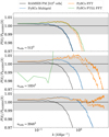 |
Fig. 6 Ratio of the power spectrum with respect to RAMSES (with AMR). In black lines we show results for RAMSES PM (no AMR), while in blue, orange and green we show results for PySCo using multigrid, FFT and FULL_FFT solvers respectively. In top, middle and bottom panels we use 5123, 10243 and 20483 cells respectively for PySCo. In dashed and solid lines we plot results using five- and seven-point gradient operator. The grey shaded area show the ±1% limits. We use TSC in any case, and we do not plot FULL_FFT for ncells = 20483. |
4.3 f(R) gravity
In this section, we validate the implementation of the f (R) gravity model from Hu & Sawicki (2007) described in Section 2.5. To assess this, we run f (R) simulations with varying fR0 values, along with a reference Newtonian simulation. Furthermore, because f (R) corrections are irrelevant at very high redshifts, we use the same Newtonian initial conditions in both cases. In Fig. 8, we compare the power spectrum boost from PySCo with the e-MANTIS emulator (Sáez-Casares et al. 2024), which is based on the ECOSMOG code (Li et al. 2012), itself a modified version of RAMSES. The results show excellent agreement between PySCo and e-MANTIS up to k ~ 1 h Mpc–1. The agreement improves further for higher ncells, except in the case of |fR0| = 10–6, where the curves for PySCo overlap when using FFT. This indicates that PySCo converges well towards the e-MANTIS predictions. Notably, the best agreement is found when using the multigrid solver for | fR0| = 10–4 and 10–5, while FFT performs better for |fR0| = 10–6. This last behaviour could be explained by the multigrid PM solver struggling to accurately compute small-scale features of the scalaron field, as lower values of |fR0| result in sharper transitions between Newtonian and modified gravity regimes. No noticeable impact from the gradient order is observed in any of the cases.
In summary, PySCo demonstrates excellent agreement with e-MANTIS, aligning with prior validation efforts against other codes for similar tests, such as those conducted by Euclid Collaboration: Adamek et al. (2025). For this setup, using the multigrid solver for the Newtonian part seems advantageous for consistency, given that its non-linear version is already employed for the additional f (R) field without approximations.
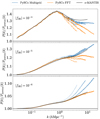 |
Fig. 8 Power spectrum boost from f (R) gravity w.r.t. to the Newtonian case. Blue and orange lines refer respectively to multigrid and FFT Poisson solvers with PySCo (in any case, the scalaron field equation is solved with non-linear multigrid), while black lines show the e-MANTIS emulator. In dotted, dashed and solid lines we use ncells = 5123, 10243 and 20483. Top, middle and bottom panels have the values |fR0| = 10–4, 10–5 and 10–6. In any case we use a seven-point gradient operator. |
4.4 Parametrised gravity
The focus here shifts to simulations with parametrised gravity, where deviations from Newtonian gravity are governed by a single parameter, µ0, representing the gravitational coupling today (as discussed in Section 2.4). In Fig. 9, the power spectrum boost is shown for various values of µ0 compared to a Newtonian simulation. On large scales, the power spectrum ratio approaches unity, which aligns with expectations since the power spectrum is rescaled at the initial redshift according to µ0 (detailed in Appendix A). On smaller scales, the behaviour changes: negative values of µ0 result in a suppression of power, while positive values lead to an excess of power. The magnitude of these deviations increases with larger |µ0|, and the asymmetry between positive and negative values becomes evident. For instance, the departure from Newtonian behaviour is around 60% for µ0 = –0.5 and around 40% for µ0 = 0.5.
There is a slight discrepancy between the results of the FFT and multigrid solvers for larger values of |µ0|, although no significant impact from the gradient stencil order or the number of cells is observed at the same scales.
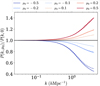 |
Fig. 9 Power spectrum boost from parametrised gravity w.r.t to the Newtonian case (µ0 = 0). Coloured lines refer to different values of µ0, while solid and dashed lines indicates the use of FFT and multigrid solvers respectively. |
4.5 MOND
This section discusses the testing of the MOND implementation within PySCo. MOND was originally proposed as an alternative explanation for dark matter, modifying Newton’s gravitational law in low-acceleration regimes. However, for validation purposes, the same cosmological parameters and initial conditions from Section 4.2 are used, rather than the typical MOND universe with Ωm = Ωb as the goal is to test the MOND gravity solver. The results are illustrated in Fig. 10. The MOND power spectra are noticeably higher than the Newtonian reference. This result aligns with known characteristics of MOND, which accelerates structure formation (Sanders 2001; Nusser 2002), explaining why MOND simulations are usually initialised with lower values of As (or σ8) (Knebe & Gibson 2004; Llinares et al. 2008). To validate the MOND implementation, it is compared to the PoR (Phantom of RAMSES) code (Lüghausen et al. 2015), a MOND patch for RAMSES that uses the simple interpolating function from Equation (14). The agreement between PoR and PySCo is excellent for scales k ~ 1 h/Mpc.
The discrepancies observed at small scales stem from differences between the PM and PM-AMR solvers, a pattern also seen in Fig. 5. Furthermore, the impact of the interpolating function on the power spectrum follows the same trend as observed in Fig. 2. For consistency, we also verified that MOND power spectra converge towards the Newtonian case when g0 ≪ 10−10 m s−2.
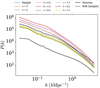 |
Fig. 10 Power spectra for several MOND interpolating functions and parameters (in coloured lines). In back solid line we show the Newtonian counterpart, while the black dashed line refers to a MOND run with the simple parametrisation using the code Phantom of RAMSES. For MOND simulations we use g0 = 10−10 m s−2 and N = 0. In PySCo, we use the multigrid solver in any case. |
4.6 Performances
Finally, we present performance metrics for PySCo on the Adastra supercomputer at CINES, using AMD Genoa EPYC 9654 processors. For FFT-based methods, the PyFFTW package3, a Python wrapper for the FFTW library (Frigo & Johnson 2005), was used. All performance tests were run five times, and the median timings were taken to avoid outliers from potential node-related issues.
The first benchmark focuses on the time required to compute a single time step, as shown in Fig. 11. In a simulation with 5123 particles and cells, the computation takes between 15 to 25 seconds on a single CPU for the various solvers, with the multigrid solver being the fastest and the FULL_FFT solver being the slowest. The force computation using a seven-point gradient from the gravitational potential grid contributes minimally to the overall runtime. Since the multigrid solver outperforms FFT_7pt with similar accuracy, the latter will not be used in the remainder of the paper.
Fig. 12 illustrates the strong scaling efficiency of PySCo’s FFT and multigrid solvers. The scaling improves as the number of cells increases, suggesting that the workload per CPU becomes more efficient with larger grids. For smaller grids (ncells = 1283), the multithreading is less effective, whereas for larger grids (ncells = 10243), multigrid reaches an efficiency of roughly 90% with 64 CPUs. Overall, multigrid consistently exhibits better efficiency than FFTW.
When analysing the total time per time step, a slightly different picture emerges. Efficiency still improves with larger grids but is generally lower than solver-only performance. For smaller grids (ncells = 1283 and 2563), there is little difference between multigrid and FFT, indicating that particle-grid interactions are the primary factor influencing performance, as 5123 particles were used in all cases. A significant drop in efficiency occurs when using fewer than four CPUs, which is followed by a more gradual decline. This is caused by race conditions in the TSC algorithm, where multiple threads attempt to write to the same element in the density grid. To address this, atomic operations were implemented to ensure thread-safe modifications, but these operations slow the mass-assignment process by a factor of four4. Hence, when NCPU < 4 we use the sequential TSC version (which thus does not scale at all by definition), and the parallel-safe version for NCPU ≥ 4, thus giving a better scaling afterwards.
For grids with ncells = 5123, FFT achieves better efficiency than multigrid because, while multigrid is more efficient as a solver, it constitutes a smaller portion of the overall runtime. However, with larger grids ncells = 10243 , the efficiency aligns more closely with the solver-only case, as the solver dominates the runtime. Efficiency reaches approximately 50% for FFT and 75% for multigrid. To ensure optimal efficiency, the number of grid cells should thus be at least eight times the number of particles ncells ≥ 8npart .
For comparison, a full simulation for PySCo with 5123 particles and as many cells takes roughly 0.8 CPU hours for ∼200 time steps, while a RAMSES run with the same setup and AMR enabled takes roughly 3000 CPU hours for ∼1000 time steps.
 |
Fig. 11 Time to compute one time step of a Newtonian simulation for different solvers. In blue, orange, green and red we highlight the time needed to compute a density grid using TSC, an inverse TSC to interpolate the force from grid to particles, a seven-point gradient and the solver respectively. The FULL_FFT method directly computes the force with the kernel described in Eq. (106), hereby removing the need for a finite-derivative gradient part. All timings were done using a single CPU. |
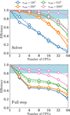 |
Fig. 12 Strong scaling efficiency for the solver only (top panel) and full time step (bottom panel). The solid and dashed lines refer to FFT and multigrid solvers respectively. The efficiency is computed as the time ratio for one CPUs w.r.t N CPUs, divided by N. An efficiency equal to unity denotes perfect parallel scaling. |
5 Conclusions
In this paper, we presented PySCo, a fast particle-mesh N-body code designed for Newtonian and modified-gravity cosmological simulations. PySCo currently supports the f (R) gravity model (Hu & Sawicki 2007), the quasi-linear formulation of MOND (Milgrom 2010), and a time-dependent modification of the gravitational constant via a parameterised model. The code includes multiple solvers, such as multigrid and several FFT methods, each with exact or approximated kernels. We validated PySCo against RAMSES (using multigrid and no AMR), the e-MANTIS emulator for f (R) gravity and Phantom of RAMSES for MOND, and found overall good agreement. The main conclusions of our study are the following:
The TSC mass assignment should be preferred over CIC. CIC leads to larger scatters in the power spectrum and inaccuracies, particularly with FFT solvers when the number of cells exceeds the number of particles;
Three-point gradient operators result in a loss of power at small scales. Using at least a five-point gradient is recommended for better accuracy;
Seven-point Laplacian operators, whether used in multigrid (configuration space) or FFT_7pt (Fourier space), cause power suppression at small scales. Multigrid is favoured because it provides undistinguishable results from FFT_7pt, while being faster and more efficient in parallel computing;
The FFT solver (using the exact Laplacian kernel) is a solid choice overall, especially with TSC instead of CIC when the number of cells exceeds the number of particles;
The FULL_FFT solver is too simplistic to be trusted, except in configurations where the number of cells matches the number of particles (ncells = npart) and TSC is used;
Resolving small scales sufficiently is critical for obtaining a power spectrum at z = 0 that is relatively insensitive to the initial redshift. Otherwise, there will be bias at small scales. Solutions include increasing the resolution (for example, reducing box size), using a higher-order gradient operator, or applying an exact Laplacian operator;
When small scales are well-resolved, the power spectrum at z = 0 becomes insensitive to the starting redshift at around 0.1% for initial redshifts greater than 125, 30, and 10 for 1LPT, 2LPT, and 3LPT, respectively;
We recommend running PySCo with ncells = 8npart for optimal efficiency. Increasing to ncells = 64npart would significantly raise the runtime, contradicting the main advantage of PM-only simulations, which is precisely to be faster than AMR or tree codes;
For standalone simulations, the FFT solver is ideal, as it aligns best with PM-AMR results. For calculating boost factors, such as f (R) simulations against Newtonian ones, multigrid is a faster option, with power losses at small scales cancelling out.
In this paper, we focused on power spectrum, but it would be also possible to compute accurate boost factors for halo mass functions (HMF), as in Euclid Collaboration: Adamek et al. (2025), although the HMF itself (not the boost) is very sensitive to small scales.
PySCo is usable both through command line and as a Python package. It also includes a wide range of built-in utilities, such as initial condition generators and power spectrum estimators. To minimise third-party dependencies, PySCo integrates several in-house modules for particle and mesh algorithms.
In the future, we will port PySCo to GPUs using Numba for CUDA kernels. However, there is currently no plan to implement MPI parallelisation, as the typical PM use case involves small, fast simulations on a single node. PySCo is particularly interesting because it comes with the fast development speed of Python and C/Fortran-like performance. Compared to PM-AMR codes like RAMSES, PySCo offers a dramatic reduction in runtime—potentially simulating in roughly 1/1000th of the time, albeit with less accuracy on small scales. These features make it useful for producing emulators, generating covariance matrices, and training neural networks for upcoming cosmological surveys without requiring massive computational resources. Our aim is to expand PySCo to include a wider range of gravity theories and non-standard dark sector components, creating a versatile framework for exploring cosmological phenomena and aiding in the development of observational constraints.
Acknowledgements
I would like to thank Yann Rasera, Iñigo Sáez-Casares and Himanish Ganjoo for comments on the draft and testing a preliminary version of PySCo. I am also grateful to Stéphane Colombi and Oliver Hahn for insightful discussions regarding initial conditions, as well as Hans Winther on modified gravity simulations and Claudio Llinares for interesting prospects with MOND. I thank Jorge Carretero and Pau Tallada, whose work on the SciPic package convinced me of the viability of Python for performant scientific computing. This project was provided with computer and storage resources by GENCI at CINES thanks to the grant 2023-A0150402287 on the supercomputer Adastra’s GENOA partition.
Appendix A Growth factors
Under the Lagrangian formulation of perturbation theory, the position of tracers at some given time and position is given by
 (A.1)
(A.1)
with q an initial position and Ψ(q, η) a displacement field. The Euler equation is then
 (A.2)
(A.2)
which, when taking the gradient, yields
![Mathematical equation: ${\nabla _{\bf{x}}}\left[ {{{{{\rm{d}}^2}{\bf{x}}} \over {{\rm{d}}{\eta ^2}}} + {\cal H}{{{\rm{d}}{\bf{x}}} \over {{\rm{d}}\eta }}} \right] = - {3 \over 2}{{\cal H}^2}{\Omega _m}(\eta )\delta ({\bf{x}},\eta ).$](/articles/aa/full_html/2025/03/aa52770-24/aa52770-24-eq164.png) (A.3)
(A.3)
Mass conservation imposes ![Mathematical equation: $\bar \rho (\eta ){{\rm{d}}^3}{\bf{q}} = \bar \rho (\eta )[1 + \delta ({\bf{x}},\eta )]{{\rm{d}}^3}{\bf{x}}$](/articles/aa/full_html/2025/03/aa52770-24/aa52770-24-eq165.png) , meaning that ∇x = J−1∇q, with J(q, η) = det [δij + Ψij(q, η)] where δij is a Kronecker Delta. We compute the time evolution of growth factors through the general equation (Jeong 2010)
, meaning that ∇x = J−1∇q, with J(q, η) = det [δij + Ψij(q, η)] where δij is a Kronecker Delta. We compute the time evolution of growth factors through the general equation (Jeong 2010)
![Mathematical equation: $J{\nabla _x}\left[ {{{{{\rm{d}}^2}{\bf{x}}} \over {{\rm{d}}{\eta ^2}}} + {\cal H}{{{\rm{d}}{\bf{x}}} \over {{\rm{d}}\eta }}} \right] = {3 \over 2}{{\cal H}^2}{\Omega _m}(\eta )[J - 1].$](/articles/aa/full_html/2025/03/aa52770-24/aa52770-24-eq166.png) (A.4)
(A.4)
A perturbative expansion at third order gives (Rampf & Buchert 2012)
 (A.5)
(A.5)
![Mathematical equation: $\matrix{ {J({\bf{q}},\eta ) = 1 + \varepsilon D(\eta )\mu _1^{(1)}({\bf{q}}) + {\varepsilon ^2}\left[ {E(\eta )\mu _1^{(2)}({\bf{q}}) + {D^2}(\eta )\mu _2^{(1)}({\bf{q}})} \right]} \cr { + {\varepsilon ^3}\left[ {F(\eta )\mu _1^{(3)}({\bf{q}}) + 2D(\eta )E(\eta )\mu _2^{(1,2)}({\bf{q}}) + {D^3}(\eta )\mu _3^{(1)}({\bf{q}})} \right]} \cr { + O\left( {{\varepsilon ^4}} \right),} \cr } $](/articles/aa/full_html/2025/03/aa52770-24/aa52770-24-eq168.png) (A.6)
(A.6)
with D ≡ D(1), E ≡ D(2) and F ≡ D(3) are the first, second and third-order growth factors respectively, ε ≪ 1 and
 (A.7)
(A.7)
![Mathematical equation: $\mu _2^{(n,m)}(q) = {1 \over 2}\left[ {\Psi _{i,i}^{(n)}(q)\Psi _{j,j}^{(m)}(q) - \Psi _{i,j}^{(n)}(q)\Psi _{j,i}^{(m)}(q)} \right],$](/articles/aa/full_html/2025/03/aa52770-24/aa52770-24-eq170.png) (A.8)
(A.8)
![Mathematical equation: $\mu _3^{(n)}(q) = \det \left[ {\Psi _{i,j}^{(n)}(q)} \right].$](/articles/aa/full_html/2025/03/aa52770-24/aa52770-24-eq171.png) (A.9)
(A.9)
Eq. (A.4) then becomes
![Mathematical equation: $J\left[ {{\delta _{ij}} - {\Psi _{i,j}}} \right]\left[ {{{{{\rm{d}}^2}{\Psi _{i,j}}} \over {{\rm{d}}{\eta ^2}}} + {\cal H}{{{\rm{d}}{\Psi _{i,j}}} \over {{\rm{d}}\eta }}} \right] = {3 \over 2}{{\cal H}^2}{\Omega _m}(\eta )[J - 1],$](/articles/aa/full_html/2025/03/aa52770-24/aa52770-24-eq172.png) (A.10)
(A.10)
with ∂/∂xi = [δij + Ψi,j]−1 ∂/∂qj and [δij + Ψi,j]−1 ≈ [δij − Ψi,j].
- The first-order solution (Zel’dovich 1970) is
 (A.11)
with  . where D ≡ D+ the first-order growth factor, and
  .
.
- The second-order solution is then
![Mathematical equation: $\mathop E\limits^ + {\cal H}\dot E - \beta \left[ {E - {D^2}} \right] = 0.$](/articles/aa/full_html/2025/03/aa52770-24/aa52770-24-eq176.png) (A.12)
(A.12)
- The third-order solutions are given by
![Mathematical equation: $\matrix{ {[\mathop F\limits^ + {\cal H}\dot F - \beta F]\mu _1^{(3)}} \hfill \cr { + 2[D\mathop E\limits^ + {\cal H}D\dot E + \mathop D\limits^ E + {\cal H}E\dot E - \beta DE]\mu _2^{(1,2)}} \hfill \cr { + \left[ {3\mathop D\limits^ {D^2} + 3{\cal H}\dot D{D^2} - \beta {D^3}} \right]\mu _3^{(1)} = 0,} \hfill \cr } $](/articles/aa/full_html/2025/03/aa52770-24/aa52770-24-eq177.png) (A.13)
(A.13)
which give rise to two tangential and one transversal modes. Their ordinary differential equations (ODEs) are given by
![Mathematical equation: ${\mathop F\limits^ _a} + {\cal H}{\dot F_a} - \beta \left[ {{F_a} - 2{D^3}} \right] = 0,$](/articles/aa/full_html/2025/03/aa52770-24/aa52770-24-eq178.png) (A.14)
(A.14)
![Mathematical equation: ${\mathop F\limits^ _b} + {\cal H}{\dot F_b} - \beta \left[ {{F_b} - D\left( {E - {D^2}} \right)} \right] = 0,$](/articles/aa/full_html/2025/03/aa52770-24/aa52770-24-eq179.png) (A.15)
(A.15)
![Mathematical equation: ${\mathop F\limits^ _c} + {\cal H}[\dot ED - E\dot D] + \beta {D^3} = 0,$](/articles/aa/full_html/2025/03/aa52770-24/aa52770-24-eq180.png) (A.16)
(A.16)
where the last equation can be derived using the equation for irrotational fluids (Catelan 1995). In practice, we implement these ODEs as functions of In(a), leading to the following set of equations
 (A.17)
![Mathematical equation: $E'' = - \gamma E' + \beta \left[ {E - {D^2}} \right],$](/articles/aa/full_html/2025/03/aa52770-24/aa52770-24-eq182.png) (A.18)
(A.18)
![Mathematical equation: ${F''_a} = - \gamma {F'_a} + \beta \left[ {{F_a} - 2{D^3}} \right],$](/articles/aa/full_html/2025/03/aa52770-24/aa52770-24-eq183.png) (A.19)
(A.19)
![Mathematical equation: ${F''_b} = - \gamma {F'_b} + \beta \left[ {{F_b} - 2D\left( {E - {D^2}} \right)} \right],$](/articles/aa/full_html/2025/03/aa52770-24/aa52770-24-eq184.png) (A.20)
(A.20)
 (A.21)
with D′= dD/d ln a and
 (A.22)
![Mathematical equation: $\gamma = {1 \over 2}\left\{ {1 - 3{\Omega _\Lambda }(a)\left[ {{w_0} + {w_a}(1 - a)} \right] - {\Omega _r}(a)} \right\}.$](/articles/aa/full_html/2025/03/aa52770-24/aa52770-24-eq187.png) (A.23)
(A.23)
The nth-order growth factors can be estimated through f(n) = D(n)′/D(n). It is straightforward to implement a scaleindependent parametrised form of modified gravity (as in Section 2.4) by making the small change β = 3µ(a)Ωm(a)/2.
Approximated analytical solutions for the growing mode in a matter-dominated era (and neglecting radiation) are (Catelan 1995; Rampf & Buchert 2012)
 (A.24)
 (A.25)
 (A.26)
 (A.27)
Approximated fits with dependence on Ωm for the growth factors and growth rates are also available in Bouchet et al. (1995).
Appendix B Initial conditions
Appendix B.1 Time stepping
As described in Section 3.4, we use two kinds of time stepping criteria, one based on cosmological time (in RAMSES, the scale factor cannot change by more than 10% in a single time step), and another based on the free-fall time (acceleration) or maximum velocity compared to the mesh size. For the latter two we also use a Courant-like factor, which multiplies the final time step and is equal to 0.8 by default.
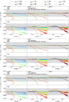 |
Fig. B.1 Same as Fig. 3, but using a seven-point gradient and varying the maximal scale factor variation in the cosmological time criterion, from top to bottom. |
While small changes in the Courant factor do not significantly affect the results, using a time step that is too large can introduce a scale-independent bias in the power spectrum at redshift z = 0, as shown in Fig. B.1. We observe a bias of approximately 0.3% in the power spectrum at k ~ 0.1 h−1 Mpc when the time step allows for a 10% maximum variation in the scale factor. This bias decreases to about 0.1% with a 5% variation and seems negligible when using variations below 3%. To ensure accuracy and avoid such biases, we used a more conservative 2% variation in scale factor by default. Additionally, we note that while 1LPT appears to work well on large scales, this is primarily due to the limited box size of the simulation, as we directly see the moment when the power spectrum is damped compared to the reference at initial redshift z = 150.
Appendix B.2 Initial positions
In PySCo, two methods for initialising particle positions were implemented: at cell centres or at cell edges. Given the periodic boundary conditions, these methods should ideally produce no differences due to translational symmetry. However, discrepancies can arise depending on the mass-assignment scheme used. For example, using the nearest grid point (NGP) method, where the density is calculated directly from the number of particles within each grid cell, will produce a uniform density grid if the particles are positioned at cell centres. This is because, at small displacements, each cell would contain exactly one particle. In contrast, if the particles are initialised at the cell edges, the density field can become inhomogeneous, as it depends more strongly on the displacement field. This difference is demonstrated in Fig. B.2, which shows the ratio of the power spectrum for various initial redshifts compared to a reference case where the initial redshift is zini = 150 and particles are initialised at cell edges The results are quite similar to those from Fig. 3, where particles were initialised at cell centres. However, for five- and seven-point gradient operators with 3LPT, a slight bias appears at small scales, with a loss of power even for zini > 10 compared to the reference case. As a result of these findings, we decided to initialise particles at cell centres in the main text.
Appendix C Multigrid convergence
This section presents convergence tests for the multigrid algorithm (detailed in Section 3.7). Fig. C.1 shows the convergence rate of different multigrid cycles (V, F, and W). First, we remark that the convergence rate is nearly independent of redshift. The only redshift-dependent variation is the maximum residual suppression due to numerical roundings, which becomes evident after many iterations. This discrepancy arises from the normalisation by the first-guess residual, which is less accurate at lower redshifts due to the Universe being more structured compared to higher redshifts. Additionally, F and W cycles show very similar behaviour but take approximately 1.9 and 2.1 times longer than V cycles, respectively. Without overrelaxation (ω = 1), F and W cycles reduce the residual by a factor of 100 per iteration, while V cycles achieve a factor of 10 reduction. Overrelaxation with ω = 1.25 significantly improves the convergence rate, although it may not immediately help in the first V cycle due to the initial guess still being inaccurate. In practice, ω = 1.25 is applied for linear Poisson equations, whereas for non-linear cases, ω = 1.0 is used since SOR proves less effective. In Fig. C.1, one Jacobi step was used as the first guess (see Section 3.6), but Table C.1 suggests that using the potential field from the last step can significantly reduce the initial residuals. Further improvements through rescaling this last-step solution using the linear growth factor (discussed in Section 3.9) only offer marginal reductions in the residual. Rescaling becomes more useful at higher redshifts, where time steps are larger. Overall, using the last step as the first guess is a good strategy, sometimes saving one V cycle, though it requires keeping the gravitational potential grid in memory. Rescaling, however, seems unnecessary unless the time steps are particularly large.
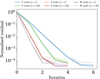 |
Fig. C.1 Convergence rate of multigrid cycles as function of the number of cycles (or iterations). Blue, orange and purple lines refer to V, F and W cycles respectively, while in green, red and grey we use SOR with relaxation parameter ω = 1.25. In solid, dashed and dotted lines we show results at z = 0,1 and 3 respectively. For the first guess we use one Jacobi step, thereby neglecting the information from previous step. |
Ratio of residuals for different first guesses.
The final test concerns the threshold criterion for convergence of the multigrid algorithm. Fig. C.2 shows the power spectrum ratio at z = 0 for different values of a. Even with a very large threshold value, like a = 10, the bias in the power spectrum is only around 0.1%. The results for α = 0.1 and 1 are almost identical, likely because these thresholds are passed within the same V cycle, which typically reduces the residual by a factor of 20–30 per iteration when using SOR. With α = 0.01, the bias drops to less than 0.01%, and convergence is essentially achieved by α = 0.001. These results are consistent regardless of starting redshift, LPT order, or mass-assignment scheme. In practice, an α value of 0.01 is recommended, as it produces highly accurate results without introducing any significant bias, whereas increasing α further results in a small but noticeable decrease in the power spectrum.
 |
Fig. C.2 Power spectrum ratio with varying multigrid threshold parameter a (see Eq. 96) w.r.t to the reference where α = 10−4. In blue, orange, green, red and purple we have α = 0.001,0.01,0.1,1 and 10. The grey shaded area indicates the ±0.1% limits. In any case we use V cycles. |
Appendix D Point-mass test
In this appendix, we evaluate the performance of PySCo in the simplified scenario of a single point mass while maintaining periodic boundary conditions. The normalised gravitational field for a homogeneous and isotropic sphere of radius R is given by
 (D.1)
(D.1)
where r = | r |. To incorporate periodicity, we apply the Ewald summation method (Hernquist et al. 1991). For simplicity, we only account for the contribution from replicas, as in Rácz et al. (2021)
 (D.2)
(D.2)
where a unit simulation box is assumed, n represents integer triplets, and | (r + n) | < 2.6 ensures that the force decays to zero between replicas.
Fig. D.1 illustrates the acceleration of 1283 massless particles surrounding a point mass in a simulation with 643 cells. The radial accelerations closely follow the predictions for the inner sphere at scales below the coarse cell size h. At larger scales, the acceleration transitions to the standard 1/r2 behaviour, albeit with damping due to periodicity. This damping is well captured by Eq. (D.2). Notably, the TSC interpolation scheme demonstrates significantly improved isotropy compared to CIC, as evidenced by lower tangential acceleration values. For the CIC scheme, when the point mass is positioned at a cell centre, only one cell exhibits a non-zero density with a value of ρ0. However, for a point mass located at a cell edge, eight cells have non-zero densities, each with a value of ρ0/8 for CIC and TSC. The sole distinction in this configuration arises from the inverse interpolation from the grid back to the particles. In contrast, for the TSC scheme with the point mass placed at the cell centre, 27 cells exhibit non-zero densities. In terms of solver performance, the results from the FFT_7pt and multigrid solvers are consistent and identical, as expected. While the accelerations align at larger distances, the multigrid and FFT_7pt solvers exhibit a slight overestimation of acceleration at small scales. Put differently, these solvers generate a deeper potential compared to the FFT solver. This increased acceleration results in higher particle velocities, which in turn suppresses clustering at small scales. This behaviour is consistent with the observed damping of the matter power spectrum, as shown in Fig. 6.
 |
Fig. D.1 Acceleration of massless particles randomly sampled around a point mass, as a function of distance. The left and right panels illustrate results using the CIC and TSC mass interpolation (and inverse interpolation) schemes, respectively. The top panels show cases where the point mass is positioned at the centre of a cell, while the bottom panels depict cases where it is placed at the edge of a cell. The red, yellow, and blue data points represent accelerations computed using the FFT solver (uncorrected for the mass-assignment scheme), the FFT_7pt solver, and the multigrid solver, respectively. Circles denote radial acceleration, while triangles indicate tangential acceleration. The black solid line represents the theoretical prediction F(r, h) from Eq. (D.1). For comparison, dotted lines correspond to F(r, rs), where rs = (6/π)1/3 h is the radius of a sphere with the same volume as a cell of size 2h. Dashed lines illustrate the periodic case |

Appendix E Data locality
Finally, we highlight the importance of data locality in particlemesh interactions, focusing on the impact it has on runtime performance. Fig. E.1 illustrates the runtime for the inverse TSC algorithm under different particle array orderings. When the particle array is randomly sorted, the inverse TSC takes approximately 0.45 seconds for the first 100 steps, with a gradual decrease down to ∼0.37 seconds. In a randomly sorted array, consecutive particles are unlikely to be spatially close, leading to a higher number of cache misses because grid elements are also distant in memory. However, as particles cluster at later times, even a randomly sorted array experiences improved performance due to the higher likelihood that two neighbouring particles are closer spatially, reducing cache misses.
 |
Fig. E.1 Runtime of the inverse TSC algorithm (from mesh to particles) for a force field. In coloured lines we show the results with different ordering of the particle arrays. ‘Randomly sorted’ means that in the initial conditions we randomly shuffle the particle positions. ‘Initially sorted only’ means that in the initial conditions the particles are linearly ordered, with the same contiguous properties as the cells they are in. ‘Partially’ and ‘Fully sorted’ means than every N steps (here 50), we sort the particle array according to Morton indexing based on their positions (see Section 3.2). The simulation has 5123 particles and as many cells, and was run with 64 CPUs. |
In contrast, if the particle array is initially sorted, the runtime for inverse TSC starts much lower at ∼0.04 seconds and increases up to ∼0.11 seconds over time. This improvement comes from neighbouring particles in the array being spatially closer at the beginning, allowing the cache to be used more efficiently. The ten-fold improvement in performance, achieved solely by optimising data locality, is a significant gain without requiring complex programming techniques. Over time, as particles move, the initial sorting deteriorates, leading to less efficient cache usage, even though clustering increases.
To maintain performance, PySCo offers the ability to re-sort the particles every N steps (default N = 50, adjustable by the user). With periodic sorting, the ‘fully sorted’ runtime remains flat as a function of time. However, the sorting operation can become a bottleneck, as Numba does not support parallel sorting algorithms, and resorting to sequential sorting is prohibitive for large particle counts. To address this, PySCo implements a parallelised, partial sorting method. The particle array is divided into chunks, with Nchunks = NCPUs , where each chunk is sorted independently by each CPU. The results of this partial sorting are comparable to those of fully sorted arrays, with a slight runtime increase at late times due to the partial nature of the sorting. This increase is marginal, even when using up to 64 CPUs. Therefore, PySCo uses this partial sorting method by default as a balance between performance and computational overhead, especially for large simulations.
References
- Abbott, T. M. C., Abdalla, F. B., Avila, S., et al. 2019, Phys. Rev. D, 99, 123505 [NASA ADS] [CrossRef] [Google Scholar]
- Adamek, J., & Fidler, C. 2019, J. Cosmology Astropart. Phys., 2019, 026 [CrossRef] [Google Scholar]
- Adamek, J., Daverio, D., Durrer, R., & Kunz, M. 2016, JCAP, 7, 053 [CrossRef] [Google Scholar]
- Alam, S., Aubert, M., Avila, S., et al. 2021, Phys. Rev. D, 103, 083533 [NASA ADS] [CrossRef] [Google Scholar]
- Amendola, L., Kunz, M., & Sapone, D. 2008, J. Cosmology Astropart. Phys., 2008, 013 [Google Scholar]
- Angulo, R. E., & Hahn, O. 2022, Liv. Rev. Computat. Astrophys., 8, 1 [CrossRef] [Google Scholar]
- Angulo, R. E., & Pontzen, A. 2016, MNRAS, 462, L1 [NASA ADS] [CrossRef] [Google Scholar]
- Angus, G. W., van der Heyden, K. J., Famaey, B., et al. 2012, MNRAS, 421, 2598 [Google Scholar]
- Astropy Collaboration (Price-Whelan, A. M., et al.) 2022, ApJ, 935, 167 [NASA ADS] [CrossRef] [Google Scholar]
- Bardeen, J. M. 1980, PrD, 22, 1882 [NASA ADS] [Google Scholar]
- Barrera-Hinojosa, C., & Li, B. 2020, J. Cosmology Astropart. Phys., 2020, 007 [Google Scholar]
- Begeman, K. G., Broeils, A. H., & Sanders, R. H. 1991, MNRAS, 249, 523 [Google Scholar]
- Behnel, S., Bradshaw, R., Citro, C., et al. 2011, Comput. Sci. Eng., 13, 31 [Google Scholar]
- Bekenstein, J. 2006, Contemp. Phys., 47, 387 [Google Scholar]
- Bekenstein, J., & Milgrom, M. 1984, ApJ, 286, 7 [NASA ADS] [CrossRef] [Google Scholar]
- Bernardeau, F., Colombi, S., Gaztañaga, E., & Scoccimarro, R. 2002, PhysRep, 367, 1 [Google Scholar]
- Bertschinger, E. 2001, APJS, 137, 1 [NASA ADS] [CrossRef] [Google Scholar]
- Bonvin, C., & Durrer, R. 2011, PrD, 84, 063505 [NASA ADS] [Google Scholar]
- Bose, S., Li, B., Barreira, A., et al. 2017, J. Cosmology Astropart. Phys., 2017, 050 [CrossRef] [Google Scholar]
- Bouchet, F. R., Colombi, S., Hivon, E., & Juszkiewicz, R. 1995, A&A, 296, 575 [NASA ADS] [Google Scholar]
- Breton, M.-A., Rasera, Y., Taruya, A., Lacombe, O., & Saga, S. 2019, MNRAS, 483, 2671 [NASA ADS] [CrossRef] [Google Scholar]
- Buchdahl, H. A. 1970, MNRAS, 150, 1 [NASA ADS] [Google Scholar]
- Buchert, T., & Ehlers, J. 1993, MNRAS, 264, 375 [Google Scholar]
- Burrage, C., & Sakstein, J. 2018, Liv. Rev. Relativ., 21, 1 [Google Scholar]
- Candlish, G. N., Smith, R., & Fellhauer, M. 2015, MNRAS, 446, 1060 [NASA ADS] [CrossRef] [Google Scholar]
- Catelan, P. 1995, MNRAS, 276, 115 [NASA ADS] [Google Scholar]
- Challinor, A., & Lewis, A. 2011, PrD, 84, 043516 [NASA ADS] [Google Scholar]
- Chevallier, M., & Polarski, D. 2001, Int. J. Mod. Phys. D, 10, 213 [Google Scholar]
- Chisari, N. E., & Zaldarriaga, M. 2011, PrD, 83, 123505 [NASA ADS] [Google Scholar]
- Couchman, H. M. P. 1991, APJ, 368, L23 [NASA ADS] [CrossRef] [Google Scholar]
- Crocce, M., Pueblas, S., & Scoccimarro, R. 2006, MNRAS, 373, 369 [NASA ADS] [CrossRef] [Google Scholar]
- Dakin, J., Hannestad, S., & Tram, T. 2022, MNRAS, 513, 991 [CrossRef] [Google Scholar]
- Dvali, G., Gabadadze, G., & Porrati, M. 2000, Phys. Lett. B, 485, 208 [Google Scholar]
- Efstathiou, G., Davis, M., White, S. D. M., & Frenk, C. S. 1985, ApJS, 57, 241 [NASA ADS] [CrossRef] [Google Scholar]
- Euclid Collaboration (Adamek, J., et al.) 2025, A&A, in press, https://doi.org/10.1051/0004-6361/202452180 [Google Scholar]
- Euclid Collaboration (Castander, F. J., et al.) 2025, A&A, in press, https://doi.org/10.1051/0004-6361/202450853 [Google Scholar]
- Famaey, B., & Binney, J. 2005, MNRAS, 363, 603 [NASA ADS] [CrossRef] [Google Scholar]
- Famaey, B., & McGaugh, S. S. 2012, Liv. Rev. Relativ., 15, 10 [Google Scholar]
- Feng, Y., Chu, M.-Y., Seljak, U., & McDonald, P. 2016, MNRAS, 463, 2273 [NASA ADS] [CrossRef] [Google Scholar]
- Fidler, C., Rampf, C., Tram, T., et al. 2015, PrD, 92, 123517 [NASA ADS] [Google Scholar]
- Fidler, C., Tram, T., Rampf, C., et al. 2016, JCAP, 9, 031 [Google Scholar]
- Frigo, M., & Johnson, S. G. 2005, Proc. IEEE, 93, 216 [Google Scholar]
- Frusciante, N., & Perenon, L. 2020, Phys. Rep., 857, 1 [NASA ADS] [CrossRef] [Google Scholar]
- Garrison, L. H., Eisenstein, D. J., Ferrer, D., Maksimova, N. A., & Pinto, P. A. 2021, MNRAS, 508, 575 [NASA ADS] [CrossRef] [Google Scholar]
- Green, S. R., & Wald, R. M. 2014, Class. Quant. Grav., 31, 234003 [NASA ADS] [CrossRef] [Google Scholar]
- Guillet, T., & Teyssier, R. 2011, J. Computat. Phys., 230, 4756 [NASA ADS] [CrossRef] [Google Scholar]
- Hahn, O., & Abel, T. 2013, Astrophysics Source Code Library [record ascl:1311.011] [Google Scholar]
- Harris, C. R., Millman, K. J., van der Walt, S. J., et al. 2020, Nature, 585, 357 [NASA ADS] [CrossRef] [Google Scholar]
- Hassani, F., & Lombriser, L. 2020, MNRAS, 497, 1885 [NASA ADS] [CrossRef] [Google Scholar]
- Hernquist, L., Bouchet, F. R., & Suto, Y. 1991, ApJS, 75, 231 [NASA ADS] [CrossRef] [Google Scholar]
- Hernández-Aguayo, C., Ruan, C.-Z., Li, B., et al. 2022, J. Cosmol. Astropart. Phys., 2022, 048 [Google Scholar]
- Hockney, R. W., & Eastwood, J. W. 1981, Computer Simulation Using Particles (New York: McGraw-Hill) [Google Scholar]
- Hu, W., & Sawicki, I. 2007, Phys. Rev. D, 76, 064004 [CrossRef] [Google Scholar]
- Ishiyama, T., Fukushige, T., & Makino, J. 2009, PASJ, 61, 1319 [NASA ADS] [CrossRef] [Google Scholar]
- Ishiyama, T., Prada, F., Klypin, A. A., et al. 2021, MNRAS, 506, 4210 [NASA ADS] [CrossRef] [Google Scholar]
- Jeong, D. 2010, PhD thesis, University of Texas, Austin, USA [Google Scholar]
- Jing, Y. P. 2005, ApJ, 620, 559 [NASA ADS] [CrossRef] [Google Scholar]
- Khoury, J., & Weltman, A. 2004, Phys. Rev. Lett., 93, 171104 [NASA ADS] [CrossRef] [Google Scholar]
- Klypin, A., & Prada, F. 2018, MNRAS, 478, 4602 [NASA ADS] [CrossRef] [Google Scholar]
- Knebe, A., & Gibson, B. K. 2004, MNRAS, 347, 1055 [NASA ADS] [CrossRef] [Google Scholar]
- Knebe, A., Green, A., & Binney, J. 2001, MNRAS, 325, 845 [NASA ADS] [CrossRef] [Google Scholar]
- Kravtsov, A. V., Klypin, A. A., & Khokhlov, A. M. 1997, APJS, 111, 73 [NASA ADS] [CrossRef] [Google Scholar]
- Lam, S. K., Pitrou, A., & Seibert, S. 2015, in Proceedings of the Second Workshop on the LLVM Compiler Infrastructure in HPC, 1 [Google Scholar]
- Lewis, A., Challinor, A., & Lasenby, A. 2000, ApJ, 538, 473 [Google Scholar]
- Li, B., Zhao, G.-B., Teyssier, R., & Koyama, K. 2012, JCAP, 1, 051 [Google Scholar]
- Linder, E. V. 2003, Phys. Rev. Lett., 90, 091301 [Google Scholar]
- List, F., Hahn, O., & Rampf, C. 2024, Phys. Rev. Lett., 132, 131003 [Google Scholar]
- Llinares, C. 2018, Int. J. Mod. Phys. D, 27, 1848003 [Google Scholar]
- Llinares, C., Knebe, A., & Zhao, H. 2008, MNRAS, 391, 1778 [NASA ADS] [CrossRef] [Google Scholar]
- Llinares, C., Mota, D. F., & Winther, H. A. 2014, A&A, 562, A78 [NASA ADS] [CrossRef] [EDP Sciences] [Google Scholar]
- Lüghausen, F., Famaey, B., & Kroupa, P. 2015, Can. J. Phys., 93, 232 [CrossRef] [Google Scholar]
- Ma, C.-P., & Bertschinger, E. 1995, ApJ, 455, 7 [NASA ADS] [CrossRef] [Google Scholar]
- Martel, H., & Shapiro, P. R. 1998, MNRAS, 297, 467 [Google Scholar]
- Merz, H., Pen, U.-L., & Trac, H. 2005, New Astron., 10, 393 [CrossRef] [Google Scholar]
- Michaux, M., Hahn, O., Rampf, C., & Angulo, R. E. 2021, MNRAS, 500, 663 [Google Scholar]
- Milgrom, M. 1983, ApJ, 270, 365 [Google Scholar]
- Milgrom, M. 2009, Phys. Rev. D, 80, 123536 [NASA ADS] [CrossRef] [Google Scholar]
- Milgrom, M. 2010, MNRAS, 403, 886 [NASA ADS] [CrossRef] [Google Scholar]
- Milgrom, M. 2023, Phys. Rev. D, 108, 084005 [NASA ADS] [CrossRef] [Google Scholar]
- Milgrom, M., & Sanders, R. H. 2008, ApJ, 678, 131 [NASA ADS] [CrossRef] [Google Scholar]
- Nusser, A. 2002, MNRAS, 331, 909 [NASA ADS] [CrossRef] [Google Scholar]
- Orszag, S. A. 1971, J. Atmos. Sci., 28, 1074 [NASA ADS] [CrossRef] [Google Scholar]
- Oyaizu, H. 2008, Phys. Rev. D, 78, 123523 [NASA ADS] [CrossRef] [Google Scholar]
- Peebles, P. J. E. 1980, The large-scale structure of the universe (Princeton University Press) [Google Scholar]
- Pen, U.-L. 1997, ApJ, 490, L127 [NASA ADS] [CrossRef] [Google Scholar]
- Planck Collaboration XIV. 2016, A&A, 594, A14 [NASA ADS] [CrossRef] [EDP Sciences] [Google Scholar]
- Planck Collaboration VI. 2020, A&A, 641, A6 [NASA ADS] [CrossRef] [EDP Sciences] [Google Scholar]
- Potter, D., Stadel, J., & Teyssier, R. 2017, Computational Astrophys. Cosmol., 4, 2 [Google Scholar]
- Press, W. H., Teukolsky, S. A., Vetterling, W. T., & Flannery, B. P. 1992, Numerical Recipes in C, 2nd edn. (Cambridge, USA: Cambridge University Press) [Google Scholar]
- Prunet, S., Pichon, C., Aubert, D., et al. 2008, ApJs, 178, 179 [NASA ADS] [CrossRef] [Google Scholar]
- Puchwein, E., Baldi, M., & Springel, V. 2013, MNRAS, 436, 348 [NASA ADS] [CrossRef] [Google Scholar]
- Rácz, G., Szapudi, I., Csabai, I., & Dobos, L. 2021, MNRAS, 503, 5638 [CrossRef] [Google Scholar]
- Rampf, C., & Buchert, T. 2012, J. Cosmology Astropart. Phys., 2012, 021 [Google Scholar]
- Rampf, C., List, F., & Hahn, O. 2025, J. Cosmology Astropart. Phys., 2025, 020 [Google Scholar]
- Rasera, Y., Breton, M. A., Corasaniti, P. S., et al. 2022, A&A, 661, A90 [NASA ADS] [CrossRef] [EDP Sciences] [Google Scholar]
- Riess, A. G., Yuan, W., Macri, L. M., et al. 2022, ApJ, 934, L7 [NASA ADS] [CrossRef] [Google Scholar]
- Ruan, C.-Z., Hernández-Aguayo, C., Li, B., et al. 2022, J. Cosmology Astropart. Phys., 2022, 018 [CrossRef] [Google Scholar]
- Sáez-Casares, I., Rasera, Y., & Li, B. 2024, MNRAS, 527, 7242 [Google Scholar]
- Sanders, R. H. 2001, ApJ, 560, 1 [NASA ADS] [CrossRef] [Google Scholar]
- Scoccimarro, R. 1998, MNRAS, 299, 1097 [NASA ADS] [CrossRef] [Google Scholar]
- Simpson, F., Heymans, C., Parkinson, D., et al. 2013, MNRAS, 429, 2249 [Google Scholar]
- Sirko, E. 2005, ApJ, 634, 728 [NASA ADS] [CrossRef] [Google Scholar]
- Skordis, C., & Złosnik, T. 2021, Phys. Rev. Lett., 127, 161302 [NASA ADS] [CrossRef] [Google Scholar]
- Sotiriou, T. P., & Faraoni, V. 2010, Rev. Mod. Phys., 82, 451 [NASA ADS] [CrossRef] [Google Scholar]
- Springel, V., Pakmor, R., Zier, O., & Reinecke, M. 2021, MNRAS, 506, 2871 [NASA ADS] [CrossRef] [Google Scholar]
- Teyssier, R. 2002, A&A„ 385, 337 [Google Scholar]
- Valogiannis, G., & Bean, R. 2017, Phys. Rev. D, 95, 103515 [CrossRef] [Google Scholar]
- Villaescusa-Navarro, F. 2018, Pylians: Python libraries for the analysis of numerical simulations, Astrophysics Source Code Library [record ascl:1811.008] [Google Scholar]
- Visser, P. M., Eijt, S. W. H., & de Nijs, J. V. 2024, A&A, 681, A90 [NASA ADS] [CrossRef] [EDP Sciences] [Google Scholar]
- Vogt, S. M. L., Bocquet, S., Davies, C. T., et al. 2025, Phys. Rev. D, 111, 043519 [NASA ADS] [CrossRef] [Google Scholar]
- Winther, H. A., Schmidt, F., Barreira, A., et al. 2015, MNRAS, 454, 4208 [NASA ADS] [CrossRef] [Google Scholar]
- Winther, H. A., Koyama, K., Manera, M., Wright, B. S., & Zhao, G.-B. 2017, J. Cosmol. Astropart. Phys., 2017, 006 [CrossRef] [Google Scholar]
- Yoo, J., Fitzpatrick, A. L., & Zaldarriaga, M. 2009, PrD, 80, 083514 [NASA ADS] [Google Scholar]
- Zel’dovich, Y. B. 1970, A&A, 5, 84 [NASA ADS] [Google Scholar]
While RAMSES converts to cm.
Unfortunately, Numba does not currently contain a way to deal with race conditions on CPUs natively. We thus had to rely on a modified version of atomic operations developed in https://github.com/KatanaGraph/katana. We will move on the official implementation of Numba atomics once they are developed.
All Tables
All Figures
|
Fig. 1 Pseudo code in Python for the multigrid V-cycle algorithm. We highlight in cyan the lines where the theory of gravitation enters. |
| In the text | |
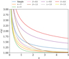 |
Fig. 2 MOND interpolating functions for the different families and parameters shown in Sect. 2.3. |
| In the text | |
|
Fig. 3 Ratio of the matter power spectrum at z = 0 for different starting redshift zini (in coloured lines), with respect to a reference simulation with zini = 150. We use 1LPT, 2LPT or 3LPT initial conditions from left to right and three-, five- and seven-point gradients from top to bottom panels. We use the FFT solver in any case (see Section 3.8). In each subplot the top and bottom panels show simulations which use TSC and CIC mass-assignments schemes respectively. Grey shaded area denotes a 1% discrepancy w.r.t. the reference power spectrum. |
| In the text | |
|
Fig. 4 Same as Fig. 3, but varying the N-body solver instead of gradient order, which is kept to seven-point (except for the FULL_FFT solver which does not make use of finite gradients). |
| In the text | |
|
Fig. 5 Top panel: ratio of the power spectrum for three-, five- and seven-point gradient in blue, orange and green lines respectively using multigrid, with respect to RAMSES (with AMR disabled and also using multigrid). Because RAMSES does not stop exactly at z = 0 we rescaled its power spectrum the linear growth factor. The grey shaded area show the ±1% limits. Bottom panel: ratio of the power spectrum using the PySCo FFT_7pt solver w.r.t PySCo multigrid. The dark grey shaded area show the 10–5 limits. In any case we use a TSC algorithm. |
| In the text | |
|
Fig. 6 Ratio of the power spectrum with respect to RAMSES (with AMR). In black lines we show results for RAMSES PM (no AMR), while in blue, orange and green we show results for PySCo using multigrid, FFT and FULL_FFT solvers respectively. In top, middle and bottom panels we use 5123, 10243 and 20483 cells respectively for PySCo. In dashed and solid lines we plot results using five- and seven-point gradient operator. The grey shaded area show the ±1% limits. We use TSC in any case, and we do not plot FULL_FFT for ncells = 20483. |
| In the text | |
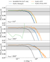 |
Fig. 7 Same as Fig. 6 but using CIC. |
| In the text | |
|
Fig. 8 Power spectrum boost from f (R) gravity w.r.t. to the Newtonian case. Blue and orange lines refer respectively to multigrid and FFT Poisson solvers with PySCo (in any case, the scalaron field equation is solved with non-linear multigrid), while black lines show the e-MANTIS emulator. In dotted, dashed and solid lines we use ncells = 5123, 10243 and 20483. Top, middle and bottom panels have the values |fR0| = 10–4, 10–5 and 10–6. In any case we use a seven-point gradient operator. |
| In the text | |
|
Fig. 9 Power spectrum boost from parametrised gravity w.r.t to the Newtonian case (µ0 = 0). Coloured lines refer to different values of µ0, while solid and dashed lines indicates the use of FFT and multigrid solvers respectively. |
| In the text | |
|
Fig. 10 Power spectra for several MOND interpolating functions and parameters (in coloured lines). In back solid line we show the Newtonian counterpart, while the black dashed line refers to a MOND run with the simple parametrisation using the code Phantom of RAMSES. For MOND simulations we use g0 = 10−10 m s−2 and N = 0. In PySCo, we use the multigrid solver in any case. |
| In the text | |
|
Fig. 11 Time to compute one time step of a Newtonian simulation for different solvers. In blue, orange, green and red we highlight the time needed to compute a density grid using TSC, an inverse TSC to interpolate the force from grid to particles, a seven-point gradient and the solver respectively. The FULL_FFT method directly computes the force with the kernel described in Eq. (106), hereby removing the need for a finite-derivative gradient part. All timings were done using a single CPU. |
| In the text | |
|
Fig. 12 Strong scaling efficiency for the solver only (top panel) and full time step (bottom panel). The solid and dashed lines refer to FFT and multigrid solvers respectively. The efficiency is computed as the time ratio for one CPUs w.r.t N CPUs, divided by N. An efficiency equal to unity denotes perfect parallel scaling. |
| In the text | |
|
Fig. B.1 Same as Fig. 3, but using a seven-point gradient and varying the maximal scale factor variation in the cosmological time criterion, from top to bottom. |
| In the text | |
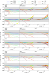 |
Fig. B.2 Same as Fig. 3, but initialising the particles at cell edges. |
| In the text | |
|
Fig. C.1 Convergence rate of multigrid cycles as function of the number of cycles (or iterations). Blue, orange and purple lines refer to V, F and W cycles respectively, while in green, red and grey we use SOR with relaxation parameter ω = 1.25. In solid, dashed and dotted lines we show results at z = 0,1 and 3 respectively. For the first guess we use one Jacobi step, thereby neglecting the information from previous step. |
| In the text | |
|
Fig. C.2 Power spectrum ratio with varying multigrid threshold parameter a (see Eq. 96) w.r.t to the reference where α = 10−4. In blue, orange, green, red and purple we have α = 0.001,0.01,0.1,1 and 10. The grey shaded area indicates the ±0.1% limits. In any case we use V cycles. |
| In the text | |
|
Fig. D.1 Acceleration of massless particles randomly sampled around a point mass, as a function of distance. The left and right panels illustrate results using the CIC and TSC mass interpolation (and inverse interpolation) schemes, respectively. The top panels show cases where the point mass is positioned at the centre of a cell, while the bottom panels depict cases where it is placed at the edge of a cell. The red, yellow, and blue data points represent accelerations computed using the FFT solver (uncorrected for the mass-assignment scheme), the FFT_7pt solver, and the multigrid solver, respectively. Circles denote radial acceleration, while triangles indicate tangential acceleration. The black solid line represents the theoretical prediction F(r, h) from Eq. (D.1). For comparison, dotted lines correspond to F(r, rs), where rs = (6/π)1/3 h is the radius of a sphere with the same volume as a cell of size 2h. Dashed lines illustrate the periodic case |
| In the text | |
|
Fig. E.1 Runtime of the inverse TSC algorithm (from mesh to particles) for a force field. In coloured lines we show the results with different ordering of the particle arrays. ‘Randomly sorted’ means that in the initial conditions we randomly shuffle the particle positions. ‘Initially sorted only’ means that in the initial conditions the particles are linearly ordered, with the same contiguous properties as the cells they are in. ‘Partially’ and ‘Fully sorted’ means than every N steps (here 50), we sort the particle array according to Morton indexing based on their positions (see Section 3.2). The simulation has 5123 particles and as many cells, and was run with 64 CPUs. |
| In the text | |
Current usage metrics show cumulative count of Article Views (full-text article views including HTML views, PDF and ePub downloads, according to the available data) and Abstracts Views on Vision4Press platform.
Data correspond to usage on the plateform after 2015. The current usage metrics is available 48-96 hours after online publication and is updated daily on week days.
Initial download of the metrics may take a while.