| Issue |
A&A
Volume 686, June 2024
|
|
|---|---|---|
| Article Number | A84 | |
| Number of page(s) | 14 | |
| Section | Planets and planetary systems | |
| DOI | https://doi.org/10.1051/0004-6361/202348363 | |
| Published online | 31 May 2024 | |
TASTE
V. A new ground-based investigation of orbital decay in the ultra-hot Jupiter WASP-12b★
1
Dipartimento di Fisica, Università di Trento,
Via Sommarive 14,
38123
Povo,
Italy
e-mail: This email address is being protected from spambots. You need JavaScript enabled to view it.
2
Dipartimento di Fisica e Astronomia, Università degli Studi di Padova,
Vicolo dell’Osservatorio 3,
35122
Padova,
Italy
e-mail: This email address is being protected from spambots. You need JavaScript enabled to view it.
3
INAF – Osservatorio Astronomico di Padova,
Vicolo dell’Osservatorio 5,
35122
Padova,
Italy
e-mail: This email address is being protected from spambots. You need JavaScript enabled to view it.
4
Centro di Ateneo di Studi e Attività Spaziali “Giuseppe Colombo” (CISAS), Università degli Studi di Padova,
Via Venezia 15,
35131
Padova,
Italy
5
INAF – Osservatorio Astronomico di Roma,
Via Frascati 33,
00040
Monte Porzio Catone,
Italy
6
INAF – Osservatorio Astrofisico di Catania,
Via S. Sofia 78,
95123
Catania,
Italy
7
INAF – Osservatorio Astrofisico di Torino,
Via Osservatorio 20,
10025
Pino Torinese,
Italy
Received:
23
October
2023
Accepted:
16
February
2024
Abstract
The discovery of the first transiting hot Jupiters (HJs), giant planets on orbital periods shorter than P ~ 10 days, was announced more than 20 years ago. As both ground- and space-based follow-up observations are piling up, we are approaching the temporal baseline required to detect secular variations in their orbital parameters. In particular, several recent studies have focused on constraining the efficiency of the tidal decay mechanism to better understand the evolutionary timescales of HJ migration and engulfment. This can be achieved by measuring a monotonic decrease in orbital period dP/dt < 0 due to mechanical energy being dissipated by tidal friction. WASP-12b was the first HJ for which a tidal decay scenario appeared convincing, even though alternative explanations have been hypothesized. Here we present a new analysis based on 28 unpublished high-precision transit light curves gathered over a 12-yr baseline and combined with all the available archival data, and an updated set of stellar parameters from HARPS-N high-resolution spectra, which are consistent with a main-sequence scenario, close to the hydrogen exhaustion in the core. Our values of dP/dt = −30.72 ± 2.67 and Q′* = (2.13 ± 0.18) × 105 are statistically consistent with previous studies, and indicate that WASP-12 is undergoing fast tidal dissipation. We additionally report the presence of excess scatter in the timing data and discuss its possible origin.
Key words: methods: data analysis / techniques: photometric / planets and satellites: detection / planet-star interactions / planetary systems / stars: individual: WASP-12
Photometric data and additional tables are available at CDS via anonymous ftp to cdsarc.cds.unistra.fr (130.79.128.5) or via https://cdsarc.cds.unistra.fr/viz-bin/cat/J/A+A/686/A84
© The Authors 2024
 Open Access article, published by EDP Sciences, under the terms of the Creative Commons Attribution License (https://creativecommons.org/licenses/by/4.0), which permits unrestricted use, distribution, and reproduction in any medium, provided the original work is properly cited.
This article is published in open access under the Subscribe to Open model. This email address is being protected from spambots. You need JavaScript enabled to view it. to support open access publication.
1 Introduction
The discovery of Jupiter-sized extrasolar planets orbiting their host stars at unexpectedly close distances known as hot Jupiters (HJs) posed several new questions about planetary formation and planet migration theories. Over the last two decades, astronomers have taken important steps to understand how HJs originated. To date, the main process thought to be responsible for such short orbits is migration from their formation site farther out (Dawson & Johnson 2018; Fortney et al. 2021). The two most accredited transport mechanisms are disk-driven migration, due to friction with the gaseous disk around the young star (Lin et al. 1996; Nelson et al. 2000), and high-eccentricity migration (HEM), through planet-planet scattering (Rasio et al. 1996) or secular interactions (Fabrycky & Tremaine 2007; Wu & Lithwick 2011). If we consider the current occurrence estimates of one planet every two stars in the Milky Way (Howard et al. 2012; Dressing & Charbonneau 2013; Batalha et al. 2013; Silburt et al. 2015), it is clear that only a tiny fraction of the total exoplanet population has been detected and studied. The many planetary systems identified so far range in size from tiny rocky planets to massive gas giants, and show us that diversity is one of the most important aspects of exoplanet demographics. In recent years a new subclass of HJs has emerged, known as ultra-hot Jupiters (UHJs); they have day-side temperatures higher than 2200 K (Parmentier et al. 2018) and orbital periods between ≲1 day and ~2 days. Given their extreme properties, they are valuable test cases for probing atmospheric chemistry (Stangret et al. 2022), understanding planetary mass loss, and constraining planetary formation and evolution models.
WASP-12b, the subject of this study, is one of these UHJs (Teq ≈ 2600 K). Discovered in 2009 by Hebb et al. (2009), as part of the Wide-Angle Search for Planets (WASP) project, WASP-12b is known to be inflated (Rp = 1.825 ± 0.091 Rjup; Mp = 1.39 ± 0.12 Mjup) and orbiting an F-type star (Teff = 6250 K) with a small projected rotational velocity (υ sin i = 2.2 ± 1.5 km s−1, Albrecht et al. 2012) in P ≈ 1.09 days. The peculiar architecture of WASP-12b has inspired several research studies on its atmosphere and planet-star interactions. Strong absorption lines of metals in the near-UV spectra were revealed by the Cosmic Origins Spectrograph (COS) on the Hubble Space Telescope (Fossati et al. 2010; Haswell et al. 2012; Nichols et al. 2015). Optical transit measurements revealed that the planet is inflated, and infrared phase curves showed that it is filling ~84% of its Roche lobe resulting in high mass-loss rates of metals and heavy elements (Lai et al. 2010; Li et al. 2010; Bell et al. 2019; Antonetti & Goodman 2022). An escaping exosphere was suggested as the cause of these phenomena (Li et al. 2010; Fossati et al. 2010; Haswell et al. 2012). According to hydrodynamic simulations by Debrecht et al. (2018), a circumstellar disk is forming due to the expanding exospheric gas that overfills the Roche lobe and escapes via the Lagrangian L1 and L2 points. Finally, a new atmospheric model also including the formation of H− through dissociation of H2O and H2 has been proposed by Himes & Harrington (2022) to reconcile the previous findings.
Another notable feature of WASP-12b is its changing orbital period. A single planet on an unperturbed Keplerian orbit should transit at regular intervals; in other words, it should have a perfectly constant orbital period. If the transits are no longer strictly periodic, among the possible causes for this perturbation are the presence of additional bodies in the system, tidal forces and relativistic effects (e.g., Agol et al. 2005; Holman & Murray 2005; Antoniciello et al. 2021). On close-in planets, tidal effects can cause orbital circularization and a change in orbital period (Rasio et al. 1996; Levrard et al. 2009). Since the early days of exoplanet research (Rasio et al. 1996; Sasselov 2003), it has already been suggested that short-period planets could be unstable due to tidal dissipation. Detection of orbital decay is now within reach because many transiting exoplanets, predominantly HJs, have been monitored for decades, using both space- and ground-based surveys, as part of long-term transit-timing observation campaigns.
The first claim of short-term period variations in WASP-12b was published by Maciejewski et al. (2011), and was interpreted as being due to the dynamical perturbation from an unseen planetary companion (called Transit Time Variations, TTVs). This detection prompted other observational campaigns to confirm and assess the cause of this signal. Maciejewski et al. (2016) published additional data and discovered a quadratic trend in the O − C diagram of the mid-transit timing compatible with a uniformly decreasing orbital period. Subsequent studies validated this finding (Patra et al. 2017; Collins et al. 2017; Maciejewski et al. 2018; Baluev et al. 2019), which might be equally explained by (1) an orbital shrinkage related to tidal decay or (2) the Rømer effect from an unseen companion or (3) part of a long-term (≃14 yr) oscillation generated by apsidal orbital precession. The third hypothesis is plausible if the eccentricity is e ≃ 0.002. However, due to the expected fast rate of tidal circularization, it is unclear how to retain such an eccentricity (Weinberg et al. 2017). Yee et al. (2020) presented compelling evidence against apsidal precession and the Rømer effect as major contributors. The authors demonstrated how the O − C values of the occultations have a decreasing pattern compatible with that of the O − C values of the transits, while the mid-transits and occultation are expected to exhibit an opposite trend when the apparent orbital period variation is due to the apsidal precession. Furthermore, their study revealed no significant acceleration of the barycenter of the system along the line of sight using radial velocity observations, disproving the Roemer effect as the primary cause of the observed decreasing O − C trend. This supported the orbital decay scenario, further confirmed by the two latest studies on this system from the TESS space telescope primary and extended missions: Turner et al. (2021) and Wong et al. (2022). The latter research derived a value for the period change rate dP/dt = −29.81 ± 0.94 ms yr−1 by including transit and secondary eclipse light curves.
In this work we present 28 unpublished, high-precision, ground-based light curves of WASP-12b. Additionally, we analyze high-resolution optical spectra from the High Accuracy Radial velocity Planet Searcher in the Northern hemisphere (HARPS-N; Cosentino et al. 2012; 2014) at the Telescopio Nazionale Galileo (TNG) in La Palma, in order to derive the stellar parameters of the host star and improve the calculation of the tidal quality factor. In Sect. 2 of this paper, we present the new photometric and spectroscopic observations and our data reduction procedures. In Sect. 3, we describe the data analysis. The results of the timing analysis aimed at computing the orbital period change rate and constraining the stellar tidal quality factor Q′* are reported in Sect. 4. Finally, in Sect. 5 we present a summary of our conclusions.
2 Observations and data reduction
2.1 Photometry
The unpublished photometric observations we present were gathered by the TASTE project, a long-term observing program aimed at monitoring transiting planets and creating a library of high-precision light curves to exploit the TTV technique (Nascimbeni et al. 2011; Granata et al. 2014). The project is mostly based on the Asiago Astrophysical Observatory located at Mount Ekar (elevation: 1366 m) in northern Italy, plus other medium-class telescopes around the globe. The Asiago facilities include the 1.82 m Copernico telescope, a Cassegrain telescope equipped with the Asiago Faint Object Spectrograph and Camera (AFOSC) with a 8.8 × 8.8 arcmin2 field of view, which acquired all but one of our light curves. The AFOSC detector is a back-illuminated 2048 × 2048 E2V pixels CCD. The remaining light curve was obtained at the 67/92 cm Schmidt telescope at the same observatory. Our observing strategy is based on defocusing the images and applying differential photometry techniques to minimize the impact of systematic errors from instrumental and telluric sources. For all observations, we adopted for consistency the same set of two reference stars (TYC 1891-38-1 and TIC 86396443), always imaged over the years in the field of view of the telescope. There are no known variability indicators or higher-than-expected photometric scatter in any of them. A complete description of the TASTE observing strategy and data reduction software is given by Nascimbeni et al. (2011, 2013).
Our 28 transit light curves were collected over 12 yr (20102022); a detailed observing log is reported in Table 1, summarizing the dates and other relevant information. All the images were acquired either with a standard Cousins RC filter (λeff = 672.4 nm) or a standard SDSS r′ (λeff = 620.4 nm), both chosen to maximize the atmospheric extinction and limb darkening effects. The advantage of observing in the RC or r′ passbands is that the impact of the limb-darkening on the transit profile is reduced with respect to the V passband, thus the timing of the ingress and egress is improved. Moreover, extinction in the Earth’s atmosphere is also reduced by observing in those pass-bands. We applied windowing and 4 × 4 binning to increase the duty cycle of the series as much as possible, while keeping our reference stars within the imaged field. Stars were intentionally defocused to an approximate radius of about 3 arcsec, equivalent to ~12 physical pixels, to avoid saturation and to minimize systematic errors due to pixel inhomogeneities and imperfect flat-field correction. The exposure time ranged between 2 and 6 s, depending on the weather conditions and the amount of defocus applied. For each observation, an out-of-transit part was secured about one hour before ingress and one hour after egress for normalization and detrending purposes. Bias and flat-field frames were collected following the standard data reduction techniques. We carried out a preliminary selection of our frames, checking for any quality issues (e. g., pixels exceeding the saturation level, strong cosmic-ray hits, etc.). After identifying the problematic frames, we removed the corresponding data points from each light curve. In 6 of the 28 observations, clouds, high humidity, veils, and other weather conditions prevented a full complete transit from being observed. We did not exclude from our analysis the partial transits when at least the ingress or the egress were well sampled, since most of the timing information lies at those phases where the time derivative of the flux is larger.
Observing log of our unpublished transit light curves of WASP-12b.
2.2 Spectroscopy
WASP-12 was observed with HARPS-N at TNG at a spectral resolution of 110000, in the framework of the GAPS project (Covino et al. 2013). A total of 51 HARPS-N spectra, taken from November 2012 to January 2018, were used in this study. An analysis including the first 15 spectra was published by Bonomo et al. (2017) together with the result of the other 44 stars observed in that study. Additionally, we used eight spectra from the same program, which are still unpublished. The main purposes of these first 23 observations were to refine the planetary parameters and to search for additional companions through high-precision RV monitoring (individual RV errors ranging from 2 to 10 ms−1). The remaining 28 spectra were obtained during planetary transits and adjacent off-transit windows on the nights 2017 December 23 and 2018 January 14 as part of the GAPS program to study the planetary atmospheres of hot Jupiters (Guilluy et al. 2022). The individual spectra were reduced with the standard Data Reduction Software version 3.8. A coadded spectrum was then created using all the spectra, achieving a mean S/N of ~220 at around 6000 Å. The HARPS-N spectra described above were exploited in this paper to characterize the host star (see Sect. 3.3). For WASP-12, there are no indications of additional companions, and the updated RV analysis yielded a RV semi-amplitude of 219.90 ± 2.2 m s−1, corresponding to a planetary mass of 1.39 ± 0.12 Mjup, with no significant eccentricity (e < 0.02).
3 Data analysis
3.1 Light curve extraction
After the images underwent bias and flat field correction, we performed differential aperture photometry and extracted the light curves by employing the STARSKY photometric pipeline, originally designed for the TASTE project (Nascimbeni et al. 2011; Nascimbeni et al. 2013), and based entirely on an empirical approach. This pipeline performs aperture photometry on the target and a set of reference stars, and combines their fluxes to get high-precision differential light curves, where instrumental or telluric systematic errors are mitigated. The error bars on each data point were calculated with the analytic formulae quoted by Nascimbeni et al. (2011) (Eqs. (1) and (2)) and through standard statistical propagation.
The aperture radius was set to include most of the flux of the target and the reference stars, and to minimize the off-transit scatter of each light curve. The optimal radius fell in the range of 9–23 pixels. For consistency, all observations utilized the same set of two reference stars as indicated in Sect. 2.1 for consistency. Before the extraction, all the light curves were detrended with a linear function of time at the extraction stage, as part of the STARSKY standard processing (Nascimbeni et al. 2011, 2013).
In order to represent all our time stamps to a single, accurate time standard, we translated them to the mid-exposure instant and converted them to the BJD-TDB standard, following the prescription by Eastman et al. (2010). It is worth mentioning the light curve ID = 23 is the only one in our set that shows an unexpected feature, a 5 mmag deep, 6 min long dip right after the end of ingress (see Fig. A.3). Although the overall RMS of this light curve is higher than average due to a high background level (bright moon at ~20°), there is no clear correlation between the feature and any of our diagnostic parameters, including guiding drifts, stellar FWHM, transparency, background. The dip is independent of the choice of reference stars, and is even visible in the absolute light curve. We conclude that the feature is probably genuine, and due to the crossing of an active region during the transit. We come back to this explanation in Sect. 4.4.
3.2 Light curve modeling
We analyzed the whole set of 28 transit light curves simultaneously using the package PyORBIT1 (Malavolta et al. 2016; 2018) developed for modeling planetary transits and radial velocities. In the fitting procedure, the central time of transit T0 was left free to vary for every transit. As each data set includes a single transit, a uniform prior on each central time of transit T0 is automatically generated by taking as boundaries the first and last epoch of the corresponding data set. In those cases where only a partial light curve was observed and the T0 falls outside the observed window (namely, ID# 10, 14, 15, 16, 27), the uniform prior was set manually via visual inspection.
We imposed a Gaussian prior on the orbital period (P) and the stellar radius, based on the values from Bonomo et al. (2017). We adopted a quadratic law to model WASP-12’s limb darkening (LD) effect, employing the limb darkening parameterization (q1, q2) introduced by Kipping (2013). The limb darkening coefficients are associated with two sets of Gaussian priors, one for each filter, centered on the prediction of the PHOENIX atmospheric models (Husser et al. 2013) with an added conservative uncertainty of 0.10.
We assumed a circular orbit. The effect of nonzero eccentricity on the light curve implies a difference in the ingress and egress times. This difference is 10−2 × e for a close-in planet (Winn 2010). Since our eccentricity is <0.02 (see Sect. 3.3) the effect on the light curve is negligible. Additionally, for a short-period planet orbiting a star as old as WASP-12 (see Table 2), we can consider that the orbit is circularized (Nagasawa et al. 2008, Fig. 4).
For each data set, we included a jitter term to account for possible underestimation of measurement errors and short-term stellar activity white noise. We also used a quadratic baseline (three extra free parameters for each light curve) for transits ID# 3, 4, 5, 14, 15, 21, and 22, (i.e., for those where the corresponding BIC value indicated a significant improvement in fit as a result of the inclusion of the detrending baseline). Finally, because no contaminants fall inside the photometric aperture adopted, the dilution factor is negligible, and is not included in the fit.
The free parameters in the fit accounted for: 3 parameters for the transit shape, 4 for the LD parameters, 28 for the transit times, 28 for the jitter and 15 (3 × 15) for the detrending parameters. This amounts to a total of 78 free parameters.
All the transit models were computed with the popular package batman (Kreidberg 2015), with an exposure time of 5 s and an oversampling factor of 1. The differential evolution algorithm PyDE2 was used to conduct global parameter optimization. The output parameters served as the starting point for the Bayesian analysis, which was carried out using the emcee (Foreman-Mackey et al. 2013) package, a Markov chain Monte Carlo algorithm. We ran an auto-correlation analysis on the chains: if the chains were longer than 100 times the estimated autocorrelation time and this estimate varied by less than 1%, the chains were deemed converged. We cautiously set the burn-in value to a number greater than the previously stated convergence point, and we used a precautionary value of 1000 for the thinning factor. We ran the sampler for 75 000 steps, with 680 walkers and a burn-in cut of 25 000 steps. Table 3 shows all the 28 transit central times obtained from the PyORBIT fit. The resulting best-fit parameters and the priors are shown in Table 4. The light curves and the corresponding PyORBIT best-fitting models are plotted in Figs. A.1-A.4.
Astrophysical properties of WASP-12.
3.3 Stellar parameters
The coadded spectrum was analyzed as in Biazzo et al. (2022) to derive the effective temperature Teff, the surface gravity log 𝑔, the microturbulence velocity ξ, the iron abundance [Fe/H], and the rotational velocity υ sin i★ of WASP-12. For Teff, log 𝑔, ξ, and [Fe/H] we applied a method based on equivalent widths (EWs) of 81 Fe I and 11 Fe II lines taken from Biazzo et al. (2015) and Biazzo et al. (2022) and the spectral analysis package MOOG (Sneden 1973; version 2017). We then adopted the Castelli & Kurucz (2003) grid of model atmospheres with solar-scaled chemical composition and new opacities. The parameters Teff and ξ were derived by imposing that the abundance of the Fe I lines is not dependent on the line excitation potentials and the reduced equivalent widths (i.e. EW/λ), respectively, while log 𝑔 was obtained by imposing the ionization equilibrium condition between the abundances of Fe I and Fe II lines.
The υ sin i★ was measured with the same MOOG code and applying the spectral synthesis technique of three regions around 5400, 6200 and 6700 Å. We adopted the grid of model atmosphere mentioned above and, after fixing the macroturbulence velocity to the value of 5.5 k m s−1 from the relationship by Doyle et al. (2014), we find an upper limit for the stellar υ sin i★ of 1.9 k m s−1.
From the same coadded spectrum, we also derived the abundance of the lithium line at ~6707.8 Å log A (Li), after measuring the Li EW (39.5 ± 1.5 Å) and considering our stellar parameters previously derived together with the non-LTE corrections by Lind et al. (2009). We therefore obtained 2.55 ± 0.05 dex as NLTE lithium abundance. Lithium equivalent width and elemental abundance values for a star with an effective temperature like that of WASP-12 are intermediate between those of clusters of 2 Gyr, such as NGC 752, and ~4 Gyr, such as M 67 (Sestito & Randich 2005; Jeffries et al. 2023). The final atmospheric stellar parameters, together with iron and lithium elemental abundances are listed in Table 5, where uncertainties were computed as in Biazzo et al. (2022).
In order to determine the mass, radius, density and age, we followed the same approach as described in Sect. 3.2 of Lacedelli et al. (2021). We used the code ISOCHRONES (Morton 2015), with posterior sampling through the code MULTINEST (Feroz & Hobson 2008; Feroz et al. 2009, 2019). We provided as input the photometry from the Two Micron All Sky Survey 2MASS, WISE, and the parallax of the target from the Gaia Early Data realease(eDR3) (see Table 2 for the adopted stellar parameters). The analysis was performed using two evolutionary stellar models, the MESA Isochrones & Stellar Tracks (MIST; Dotter 2016; Choi et al. 2016; Paxton et al. 2011) and the Dartmouth Stellar Evolution Database (Dotter et al. 2008).
We derived from the mean and standard deviation of all posterior samplings,  . The stellar density ρ★ = 0.27 ± 0.010 ρ⊙ was derived directly from the posterior distributions of M★ and R★. These stellar parameters, together with the age, are listed in Table 5.
New best-fit transit times of WASP-12b.
3.4 Timing analysis
We searched for the shrinking of the orbital period to constrain the orbital decay effects. Similar to Patra et al. (2020); Yee et al. (2020) and Turner et al. (2021) we implement two models to fit the timing data. The first is the linear ephemeris model, which assumes that the orbital period is constant:
 (1)
(1)
Here E, T0 and P are respectively the transit epoch, the reference mid-transit time (corresponding to E = 0) and the orbital period. The second model is quadratic, and assumes that the orbital period is varying uniformly over time:
 (2)
(2)
Here dP/dE is the change in the orbital period between consecutive transits, which is assumed constant. The best-fitting model parameters were found by performing a DE-MCMC analysis (100 000 steps with 1000 burn-in steps) of all the timings in Table 3. We adopted as the new zeroth epoch the transit time closest to the average of the available timings, to minimize the correlation between the ephemeris parameters, as done for instance by Dragomir et al. (2011) and Mallonn et al. (2019). The results of the quadratic model are:
 (3)
(3)
The corresponding O − C (observed minus calculated) diagram is shown in Fig. 1 as a function of the epoch E. The derivative of the orbital period dP/dE is derived from the quadratic coefficient of the best-fitting parabola in Eq. (2), and then translated into dP/dt. Its negative sign indicates a decrease in the orbital period with a rate of 0.03071 seconds per year. The corresponding orbital decay timescale would be τ = −(dP/dt)/P = 3.07 ± 0.26 Myr, a value consistent with the results of Turner et al. (2021) and Wong et al. (2022) (see Table 6).
To further test the orbital decay hypothesis, we combine our homogeneous ground-based data set with all the available mid-transit times (356) compiled by Bai et al. (2022). The data encompass timings from ground-based facilities as well as TESS results and data by amateur astronomers collected by ETD (Poddaný et al. 2010). All the literature timings and the filters used are listed in the additional tables at CDS. The resulting parameters of the quadratic fit, performed as in the former case, are:
 (4)
(4)
We used these parameters to compute the O − C diagram shown in Fig. 2. We note that the planetary parameters reported in Table 4 were derived based on the Asiago photometry alone, and are therefore independent from any literature work.
As already shown by several previous studies (Patra et al. 2017; Yee et al. 2020; Turner et al. 2021) the quadratic model provides a much better fit with respect to the linear ephemeris. This is also confirmed in our goodness-of-fit statistic, by the quadratic model (25 degrees of freedom, d.o.f) chi-square (χ2) 770.87 against the linear model (26 d.o.f) value of 2463.66 and by the Bayesian information criterion (BIC; Schwarz 1978). The orbital decay model is favored with a value of ∆(BIC) = 1693 against the linear model.
WASP-12b orbital parameters derived from PyORBIT Markov chain Monte Carlo analysis.
Stellar parameters of WASP-12 derived from the analysis of the HARPS-N spectra and from stellar evolutionary tracks.
4 Discussion
4.1 Tidal orbital decay
The measured fast rate of orbital decay for WASP-12b has been attributed to tidal dissipation inside its host star. A short-period planetary system experiences a tidal orbital decay if the host star rotates more slowly than the orbital period of the planet. In this scenario, the orbital angular momentum of the planet is transferred to the spin of the star because the tidal bulge lags behind the position of the planet in its orbit. The orbital energy of the planet, deposited in the tidal bulge within the host star, is dissipated by tides, which causes the star to spin up (Zahn 1977; Hut 1981; Eggleton et al. 1998). The transfer of angular momentum from the planetary orbit to the stellar spin causes the orbital separation between the planet and the host star to shrink (along with orbital circularization) leading ultimately to the engulfment of the planet after the stellar Roche radius limit is reached (Levrard et al. 2009). Orbital decay in a close-in, short-period exoplanet can be detected via long-monitoring transit-timing variations observational campaigns (Miralda-Escudé 2002; Agol et al. 2005; Holman & Murray 2005).
4.2 Stellar tidal quality factor
The tidal quality factor Q is defined as the ratio of the total energy of the tide to the total energy dissipated in one tidal period (see, e.g. Eq. (2.19) of Zahn 2008). When dealing with tidal dissipation, we pair Q with the Love number k2, which takes into account the internal density stratification of the object. Directly measuring the decrease in the orbital period can be used to estimate the modified stellar tidal quality factor Q′* ≡ 3Q*/2k2 (Matsumura et al. 2010; Hoyer et al. 2016; Penev et al. 2018; Turner et al. 2022). This dimensionless parameter measures the efficiency of the dissipation of the kinetic energy of the tides inside the star. We can deduce its value using the constant-phase-lag (CPL) model of Goldreich & Soter (1966):
 (5)
(5)
where Mp/M★ is the planet-to-star mass ratio, R★ is the stellar radius, a is the semimajor axis and dP/dt is the period derivative. By taking our derived values of M★, dP/dt, R★, a, see Sects. 3.3 and 3.4, and the planetary mass of Chakrabarty & Sengupta (2019), we obtained a modified tidal quality factor of
 (6)
(6)
The planetary mass is assumed to be constant, which we know from Lai et al. (2010) not to be the case. This value is slightly higher, but still consistent, compared to what is derived by Turner et al. (2021) and Wong et al. (2022).
In the literature, there is a substantial disagreement between the value of Q′* determined from the WASP-12 studies and the observed or theoretically predicted ranges of values. Our derived value is at the lower limit of the observed ranges as derived from population studies of hot Jupiters (105.5−106.5; Jackson et al. 2008; Husnoo et al. 2012; Bonomo et al. 2017; Barker 2020) and binary star systems (105−107; Meibom & Mathieu 2005; Ogilvie & Lin 2007; Lanza et al. 2011; Meibom et al. 2015). Collier Cameron & Jardine (2018) used a form of Bayesian hierarchical inference to numerically estimate the modified stellar quality factor for hot Jupiters. Their analysis found mean values of Q′* ~ 107.3 and 108.3, for the dynamical and equilibrium tide regimes, respectively. The authors expected a departure from a linear ephemeris for WASP-12b of less than 1 s, on a 20 yr baseline. We can see from Figs. 1 and 2 that our observations greatly exceed that prediction showing a variation of minutes on a 12 yr baseline. Hamer & Schlaufman (2019) and Barker (2020) argued that the findings of population-wide studies of hot Jupiters should be taken as approximate estimates considering that the value of Q′* depends on the physical and mechanical properties (orbital period, stellar interior structure and rotation period, planet and stellar mass) of the individual star-planet systems. In this regard, Rosário et al. (2022) studied WASP-18b, a massive hot Jupiter (~11 Mj) on a 0.94 day period orbiting a star with a spectral type and mass similar to those of WASP-12, finding however a lower limit for the tidal quality factor of two orders of magnitude higher than that of WASP-12b.
Furthermore, based on the current understanding of tidal dissipation processes, the physical mechanism driving this efficient dissipation inside WASP-12 is yet to be understood. The tide in the star is frequently divided into two components: an equilibrium tide and a dynamical tide (Zahn 1977). The damping of the equilibrium tide in the convective layers is too weak to explain the observed strong dissipation. Linear and nonlinear wave-breaking of the dynamical tide (g-modes) near the radiative core of the star would lead to a sufficiently enhanced dissipation (Q′* ~ 105) only if the star has entered its subgiant stage of evolution (Weinberg et al. 2017).
The presence and size of the radiative core, which can be derived from the internal structure of the star, is fundamental to understanding the tidal decay mechanism. If WASP-12 were still on the main sequence, it would possess a convective envelope and a small convective core. However, if it had evolved to become a subgiant it would hold a radiative core, allowing gravity waves to deposit their angular momentum at the radiative-convective boundaries by breaking, resulting in a fast tidal decay (Weinberg et al. 2017, 2024). However, our precise observational constraints on the stellar parameters, such as mass, effective temperature, age and metallicity, are consistent with the main-sequence structure if compared to the theoretical models of Weinberg et al. (2017) and Bailey & Goodman (2019). In order to further investigate the evolutionary phase of WASP-12 we used the MESA Isochrone & Stellar Tracks (MIST) stellar evolution models, to extract the theoretical isochrone equivalent to our derived value of [Fe/H] and stellar age (see Table 5). We placed the star in the log(Teff)-log(L/L⊙) diagram (H-R diagram), plotted in Fig. B.1, where the isochrone is displayed as a solid black line. The star is located in an ambiguous position, between the main sequence and the turn-off, but far away from the subgiant branch. This could tell us, as suggested by Efroimsky & Makarov (2022), that the star has entered the post-turn-off stage where hydrogen fusion in the core has ceased, ultimately leading to the core contraction and the burning of hydrogen in a shell around the core.
Recent studies proposed alternative hypotheses in which the observed tidal orbital decay can be explained by obliquity tides (Millholland & Laughlin 2018), planetary eccentricity tides (Efroimsky & Makarov 2022), or a spin-orbit coupling mediated by a non-axisymmetric gravitational quadrupole moment inside the planet (Lanza 2020). Although significant improvements have been made in our observations of the system, there is still a need for more precise modeling to address the numerous unresolved questions and test both stellar evolution and tidal theories. Asteroseismology is a promising approach to determine whether WASP-12 is a main-sequence or a subgiant star by measuring the age of the star, the mixing length parameter α, the size of the convective core or the presence of a core rotation, as suggested by previous studies (Deheuvels et al. 2016; Weinberg et al. 2017; Bailey & Goodman 2019; Fellay et al. 2023).
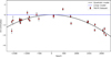 |
Fig. 1 Observed minus calculated (O − C) diagram of WASP-12b for the unpublished transits collected at Asiago (Tables 1 and 3). The reference ephemeris here is the linear part of Eq. (3), while the additional quadratic term (based on dP/dE) is plotted as a black solid line. An excess scatter in the data points with respect to the quadratic model can be seen in the figure. This is addressed in Sect. 4.4. |
Comparison of the values of period change rate and orbital decay timescale of WASP-12b as estimated by different literature works.
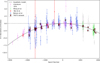 |
Fig. 2 Observed minus calculated (O − C) diagram of WASP-12b for all the available transit-timing data. The reference ephemeris here is the linear part of Eq. (4), while the additional quadratic term (based on dP/dE) is plotted as a black solid line. The Asiago data are plotted as black and red points, the remaining points come from the literature: Bai et al. (2022) (red, including TESS), Wong et al. (2022) (light green), Baluev et al. (2019) (light blue), other literature works (pink, available at CDS). Amateur timings from ETD are plotted in gray. |
4.3 The search for orbital decay in other systems
Among the population of hot Jupiters, WASP-12b is the first case where orbital decay was detected. Several studies over the years investigated the decaying orbit of hot Jupiters, which possess orbital features similar to the target of our study (Patra et al. 2020; Ivshina & Winn 2022; Hagey et al. 2022).
Harre et al. (2023) used CHEOPS and TESS high-precision photometric data to investigate the orbital decay of WASP-4b, KELT-9b and KELT-16b. In agreement with Turner et al. (2022) and Bouma et al. (2019), they found a changing orbit only for WASP-4b, but even if the orbital decay model is preferred, apsidal precession cannot be ruled out with the available data. Additional transit and occultations are needed to clearly identify the cause of the period variation.
Vissapragada et al. (2022) presented strong evidence for the tidal decay of Kepler-1658b, a close-in giant planet orbiting a subgiant star, using a 13-year observational baseline. Using RVs, the authors ruled out apsidal precession on theoretical grounds and line-of-sight acceleration. The computed value of the modified tidal quality factors  fully agrees with what should result from the dissipation of inertial waves in the convective zone. The recently discovered hot Jupiter TOI-2109b (Wong et al. 2021) presents orbital and stellar characteristics that could lead to a stronger tidal dissipation than WASP-12b. Additional new observations with a long observational baseline are needed to detect a potential orbital decay.
According to the expected tidal decay rates and host star properties, many other planets should exhibit significant rates of orbital decay, for example WASP-18b (Collier Cameron & Jardine 2018), WASP-19b (Rosário et al. 2022), WASP-43b (Patra et al. 2020), WASP-103b (Barros et al. 2022), WASP-161b (Yang & Chary 2022), KELT-16b (Harre et al. 2023) and HATS-18b (Southworth et al. 2022). To date, not enough evidence has been found from the available data to confirm a decaying orbit for any of these systems. Several effects can produce an O − C variation over a long baseline; thus, to have a successful validation of a planet tidal orbital inspiral and discard any other different possible cause a decade-long observational baseline, is necessary. Many of these targets will be reobserved by TESS, CHEOPS, PLATO (Nascimbeni et al. 2022) and Ariel (Borsato et al. 2022) in the near future and could be used in a future collective study. However, as advocated by Hamer & Schlaufman (2019), we additionally suggest that the focus of orbital decay studies should also be on planets orbiting host stars at the end of their main-sequence lifetimes.
4.4 Excess scatter in the timing data
An evident feature of our data is the presence of excess scatter in the O − C plot (Fig. 1): the reduced χ2 of the fit on the Asiago data set is  (χ2 ~ 138 for 25 d.o.f), implying that the error bars are about ~2.3 times too small with respect to a well-behaved Gaussian distribution having the same variance. This cannot be attributed to issues in the absolute calibration of our time stamps, or to systematic errors left uncorrected by our photometric pipeline, as other TASTE studies carried out with the same setup and data analysis technique demonstrated a timing accuracy at the 1 s level or better (Brown-Sevilla et al. 2021). Such an excess is not unique to our unpublished data set. The best fit to the overall O − C diagram (Fig. 2) yields
  , and other independent data sets reach a value of
  significantly larger than one (e. g.,
  for Baluev et al. 2019 and
  for ETD).
We investigated the impact of correlated noise on our results by analyzing the residuals of our light curve (i.e. after the best-fit transit model is subtracted). This was done by calculating the β factor after binning the time series on different time scales (Gillon et al. 2006; Winn et al. 2007a). When correlated noise is present, the binned rms σ is larger by a factor of β with respect to the ideal white-noise case, where the rms is supposed to decrease by the square root of the number of points per bin  . On the timescale corresponding to the ingress-egress duration (~23 min for WASP-12b), which is the most relevant timescale for the transit-time estimation, β usually lies in the 1.5–2 range for well-behaved ground-based photometry (Winn et al. 2007b). Among our 28 light curves, only four of them (#2, 7, 20, 28) show an unusually large amount of red noise (β ≫ 2), but #20 is the only one that is also a significant outlier in the O − C diagram.
As a further check, we binned each complete light curve on the timescale of the ingress duration (0.0159 days), then re-performed the global fitting process on complete transits in the same way as explained in Sect. 3.2. The resulting  is 3.2 (χ2 = 64.8 with 20 d.o.f.) which is, still considerably larger than one. Even though the error bars increased, the sign of the most significant outliers is unchanged. We also note that our best-fit dP/dt in the binned case is −29 ± 4 msec year−1, fully in agreement with the previous value of −30.7 ± 2.7 msec year−1 obtained without binning the light curves (Eq. (3)).
These exercises demonstrate that, while a few light curves show a higher-than-usual amount of correlated noise, there is no obvious link with the excess scatter we found in the measured transit times. We also note that the presence of partial transits in our data set cannot explain this excess: the reduced χ2 for just our 22 complete transits is  (χ2 = 110 for 19 d.o.f.), almost identical to the
  value for the full distribution (χ2 = 137 for 25 d.o.f.).
It is well known in the literature that comparing timing data extracted from ground-based transit light curves can be prone to systematic errors due to a combination of telluric and/or instrumental red noise and different reduction techniques (Baluev et al. 2019). On the other hand, excess scatter is sometimes noticed also when dealing with space-based data (as in Turner et al. 2022; Harre et al. 2023 in the case of WASP-4), and it is usually attributed to the presence of stellar activity. Little is known about the stellar activity properties of WASP-12b; its anomalously low RHK value could be due to the presence of extra absorption from escaped circumstellar gas (Fossati et al. 2010) and no coherent rotational modulation can be detected from its light curve. However, significant bumps are visible in the residuals of the TESS data (Wong et al. 2022), and at least one of our light curves (#23) shows an in-transit anomaly which is difficult to explain with systematic errors (Sect. 3), suggesting that in some cases inhomogeneities may arise on the stellar photosphere of WASP-12 but do not result in a detectable rotational modulation because of the high inclination of the stellar axis with respect to the observer, also suggested by the unusually low v sin i. If the poleon hypothesis is true, the timing scatter we see could be the only observable hint so far that WASP-12 is actually a significantly active star.
Intriguingly, even though running a GLS periodogram on our O − C residuals does not result in any significant frequency, the excess scatter appears to be a time-dependent phenomenon. Transits gathered during some observing seasons (such as 2011–2012 and 2019–2020) line up within seconds of the average quadratic ephemeris and return  even on the Asiago subset, while others (such as 2020-2021) appear much more scattered on different and independent data sets.
Forthcoming additional photometry from TESS (scheduled on two sectors – 71 and 72 – in November-March 2023) will possibly shed some more light on this behaviour. Meanwhile, we emphasize that, despite the scatter excess, our homogeneous data set, published here for the first time, represents a fully independent confirmation of the tidal decay process in WASP-12b, at an estimated rate perfectly consistent with those derived by previous studies.
5 Summary and conclusions
In this paper we inspected the tidal orbital decay of the ultra-hot Jupiter WASP-12b, using 28 unpublished, high-precision, ground-based light curves collected over 12 yr, from 2010 to 2022, as part of the TASTE program. We applied a DE-MCMC approach, for a linear (constant period) and quadratic model (orbital decay), to the timing of our homogeneously collected observations confirming the decaying orbit of WASP-12b.
Our new planetary and transit parameters are in good agreement with previous studies. However, combining all the timing data from literature we found some discrepancies in the O − C plot. The timing data shows an excess of scatter that cannot be attributed to errors in the photometric pipeline or the calibration of the time stamps. This raises several questions that will require further study to resolve.
We used HARPS-N observations to investigate the evolutionary stage of the host star, which is fundamental to explain the high rate of tidal dissipation. The applied spectroscopic observations allowed us to derive precise stellar parameters of the host star, however, we did not arrive at a firm conclusion regarding the evolutionary stage. The stellar parameters enable us to place the star in the main sequence close to the turn-off point and away from the subgiant branch. However, the fast tidal dissipation requires a subgiant scenario.
Acknowledgements
This publication was produced while attending the PhD program in Space Science and Technology at the University of Trento, Cycle XXXVIII, with the support of a scholarship co-financed by the Ministerial Decree no. 351 of 9th April 2022, based on the NRRP - funded by the European Union - NextGenerationEU - Mission 4 “Education and Research”, Component 2 “From Research to Business”, Investment 3.3. Based on observations collected at Copernico 1.82 m telescope and at the Schmidt 67/92 telescope. We thank the GAPS collaboration for kindly providing the spectra of WASP-12. This research has made use of the SIMBAD database (operated at CDS, Strasbourg, France;Wenger et al. 2000), the VARTOOLS Light Curve Analysis Program (version 1.39 released October 30, 2020, Hartman & Bakos 2016), TOPCAT and STILTS (Taylor 2005, 2006), NASAs Astrophysics Data System (ADS) bibliographic services. L. Bo., V. Na., and G. Pi. acknowledge support from CHEOPS ASI-INAF agreement n. 2019-29-HH.0. V.N., G.P., L.M. acknowledge financial support from the Bando Ricerca Fondamentale INAF 2023, Data Analysis Grant: “Characterization of transiting exoplanets by exploiting the unique synergy between TASTE and TESS”.
Appendix A Stacked r and R-band light curves, with the best fit-model overplotted and binned data
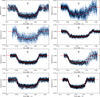 |
Fig. A.1 Individual TASTE transits light curves of WASP-12 b. The best-fitting PyORBIT model (obtained in Sect. 3.2) is shown as a red line. The ID for each transit is shown in the center of each panel. |
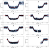 |
Fig. A.2 Same as Figure A.1 but for observations 9 through 16. |
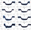 |
Fig. A.3 Same as Figure A.1 but for observations 17 through 24. |
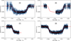 |
Fig. A.4 Same as Figure A.1 but for observations 25 through 28. |
Appendix B H-R diagram
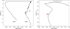 |
Fig. B.1 H-R diagram displaying the effective temperature Teff versus luminosity L/L⊙, the isochrone from the MESA Isochrone & Stellar Tracks (MIST) stellar evolution models is shown as a solid black line. The location of WASP-12 is shown with a filled blue star. The gray box marks the zoomed-in region shown in the right panel. Right: zoomed in view of the diagram. |
References
- Agol, E., Steffen, J., Sari, R., & Clarkson, W. 2005, MNRAS, 359, 567 [Google Scholar]
- Albrecht, S., Winn, J. N., Johnson, J. A., et al. 2012, ApJ, 757, 18 [NASA ADS] [CrossRef] [Google Scholar]
- Antonetti, V., & Goodman, J. 2022, ApJ, 939, 91 [CrossRef] [Google Scholar]
- Antoniciello, G., Borsato, L., Lacedelli, G., et al. 2021, MNRAS, 505, 1567 [CrossRef] [Google Scholar]
- Bai, L., Gu, S., Wang, X., et al. 2022, MNRAS, 512, 3113 [NASA ADS] [CrossRef] [Google Scholar]
- Bailey, A., & Goodman, J. 2019, MNRAS, 482, 1872 [NASA ADS] [CrossRef] [Google Scholar]
- Baluev, R. V., Sokov, E. N., Jones, H. R. A., et al. 2019, MNRAS, 490, 1294 [CrossRef] [Google Scholar]
- Barker, A. J. 2020, MNRAS, 498, 2270 [Google Scholar]
- Barros, S. C. C., Akinsanmi, B., Boué, G., et al. 2022, A&A, 657, A52 [NASA ADS] [CrossRef] [EDP Sciences] [Google Scholar]
- Batalha, N. M., Rowe, J. F., Bryson, S. T., et al. 2013, ApJS, 204, 24 [Google Scholar]
- Bell, T. J., Zhang, M., Cubillos, P. E., et al. 2019, MNRAS, 489, 1995 [Google Scholar]
- Biazzo, K., Gratton, R., Desidera, S., et al. 2015, A&A, 583, A135 [NASA ADS] [CrossRef] [EDP Sciences] [Google Scholar]
- Biazzo, K., D’Orazi, V., Desidera, S., et al. 2022, A&A, 664, A161 [NASA ADS] [CrossRef] [EDP Sciences] [Google Scholar]
- Bonomo, A. S., Desidera, S., Benatti, S., et al. 2017, A&A, 602, A107 [NASA ADS] [CrossRef] [EDP Sciences] [Google Scholar]
- Borsato, L., Nascimbeni, V., Piotto, G., & Szabó, G. 2022, Exp. Astron., 53, 635 [NASA ADS] [CrossRef] [Google Scholar]
- Bouma, L. G., Winn, J. N., Baxter, C., et al. 2019, AJ, 157, 217 [NASA ADS] [CrossRef] [Google Scholar]
- Brown-Sevilla, S. B., Nascimbeni, V., Borsato, L., et al. 2021, MNRAS, 506, 2122 [NASA ADS] [CrossRef] [Google Scholar]
- Castelli, F., & Kurucz, R. L. 2003, IAU Symp., 210, A20 [Google Scholar]
- Chakrabarty, A., & Sengupta, S. 2019, AJ, 158, 39 [NASA ADS] [CrossRef] [Google Scholar]
- Choi, J., Dotter, A., Conroy, C., et al. 2016, ApJ, 823, 102 [Google Scholar]
- Collier Cameron, A., & Jardine, M. 2018, MNRAS, 476, 2542 [Google Scholar]
- Collins, K. A., Kielkopf, J. F., & Stassun, K. G. 2017, AJ, 153, 78 [NASA ADS] [CrossRef] [Google Scholar]
- Cosentino, R., Lovis, C., Pepe, F., et al. 2012, SPIE Conf. Ser., 8446, 84461V [Google Scholar]
- Cosentino, R., Lovis, C., Pepe, F., et al. 2014, SPIE Conf. Ser., 9147, 91478C [Google Scholar]
- Covino, E., Esposito, M., Barbieri, M., et al. 2013, A&A, 554, A28 [NASA ADS] [CrossRef] [EDP Sciences] [Google Scholar]
- Cutri, R. M., Skrutskie, M. F., van Dyk, S., et al. 2003, VizieR Online Data Catalog: II/246 [Google Scholar]
- Dawson, R. I., & Johnson, J. A. 2018, ARA&A, 56, 175 [Google Scholar]
- Debrecht, A., Carroll-Nellenback, J., Frank, A., et al. 2018, MNRAS, 478, 2592 [NASA ADS] [CrossRef] [Google Scholar]
- Deheuvels, S., Brandão, I., Silva Aguirre, V., et al. 2016, A&A, 589, A93 [NASA ADS] [CrossRef] [EDP Sciences] [Google Scholar]
- Dotter, A. 2016, ApJS, 222, 8 [Google Scholar]
- Dotter, A., Chaboyer, B., Jevremovic, D., et al. 2008, ApJS, 178, 89 [NASA ADS] [CrossRef] [Google Scholar]
- Doyle, A. P., Davies, G. R., Smalley, B., Chaplin, W. J., & Elsworth, Y. 2014, MNRAS, 444, 3592 [Google Scholar]
- Dragomir, D., Kane, S. R., Pilyavsky, G., et al. 2011, AJ, 142, 115 [NASA ADS] [CrossRef] [Google Scholar]
- Dressing, C. D., & Charbonneau, D. 2013, ApJ, 767, 95 [Google Scholar]
- Eastman, J., Siverd, R., & Gaudi, B. S. 2010, PASP, 122, 935 [Google Scholar]
- Efroimsky, M., & Makarov, V. V. 2022, Universe, 8, 211 [NASA ADS] [CrossRef] [Google Scholar]
- Eggleton, P. P., Kiseleva, L. G., & Hut, P. 1998, ApJ, 499, 853 [NASA ADS] [CrossRef] [Google Scholar]
- Fabrycky, D., & Tremaine, S. 2007, ApJ, 669, 1298 [NASA ADS] [CrossRef] [Google Scholar]
- Fellay, L., Pezzotti, C., Buldgen, G., Eggenberger, P., & Bolmont, E. 2023, A&A, 669, A2 [NASA ADS] [CrossRef] [EDP Sciences] [Google Scholar]
- Feroz, F., & Hobson, M. P. 2008, MNRAS, 384, 449 [NASA ADS] [CrossRef] [Google Scholar]
- Feroz, F., Hobson, M. P., & Bridges, M. 2009, MNRAS, 398, 1601 [NASA ADS] [CrossRef] [Google Scholar]
- Feroz, F., Hobson, M. P., Cameron, E., & Pettitt, A. N. 2019, Open J. Astrophys., 2, 10 [Google Scholar]
- Foreman-Mackey, D., Hogg, D. W., Lang, D., & Goodman, J. 2013, PASP, 125, 306 [Google Scholar]
- Fortney, J. J., Dawson, R. I., & Komacek, T. D. 2021, J. Geophys. Res. Planets, 126, e06629 [NASA ADS] [CrossRef] [Google Scholar]
- Fossati, L., Haswell, C. A., Froning, C. S., et al. 2010, ApJ, 714, L222 [Google Scholar]
- Gaia Collaboration 2020, VizieR Online Data Catalog: I/350 [Google Scholar]
- Gillon, M., Pont, F., Moutou, C., et al. 2006, A&A, 459, 249 [NASA ADS] [CrossRef] [EDP Sciences] [Google Scholar]
- Goldreich, P., & Soter, S. 1966, Icarus, 5, 375 [Google Scholar]
- Granata, V., Nascimbeni, V., Piotto, G., et al. 2014, Astron. Nachr., 335, 797 [NASA ADS] [CrossRef] [Google Scholar]
- Guilluy, G., Giacobbe, P., Carleo, I., et al. 2022, A&A, 665, A104 [NASA ADS] [CrossRef] [EDP Sciences] [Google Scholar]
- Hagey, S. R., Edwards, B., & Boley, A. C. 2022, AJ, 164, 220 [NASA ADS] [CrossRef] [Google Scholar]
- Hamer, J. H., & Schlaufman, K. C. 2019, AJ, 158, 190 [Google Scholar]
- Harre, J. V., Smith, A. M. S., Barros, S. C. C., et al. 2023, A&A, 669, A124 [NASA ADS] [CrossRef] [EDP Sciences] [Google Scholar]
- Hartman, J. D., & Bakos, G. Á. 2016, Astron. Comput., 17, 1 [Google Scholar]
- Haswell, C. A., Fossati, L., Ayres, T., et al. 2012, ApJ, 760, 79 [Google Scholar]
- Hebb, L., Collier-Cameron, A., Loeillet, B., et al. 2009, ApJ, 693, 1920 [Google Scholar]
- Himes, M. D., & Harrington, J. 2022, ApJ, 931, 86 [NASA ADS] [CrossRef] [Google Scholar]
- Høg, E., Fabricius, C., Makarov, V. V., et al. 2000, A&A, 355, L27 [Google Scholar]
- Holman, M. J., & Murray, N. W. 2005, Science, 307, 1288 [Google Scholar]
- Howard, A. W., Marcy, G. W., Bryson, S. T., et al. 2012, ApJS, 201, 15 [Google Scholar]
- Hoyer, S., Pallé, E., Dragomir, D., & Murgas, F. 2016, AJ, 151, 137 [NASA ADS] [CrossRef] [Google Scholar]
- Husnoo, N., Pont, F., Mazeh, T., et al. 2012, MNRAS, 422, 3151 [NASA ADS] [CrossRef] [Google Scholar]
- Husser, T. O., Wende-von Berg, S., Dreizler, S., et al. 2013, A&A, 553, A6 [NASA ADS] [CrossRef] [EDP Sciences] [Google Scholar]
- Hut, P. 1981, A&A, 99, 126 [NASA ADS] [Google Scholar]
- Ivshina, E. S., & Winn, J. N. 2022, ApJS, 259, 62 [CrossRef] [Google Scholar]
- Jackson, B., Greenberg, R., & Barnes, R. 2008, ApJ, 678, 1396 [Google Scholar]
- Jeffries, R. D., Jackson, R. J., Wright, N. J., et al. 2023, MNRAS, 523, 802 [NASA ADS] [CrossRef] [Google Scholar]
- Kipping, D. M. 2013, MNRAS, 435, 2152 [Google Scholar]
- Kreidberg, L. 2015, PASP, 127, 1161 [Google Scholar]
- Lacedelli, G., Malavolta, L., Borsato, L., et al. 2021, MNRAS, 501, 4148 [NASA ADS] [CrossRef] [Google Scholar]
- Lai, D., Helling, C., & van den Heuvel, E. P. J. 2010, ApJ, 721, 923 [NASA ADS] [CrossRef] [Google Scholar]
- Lanza, A. F. 2020, MNRAS, 497, 3911 [NASA ADS] [CrossRef] [Google Scholar]
- Lanza, A. F., Damiani, C., & Gandolfi, D. 2011, A&A, 529, A50 [NASA ADS] [CrossRef] [EDP Sciences] [Google Scholar]
- Levrard, B., Winisdoerffer, C., & Chabrier, G. 2009, ApJ, 692, L9 [NASA ADS] [CrossRef] [Google Scholar]
- Li, S.-L., Miller, N., Lin, D. N. C., & Fortney, J. J. 2010, Nature, 463, 1054 [NASA ADS] [CrossRef] [Google Scholar]
- Lin, D. N. C., Bodenheimer, P., & Richardson, D. C. 1996, Nature, 380, 606 [Google Scholar]
- Lind, K., Asplund, M., & Barklem, P. S. 2009, A&A, 503, 541 [NASA ADS] [CrossRef] [EDP Sciences] [Google Scholar]
- Maciejewski, G., Errmann, R., Raetz, S., et al. 2011, A&A, 528, A65 [NASA ADS] [CrossRef] [EDP Sciences] [Google Scholar]
- Maciejewski, G., Dimitrov, D., Fernández, M., et al. 2016, A&A, 588, L6 [NASA ADS] [CrossRef] [EDP Sciences] [Google Scholar]
- Maciejewski, G., Fernandez, M., Aceituno, F., et al. 2018, Acta Astron., 68, 371 [NASA ADS] [Google Scholar]
- Malavolta, L., Nascimbeni, V., Piotto, G., et al. 2016, A&A, 588, A118 [NASA ADS] [CrossRef] [EDP Sciences] [Google Scholar]
- Malavolta, L., Mayo, A. W., Louden, T., et al. 2018, AJ, 155, 107 [NASA ADS] [CrossRef] [Google Scholar]
- Mallonn, M., von Essen, C., Herrero, E., et al. 2019, A&A, 622, A81 [EDP Sciences] [Google Scholar]
- Matsumura, S., Peale, S. J., & Rasio, F. A. 2010, ApJ, 725, 1995 [Google Scholar]
- Meibom, S., & Mathieu, R. D. 2005, ApJ, 620, 970 [Google Scholar]
- Meibom, S., Barnes, S. A., Platais, I., et al. 2015, Nature, 517, 589 [Google Scholar]
- Millholland, S., & Laughlin, G. 2018, ApJ, 869, L15 [CrossRef] [Google Scholar]
- Miralda-Escudé, J. 2002, ApJ, 564, 1019 [Google Scholar]
- Morton, T. D. 2015, Astrophysics Source Code Library [record ascl:1503.010] [Google Scholar]
- Nagasawa, M., Ida, S., & Bessho, T. 2008, ApJ, 678, 498 [NASA ADS] [CrossRef] [Google Scholar]
- Nascimbeni, V., Piotto, G., Bedin, L. R., & Damasso, M. 2011, A&A, 527, A85 [NASA ADS] [CrossRef] [EDP Sciences] [Google Scholar]
- Nascimbeni, V., Cunial, A., Murabito, S., et al. 2013, A&A, 549, A30 [NASA ADS] [CrossRef] [EDP Sciences] [Google Scholar]
- Nascimbeni, V., Piotto, G., Börner, A., et al. 2022, A&A, 658, A31 [NASA ADS] [CrossRef] [EDP Sciences] [Google Scholar]
- Nelson, R. P., Papaloizou, J. C. B., Masset, F., & Kley, W. 2000, MNRAS, 318, 18 [NASA ADS] [CrossRef] [Google Scholar]
- Nichols, J. D., Wynn, G. A., Goad, M., et al. 2015, ApJ, 803, 9 [NASA ADS] [CrossRef] [Google Scholar]
- Ogilvie, G. I., & Lin, D. N. C. 2007, ApJ, 661, 1180 [Google Scholar]
- Parmentier, V., Line, M. R., Bean, J. L., et al. 2018, A&A, 617, A110 [NASA ADS] [CrossRef] [EDP Sciences] [Google Scholar]
- Patra, K. C., Winn, J. N., Holman, M. J., et al. 2017, AJ, 154, 4 [Google Scholar]
- Patra, K. C., Winn, J. N., Holman, M. J., et al. 2020, AJ, 159, 150 [NASA ADS] [CrossRef] [Google Scholar]
- Paxton, B., Bildsten, L., Dotter, A., et al. 2011, ApJS, 192, 3 [Google Scholar]
- Penev, K., Bouma, L. G., Winn, J. N., & Hartman, J. D. 2018, AJ, 155, 165 [NASA ADS] [CrossRef] [Google Scholar]
- Poddaný, S., Brát, L., & Pejcha, O. 2010, New A, 15, 297 [CrossRef] [Google Scholar]
- Rasio, F. A., Tout, C. A., Lubow, S. H., & Livio, M. 1996, ApJ, 470, 1187 [Google Scholar]
- Rosário, N. M., Barros, S. C. C., Demangeon, O. D. S., & Santos, N. C. 2022, A&A, 668, A114 [NASA ADS] [CrossRef] [EDP Sciences] [Google Scholar]
- Sasselov, D. D. 2003, ApJ, 596, 1327 [NASA ADS] [CrossRef] [Google Scholar]
- Schwarz, G. 1978, Annal. Stat., 6, 461 [Google Scholar]
- Sestito, P., & Randich, S. 2005, A&A, 442, 615 [NASA ADS] [CrossRef] [EDP Sciences] [Google Scholar]
- Silburt, A., Gaidos, E., & Wu, Y. 2015, ApJ, 799, 180 [Google Scholar]
- Skrutskie, M. F., Cutri, R. M., Stiening, R., et al. 2006, AJ, 131, 1163 [NASA ADS] [CrossRef] [Google Scholar]
- Sneden, C. 1973, AJ, 184, 839 [NASA ADS] [CrossRef] [Google Scholar]
- Southworth, J., Barker, A. J., Hinse, T. C., et al. 2022, MNRAS, 515, 3212 [NASA ADS] [CrossRef] [Google Scholar]
- Stangret, M., Casasayas-Barris, N., Pallé, E., et al. 2022, A&A, 662, A101 [NASA ADS] [CrossRef] [EDP Sciences] [Google Scholar]
- Taylor, M. B. 2005, ASP Conf. Ser., 347, 29 [Google Scholar]
- Taylor, M. B. 2006, ASP Conf. Ser., 351, 666 [Google Scholar]
- Turner, J. D., Ridden-Harper, A., & Jayawardhana, R. 2021, AJ, 161, 72 [NASA ADS] [CrossRef] [Google Scholar]
- Turner, J. D., Flagg, L., Ridden-Harper, A., & Jayawardhana, R. 2022, AJ, 163, 281 [NASA ADS] [CrossRef] [Google Scholar]
- Vissapragada, S., Chontos, A., Greklek-McKeon, M., et al. 2022, ApJ, 941, L31 [NASA ADS] [CrossRef] [Google Scholar]
- Weinberg, N. N., Sun, M., Arras, P., & Essick, R. 2017, ApJ, 849, L11 [Google Scholar]
- Weinberg, N. N., Davachi, N., Essick, R., et al. 2024, ApJ, 960, 50 [NASA ADS] [CrossRef] [Google Scholar]
- Wenger, M., Ochsenbein, F., Egret, D., et al. 2000, A&AS, 143, 9 [NASA ADS] [CrossRef] [EDP Sciences] [Google Scholar]
- Winn, J. N. 2010, in Exoplanets, ed. S. Seager (Tucson: University of Arizona Press), 55 [Google Scholar]
- Winn, J. N., Holman, M. J., Bakos, G. Á., et al. 2007a, AJ, 134, 1707 [NASA ADS] [CrossRef] [Google Scholar]
- Winn, J. N., Holman, M. J., Henry, G. W., et al. 2007b, AJ, 133, 1828 [NASA ADS] [CrossRef] [Google Scholar]
- Wong, I., Shporer, A., Zhou, G., et al. 2021, AJ, 162, 256 [NASA ADS] [CrossRef] [Google Scholar]
- Wong, I., Shporer, A., Vissapragada, S., et al. 2022, AJ, 163, 175 [NASA ADS] [CrossRef] [Google Scholar]
- Wright, E. L., Eisenhardt, P. R. M., Mainzer, A. K., et al. 2010, AJ, 140, 1868 [Google Scholar]
- Wu, Y., & Lithwick, Y. 2011, ApJ, 735, 109 [Google Scholar]
- Yang, F., & Chary, R.-R. 2022, AJ, 164, 259 [CrossRef] [Google Scholar]
- Yee, S. W., Winn, J. N., Knutson, H. A., et al. 2020, ApJ, 888, L5 [Google Scholar]
- Zahn, J. P. 1977, A&A, 57, 383 [Google Scholar]
- Zahn, J. P. 2008, EAS Pub. Ser., 29, 67 [NASA ADS] [CrossRef] [EDP Sciences] [Google Scholar]
All Tables
WASP-12b orbital parameters derived from PyORBIT Markov chain Monte Carlo analysis.
Stellar parameters of WASP-12 derived from the analysis of the HARPS-N spectra and from stellar evolutionary tracks.
Comparison of the values of period change rate and orbital decay timescale of WASP-12b as estimated by different literature works.
All Figures
|
Fig. 1 Observed minus calculated (O − C) diagram of WASP-12b for the unpublished transits collected at Asiago (Tables 1 and 3). The reference ephemeris here is the linear part of Eq. (3), while the additional quadratic term (based on dP/dE) is plotted as a black solid line. An excess scatter in the data points with respect to the quadratic model can be seen in the figure. This is addressed in Sect. 4.4. |
| In the text | |
|
Fig. 2 Observed minus calculated (O − C) diagram of WASP-12b for all the available transit-timing data. The reference ephemeris here is the linear part of Eq. (4), while the additional quadratic term (based on dP/dE) is plotted as a black solid line. The Asiago data are plotted as black and red points, the remaining points come from the literature: Bai et al. (2022) (red, including TESS), Wong et al. (2022) (light green), Baluev et al. (2019) (light blue), other literature works (pink, available at CDS). Amateur timings from ETD are plotted in gray. |
| In the text | |
|
Fig. A.1 Individual TASTE transits light curves of WASP-12 b. The best-fitting PyORBIT model (obtained in Sect. 3.2) is shown as a red line. The ID for each transit is shown in the center of each panel. |
| In the text | |
|
Fig. A.2 Same as Figure A.1 but for observations 9 through 16. |
| In the text | |
|
Fig. A.3 Same as Figure A.1 but for observations 17 through 24. |
| In the text | |
|
Fig. A.4 Same as Figure A.1 but for observations 25 through 28. |
| In the text | |
|
Fig. B.1 H-R diagram displaying the effective temperature Teff versus luminosity L/L⊙, the isochrone from the MESA Isochrone & Stellar Tracks (MIST) stellar evolution models is shown as a solid black line. The location of WASP-12 is shown with a filled blue star. The gray box marks the zoomed-in region shown in the right panel. Right: zoomed in view of the diagram. |
| In the text | |
Current usage metrics show cumulative count of Article Views (full-text article views including HTML views, PDF and ePub downloads, according to the available data) and Abstracts Views on Vision4Press platform.
Data correspond to usage on the plateform after 2015. The current usage metrics is available 48-96 hours after online publication and is updated daily on week days.
Initial download of the metrics may take a while.