| Issue |
A&A
Volume 668, December 2022
|
|
|---|---|---|
| Article Number | A114 | |
| Number of page(s) | 15 | |
| Section | Planets and planetary systems | |
| DOI | https://doi.org/10.1051/0004-6361/202244513 | |
| Published online | 13 December 2022 | |
Measuring the orbit shrinkage rate of hot Jupiters due to tides
1
Instituto de Astrofísica e Ciências do Espaço, CAUP, Rua das Estrelas,
4150-762
Porto, Portugal
e-mail: This email address is being protected from spambots. You need JavaScript enabled to view it.
2
Departamento de Fisica e Astronomia, Faculdade de Ciências, Universidade do Porto,
Rua do Campo Alegre 687,
4169-007
Porto, Portugal
Received:
15
July
2022
Accepted:
16
October
2022
Abstract
Context. A tidal interaction between a star and a close-in exoplanet leads to shrinkage of the planetary orbit and eventual tidal dis- ruption of the planet. Measuring the shrinkage of the orbits will allow for the tidal quality parameter of the star (Q★′) to be measured, which is an important parameter to obtain information about stellar interiors.
Aims. We analyse data from the Transiting Exoplanet Survey Satellite (TESS) for two targets known to host close-in hot Jupiters, which have significant data available and are expected to have a fast decay: WASP-18 and WASP-19. We aim to measure the current limits on orbital period variation and provide new constrains on Q★′ for our targets.
Methods. We modelled the transit shape using all the available TESS observations and fitted the individual transit times of each tran- sit. We used previously published transit times together with our results to fit two models, a constant period model, and a quadratic orbital decay model, using Markov chain Monte Carlo (MCMC) algorithms.
Results. We obtain new constrains on Q★′ for both targets and improve the precision of the known planet parameters with the newest observations from TESS. We find period change rates of (−0.11 ± 0.21) × 10−10 for WASP-18b and (−0.35 ± 0.22) × 10−10 for WASP-19b and we do not find significant evidence of orbital decay in these targets. We obtain new lower limits for Q★′ of (1.42 ± 0.34) × 107 in WASP-18 and (1.26 ± 0.10) × 106 in WASP-19, corresponding to upper limits of the orbital decay rate of −0.45 × 10⁻¹⁰ and −0.71 × 10⁻¹⁰, respectively, with a 95% confidence level. We compare our results with other relevant targets for tidal decay studies.
Conclusions. We find that the orbital decay rate in both WASP-18b and WASP-19b appears to be smaller than the measured orbital decay of WASP-12b. We show that the minimum value of Q★′ in WASP-18 is two orders of magnitude higher than that of WASP-12, while WASP-19 has a minimum value one order of magnitude higher, which is consistent with other similar targets. Further observations are required to constrain the orbital decay of WASP-18 and WASP-19.
Key words: planets and satellites: fundamental parameters / planets and satellites: dynamical evolution and stability / techniques: photometric / planet-star interactions
© N. M. Rosário et al. 2022
 Open Access article, published by EDP Sciences, under the terms of the Creative Commons Attribution License (https://creativecommons.org/licenses/by/4.0), which permits unrestricted use, distribution, and reproduction in any medium, provided the original work is properly cited.
This article is published in open access under the Subscribe-to-Open model. This email address is being protected from spambots. You need JavaScript enabled to view it. to support open access publication.
1 Introduction
In 1995, 51 Pegasi b became the first exoplanet discovered orbit- ing a solar-like star (Mayor & Queloz 1995). It is a massive planet, about half the mass of Jupiter, with a short period, orbit- ing close to its host star. These planets, now known as hot Jupiters due to their size and high temperature, have been found around several systems and provide an astronomical laboratory for our physical models of planetary formation and evolution, as well as planet-star interaction. Hot Jupiters are an uncommon presence around Sun-like stars when compared to smaller plan- ets (Howard et al. 2012; Wright et al. 2012; Johnson et al. 2010), and the circumstances of their formation and evolution are still not completely understood (e.g. Dawson & Johnson 2018). Due to their size and short period, these planets have a high signal-to-noise ratio (S/N), making it easier to obtain data on them and turning hot Jupiters into an important source of information regarding the physics of planet formation and evolution.
Due to the proximity to their host star, hot Jupiters are strongly affected by tidal forces. In cases where the rotation of the star is not synchronised with the orbital period of the planet, a transfer of angular moment occurs, leading to an increase in the rotation of the star and a shrinkage of the planet’s orbit. This effect, known as tidal decay (Counselman III 1973; Levrard et al. 2009; Matsumura et al. 2010), gives important information about the tidal interaction between a planet and star and helps to con- strain stellar physics through the tidal quality factor  . This parameter measures the efficiency of the energy dissipation dur- ing tidal interactions and is related to the propagation of tidal oscillations inside the star (Ogilvie & Lin 2007; Ogilvie 2014). According to the theory developed by Zahn (1975, 1977), larger stars with convective cores and radiative envelopes are expected to have a less efficient dissipation and, therefore, a larger value of
  .
.
Other physical processes can, in the short term, result in a shift in period that is similar to tidal decay: apsidal precession (Miralda-Escudé 2002; Heyl & Gladman 2007; Jordán & Bakos 2008; Ragozzine & Wolf 2009) and the presence of external bodies affecting their orbits (Gibson et al. 2009, 2010). Apsidal precession is the rotation of the ascending node along the orbital plane and as such, this effect is periodic and does not lead to a long-term decay of the orbit. Additionally, a change in period may arise from gravitational effects from nearby compan- ions disturbing the orbit. An example of this effect is reported by Triaud et al. (2017) in their study of the system architecture of WASP-53 and WASP-81. Turner et al. (2021a) have recently sug- gested that the orbit of WASP-4b (Wilson et al. 2008) may also be changing because of another companion nearby.
WASP-12b, a hot Jupiter orbiting a late F-type star, was the first target confirmed as having a decaying orbit caused by tidal interactions (Patra et al. 2017; Maciejewski et al. 2018; Turner et al. 2021b; Wong et al. 2022). It orbits its star with a period of 1.09 days, and has a mass of 1.5 MJ and a radius of 1.90 RJ. Its orbit is shrinking at a rate of 29.81 ± 0.94 m s yr−1, leading to a decay timescale of 3.16 ± 0.10 Myr. The tidal quality factor of  is thought to be on the lower side of the predicted values (Wong et al. 2022).
Despite being one of the prime targets to measure tidal decay (Patra et al. 2020), so far there is still no evidence towards a decaying period in WASP-18b, with Maciejewski et al. (2020) placing a lower limit for  of 3.9 × 10⁶ at 95% confidence level. The value is of the same order of magnitude as the ones found by Shporer et al. (2019) and Patra et al. (2020), which also investigated this system. WASP-19b (Hebb et al. 2009), which is one of the shortest period hot Jupiters reported to date (0.78 days), is also an interesting target for tidal decay stud- ies. Several authors have studied this system (e.g. Hellier et al. 2009; Tregloan-Reed et al. 2013; Espinoza et al. 2019; Petrucci et al. 2020) and Patra et al. (2020) found statistically signifi- cant evidence towards a decreasing period, with Ṗ = dP/dt = (−2.06 ± 0.42) × 10−10. However, WASP-19 is a highly active star, leading to distortions in the light curves thought to be caused by star spots (Tregloan-Reed et al. 2013; Espinoza et al. 2019). The result by Petrucci et al. (2020), discarding tidal decay in WASP-19, contradicts these previous results, finding a value of Ṗ = 0.0114 ± 0.74 × 10⁻¹⁰ consistent with zero, and increases the importance of continuing observations of this system.
In this paper, we present our analysis of the Transiting Exoplanet Survey Satellite (TESS; Ricker et al. 2014) data concern- ing two hot Jupiters expected to show orbital decay, WASP-18b and WASP-19b. We aim to search for signs of tidal decay on these targets and to measure the current constrains on the tidal decay parameters, which allow us to better understand the migra- tion mechanisms of hot Jupiters and the reasons behind the decaying orbits.
We describe our target systems and the process of target selection in Sect. 2. In Sect. 3, we present the TESS data and the pre-processing of the light curves. The transit analysis is listed in Sect. 4 and in Sect. 5 we describe our transit timing variation (TTV) and orbital decay models. We present and dis- cuss the results of the TTV analysis in Sect. 6 and provide a short summary of the current status of orbital decay studies in other systems in Sect. 7. Finally, a summary and conclusion is presented in Sect. 8.
2 Target selection
In order to work with the most relevant targets we looked at several hot Jupiters that orbit close to their stars. We mainly focussed on the expected orbital decay rate of those planets in order to explore the most promising candidates. Patra et al. (2020) plotted the scaled orbital semi-major axis a/R★ against the planet-to-star mass ratio Mp/M★, two quantities that are pro- portional to the decay rate according to the current orbital decay models, and they provided several cutoffs based on the decay rate for a constant  in a population of cold and hot stars brighter than V = 14.5. We followed the approach taken in that paper and started by looking at a sample of 12 targets, six candidates orbit- ing hot stars (Teff > 6000 K) and six orbiting cold stars, with an expected decay rate of dP/dT < 107 yr for a
  .
.
We then looked at the targets that have been observed by TESS in more than one season and whose data were not already published, so as to be able to obtain the maximum amount of transits and therefore obtain the best possible constrain on the orbital decay parameters. We also looked at the previous avail- able data from other observations to ensure the data span a large enough timescale to possibly detect a change in period. For example, HATS-18 (Penev et al. 2016) would seem promis- ing with the previous criteria; however, the lack of previous data makes it hard, if not impossible, to properly search for period changes. WASP-4 (Wilson et al. 2008) and WASP-43 (Hellier et al. 2011), for example, would also make for good targets in this study; however, orbital decay analyses using the available data from TESS were recently published (WASP-4: Turner et al. 2021a; WASP-43: Davoudi et al. 2021).
According to Patra et al. (2020), it is expected that planets around colder stars have a faster tidal dissipation due to their larger convective envelopes. Therefore, it can be important to investigate tidal decay around both hot and cold stars. Given the previous criteria and taking stellar temperature into account, we looked into the best candidates orbiting a hot star and the best candidates orbiting a cold star. From the original sample, WASP-18 is shown to be one of the most promising candidates for tidal decay thanks to its high Mp/M★ ratio. Furthermore, it was observed by TESS in a total of four sectors, which gives us a good amount of data to work with, and it has been the subject of several decay studies and previous observations (e.g. Shporer et al. 2019; Maciejewski et al. 2020). WASP-19 is one of the most promising targets among cold stars. It has avail- able data from TESS in two sectors and has been studied for several years (e.g. Mancini et al. 2013; Espinoza et al. 2019), with observations from different instruments in both photometry and spectroscopy, in part due to the high stellar activity that is present in the star. The additional TESS data may also provide new input to understand the effect of the activity in the orbital decay studies.
2.1 WASP-18
WASP-18b (Hellier et al. 2009; Southworth et al. 2009) is a mas- sive hot Jupiter with a mass of 11.4 MJ and a radius of 1.20 RJ, orbiting its star on a period of 0.94 days. The star, WASP-18, is a bright (V = 9.30) F-type star with a mass of 1.46 M⊙, an effec- tive temperature of 6431 K, and an estimated age of 1 Gyr (Patra et al. 2020). Several authors have looked at this system before to try to find evidence of tidal decay since, according to theoretical models, WASP-18b should be one of the fastest decaying targets we know of, in part due to its large mass relative to the star. How- ever, Wilkins et al. (2017) initially found no evidence of rapid decay. McDonald & Kerins (2018) included an early transit for HIPPARCOS and found a weak sign of decay, but one must take the high uncertainty in the timing of the HIPPARCOS transit into account. With the first TESS observations for WASP-18, in Sectors 2 and 3, new constrains have been found in the tidal decay parameters, with Shporer et al. (2019) and Maciejewski et al. (2020) reporting results consistent with the findings of Wilkins et al. (2017), with the new data not showing enough evi- dence to confirm the decay of the orbit of WASP-18b. With two additional TESS sectors and a 2-yr gap between observations, we expect to add an additional constraint to the tidal decay parame- ters and strengthen the evidence towards the presence or absence of rapid decay.
2.2 WASP-19
WASP-19b (Hebb et al. 2009) is a Jupiter-sized planet with 1.14 MJ and 1.4 RJ orbiting an active solar-type G-star with around 10 Gyr, a mass of 0.9 M⊙, and an effective temperature of 5460 K. It is one of the shortest-period hot Jupiters discovered so far, with a period of 0.78 days, and it was surpassed recently by the discovery of TOI-2109 with a period of 0.67 days (Wong et al. 2021). With the high amount of activity reported, WASP-19 is an interesting but challenging target to measure orbital decay. Several authors have obtained WASP-19b transits (e.g. Mancini et al. 2013; Espinoza et al. 2019), and Patra et al. (2020) added their own transits to previous data and found strong evidence of decay, with a period change rate of −6.50 ± 1.33 ms yr−1. How- ever, they suspect stellar activity is causing systematic errors and the result may be misleading. This evidence is further weak- ened by Petrucci et al. (2020), who include several more recent transits from the literature and from their own observations and show evidence towards a constant period, with a value of Ṗ = 0.015 ± 0.96 m s yr−1 consistent with zero. Despite this, they pro- vide an upper limit for Ṗ of −2.294 m s yr−1. The newest TESS observations might shed some new light on WASP-19b and the true nature of its orbital period and help to clarify the behaviour of this hot Jupiter.
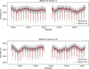 |
Fig. 1 PDC light curves of WASP-19 with NaNs and quality flagged points removed. Moving median filter over 32 points shown in red. Long-term trends can be observed in both sectors, most likely due to stellar activity or uncorrected systematic errors. |
3 TESS data
3.1 Observations
WASP-18 (TIC 100100827) was observed by Camera 2 of TESS with a 2 min cadence in Sector 2 (from 2018 August 22 to 2018 September 20), Sector 3 (from 2018 September 20 to 2018 October 18), Sector 29 (from 2020 August 26 to 2020 Septem- ber 21), and Sector 30 (from 2020 September 23 to 2020 October 20). A total of 92 transits were extracted from the observations.
WASP-19 (TIC 35516889) was observed with the same cadence by Camera 2 of TESS in Sector 9 (from 2019 February 28 to 2019 March 26) and Sector 36 (from 2021 March 07 to 2021 April 01). We extracted 56 transits from the observations.
The TESS light curves were downloaded through the Mikulski Archive for Space Telescopes (MAST) portal1. For the analysis performed in this work, we use the Presearch Data Conditioning Simple Aperture Photometry (PDCSAP) curves, which remove long-term non-astrophysical trends from the data and reduce systematic errors (Smith et al. 2012, 2017).
The data files include a quality parameter that indicates data points that have been affected by anomalous events such as atti- tude tweaks, momentum dumps, firing of thrusters, and other events (Tenenbaum & Jenkins 2018). We removed all non-zero quality flagged data points from our light curve to ensure reliable data and removed all NaN values caused by poor instrumental behaviour, but long-term trends are still present in the initial curves, especially in WASP-19 (Fig. 1). This may be caused by the high stellar activity of WASP-19 (Hebb et al. 2009; Espinoza et al. 2019; Wong et al. 2020), as well as some uncorrected systematic trends, and additional corrections are described in Sect. 3.2.
Some incomplete transits are seen in Figs. 1 and 2, espe- cially near the gaps in the middle which separate the two physical orbits from TESS. During the light curve processing described in Sect. 3.2, these incomplete transits were discarded, since the lack of a complete transit does not allow for a precise derivation of the transit timing (Barros et al. 2013).
 |
Fig. 2 PDC light curves of WASP-18 with NaNs and quality flagged points removed. Moving median filter over 32 points shown in red. Incomplete transits are shown near the gaps that separate the two physical orbits of the spacecraft. |
3.2 Stellar activity correction
As mentioned before, stellar activity is a likely cause of the trends shown in WASP-19 data (Fig. 1). To take the effect of stellar activity and spots into account, we assume the maximum flux to correspond to the minimum amount of stellar spots. We applied a moving median filter over 32 points to each light curve and found the maximum median flux over all light curves in each target. We then used this value as the normalisation constant to obtain the relative flux. We also considered the maximum of each sector light curve for normalisation instead of the overall maxi- mum, but the difference in the final result was not significant and we decided to keep the original approach. It is, however, impor- tant to note that this does not correct for spot occultation events (e.g. Barros et al. 2013).
The normalised curve was then split into individual transits. For that, we started by flagging the data points within three tran- sit durations of the mid-transit time and by splitting the light curves into individual segments, removing the remaining data between transits, which allowed for an easier capture of short-term trends near the transits while minimising the influence of long-term trends. We applied a detrending model using a low-order polynomial and used the Bayesian information criterion (BIC) to find the optimal polynomial order for each segment. The vast majority of the individual light curves favoured a first-order polynomial trend, with only a few exceptions in WASP-18 favouring a second-order model. We normalised each individual transit light curve to an out of transit level of1 using the obtained best-fit coefficients.
4 Transit analysis
The transits were modelled using the model from batman (Kreidberg 2015) and we split our analysis into two parts. First we performed a fit of all transits aiming to obtain the tran- sit parameters. We put together all individual segments already detrended and fit for reference time T0, period P, planet-to-star radius ratio rp/R★, scaled orbital semi-major axis a/R★, orbital inclination i, and the two limb-darkening coefficients of the quadratic model u1 and u2. Circular orbits with fixed e = 0 and ω = 90° were used in all analyses. The circularisation timescale for WASP-18b is around 15Myr, while WASP-19b has a value around 2 Myr; both are at least an order of magnitude lower than the estimated system ages. Because of this, we expect the eccentricity to be zero in both planets, unless external perturba- tions occur. Nevertheless, we also fitted a model with varying eccentricity using Gaussian priors, and compared the fits using the BIC. We found that the circular models were strongly pre- ferred (with a lower BIC) over the eccentric models. Therefore, we assumed a circular model for all the remaining analyses in this paper.
We used a quadratic limb-darkening model with values esti- mated with the Limb-Darkening Toolkit (LDTk, Parviainen & Aigrain 2015) using the effective temperature (Teff), gravity (log g), and metallicity ([Fe/H]) of each star. The stellar param- eters as well as the initial limb-darkening values can be found in Table 1.
We used a Markov chain Monte Carlo (MCMC) algo- rithm based on the emcee ensemble sampler in Python (Foreman-Mackey et al. 2013) for the transit analysis. We defined a number of walkers of 4 times the number of fitted parame- ters over 10 000 steps and discarded the burn-in before retrieving the results from the posterior distributions. We defined uniform priors for all parameters except the limb-darkening coefficients, for which we defined Gaussian priors centred in the values from LDTk with a conservative standard deviation of 0.1. The results of the transit analysis and the best-fit parameters are plotted in Figs. 3 and 4 and listed in Table 2 together with the used pri- ors. We obtained updated planetary and transit parameters for both targets with good agreement with the parameters obtained previously.
For the second part of the analysis, we fitted the mid-transit times of each transit separately. We fixed the previously obtained value for P, u1, and u2, allowing rp/R★, a/R★, and i to float with Gaussian priors defined by the posteriors from the previous anal- ysis. A uniform prior was used for the mid-transit time Tmid. We used the same MCMC approach as for the first part of the analy- sis, with a number of walkers equal to 4 times the number of free parameters over 5000 steps for each transit, discarding burn-in, and included a first-degree polynomial trend in the fit to propa- gate detrending errors in all curves. In this analysis, we obtained precise timings for all TESS transits currently available, which are listed in Tables A.1 and A.2 together with previously obtained transits and their origin paper.
Sectors 2 and 3 of WASP-18 have been analysed previously by Shporer et al. (2019) and Maciejewski et al. (2020). Our results agree with the ones from Maciejewski et al. (2020) within 0.5−1σ for the period and radius and 2σ for a/R★ and incli- nation. Shporer et al. (2019) considered a non-zero eccentricity for their analysis and did not fit the limb-darkening parameters, which leads to a more significant deviation from our results, with a 3σ agreement in radius but a deviation of 2–3% in a/R★ and inclination.
The radius of WASP-19b significantly deviates from previ- ous works. Espinoza et al. (2019) compare their results with the ones from Hebb et al. (2009), Tregloan-Reed et al. (2013), and Mancini et al. (2013) with good agreement; however, Wong et al. (2020) used sector 9 of TESS and found an increase of 10- 15% in the transit depth, reporting a value of 23 240 ppm against 20 258 ppm as reported by Espinoza et al. (2019). We ran individ- ual fits of sectors 9 and 36 and found that between both sectors there is a significant difference of around 3% in depth, with 21590 ppm in sector 9 and 20 996 ppm in sector 36. While our transit depth estimation is not as far from the previous ones as the one from Wong et al. (2020), we still find an increase of over 4% in depth comparing our value with Espinoza et al. (2019) using both TESS sectors (21 145 ppm), and over 6% if we use sector 9 only. Wong et al. (2020) suggest that an increase in stellar spots on the surface during sector 9 measurements is the cause for the apparently bigger radius. Our smaller difference when only using sector 9 data may therefore arise from our initial correction with individual transit segments and posterior normalisation, which was aimed to minimise the effect of spots. The different values obtained for sector 36 and the fact that the remaining parameters all agree with Espinoza et al. (2019) in <1σ levels suggests stel- lar activity is indeed high and is causing significant variations in the transit depths when using TESS data.
System stellar parameters for each target, with WASP-18 parameters obtained from Shporer et al. (2019) and WASP-19 param- eters obtained from Mancini et al. (2013).
 |
Fig. 3 Best-fit model for WASP-18b phase-folded light curve of all TESS transits. |
 |
Fig. 4 Best-fit model for WASP-19b phase-folded light curve of all TESS transits. |
System parameters and priors used in the transit modelling.
5 Timing and orbital decay analysis
The main goal of our paper is to better constrain tidal decay in promising targets. We used our derived transit times from TESS together with other transit times from the literature to look for TTVs in WASP-18b and WASP-19b. All timings are listed in Tables A.1 and A.2, referencing the original paper where the transit was first reported. However, Maciejewski et al. (2020), while compiling all previous transits of WASP-18b, ran new photometric analyses of the majority of the reported transits. Several transits from TRESCA used by Petrucci et al. (2020) were excluded from the WASP-19 TTV analysis. While they correspond to recent observations, we verified the normalised residuals of those times against a constant period model and found a high amount of scatter and high uncertainties when com- pared to TESS transits. Since the data are contemporary with the more precise TESS transits, we decided not to include them in the analysis.
In order to study the period variations in both targets, we estimated the time of each individual transit as a function of the epoch using a linear and a quadratic model. The linear model assumes a circular orbit with a constant period as
 (1)
(1)
where T0 is the reference mid-transit time (E = 0), P is the orbital period, and E is the epoch number counted from T0. The quadratic model includes an additional term, taking a uniform period change into account as
 (2)
(2)
where Ṗ = dP/dT is the rate of change in orbital period given by its derivative over time.
Comparing the two models using the BIC allowed us to look for a significant detection of a period change. The derivative over time is related to the star tidal quality factor Q★, which corre- sponds to the rate of energy dissipation due to tidal interactions (Goldreich & Soter 1966). The larger the value of Q★, the lower the tidal dissipation efficiency is. We used a parametrisation for Q★ from the tidal interaction model by Zahn (1977)
 (3)
(3)
where k★ is the stellar Love number, which measures how much of the star’s density is concentrated in its core and is related to its response to tidal forces. This leads to a relationship between  and Ṗ
and Ṗ
 (4)
(4)
Where Mp/M★ is the planet-star mass ratio and a/R★ is the scaled orbital semi-major axis. Planets similar to WASP-18b, with a high planet-star mass ratio, are very good candidates for tidal decay studies.
We assumed Gaussian priors for T0 and P, using the pre- vious best-fit values and uncertainties, and a uniform prior for Ṗ, u(−10, 2). We ran an MCMC analysis with the emcee code using all available transit times Tmid to fit for the value of Ṗ and refine T0 and P. We ran the model over 32 walkers with 10 000 steps each, discarding burn-in.
Best-fit results for our TTV analysis, with the linear constant period model and the quadratic model of orbital decay.
6 Results and discussion
The results for the TTV fits are listed in Table 3. We compared the BIC values of the linear and quadratic models, with the lin- ear model being favoured for both targets (−4.09 against 0.73 for WASP-18b and −3.91 against 0.85 for WASP-19b), suggesting there is still no significant evidence towards a change in orbital period. The best-fit quadratic models are plotted in Figs. 5 and 6.
We see from Table 3 and Fig. 7 that the Ṗ value for WASP-18b is still far from showing evidence of decay, being comfortably compatible with zero at 1σ and thus favouring a constant period. The most recent studies of WASP-18b by Shporer et al. (2019), Maciejewski et al. (2020), and Patra et al. (2020) report values consistent with these findings, with the ones of the latter being the closest to a varying period with Ṗ = (−1.2 ± 1.3) × 10−10. WASP-18b has a relatively high planet- star mass ratio, which makes it one of the main targets for observing tidal decay. Wilkins et al. (2017) estimated a minimum of  > 106 at 95% confidence; this value was only slightly improved by Shporer et al. (2019) and Maciejewski et al. (2020) using TESS data (see Table 4). We are able to improve upon the minimum value of
  with the additional transits from Sec- tors 29 and 30 by an order of magnitude compared to previous works. Despite the increased precision, we did not detect evi- dence of tidal decay in the orbit of WASP-18b and so we derived a lower limit of
  > (1.42 ± 0.34) × 107 at 95% confidence, corresponding to a Ṗ upper limit of −0.45 × 10⁻¹⁰. From our result of
  , the estimated spiral in-fall timescale is around 5 × 10⁷ yr, which is longer than originally expected. For compari- son, WASP-12b, the only planet with confirmed tidal decay so far has a corresponding
  = (1.50 ± 0.11) × 105 (Wong et al. 2022), which is two orders of magnitude lower than the minimum value we found for WASP-18. WASP-12 is also an F-type star, with an effective temperature of 6150 K, with a mass similar to WASP-18. If we assume Eq. (4) to be correct and
  to be the same for the same type of stars, WASP-18b should have a faster decay than WASP-12b, due to the planet-star mass ratio (which is 10 times higher). The absence of significant decay in WASP-18b so far shows that despite the similar stellar type and mass,
  is significantly different between the systems, suggesting the tidal dissipation processes may differ within stars of a similar type.
WASP-19b shows a decay rate different from zero at a 1σ level (Table 3 and Fig. 7). Comparing our results with the ones obtained by Patra et al. (2020), our value of  is higher than theirs by almost an order of magnitude, with our Ṗ absolute value being almost 6 times smaller, deviating from theirs by more than 7σ. Since we are unable to confirm the detection of a period change, we derived a lower limit for
  of WASP-19 of (1.26 ± 0.10) × 106 at a 95% confidence level, corresponding to an upper limit of Ṗ < −0.71 × 10⁻¹⁰. Petrucci et al. (2020) include additional transits that appear to discard a change in the period of WASP-19b. As mentioned before, we opted to leave this data set out of our analysis due to the high scatter in the tran- sit times and the higher normalised residuals we found in them, with several outliers showing up near the TESS observations. We opted to include only the new data from TESS for this reason. It is important to note that Petrucci et al. (2020) derived a value of Ṗ that favours the absence of orbital decay, listing an upper limit for the decay rate and a lower limit for
  (see Table 4). These inconsistent results and the high stellar activity of WASP-19 make it a challenge to obtain significant conclusions. As we have discussed before, the transit depth found in TESS transits is significantly higher than reported before by previous authors (Hebb et al. 2009; Tregloan-Reed et al. 2013; Mancini et al. 2013; Espinoza et al. 2019). Wong et al. (2020) suggest that star spots are at fault for this difference, but they were unable to find spot-crossing events in individual transits. The effect has also been studied in detail by Tregloan-Reed et al. (2013), who found anomalies in two consecutive light curves due to spots. Espinoza et al. (2019) claim that WASP-19 shows rotational variability that is caused by giant spots that impact the observations. Patra et al. (2020) suggest that there are indications that the stellar activity is causing systematic errors affecting transit times, which is fur- ther addressed by Petrucci et al. (2020), citing the uncertainty in the inclination parameter as the main cause of errors in tran- sit times. Therefore, while the results may seem promising, the uncertainties caused by stellar activity indicate that one should use caution regarding the confirmation or when ruling out tidal decay in WASP-19. The system is expected to be observed by the CHaracterising ExOplanet Satellite (CHEOPS) soon, which may shed some new light on the physical processes behind this system.
 |
Fig. 5 Transit difference (O–C) against the epoch, counted from the initial reference time for WASP-18b. Previous results from the literature (see Table A.1 for reference) are shown in dark red while our results from TESS are shown in orange. The blue line shows the fitted TTV model with the blue shaded area showing the error margin for Ṗ. The residuals show no signs of additional small-scale structures and most are compatible with zero within 1σ. Upper plot: complete view of all the transits used in the fit. Middle plot: zoom of the transit timings of TESS Sectors 2 and 3. Bottom plot: zoom of the transit timings of TESS Sectors 29 and 30. |
Comparison of Ṗ and  values from recent works.
 |
Fig. 6 Same as Fig. 5, but for WASP-19b. The points from previous data are plotted in dark red and listed with references in Table A.2. As with WASP-18b, we did not find any additional signals in the residuals, with most being compatible with zero at 1σ. Upper plot: complete view of all the transits used in the fit. Middle plot: zoom of the transit timings of TESS Sector 9. Bottom plot: zoom of the transit timings of TESS Sector 36. |
7 Tidal decay in other systems
There are several other targets that are interesting for tidal decay studies due to the characteristics of their stars and the predicted tidal decay rate they present. As mentioned before, WASP-12b has already been confirmed as having a decaying period due to tides and WASP-4b has also shown signs of a rapid change in period; although, the reason for that change is still unclear (Turner et al. 2021a). Systems such as WASP-43 (Hellier et al. 2011), WASP-103 (Gillon et al. 2014), and KELT-16 (Oberst et al. 2017) have also been subject of tidal decay anal- yses. In Table 5, we present a summary of the current status of orbital decay studies for these targets and a comparison with our results.
WASP-18 presents a lower limit of  that is higher than the measured value for WASP-12 and WASP-4, indicating that the orbit of WASP-18b might be decaying slower. Some systems have a minimum value of ≈105, which is consistent with the measured value in WASP-12. According to the values we collected, KELT-16 and WASP-43 appear to be good candidates to show tidal decay. WASP-43 has the added interest of being a K-type star, unlike the other promising targets, making it an important test subject for the measurement of
  in colder stars. We note that WASP-103b has been recently found to show a hint of an increase in period, with new transits obtained by CHEOPS indicating that perhaps tidal decay is not the dominant factor in the period change of the planet (Barros et al. (2022). It is still possible to obtain a lower limit for
  , shown in Table 5, since a negative Ṗ cannot be excluded within a 99.7% confidence level. The minimum
  found by Barros et al. (2022) is higher than previously found (e.g. Patra et al. 2020). WASP-4b shows the fastest decay to date; however, the
  value it shows is lower than expected by theory, making it still uncertain if the change in period is caused by tidal decay or not.
Theoretically, one could assume that the same type of stars would share similar values of  . However, the different values found, differing by as much as two orders of magnitude, indicate that even within stars of similar spectral types and ages similar to WASP-12 and WASP-18, stellar physics may vary significantly. The better constraining of
  is crucial to address the reasons behind the different
  values and to give us new information about stellar interiors.
Summary of the status of the main targets of orbital decay studies from the literature.
 |
Fig. 7 Posterior distribution of Ṗ from the quadratic ephemerides fit of WASP-18b (upper) and WASP-19b (lower) TTVs. While it is clear the distribution of WASP-18 is centred at a non-zero value, it still includes zero in its 68% confidence interval. On the other hand, in the distribution for WASP-19b, we see zero is absent from the 1σ confidence level, but present at a 2σ level. |
8 Summary
We performed an analysis of two hot Jupiters expected to show signs of orbital decay due to a tidal interaction: WASP-18b and WASP-19b. We analysed all the available sectors from TESS obtained for both targets between 2019 and 2021 and obtained updated planet parameters. We refined the planetary and transit parameters obtaining a good agreement with previous reports for WASP-18b. For WASP-19b, our parameters agree with Espinoza et al. (2019) at a 1σ level; however, we found that the transit depth (and the planet radius) differs significantly with TESS data, with an increase of 6%. This is likely to be caused by stellar variability as proposed by several authors. We attempted to cor- rect the light curves to account for the effect of the non-occulted star spots but, nevertheless, the transit depth varies even between the two TESS sectors we analysed (3%).
We further obtained transit times for all the available TESS observations and used our results, together with previous tim- ings, to look for signs of orbital decay. We found no statistically significant evidence of decay in either targets, with the linear model being favoured by the BIC. On WASP-18b, we derived a new minimum value of  of (1.42 ± 0.34) × 107 at 2σ, which is two orders of magnitude higher that the value of WASP-12. We found a negative Ṗ within 1σ for WASP-19b, but the results are likely influenced by possible systematic errors induced by stellar activity that is unaccounted for and they are not statistically sig- nificant. We derived a lower limit for
  of (1.26 ± 0.10) × 106 at 2σ.
We found that  ranges from at least between 105 and 107 for selected F- and G-type stars, indicating that tidal dissipation works differently even within similar stars. Most of the men- tioned targets are to be observed by TESS and CHEOPS in the future and those observations may be able to help improve the constrains on
  and find out more about the tidal decay process and the physics involved in tidal dissipation.
Acknowledgements
This work was supported by FCT – Fundação para a Ciência e a Tecnologia through national funds and by FEDER through COMPETE2020 – Programa Operacional Competitividade e Internacionalizacão by these grants: UID/FIS/04434/2019, UIDB/04434/2020, UIDP/04434/2020, PTDC/FIS-AST/ 32113/2017 and POCI-01-0145-FEDER-032113; PTDC/FIS-AST/28953/2017 and POCI-01-0145-FEDER-028953; PTDC/FIS-AST/28987/2017 and POCI-01-0145-FEDER-028987; UIDB/04564/2020, UIDP/04564/2020, PTDC/FIS-AST/7002/2020, POCI-01-0145-FEDER-022217 and POCI-01-0145-FEDER-029932. N.M.R. acknowledges support from FCT through grant DFA/BD/5472/2020. O.D.S.D. is supported in the form of work contract (DL 57/2016/CP1364/CT0004) funded by national funds through FCT. This paper includes data collected by the TESS mission. Funding for the TESS mission is provided by the NASA’s Science Mission Directorate. We acknowledge the use of public TESS data from pipelines at the TESS Science Office and at the TESS Science Processing Operations Center. Resources supporting this work were provided by the NASA High-End Computing (HEC) Program through the NASA Advanced Supercomputing (NAS) Division at Ames Research Center for the production of the SPOC data products. Some of the data presented in this paper were obtained from the Mikulski Archive for Space Telescopes (MAST). STScI is operated by the Association of Universities for Research in Astronomy, Inc., under NASA contract NAS5-26555. Support for MAST for non-HST data is provided by the NASA Office of Space Science via grant NNX13AC07G and by other grants and contracts.
Appendix A Additional tables
WASP-18b transit times with epochs calculated from reference time T0 = 2458022.1249563. Values marked with an asterisk were derived by Maciejewski et al. (2020) using the source light curve.
WASP-19b transit times with epochs calculated from reference time T0 = 2456021.70389628.
References
- Anderson, D., Gillon, M., Maxted, P., et al. 2010, A&A, 513, A3 [NASA ADS] [CrossRef] [EDP Sciences] [Google Scholar]
- Barros, S., Boué, G., Gibson, N., et al. 2013, MNRAS, 430, 3032 [NASA ADS] [CrossRef] [Google Scholar]
- Barros, S. C., Akinsanmi, B., Boué, G., et al. 2022, A&A, 657, A52 [NASA ADS] [CrossRef] [EDP Sciences] [Google Scholar]
- Bean, J. L., Désert, J.-M., Seifahrt, A., et al. 2013, ApJ, 771, 108 [NASA ADS] [CrossRef] [Google Scholar]
- Bouma, L., Winn, J., Baxter, C., et al. 2019, AJ, 157, 217 [NASA ADS] [CrossRef] [Google Scholar]
- Butters, O., West, R. G., Anderson, D., et al. 2010, A&A, 520, A10 [Google Scholar]
- Cortés-Zuleta, P., Rojo, P., Wang, S., et al. 2020, A&A, 636, A98 [NASA ADS] [CrossRef] [EDP Sciences] [Google Scholar]
- Counselman, C. C. III 1973, ApJ, 180, 307 [NASA ADS] [CrossRef] [Google Scholar]
- Davoudi, F., Baştürk, Ö., Yalçınkaya, S., Esmer, E. M., & Safari, H. 2021, AJ, 162, 210 [NASA ADS] [CrossRef] [Google Scholar]
- Dawson, R. I., & Johnson, J. A. 2018, ARA&A, 56, 175 [Google Scholar]
- Espinoza, N., Rackham, B. V., Jordán, A., et al. 2019, MNRAS, 482, 2065 [Google Scholar]
- Foreman-Mackey, D., Hogg, D. W., Lang, D., & Goodman, J. 2013, PASP, 125, 306 [Google Scholar]
- Gibson, N., Pollacco, D., Simpson, E., et al. 2009, ApJ, 700, 1078 [NASA ADS] [CrossRef] [Google Scholar]
- Gibson, N., Pollacco, D., Barros, S., et al. 2010, MNRAS, 401, 1917 [NASA ADS] [CrossRef] [Google Scholar]
- Gillon, M., Anderson, D., Collier-Cameron, A., et al. 2014, A&A, 562, A3 [NASA ADS] [CrossRef] [EDP Sciences] [Google Scholar]
- Goldreich, P., & Soter, S. 1966, Icarus, 5, 375 [Google Scholar]
- Hebb, L., Collier-Cameron, A., Triaud, A., et al. 2009, ApJ, 708, 224 [Google Scholar]
- Hellier, C., Anderson, D., Cameron, A. C., et al. 2009, Nature, 460, 1098 [NASA ADS] [CrossRef] [Google Scholar]
- Hellier, C., Anderson, D., Cameron, A. C., et al. 2011, A&A, 535, A7 [Google Scholar]
- Heyl, J. S., & Gladman, B. J. 2007, MNRAS, 377, 1511 [NASA ADS] [CrossRef] [Google Scholar]
- Howard, A. W., Marcy, G. W., Bryson, S. T., et al. 2012, ApJS, 201, 15 [Google Scholar]
- Johnson, J. A., Aller, K. M., Howard, A. W., & Crepp, J. R. 2010, PASP, 122, 905 [Google Scholar]
- Jordán, A., & Bakos, G. Á. 2008, ApJ, 685, 543 [CrossRef] [Google Scholar]
- Kedziora-Chudczer, L., Zhou, G., Bailey, J., et al. 2019, MNRAS, 483, 5110 [NASA ADS] [CrossRef] [Google Scholar]
- Kreidberg, L. 2015, PASP, 127, 1161 [Google Scholar]
- Lendl, M., Gillon, M., Queloz, D., et al. 2013, A&A, 552, A2 [NASA ADS] [CrossRef] [EDP Sciences] [Google Scholar]
- Levrard, B., Winisdoerffer, C., & Chabrier, G. 2009, ApJ, 692, L9 [NASA ADS] [CrossRef] [Google Scholar]
- Maciejewski, G., Fernández, M., Aceituno, F., et al. 2018, Acta Astron., 68, 4, 371 [NASA ADS] [Google Scholar]
- Maciejewski, G., Knutson, H. A., Howard, A. W., et al. 2020, Acta Astron., 70, 1 [NASA ADS] [Google Scholar]
- Mancini, L., Ciceri, S., Chen, G., et al. 2013, MNRAS, 436, 2 [Google Scholar]
- Mancini, L., Southworth, J., Naponiello, L., et al. 2021, MNRAS, 509, 1447 [NASA ADS] [CrossRef] [Google Scholar]
- Matsumura, S., Peale, S. J., & Rasio, F. A. 2010, ApJ, 725, 1995 [Google Scholar]
- Maxted, P., Anderson, D., Doyle, A., et al. 2013, MNRAS, 428, 2645 [NASA ADS] [CrossRef] [Google Scholar]
- Mayor, M., & Queloz, D. 1995, Nature, 378, 355 [Google Scholar]
- McDonald, I., & Kerins, E. 2018, MNRAS, 477, L21 [NASA ADS] [CrossRef] [Google Scholar]
- Miralda-Escudé, J. 2002, ApJ, 564, 1019 [Google Scholar]
- Oberst, T. E., Rodriguez, J. E., Colón, K. D., et al. 2017, AJ, 153, 97 [NASA ADS] [CrossRef] [Google Scholar]
- Ogilvie, G. I. 2014, ARA&A, 52, 171 [Google Scholar]
- Ogilvie, G., & Lin, D. 2007, ApJ, 661, 1180 [NASA ADS] [CrossRef] [Google Scholar]
- Parviainen, H., & Aigrain, S. 2015, MNRAS, 453, 3821 [Google Scholar]
- Patra, K. C., Winn, J. N., Holman, M. J., et al. 2017, AJ, 154, 4 [Google Scholar]
- Patra, K. C., Winn, J. N., Holman, M. J., et al. 2020, ApJ, 159, 150 [CrossRef] [Google Scholar]
- Penev, K., Hartman, J. D., Bakos, G., et al. 2016, AJ, 152, 127 [NASA ADS] [CrossRef] [Google Scholar]
- Petrucci, R., Jofré, E., Gómez Maqueo Chew, Y., et al. 2020, MNRAS, 491, 1243 [NASA ADS] [Google Scholar]
- Pojmanski, G. 1997, Acta Astron., 47, 467 [Google Scholar]
- Ragozzine, D., & Wolf, A. S. 2009, ApJ, 698, 1778 [Google Scholar]
- Ricker, G. R., Winn, J. N., Vanderspek, R., et al. 2014, J. Astron. Telescopes Instrum. Syst., 1, 014003 [NASA ADS] [CrossRef] [Google Scholar]
- Shporer, A., Wong, I., Huang, C. X., et al. 2019, AJ, 157, 178 [Google Scholar]
- Smith, J. C., Stumpe, M. C., Van Cleve, J. E., et al. 2012, PASP, 124, 1000 [Google Scholar]
- Smith, J. C., Morris, R. L., Jenkins, J. M., et al. 2017, Kepler Science Document KSCI-19081-002, 7 [Google Scholar]
- Southworth, J., Hinse, T., Dominik, M., et al. 2009, ApJ, 707, 167 [NASA ADS] [CrossRef] [Google Scholar]
- Tenenbaum, P., & Jenkins, J. M. 2018, TESS Science Data Products Description Document: EXP-TESS-ARC-ICD-0014 Rev D (Moffett Field, CA: NASA Ames Research Center), https://ntrs.nasa.gov/citations/20180007935 [Google Scholar]
- Tregloan-Reed, J., Southworth, J., & Tappert, C. 2013, MNRAS, 428, 3671 [Google Scholar]
- Triaud, A. H., Neveu-VanMalle, M., Lendl, M., et al. 2017, MNRAS, 467, 1714 [NASA ADS] [Google Scholar]
- Turner, J. D., Flagg, L., Ridden-Harper, A., & Jayawardhana, R. 2021a, AJ, 163, 6 [Google Scholar]
- Turner, J. D., Ridden-Harper, A., & Jayawardhana, R. 2021b, AJ, 161, 72 [NASA ADS] [CrossRef] [Google Scholar]
- Wilkins, A. N., Delrez, L., Barker, A. J., et al. 2017, ApJ, 836, L24 [NASA ADS] [CrossRef] [Google Scholar]
- Wilson, D., Gillon, M., Hellier, C., et al. 2008, ApJ, 675, L113 [NASA ADS] [CrossRef] [Google Scholar]
- Wong, I., Benneke, B., Shporer, A., et al. 2020, AJ, 159, 104 [Google Scholar]
- Wong, I., Shporer, A., Zhou, G., et al. 2021, AJ, 162, 256 [NASA ADS] [CrossRef] [Google Scholar]
- Wong, I., Shporer, A., Vissapragada, S., et al. 2022, AJ, 163, 175 [NASA ADS] [CrossRef] [Google Scholar]
- Wright, J., Marcy, G., Howard, A., et al. 2012, ApJ, 753, 160 [NASA ADS] [CrossRef] [Google Scholar]
- Zahn, J.-P. 1975, A&A, 41, 329 [Google Scholar]
- Zahn, J.-P. 1977, A&A, 57, 383 [NASA ADS] [Google Scholar]
All Tables
System stellar parameters for each target, with WASP-18 parameters obtained from Shporer et al. (2019) and WASP-19 param- eters obtained from Mancini et al. (2013).
Best-fit results for our TTV analysis, with the linear constant period model and the quadratic model of orbital decay.
Summary of the status of the main targets of orbital decay studies from the literature.
WASP-18b transit times with epochs calculated from reference time T0 = 2458022.1249563. Values marked with an asterisk were derived by Maciejewski et al. (2020) using the source light curve.
WASP-19b transit times with epochs calculated from reference time T0 = 2456021.70389628.
All Figures
|
Fig. 1 PDC light curves of WASP-19 with NaNs and quality flagged points removed. Moving median filter over 32 points shown in red. Long-term trends can be observed in both sectors, most likely due to stellar activity or uncorrected systematic errors. |
| In the text | |
|
Fig. 2 PDC light curves of WASP-18 with NaNs and quality flagged points removed. Moving median filter over 32 points shown in red. Incomplete transits are shown near the gaps that separate the two physical orbits of the spacecraft. |
| In the text | |
|
Fig. 3 Best-fit model for WASP-18b phase-folded light curve of all TESS transits. |
| In the text | |
|
Fig. 4 Best-fit model for WASP-19b phase-folded light curve of all TESS transits. |
| In the text | |
|
Fig. 5 Transit difference (O–C) against the epoch, counted from the initial reference time for WASP-18b. Previous results from the literature (see Table A.1 for reference) are shown in dark red while our results from TESS are shown in orange. The blue line shows the fitted TTV model with the blue shaded area showing the error margin for Ṗ. The residuals show no signs of additional small-scale structures and most are compatible with zero within 1σ. Upper plot: complete view of all the transits used in the fit. Middle plot: zoom of the transit timings of TESS Sectors 2 and 3. Bottom plot: zoom of the transit timings of TESS Sectors 29 and 30. |
| In the text | |
|
Fig. 6 Same as Fig. 5, but for WASP-19b. The points from previous data are plotted in dark red and listed with references in Table A.2. As with WASP-18b, we did not find any additional signals in the residuals, with most being compatible with zero at 1σ. Upper plot: complete view of all the transits used in the fit. Middle plot: zoom of the transit timings of TESS Sector 9. Bottom plot: zoom of the transit timings of TESS Sector 36. |
| In the text | |
|
Fig. 7 Posterior distribution of Ṗ from the quadratic ephemerides fit of WASP-18b (upper) and WASP-19b (lower) TTVs. While it is clear the distribution of WASP-18 is centred at a non-zero value, it still includes zero in its 68% confidence interval. On the other hand, in the distribution for WASP-19b, we see zero is absent from the 1σ confidence level, but present at a 2σ level. |
| In the text | |
Current usage metrics show cumulative count of Article Views (full-text article views including HTML views, PDF and ePub downloads, according to the available data) and Abstracts Views on Vision4Press platform.
Data correspond to usage on the plateform after 2015. The current usage metrics is available 48-96 hours after online publication and is updated daily on week days.
Initial download of the metrics may take a while.