| Issue |
A&A
Volume 686, June 2024
|
|
|---|---|---|
| Article Number | A151 | |
| Number of page(s) | 25 | |
| Section | Catalogs and data | |
| DOI | https://doi.org/10.1051/0004-6361/201833030 | |
| Published online | 07 June 2024 | |
Merging galaxies in isolated environments
I. Multiband photometry, classification, stellar masses, and star formation rates★
1
Departamento de Física, Universidad Técnica Federico Santa María,
Avenida Vicuña Mackenna 3939,
San Joaquín,
Santiago de Chile,
Chile
e-mail: This email address is being protected from spambots. You need JavaScript enabled to view it.
2
Astronomy Department, Universidad de Concepción,
Casilla 160-C,
Concepción,
Chile
3
Department of Astronomy and Yonsei University Observatory, Yonsei University,
Seoul
03722,
Republic of Korea
4
Academia Sinica Institute of Astronomy and Astrophysics,
No. 1 Section 4 Roosevelt Rd., 11F of Astro-Math Building,
Taipei
10617,
Taiwan
5
Instituto de Física y Astronomía, Universidad de Valparaíso,
Avda. Gran Bretaña 1111,
Valparaiso,
Chile
6
Chinese Academy of Sciences South America Center for Astronomy, China-Chile Joint Center for Astronomy,
Camino El Observatorio #1515,
Las Condes,
Santiago,
Chile
7
CAS Key Laboratory for Research in Galaxies and Cosmology, Department of Astronomy, University of Science and Technology of China,
Hefei
230026,
PR China
8
School of Astronomy and Space Science, University of Science and Technology of China,
Hefei
230026,
PR China
Received:
15
March
2018
Accepted:
2
April
2019
Abstract
Context. Extragalactic surveys provide significant statistical data for the study of crucial galaxy parameters (e.g. stellar mass, M*, and star formation rate, SFR) used to constrain galaxy evolution under different environmental conditions. These quantities are derived using manual or automatic methods for galaxy detection and flux measurement in imaging data at different wavelengths. The reliability of these automatic measurements, however, is subject to mis-identification and poor fitting due to the morphological irregularities present in resolved nearby galaxies (e.g. clumps, tidal disturbances, star- forming regions) and its environment (galaxies in overlap).
Aims. Our aim is to provide accurate multi-wavelength photometry (from the UV to the IR, including GALEX, SDSS, and WISE) in a sample of ~600 nearby (ɀ < 0.1) isolated mergers, as well as estimations of M, and SFR.
Methods. We performed photometry following a semi-automated approach using SExtractor, confirming by visual inspection that we successfully extracted the light from the entire galaxy, including tidal tails and star-forming regions. We used the available SED fitting code MAGPHYS in order to estimate M*, and SFR.
Results. We provide the first catalogue of isolated merging galaxies of galaxy mergers including aperture-corrected photometry in 11 bands (FUV, NUV, u, 𝑔, r, i, ɀ, W1, W2, W3, and W4), morphological classification, merging stage, M*, and SFR. We found that SFR and M*, derived from automated catalogues can be wrong by up to three orders of magnitude as a result of incorrect photometry.
Conclusions. Contrary to previous methods, our semi-automated method can reliably extract the flux of a merging system completely. Even when the SED fitting often smooths out some of the differences in the photometry, caution using automatic photometry is suggested as these measurements can lead to large differences in M*, and SFR estimations.
Key words: galaxies: fundamental parameters / galaxies: interactions / galaxies: photometry
Full catalogue (PCCMC) is available at the CDS via anonymous ftp to cdsarc.cds.unistra.fr (130.79.128.5) or via https://cdsarc.cds.unistra.fr/viz-bin/cat/J/A+A/686/A151
© The Authors 2024
 Open Access article, published by EDP Sciences, under the terms of the Creative Commons Attribution License (https://creativecommons.org/licenses/by/4.0), which permits unrestricted use, distribution, and reproduction in any medium, provided the original work is properly cited.
This article is published in open access under the Subscribe to Open model. This email address is being protected from spambots. You need JavaScript enabled to view it. to support open access publication.
1 Introduction
Galaxies evolve through time, increasing their stellar mass (M*) by forming stars at distinct rates (SFR) according to their internal properties (e.g. mass, metallicity, gas and dust content) and the environments they inhabit. The majority of star-forming galaxies appear to follow a relation in the SFR-M* plane, called the main sequence (MS) of star formation (Elbaz et al. 2007; Noeske et al. 2007; Daddi et al. 2007; Pannella et al. 2009, 2015; Karim et al. 2011; Schreiber et al. 2015, 2017; Wuyts et al. 2011; Rodighiero et al. 2014; Whitaker et al. 2012, 2014; Renzini & Peng 2015). The location of the MS evolves with redshift (Noeske et al. 2007; Wuyts et al. 2011; Whitaker et al. 2012; Schreiber et al. 2015) in a manner consistent with secular star formation. At all red-shifts and values of M*, a small fraction of galaxies (known as the starburst galaxies) show an increased SFR for a given M* with respect to the MS (Rodighiero et al. 2011; Schreiber et al. 2015) where the majority of these objects show features typically associated with mergers (e.g. Kartaltepe et al. 2007).
Observations and simulations have shown that merging galaxies can enhance their SFR while undergoing mergers (Larson & Tinsley 1978; Park et al. 2017). As galaxies approach and pass through each other, tidal tails and bridges are produced by tidal forces and torques. As the gas loses momentum, it falls into the galaxy centre, where it forms new stars and also feeds, and activates, the super-massive black hole (SMBH). These processes occur throughout the entire merging process, and how they evolve depends on many parameters such as the ratio of the M* of the system components, initial gas and dust content, morphologies, and also the collisional parameters of their orbits. According to simulations, galaxies in mergers may form stars ~ 10–20 times faster than isolated galaxies on the MS, depending on the bulge-to-total luminosity ratio (Mihos & Hernquist l994a,b), the M* ratio (Di Matteo et al. 2008; Hopkins et al. 2008), and the interacting galaxies orbits (Di Matteo et al. 2005). At high redshifts, simulations show a mild enhancement in SFR depending on the gas fraction of the merging galaxies (Fensch et al. 2017).
As observed and derived quantities are critical in order to describe the evolution of a galaxy, it is important to determine these parameters in the most accurate, uniform, and automated way possible in order to obtain statistically significant samples. The accuracy and reliability of the resulting galaxy properties strongly depend on the ability of both automated and manual methods to correctly find, identify, and measure the whole light from a specific target, and to properly exclude the contribution from close neighbours. Large extragalactic surveys at different wavelengths have provided us with the photometric and morphological data to build various catalogues of galaxy properties. For example, the Max Planck for Astrophysics and Johns Hopkins University (MPA-JHU1) catalogue, the NASA Sloan Atlas (NSA2), and Chang et al. (2015, hereafter CHANG 153), each use different methods to determine a galaxy’s M* and SFR, basing their results on available survey data such as the Galaxy Evolution Explorer (GALEX), Sloan Digital Sky Survey (SDSS), and/or Wide-field Infrared Survey Explorer (WISE), using imaging and/or spectroscopy obtained for each galaxy in an automated and uniform manner.
Automatic photometry methods applied on resolved galaxies must overcome difficulties related to the identification and measurement of targets due to the varying morphology of galaxies and the presence of nearby neighbours. Merging galaxies are a very challenging case for the automatic approach since their complex morphologies are difficult to fit in a single aperture. Merger morphologies are perturbed (e.g. faint tidal features with non-smooth profiles) and show a distribution of star-forming regions that can be incorrectly identified as separate individual objects, removing their contribution from the total photometric budget of the merging system. The catalogues mentioned have been not optimised for mergers, but for statistical studies. Since mergers are rare, it is not surprising that issues like the ones we find have not been corrected.
To reduce the uncertainties derived from automatic photometry and classification, in this work we apply a semi-automatic approach to visually classify a sample of nearby isolated mergers. We performed the photometry by summing, after visual inspection, the light of each luminous component of a galaxy into its final magnitude.
To study how different properties of merging galaxies are affected by the merging process, we classified (by visual inspection) the mergers following criteria designed to distinguish galaxies according to the stage of merging. This is somewhat different to the classifications made by the Galaxy Zoo project (Darg et al. 2010) and by Ellison et al. (2008, 2011, 2013), where the mergers were classified by separation. The classification by separation results in a greater mixing of galaxies at different stages through the merging process since the galaxies approach and separate many times before coalescing.
To focus only on the effects that galaxies undergo through the merging process, we have excluded systems within groups (three or more components) and clusters. In this way we hope to significantly reduce environmental effects from the larger scale environment and to focus on those effects induced by the binary interaction alone.
Our sample is a compilation of ~600 nearby (ɀ < 0.1) isolated mergers, classified by morphology and merging stage, with available imaging from the GALEX, SDSS, and WISE surveys. We chose these surveys as they span a wide range of wavelengths, tracing young stars (GALEX), old stars (SDSS), and the obscuration of young stars by dust (WISE). This allowed us to determine M* and SFR more accurately. In order to use this data to estimate the M* and the SFR of each merger, we used the spectral energy distribution (SED) fitting code MAGPHYS (da Cunha et al. 2008). We also visually classified the sample by morphology and merging stage in order to study the time evolving impact of the merging process on different galaxies SFR, and the activation of their SMBHs. We eventually hope to determine whether merging processes significantly increase the M* of galaxies and, if so, at what stage of the merger sequence this is most significant. This part of the study will be presented in an upcoming publication (Calderón-Castillo et al., in prep, hereafter Paper II).
In Sect. 2, we present our sample selection and imaging/data analysis. We show the merger classification and the procedures to obtain M* and SFR in Sect. 3. In this section we also show the comparison of our M* and SFR results with results and estimators found in the literature. We show how mergers separate in the WISE colour-morphology relation. We also show the specific star formation rate-WISE colour correlation for mergers. In Sect. 4, we present the public catalogue of isolated merging galaxies. In Sect. 5, we discuss the accuracy of our results compared with existing public catalogues, and potential uses for the data considering the associated biases and errors. Finally, we present examples of our morphology classification, SED fit accuracy, and additional correlations between different properties (such as morphology, merging stage, and separation) in the Appendix.
As a matter of notation, we use the word ‘merger’ to denote a merging system of galaxies that includes one or more individual merging galaxies. Throughout this paper we adopt a flat cosmology with Ωm = 0.3 and H0 = 72 km s−1 Mpc−1.
2 Sample and data
2.1 Sample selection
Our sample was drawn primarily from five large samples: the Arp Catalog of Peculiar Galaxies4 (Arp 1966) (Arp 1966; ARP Galaxies) containing 338 peculiar galaxies; The VV5 Catalogue of Interacting Galaxies (Vorontsov-Velyaminov et al. 2001) with 852 interacting systems; the mergers classified by Neil Nagar (co-author, priv. comm.) containing 81 mergers with submillimetre and gas information; the mergers classified by citizen scientists in the Galaxy Zoo (GZ) Project6 (Holincheck et al. 2016, GZ mergers) listing 3373 mergers; and the mergers selected from the Great Observatories All-sky LIRG Survey7 (Sanders et al. 2003, GOALS) with 629 (U)LIRGs.
From these ~4000 galaxies, we selected ~600 mergers, counting a merger only once even when it appears in multiple catalogues, obeying the following criteria:
if the system contains two galaxies, both components must show a difference in redshift ∆ɀ < 0.002 (∆υrel < 500 km s−1), which excludes most fly-bys or unrelated galaxies, and selects systems that are more likely to eventually coalesce;
the merger is not part of either a group or a cluster, and thus can be considered an isolated binary system;
in order to have well-sampled SEDs, the selected mergers must have full photometric coverage from imaging: far-UV and near-UV from GALEX; u, g, r, i, and z from SDSS; and Wl, W2, W3, and W4 from WISE.
The final sample contains 919 galaxies in 540 mergers. Since our galaxies are found in the SDSS, the majority of the sample is at ɀ < 0.1, with a median value of ɀ = 0.044 ± 0.029. In Fig. 1, the redshift distribution of mergers is shown in green and for individual galaxies in black. The absolute-magnitude distribution of individual galaxies, shown in Fig. 2, has a median of −21.25 ± 1.35 mag in the r band (SDSS).
Since the mergers were classified based primarily on the SDSS imaging, where the sensitivity is 24 Mag arcsec2 in the r band, we may miss merging features fainter than this value. Therefore inevitably, we may miss mergers at early and late merging stages, over accounting for merging systems at intermediate stages.
A considerable bias of the GZ project is that the images they provide to the citizens for visual inspection are relatively small, hence merging pairs with large separations are missed. Another bias that can be introduced in the GZ classification and in our merging stage criteria is that some of the late merging stages containing only one galaxy could be old interactions that did not result in a merger, where the secondary galaxy which passed by is too far away to be considered a companion.
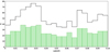 |
Fig. 1 Redshift distribution of the 540 merging systems (green filled histogram) and for all 919 individual galaxies in the merging systems (black histogram). |
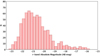 |
Fig. 2 SDSS r-band absolute magnitude distribution of all individual galaxies in the final sample. |
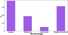 |
Fig. 3 Distribution of galaxy morphology for all individual galaxies in the sample: classifications are spiral, elliptical, lenticular (SO), and highly disturbed (i.e. galaxies that are too disturbed to be included in the other classifications). |
2.2 Imaging data
We compiled data from several surveys spanning the UV, optical, and IR wavelengths. We gathered fully reduced imaging for the FUV and NUV from GALEX8 (GR6/GR7), obtaining images of 1.2° (1450 pixels) in radius. For SDSS9 (DR13), we obtained images for the following optical bands: u, 𝑔, r, i, and ɀ (10 × l3 arcmin2, which corresponds to 2048 × 1489 pixel2). Finally, we used 18.3 × 18.3 arcmin2 (800 × 800pixel2) images for W1, W2, W3, and W4 from WISE10.
3 Results
In this section, we present our semi-automated photometry approach, the complications that arise from automated photometry, and possible solutions. We show the results of our photometry and compare them with available catalogues. Finally, we compare our measurements of M* and SFR with those in the catalogues, and discuss the possible biases.
3.1 Galaxy and merger sequence classification
The 540 mergers of the final sample were classified by morphology and merging stage based on a visual inspection of the SDSS images. The morphological classes of the individual galaxies in the systems are spiral, elliptical, lenticular (SO), and highly disturbed. The last classification includes all galaxies that are too disturbed to be clearly included in any of the other three classifications. An example of each classification is shown in Fig. A.1. Figure 3 shows the distribution of the morphology of the merging galaxies. A large fraction of the sample (34%) is highly disturbed. Most of these galaxies are likely to have been identified as spirals in the past as they presently show very disturbed tidal tails and nuclear regions. Other galaxies show shells, features often associated with mergers involving elliptical galaxies.
Some studies classify mergers based on their separation (Ellison et al. 2008, 2011, 2013; Darg et al. 2010). However, applying this criterion based on component separation does not necessarily imply that mergers are ordered in the correct merging time considering that the distance between the merger components depends on the mass ratio of the components and the particular orbital parameters of each merging system (e.g. relative speeds).
We thus based our classification on a more timeline-like merging sequence. Firstly, we applied the classification prescription in Veilleux et al. (2002, hereafter V02), and then developed a subclassification using a new criterion defined in this work. Veilleux et al. (2002) separate the merging sequence into five merging stages: I (First Approach), where the two galaxies are clearly separated, but are on course to collide. Here we added the additional constraint that the velocity separation is ∆ɀ < 0.002 (∆υ < 500 km s−1); II (First Contact), where the galaxies are overlapping, but show no clear signs of disturbance in their morphology; III (Pre-Merger), where galaxies show strong tidal tails, bridges, and/or shells, but there are still two nuclei clearly observed; IV (Merger), where there is only one nucleus visible (diffuse or compact) and the resulting galaxy shows a very disturbed morphology; and V (Old Merger), where there is only one galaxy with no visible tidal tails, but it shows a disturbed central morphology. Figure 4 shows the V02 classification scheme for a complete merging sequence.
Our new merging sequence is based on the V02 sequence with additional separations tracing a more detailed timeline of the merging process allowing us to explore possible dependences in more detail. We separate the merging stage III into three substages: IIIa (overlap), where the two galaxies overlap and show disturbances; IIIb (disturbed), where the two galaxies show strong tidal tails, bridges, and/or shells, but they are clearly separated (not overlapping); IIIc (double-nucleus), and an intermediate stage between IIIb and IV, where only one galaxy is observed as highly perturbed and shows two clear nuclei. We also separated the merging stage IV into two different stages following the V02 description, but in a more visual way since our galaxies are all in the nearby Universe. Merging stage IVa (diffuse-nucleus) shows a diffuse centre, and IVb (compact-nucleus) shows a compact nucleus. Figure 4 shows an example of our classification.
Figure 5 shows the distribution of merging stages defined by V02 (blue) with our additional definitions (green inserts). Most of the mergers are classified as merging stage III; this is the easiest stage in which to detect a merger because the merger features can be seen most clearly at this stage.
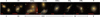 |
Fig. 4 SDSS images of an example merger from each merging stage defined in this study (top), and defined in V02 (bottom). Red lines represent 20″ in each image. |
3.2 Galaxy photometry: problems and solutions
When visualising the images using the WISE interactive website11, it was immediately clear that the galaxies were often much larger than the radii listed in the WISE website tables.
As a first check, we measured the sizes of the mergers using the measuring tool available in the interactive WISE website. Figure 6 compares the radii we measured using the interactive WISE website for W1 with the semi-major axis (rsemi) tabulated in the AllWISE extended sources catalogue. Their rsemi are always heavily underestimated. These smaller radius measurements are likely linked to the low sensitivity of 2MASS, which was used to estimate the apertures for the AllWISE catalogue. This immediately shows that the photometry of mergers listed in the AllWISE catalogue is not accurate, and that the total luminosity is underestimated. For this reason, we decided to perform our own photometry across all the filters we use, not just on the WISE imaging.
Another difficulty arising in mergers is that they can be so disturbed that the usual parameters used when making automated photometric measurements do not extract all the light from the galaxy. Disturbed morphologies, faint tidal tails, and luminous star-forming regions all have to be taken into account when measuring a merging galaxy’s luminosity. Also, since the mergers do not show the same features along the merging sequence, or often with each other, there is no unique set of parameters that can be used to perform the photometry automatically from system to system. Therefore, we are forced to perform the photometry for all the systems, and in all bands, almost completely manually. However, to aid efficiency, we developed a semi-automatic procedure that we describe here.
We started by performing the photometry in the WISE images, using SExtractor (Bertin & Arnouts 1996). For example, as we apply commonly used values for the sky-threshold (3σ) and deblending-threshold (n-deblending = 4), we saw that not all the mergers were included completely within the aperture, hence not all the light was extracted from the source by SExtractor (see Fig. 7, top panel). Also, for some galaxies the same SExtractor set-up extracts only the light of a very bright star-forming region within the merging galaxy (see Fig. 7, bottom panel). Thus, we experimented with various values for the main SExtractor parameters, until we obtained a matrix of possible reasonable parameters (sky-threshold (σ): 1.5, 3, and 5 and n-deblending: 2, 4, 8, 16, and 32). We then repeatedly ran SExtractor on each of our sources, applying each pair of values from the matrix of SExtractor parameters and, in the process, obtaining 15 images per galaxy per filter.
Then each image and its resultant SExtractor apertures were checked visually in order to choose the best SExtractor parameters for each individual galaxy. The best parameters are those that show an aperture that encompasses all of the light from the galaxy, exclude contamination from other sources, and do not exclude any star-forming region that belongs to the galaxy. In the case when two individual galaxies were overlapping, we chose the parameters for which SExtractor shows an aperture that includes both galaxies within one aperture. This could happen in merger stages II and IIIa. We also confirmed that the measured flux does not increase when we increase the size of the aperture in blank regions of the sky.
Some examples of how the parameters affect the result for one system can be found in Fig. 8. The top panel shows how SExtractor separates the galaxy into different regions for σ = 1.5 and n-deblending = 4. The middle panel shows how SExtractor detects the central part of the galaxy only, making an aperture that is too small for σ = 3.0 and n-deblending = 4. Finally, the bottom panel shows how SExtractor successfully detects the galaxy and correctly chooses an aperture which is sufficiently large to enclose all of the light from the galaxy for σ = 5.0 and n-deblending = 4. It is important to note that the case shown in Fig. 8 is only one example, and that the most suitable parameters chosen for this galaxy do not provide acceptable results for other mergers in our sample. More examples are shown in Appendix C. This highlights how redoing the photometry was a necessity for our mergers, and demonstrates that performing automated photometry on these types of complex sources is highly challenging.
Our photometric technique can be summarised as follows. We first check which parameters extract all the light from each galaxy in the WISE bands W1 and W4, and then choose the larger aperture between W1 and W4 and use that aperture size for all filters. The location of the aperture in the rest of the filters is automatically found by Sextractor. In practice, we find that once the best set of parameters is found for a particular galaxy from the W1 image, running SExtractor with these parameters on the other filters results in similar detections. We visually check each filter to ensure that the sources are detected entirely and check for possible contamination, and rerun with alternative parameters from the set if necessary.
To show an example of how unreliable some catalogued measurements can be, we selected a merging galaxy and show the apertures from the different surveys and our aperture measured by SExtractor using the optimal parameters for this galaxy. Figure 9 shows 12 images, the first image is the SDSS ugriɀ image, followed by the 11 filters we use: FUV, NUV, u, g, r, i, z, W1, W2, W3 and W4 (as described in the bottom right corner of each image). For FUV and NUV we show the aperture listed in the GALEX catalogue in cyan. For the ugriɀ images, SDSS shows only one aperture size, which is from the r-band aperture (in magenta); this value is also used by CHANG 15 to correct their W1–3 fluxes. The aperture shown for this galaxy by SDSS is so small that it is barely seen in the figure. For the WISE filters, we show the rsemi values listed in the AllWISE catalogue (in red). Finally, we show our measured aperture (green circle) in all the images. In this case, we selected the aperture size measured for W4 since it is larger than that found for W1. We can see that for all the images the aperture sizes used by the different catalogues are much smaller than the galaxy, while our aperture covers the entire galaxy in all 11 filters.
The final fluxes were corrected for Galactic extinction (Schlafly & Finkbeiner 2011; Yuan et al. 2013) for all filters (except W3 and W4 for which Galactic extinction is negligible). They were also corrected following each survey’s specification. The SDSS u and ɀ bands need a correction of 0.04 and 0.02 mag, respectively, and an extra calibration of 8% for spiral and disc galaxies is needed for W4. In order to take possible systematic uncertainties into account, we added 0.05 in GALEX (Marino et al. 2011), and 0.02 and 0.1 mag in SDSS and WISE (CHANG 15), respectively, to the statistical uncertainties calculated by SExtractor.
To check the reliability of our estimated photometric uncertainties, we performed the following test. For each galaxy, we compared the flux measured in the aperture using our best set of parameters (sky-threshold and n-deblending), as determined by eye. Next we considered the fluxes measured within the apertures using the parameters of the eight nearest neighbouring cells of the matrix of sky-threshold and n-blend parameters. We then calculated the difference between the best flux and the rest of the eight measured fluxes, and calculated the standard deviation of these differences. We conducted this test in one representative band for each survey: NUV from GALEX, r from SDSS, and W1 from WISE. We find that the standard deviation (0.17, 0.007, and 0.10) for these bands is always smaller than the median uncertainty (0.30, 0.234, and 0.15, respectively). Thus, from this test we conclude that our photometric uncertainties are reasonable estimates. However, we know that if we consider more distant cells the merger is frequently not detected, which confirms that fully automated photometry for mergers is not trivial. We compiled useful information from the different surveys in Table B.1 to facilitate the use of the different parameters that are required in the photometry process.
The aperture fluxes measured by us are significantly different from those measured by previous authors. Figure 10 shows a comparison between our aperture flux values (x-axes) for FUV and NUV and the respective values listed in the GALEX catalogue. Most of the galaxies show higher fluxes for our measurements.
Figure 11 shows nine panels comparing our measured fluxes on the x-axis to the CHANG 15 fluxes. The first five panels (from left to right) show the comparison to the SDSS MODELFLUX values, the following three panels show the comparison to WISE W1–3 mpro fluxes corrected by the radius calibration shown by CHANG 15, and the last panel shows the WISE W4 mpro flux which is not corrected by the CHANG 15 calibration. The WISE W1–4 panels show that for a fraction of our sample there are no measurements listed (see the CHANG 15 fluxes equal to 10 Jy). Thus, we increased the number of useful data for this sample. For the first five panels, most of our fluxes are brighter than those listed for MODELFLUX and for W4 mpro. This is due to the larger apertures we use to measure the flux. For the WISE W1–3 filters, we observed that the CHANG 15 values are systematically higher than our fluxes. This could be related to their correction, which increases the flux depending on the radius in the r band of the galaxy. This correction can be adding more flux than needed for this type of galaxy, overcorrecting the flux for these three filters. The fluxes are affected differently depending on the filter, which will create an offset and will also change the shape of the final SED.
Figure 12 shows the comparison between the fluxes measured by SExtractor (x-axes) and the AllWISE table gmag values, which is recommended for extended sources by the WISE team. Our fluxes are higher than those listed in the AllWISE tables due to our larger apertures. For a small fraction of the galaxies at the faint end of W3 and W4 (6% and 10%, respectively), we see that our measurements are lower those listed in the AllWISE tables.
Figure 13 shows the comparison between our W1 photometry measurements on the x-axis and the WISE table W1 gmag values (recommended for extended sources), colour-coded according to the ratio between our aperture radius and the WISE table semi-major axis (rsemi). This clearly shows the dependence of the measured flux on the aperture used during the photometry. For almost all galaxies our measurements give higher fluxes than those listed in the WISE table magnitudes, which is primarily due to our (more correct) larger apertures.
The comparisons between our measured fluxes and those listed in GALEX, SDSS, and WISE do not depend on the morphology of the galaxies or on the stage of the merger. Some of these comparisons can be seen in Fig. D.1.
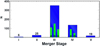 |
Fig. 5 Distribution of merger stages following the classification in V02 (blue), and our own classification (blue plus green). |
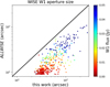 |
Fig. 6 Comparison of our aperture radius value, required to measure all of a galaxy’s light, in the WISE W1 images (x-axis; see text for details) with the rsemi of the AllWISE catalogue. The line of equality is shown with a solid black line and the galaxy symbols are colour-coded according to the total W 1 flux (in Jy). |
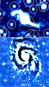 |
Fig. 7 Example of the danger of using the same automated SExtractor photometry on WISE images of the full sample. SExtractor was run with the same parameters on both examples shown. Top: SExtractor finds an aperture that is smaller than the galaxy. Bottom: SExtractor detects the different star-forming regions as separate galaxies and not as a single galaxy. |
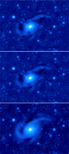 |
Fig. 8 Examples of running SExtractor, with different parameters (changing sky- and deblending-thresholds) on the same galaxy. See text for details. |
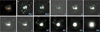 |
Fig. 9 Example of the different apertures used by different surveys and our measurement in all the filters. The first image shows the galaxy in the SDSS u𝑔riɀ bands. The orange line represents 20″. This SDSS image is followed by FUV and NUV from GALEX; u, 𝑔, r, i, and ɀ from SDSS; and W1, W2, W3, and W4 from WISE. Cyan circles show the apertures shown on the GALEX catalogue. Magenta apertures show the small aperture listed in SDSS tables, which is barely seen in the figure. Red apertures are the listed ellipses in AllWISE tables. The aperture we use for all filters, in this case measured from the W4 image, is shown in green. |
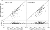 |
Fig. 10 Flux comparison between our measured photometry and the values in the GALEX table. The black line shows equality. The y-axes show the GALEX FUV-NUV flux. The dashed and dotted lines show the 1- and 3-σ deviation from the one-to-one relation, respectively. |
3.3 MAGPHYS: SED fitting to obtain M* and SFR of mergers
We obtained our M* and SFR values using the publicly available SED fitting code MAGPHYS12 (da Cunha et al. 2008). This program fits photometric data from UV to submillimetre wavelengths. We used the 2003 libraries recommended by their website, which assembles 50 000 stellar population template spectra (Bruzual & Charlot 2003) for the optical photometric library and other 50 000 polycyclic aromatic hydrocarbon (PAH) plus dust emission template spectra for the infrared photometric library. MAGPHYS models galaxy SEDs according to the redshift of the given sample and uses a Bayesian approach to interpret the SEDs so as to statistically derive different galaxy properties such as M* SFR, and dust mass, among other quantities.
In order to obtain more accurate estimations of the M* and the SFR of our galaxies, our sample was chosen such that all mergers have available imaging covering the FUV, NUV, u, 𝑔, r, i, ɀ, W1, W2, W3, and W4. When a merging galaxy did not show flux in some filter (occasionally FUV, NUV, or W4), we set the flux to −99.0 and an uncertainty of 3-σ of the average error found for that filter. In this manner, MAGPHYS will consider this flux as an upper limit.
The SED fits show a median  and a mean of 1.9. Some SED fitting examples are shown in Fig. E.1. The top panel of Fig. 14 shows the distribution of the estimated M* (in red); for our merger sample the median value is log(M*/M⊙) = 10.28 ± 0.76. The resulting SFR have a median of log(SFR/M⊙ yr−1) = 0.51 ± 0.86 with the distribution shown in the bottom panel of Fig. 14 in blue.
We also estimated M* and SFR using only the optical and near-infrared (NIR) data in order to compare these results to the CHANG 15 catalogue who use the same limited numbers of filters. For this sample, we obtain a mean and a median of  and 0.25 for the SED fits. A lower
  could result because MAGPHYS finds it easier to fit to fewer data points, but the fits may also be less accurate since the code is missing information from the young population of the merging galaxy. When we include GALEX data, both M* and SFR estimates are very similar to those derived using SDSS+WISE only (orange and cyan histograms in Fig. 14, respectively).
In Figs. E.1 and E.2, we show some examples of the SED fits for the sample using all eleven filters and SDSS+WISE only, respectively.
3.4 M* and SFR comparison to the CHANG 15 catalogue
We compare the results obtained by MAGPHYS using all the filters with those obtained using only SDSS+WISE (see Fig. 15). We can see that they correlate and have a scatter of 0.1 dex for M* (top panel) and 0.2 dex for SFR (bottom panel), with no apparent systematic offsets. The scatter may be larger for SFR compared to M* because UV is a sensitive tracer of recent star formation. This means that including GALEX may not cause large differences in measurements for the majority of the sources, but it can lead to differences as large as 10 and 15 times for M* and SFR, respectively, in individual galaxies. We colour-coded the merging galaxies by morphology in order to look for dependences. The scatter in M* is dominated by spirals and highly disturbed galaxies; instead, for the SFR the scatter is similar for all morphologies.
Figure 16 shows the comparison between our M* (left) and SFR (right) results and the values listed in the CHANG 15 catalogue. We cross-matched our mergers to this catalogue using a distance limit of 5″, where all coordinates come from SDSS. The mean size of our mergers is 42″, thus the distance limit is very small compared to the size of the merging galaxies. In the case of overlapping galaxies, we only considered the one with the minimum distance.
Since we also have the SDSS+WISE results, we can directly compare our results to the CHANG 15 values. In both cases MAGPHYS is used to estimate M* and SFR. The only difference is that CHANG 15 used the measurements shown in SDSS and AllWISE tables with an additional correction for W1–3 fluxes based on the aperture size in the SDSS r band, whereas we use our own semi-automated photometric approach. Thus, any differences that arise are primarily the result of the photometric methodology. Stellar masses show good agreement for most of the sample with a scatter of 0.5 dex, considering only CHANG 15 sources with M* > 107 M⊙, and a scatter of 0.76 dex for SFR, considering only CHANG 15 sources with SFR > 10−3 M⊙ yr−1. The comparisons of M* and SFR show no dependence on merger stage or separation (see Fig. F.1). The comparison of SFRs shows a large scatter, which indicates that SFRs are more affected by small differences in photometry compared to M* There are many galaxies with very low SFRs estimated by CHANG 15, which can be underestimations of this property either because the UV emission is not considered and/or because of overcorrections of the W1, W2, and W3 fluxes. This leads to changing the SED shape affecting the M* and SFR estimates, resulting in differences up to 500 times in M* and 5000 times in SFR.
The correlation does not clearly depend on morphology, but the scatter of M* is dominated by spirals and highly disturbed galaxies. For the SFR, a large fraction of spirals and highly disturbed galaxies are close to the one-to-one relation. However, there is still a large scatter, similar to ellipticals and lenticular galaxies.
We made a linear fit to the distribution of data points in Fig. 16. The parameters of the best fit and the scatter about that fit are provided in Table 1.
In order to better understand the largest differences between our results and CHANG 15, we plotted the SEDs of some galaxies showing some of the largest differences for M* and/or SFR.
Figure 17 shows the SEDs of the galaxies shown in Fig. 16 indicated by the same symbol shown in the top right corner of each SED. Next to each SED, we show the u𝑔riɀ image of each galaxy with the aperture we use in green, and the SDSS aperture used by CHANG 15 in magenta.
From top to bottom, as shown in Fig. 17:
 The upper panel shows that most of the fluxes shown by CHANG 15 are very similar to our measurements, even when their aperture is much smaller than ours. However, the u and W4 shows lower values for CHANG 15. This can be the reason why their SFR value is much lower than ours, since these wavelengths show the emission and re-emission of young star formation, respectively.
 The second panel shows a galaxy that had not been measured accurately either by SDSS or WISE. The SDSS aperture is very small, barely seen in the u𝑔riɀ image. Thus, our M* and SFR values are very different to the CHANG 15 values.
 The third panel shows that the SDSS photometry shows a very different shape for the SED. However, the fluxes are not very different at these wavelengths. On the other hand, CHANG 15 shows lower fluxes for WISE compared to ours. Furthermore, there is no W4 flux shown by CHANG 15. The similarity in the SDSS fluxes might be the origin of the similarity in M*, and the higher WISE fluxes of our measurements can explain our higher SFR estimate.
◊ The lower panel shows a very small aperture for SDSS, showing very low fluxes compared to our measurements. For WISE, however, the measurements are very similar. This results in very different M* and SFR estimates.
This shows that there are several factors affecting the difference in the results, such as differences in the photometric data of one survey compared to the other, low measurements in all of the filters, or different measurements made in one or two filters which change the shape of the SED. Hence, mergers must be studied with extreme caution if the catalogued values are to be used.
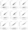 |
Fig. 11 Comparison of our aperture flux values with those listed by CHANG 15 for all galaxies common to our samples. Specifically, we use the SDSS MODELFLUX values and the WISE mpro fluxes from CHANG 15. The solid line in each main panel shows the line of equality and each small panel shows the difference between the two axes. Data points at the highest y-axis values in each main panel represent galaxies with fluxes measured by us, but not by CHANG 15. The dashed and dotted lines show the 1- and 3-σ deviation from the one-to-one relation, respectively. |
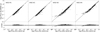 |
Fig. 12 Flux comparison between our measured photometry and the values in the WISE table. The black line shows equality. The y-axes show the WISE gmag flux conversion. The dashed and dotted lines show the 1- and 3-σ deviation from the one-to-one relation, respectively. |
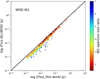 |
Fig. 13 Comparison of our total aperture flux (Jy) value and that listed in the WISE tables for all galaxies in our sample. Symbols are colour-coded according to the ratio of our measured aperture size to that applied by the WISE team, and the black line shows equality. |
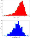 |
Fig. 14 Distribution of M* (top) and SFR (bottom) obtained by MAG-PHYS for all individual galaxies in our sample. The red and blue histograms show the M* and SFR distribution using all 11 filters, and the orange and cyan histograms show the results using SDSS+WISE only. |
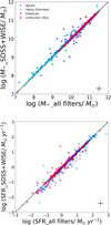 |
Fig. 15 Comparison of the M* (top) and SFR (bottom) estimated by MAGPHYS when using all filters (see text) on the x-axis and only SDSS+WISE filters on the y-axis. The typical error is shown in the bottom right corner of each panel. The sample is colour-coded according to morphology as indicated in the legend. |
Best-fit parameters obtained from the comparison between our M* and SFR results and those listed in the CHANG 15 catalogue.
3.5 Testing common estimators of M* and SFR
In this section, we consider how various M* and SFR indicators perform on samples of mergers. The indicators we show in this section were derived using different methods to those used in this study, but using some of the filters that we use. Thus, we can compare commonly used M* and SFR indicators from the literature with our results measured using MAGPHYS. The M* and SFR computed for this section were calculated using our new photometric values and the relations from the literature. We start by comparing M* indicators.
We also contrast our MAGPHYS-derived M* values with those estimated from one- or two-band photometry by Cluver et al. (2014, hereafter CL 14), Bell et al. (2003, hereafter B03), and Taylor et al. (2011, hereafter T11). CL 14 have studied two of their equatorial fields in the Galaxy and Mass Assembly (GAMA) Survey. They note that ‘the typical W1 1-σ isophotal radius is more than a factor of ~2 in scale compared to the equivalent 2MASS Ks-band isophotal radius’, and that WISE gmags should be used with caution since no deblending or star subtraction has been made in WISE tables, which is further reason to apply our semi-automatic approach. They also show empirical relations between the M* derived from synthetic stellar population models and W1 and W2 colours and W1 luminosity, which they separate into three equations following the form logMstellar/LW1 = a(W1 − W2) − b, with LW1(L⊙) = 10−0.4(Mw1−3.24), where MW1 is the absolute magnitude in W1. For low-redshift sources a and b are −2.54 and 0.17, respectively; for star-forming galaxies a and b are 0.04 and −1.93, repectively; and a = −1.96 and b = 0.03 are the best-fit values for the entire sample.
Figure 18 shows the comparison between our M* and the estimates using the CL 14 relations. The left panel shows the M* estimated using the CL 14 relation for low-redshift galaxies, and the right panel shows the M* estimations using the CL 14 relation for their entire sample, and using the star-forming relation for star-forming galaxies. Both methods tend to provide higher values of M* compared to our results, and with large scatter (1.1 dex and 1.0 dex, respectively), leading to differences of up to a factor of 1000. The correlations of these comparisons do not show a clear dependence on the morphology of the merging galaxies, but the scatter is dominated by spirals and highly disturbed galaxies.
The relation shown by B03 is frequently used, this relates the M* to optical colours following log(M*/Lr) = −0.15 + 0.93(𝑔 − r)(1) and log(M*/Lr) = −0.306 + 1.097(𝑔 − r)(2) for galaxies in the range 0.3 < (𝑔 − r) < 1, with Lr being the luminosity (L⊙) in the r band. Figure 19 (left panel) shows the relation between log(M*/Lr) and the (𝑔-r) colour. Equations (1) and (2) from B03 are shown by the orange and brown lines, respectively. Our best fit (in green) shows a steeper slope than for B03 sample: log(M*/Lr) =0.9+l.69(𝑔 − r) and redder colours for a large fraction of our sample. This could be related to the higher dust mass of merging galaxies compared to unperturbed galaxies.
Figure 19 (right panel) shows the relation between the M*/Li and the (𝑔-i) colour. The orange line shows the relation determined by T11 for the GAMA sample: log(M*/Li) = −0.68 + 0.70(𝑔-i), with Li being the luminosity in the i band, in L⊙. Our best fit (green line) shows a steeper slope, log(M*/Li) = 0.96 + 0.90(𝑔-i), but no offset with colour. This suggests that T11 can properly correct for dust, as they also use near-infrared filters (WISE), and they additionally include Herschel. The large scatter could be due to different photometry used for their and our calculations.
These two relations do not show a clear dependence on morphology and the scatter is large for all morphologies. However, spirals and highly disturbed galaxies show larger scatter compared to elliptical and lenticular galaxies.
We now compare our MAGPHYS-derived SFR results to those estimated by CL 14, Lee et al. (20l3), Jarrett et al. (20l3), CHANG 15, and Janowiecki et al. (20l7, hereafter J17). CL 14 also present a relation between a dust-corrected Hα-derived SFR and W3 and W4 luminosities separately:
log  ,
,
log  .
.
Figure 20 shows the comparison between our SFR and the estimates from the CL 14 relations for W3 (left panel) and for W4 (right panel). CL 14 SFR correlate closely to our results, showing larger scatters for SFR estimated from W3 compared to estimations from W4 (0.5 compared to 0.4, respectively). This could occur because W3 is more affected by PAH emission, as shown in previous studies (Jarrett et al. 20l3, CL 14, CHANG 15). It is important to note that even if they seem to relate closely, the estimations can lead to differences of up to a factor of 50 for the W4 relation and a factor of 500 for the W3 relation.
The scatter in the results using the W3 relation is large for all morphologies. Nevertheless, a large fraction of spirals and highly disturbed galaxies seem to be closer to the one-to-one relation. The comparison to the SFR using the W4 filter show no dependence on mophology.
The left panel of Fig. 21 shows the relation between the SFR and the luminosity in W4. We show different relations found in the literature. Lee et al. (2013) show two relations, a non-linear (orange dotted line) and a linear relation (orange solid line). The brown dashed line shows the relation found by Jarrett et al. (2013) and the green line shows the relation found by CHANG 15. Our relation seems to be between the Lee et al. (20l3) and CHANG 15 relations. There is a large scatter (~0.4 for the Lee et al. 2013 equations, and ~0.5 for Jarrett et al. 2013 and CHANG 15), showing higher SFR for the same LW4, which might indicate that Lw4 does not fully trace all the SFR of the galaxy. This result does not depend on the morphology of the merging galaxy.
Figure 21 right panel shows a comparison of the SFR we derive from MAGPHYS and that derived using the SFR estimator of J17. The J17 approach combines the SFR from the NUV light and the attenuated light in W4 following SFR = SFRNUV + SFRw4, with SFRNUV (M⊙ yr−1) = 10−28.165 * LNUV (erg s−1 Hz−1) from Schiminovich et al. (2007) and SFRw4 (M⊙ yr−1) = 7.50 × 10⁻¹⁰(Lw4 − 0.04 Lw1)(L⊙) from Jarrett et al. (2013) with an extra correction for stellar contamination. Our results and those of J17 both show a tight correlation for a large fraction of the sample, except for galaxies with low SFR. The correlation and scatter are very similar for all morphological classifications.
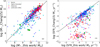 |
Fig. 16 Comparison between our M* (left panel) and SFR (right panel) estimates to the estimates listed by CHANG 15. The typical error is shown in the bottom right corner of each main panel. Data points at the lowest y-axis values in the left panel represent galaxies with the minimum value set by CHANG 15. These data points are not considered for the fits. The merging galaxies are coloured by morphology as shown in the legend. |
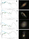 |
Fig. 17 SED and u𝑔riɀ images for galaxies with large differences between our M* and SFR results and the CHANG 15 results. The symbol shown in the top right corner of each SED corresponds to the galaxy symbol in Fig. 16. The black and blue lines show the attenuated and unattenuated SED fit to our measurements in green. The red dots show the fluxes used by CHANG 15. The u𝑔riɀ image show the apertures measured in our study in green and the one measured by SDSS in magenta. The red line represents 20″ in each image. |
3.6 Colour-morphology relation
The mid-infrared colour-colour relation distinguishes galaxies by morphology, luminosity, and AGN content. Figure 22 shows the colour-colour relation (Jarrett et al. 2011, 2017; Cluver et al. 2014), which allows us to identify galaxies as AGNs and ULIRGs, and also classifies galaxies by morphology, for example spheroids (ellipticals and lenticulars) and discs (intermediate and star-forming). The lines shown in the figure follow the separations shown by CL 14.
We can see that, overall, merging galaxy morphologies differentiate similarly to unperturbed galaxies on the WISE colour-colour diagram. Elliptical (red) and lenticular (magenta) galaxies are mostly in the spheroid region, and spiral (blue) and highly disturbed (cyan) galaxies are in the disc region. We can see a high number density of data points in the star-forming disc region where we expect to find spirals and starburst galaxies. It is also important to note that, as expected, merging galaxies can be found spread over this plot; we can see blue ellipticals and red spirals as they change colour due to the merging process.
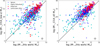 |
Fig. 18 Comparison of our M* values (derived from our MAGPHYS fits to data in GALEX, SDSS, and WISE filters) to those estimated using only WISE W1 and W2 photometry combined with the relations provided in CL14. The left panel shows the comparison to the relation for low-redshift sources, and the right panel shows the comparison to the relation for star-forming galaxies (see text). The typical error is shown in the bottom right corner of each panel. The coloured symbols show the morphology of the merging galaxies as described in the legend. |
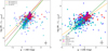 |
Fig. 19 Comparing our M* results to B03. Left: ratio of M* to light versus the colour relation from B03. The orange line shows Eq. (1) and the brown line shows Eq. (2) from B03. Our best fit is shown in green. Right: ratio of M* to light versus colour relation from T11. The orange line shows M* -colour relation from T11. Our best fit is shown in green. The typical error is shown in the bottom right corner of each panel. The merging galaxies are colour-coded according to their morphology as indicated in the legend. |
3.7 Specific star formation rate
In order to look for a specific star formation rate (sSFR) indicator using one or two photometric bands, we look for a relation between this parameter and a combination of the stellar component and the dust/obscured star-forming component, which can be traced by the mid-infrared colour W1–W4 (Vega mag) from the WISE filters. Figure 23 shows the relation found for our merger sample, which is described by Eq. (1):
 (1)
(1)
The scatter of this relation is similar for all morphologies except for lenticular galaxies, which show a smaller (0.2 dex) scatter compared to that shown by the other morphologies (0.5 dex).
4 Public catalogue
The public catalogue shows all the information we have used for our results. We list all the information of the merging galaxies, showing the same name for pairs and adding a ‘b’ to the name for the companion. Coordinates are centred in the individual merging galaxy, coordinates of overlapping galaxies are centred in each of their nuclei. We present the morphology and merger stage as classified in this study. We also provide the fluxes and their errors as measured and explained in Sect. 3.2. Stellar masses (M*) and star formation rates (SFR) are listed in log-scale, and we also provide the χ2 values of each fit made using MAGPHYS. This catalogue will be publicly available on the ViZiER website13; a direct link to the catalogue can be found in the online data from ASO/NASA Astrophysics Data System. See Table 2 for the description of the catalogue’s columns.
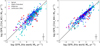 |
Fig. 20 Comparison of our SFR values (derived from our MAGPHYS fits to data in GALEX, SDSS, and WISE filters) to those estimated using only WISE W3 and W4 photometry combined with the relations provided in CL 14. The left panel shows the comparison to the relation using W3, and the right panel shows the comparison to the relation using W4. The typical error is shown in the bottom right corner of each panel. The sample is colour-coded according to morphology, as shown in the legend. |
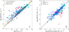 |
Fig. 21 Comparing out SFR results to the literature. Left panel: relation between the SFR and the W4 luminosity (LW4/L⊙). The lines show different relations from the literature. The orange dotted line shows the non-linear relation found by Lee et al. (2013), while the orange solid line shows the linear relation from the same study. The brown dashed line shows the relation by Jarrett et al. (2013) and the green line shows the relation found by CHANG 15. Right panel: comparison between our MAGPHYS SFR results and the calculation using the SFR relation defined by J17. The black line shows the equality line. The typical error is shown in the bottom right corner of each panel. The coloured symbols represent the morphology of the merging galaxies, as described in the legend. |
5 Discussion and conclusions
We have assembled a sample of 540 mergers in isolated environments. The galaxies forming part of the merger were constrained to have similar redshift, which ensures that we are including only galaxies that could merge (i.e. we exclude clear cases of fly-bys). The mergers have been classified by morphology and we have also classified the mergers according to their current phase in the merging process.
We performed photometry in a semi-automated manner in order to extract the flux of the entire galaxy. We find this is necessary as the automated photometry from publicly available catalogues is unreliable for this type of galaxy. Our semi-automated photometry was performed in 11 bands, including ultraviolet (FUV and NUV from GALEX), optical (u, 𝑔, r, i, and ɀ from SDSS), and the near-infrared (W1, W2, W3, and W4 from WISE).
We find that most of the galaxies show higher fluxes using our semi-automated photometry compared to the GALEX, SDSS, and AllWISE catalogues. This is a result of the larger apertures that we find are required in order to capture all of the galaxy’s light in comparison to the fluxes from these catalogues in the literature. This demonstrates that automated methods are not efficient in extracting all of the light in merging galaxies, often missing the light in the outskirts where tidal features may be found, and breaking up the galaxy into individual objects instead of recognising they are from the same galaxy (e.g. star-forming regions). Also, we find that radial the corrections performed by CHANG 15, which were designed to correct for aperture effects, seem to result in overestimating the flux for W1–3. This shows that corrections of this type may have poor accuracy in merging galaxies. These combined results have convinced us to pursue a less automated approach to perform the photometry in order to make sure that we are measuring the light of the entire galaxy in all the filters mentioned above.
Comparing the results for M* and SFR using the same method (MAGPHYS) but varying the number of filters used as an input (GALEX+SDSS+WISE versus SDSS+WISE), the one-to-one relations are tight for most of the sample, while it can lead to differences of a factor of 10 for M* and 15 for SFR for individual galaxies. This indicates that UV is clearly important to the SFR estimation, as might be expected, and that it is significant for M* estimations. When we compare our measured fluxes to the CHANG 15 fluxes, we find that our measurements are higher than theirs, except for W1–3. This might be a result of the aperture correction, which tends to overcorrect the fluxes on these filters. This can cause MAGPHYS to fit an altered SED resulting in our measurements having lower M* and higher SFR.
We note that the scatter in M* and SFR is smaller than the scatter seen when comparing fluxes. This suggests that the SED fitting is smoothing out some of the scatter seen in the fluxes, which could be partially related to the resolution of some of the filters that contribute the most to M* and SFR estimations. However, it is important to note that even when the scatter appears to be small, the difference in photometry for some of the galaxies can lead to differences in M* of a factor of 1000 and a factor of 10 000 for SFR. This suggests that the previous values in the literature should be used with caution, and that adequate photometry must be conducted for these types of galaxies before estimating M* and SFR.
The differences in photometry results show no clear dependence on either morphology or merger stage. The only dependence is on the aperture size used when extracting the light from each source. There is also no clear dependence on morphology or merger stage in the M* and SFR estimates, which leads us to conclude that the major factor affecting our results is the photometry performed.
The M* and SFR indicators based on optical colours and NIR and/or NUV fluxes, respectively, also show large scatter. For the M* indicators, our results show lower log(M*/Lr) for the same colours compared to the B03 relations. On the other hand, our M* shows a closer correlation to the T11 M* indicator, which is also based on SED fitting of photometric data spanning from the UV to the far-infrared, but using different photometry. For the SFR indicators, the scatter seems to be larger mainly for highly disturbed and elliptical galaxies. This can also be related to the photometry used at these wavelengths; the fluxes in the NIR filters can be underestimated (for highly disturbed galaxies) or the NUV fluxes not considered for some of the indicators (for both highly disturbed and elliptical galaxies). It is important to note that these catalogues and indicators have been optimised for statistical studies. Thus, it is not surprising that they show issues for mergers’ estimations.
The near-infrared colour-colour diagram separates the morphologies of our sample as it is designed to do. However, we can see different morphologies in the various regions of the colour-colour diagram, suggesting that these galaxies go through colour changes when they are involved in a merging process. Also, we observe that mergers in this diagram are not mainly located in the AGN region (above the magenta line). This suggests either that not many mergers host an AGN or that the AGN in mergers are not luminous enough to outshine the brightness of the hosting merging galaxy. This will be discussed further in Paper II, as will the SF enhancement of mergers and their location in the M*–SFR plane separated by merger stage.
Finally, the estimation of sSFR from W1-W4 colours is only recommended for lenticular galaxies as other morphologies show larger scatter. Instead, sSFR should be estimated using M* from W1 (CL 14) and SFR from W4 (CL 14).
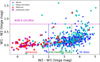 |
Fig. 22 WISE colour–colour diagram showing morphology separation, as in Fig. 5 of CL 14, where galaxies can be classified as Spheroids, Intermediate discs, star-forming discs, and AGNs and (U)LIRGs. Our merging galaxies are colour-coded according to morphology, as indicated in the legend. |
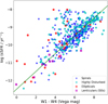 |
Fig. 23 sSFR-WISE colour relation for mergers. The green line shows the best fit to our sample (see text). The coloured symbols show the morphology of our mergers (see legend). |
Output catalogue.
Acknowledgements
We would like to thank the referee for a constructive report which helped us improve this manuscript. P.C-C. was supported by CONICYT (Chile) through Programa Nacional de Becas de Doctorado 2014 folio 21140882. N.N. acknowledges support from Conicyt (PIA ACT172033, Fondecyt 1171506, and BASAL AFB-170002). S.K.Y. acknowledges support from the Korean National Research Foundation (NRF-2017R1A2A1A05001116). This study was performed under the umbrella of the joint collaboration between Yonsei University Observatory and the Korean Astronomy and Space Science Institute. G.O. acknowledges the support provided by CONICYT (Chile) through FONDECYT postdoctoral research grant no 3170942. R.L. acknowledges support from Comité Mixto ESO-GOBIERNO DE CHILE, GEMINI-CONICYT FUND 32130024, and FONDECYT Grant 3130558. T.M.H. acknowledges the support from the Chinese Academy of Sciences(CAS) and the National Commission for Scientific and Technological Research of Chile (CONICYT) through a CAS-CONICYT Joint Postdoctoral Fellowship administered by the CAS South America Center for Astronomy (CASSACA) in Santiago, Chile. We acknowledge the use of the following databases and codes: ARP (http://arpgalaxy.com), GZ (http://data.galaxyzoo.org), VV (www.sai.msu.su/sn/vv), GOALS (http://goals.ipac.caltech.edu), GALEX (http://galex.stsci.edu/data/), SDSS (https://dr13.sdss.org/sas/dr13/), WISE (http://irsa.ipac.caltech.edu/applications/wise/), Chang et al. 2015 catalogue (https://yuyenchang.github.io/index.html), MPA-JHU (https://www.sdss3.org/dr10/spectro/galaxy_mpajhu.php), NSA (http://www.nsatlas.org/), SExtractor (https://www.astromatic.net/software/sextractor), and MAGPHYS (http://www.iap.fr/magphys/).
Appendix A Examples of morphology
In Sect. 3.1, we show the distribution of the galaxy morphologies as classified in this study. Here we present an example of each morphology classification. Figure A.1 shows, from top to bottom, a spiral, an elliptical, a lenticular (S0), and a highly disturbed galaxy from our merger sample. Specifically, to be classified as a spiral, galaxies have to show clear spiral arms not heavily perturbed. Ellipticals show red colours and round shapes with a bright nucleus. Lenticular galaxies show similar morphologies to ellipticals, but they all show a clear disc. Finally, highly disturbed galaxies are those that cannot be classified in any of the previous classes. These galaxies could show highly perturbed spiral arms, various shells, tidal features, among others.
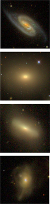 |
Fig. A.1 Examples of the morphology classification. From top to bottom: spiral, elliptical, lenticular, and highly disturbed galaxies. |
Appendix B Survey parameters
Relevant parameters of the filters and images used from the different surveys. 1All-sky 2Deep, and 3Medium Imaging Surveys from GALEX.
To perform the photometry, we searched for the relevant parameters from each survey. We assembled Table B.1 with the reference information used in these surveys.
Appendix C Examples of apertures
Here, we show more examples of the different apertures measured by SExtractor depending on the parameters σ and n-deblending (see Sect. 3.2). Each figure shows three examples for each galaxy using different σ and n-deblending. We show the best aperture at the bottom of each figure.
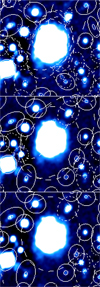 |
Fig. C.1 From top to bottom: σ = 1.5, n-deblending=32; σ = 5.0, n-deblending= 32; σ = 3.0, n-deblending=2. |
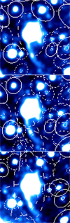 |
Fig. C.2 From top to bottom: σ = 1.5, n-deblending=2; σ = 1.5, n-deblending=32; σ = 1.5, n-deblending=4. |
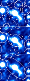 |
Fig. C.3 From top to bottom: σ = 1.5, n-deblending=32; σ = 5.0, n-deblending=32; σ = 5.0, n-deblending=2. |
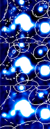 |
Fig. C.4 From top to bottom: σ = 1.5, n-deblending=32; σ = 3.0, n-deblending=32; σ = 3.0, n-deblending=4. |
Appendix D Fluxes comparisons according to different parameters
In Sect. 3.2, we showed the comparison between our measured GALEX NUV fluxes and the GALEX GR6/GR7 catalogue, the SDSS DR 13 r-band fluxes of our measurements and the values listed by CHANG 15, and our measured WISE W1 fluxes and the catalogued values shown in AllWISE tabulated as gmag. Here we colour-coded the comparisons in order to look for any dependences in morphology, merger stage, or photometry flag. The photometry flag shows whether the apertures, measured by our semi-automated method, are completely separated or joined (both galaxies are within the same aperture).
 |
Fig. D.1 Comparison between our GALEX NUV (top panels), SDSS r band (middle panels), and WISE W1 (bottom panels) measured fluxes and GALEX, SDSS, and AllWISE catalogued values. Colour-coded according to morphology (left panels), merger stage (middle panels), and photometry flag (right panels). |
Figure D.1 shows the fluxes we measured from GALEX NUV (top row), SDSS r-band (middle row), and WISE W1 images (bottom row) compared to the values catalogued by GALEX, SDSS, and AllWISE. They are colour-coded according to morphology (left panels), merger stage (centre panels), and photometry flag (right panels). The correlations do not show a clear dependence on any of these parameters. However, spirals and highly disturbed galaxies show a larger scatter. The scatter in the SDSS (centre panel, middle row) is dominated by merging galaxies at merger stage IIIb, where a large fraction of the merging galaxies are either spiral or highly disturbed. This leads to the conclusion that differences in these values are related mainly to the photometry performed.
Appendix E MAGPHYS SED fits
Some examples of fitted SEDs are shown in Figures E.1 and E.2. The figures show six examples of MAGPHYS SED fit results. Each row shows the SED fits of the same object, using all the filters (GALEX, SDSS, and WISE) on the left and the SED fits only using SDSS and WISE on the right. The top panel of each fit shows the photometric points in red, the best-fit SED in black, and the unattenuated SED in blue. The reduced chi-squared (χ2) of the fit is shown in the top right corner of each main panel. The panel below shows the residual between the fit and the photometric points. In the lower panel of each fit, we show four probability distribution functions (PDFs) of some of the parameters estimated by MAGPHYS. From left to right, we show the PDFs of the M*, the sSFR, the SFR, and the dust mass (Mdust).
 |
Fig. E.1 Examples of MAGPHYS SED fits for some of our mergers using GALEX+SDSS+WISE filters (left) and SDSS+WISE filters (right). We show the SED fits for the same object in each row. In the upper panel, the red points show our photometric data, the black curve shows the best-fit SED to the photometry, and the blue curve shows the unattenuated SED. In the top right corner of each panel the |

Appendix F Stellar Masses comparison according to different parameters
We present some comparisons shown in Sect. 3.4; we colour-coded the different parameters to look for any dependences. Figure F.1 shows the comparison between our M* (top) and SFR (bottom) results and those of CHANG 15, colour-coded according to merger stage (left panel) and photometry flag (right panel). We can see that the correlations do not show any dependence in merger stage or photometry flag.
 |
Fig. F.1 Comparison between the M* (top panels) and SFR (bottom panels) estimated by MAGPHYS using the SDSS+WISE filters only and the CHANG 15 results, colour-coded according to merger stage (left panels) and photometry flag (right panels). |
References
- Arp, H. 1966, ApJS, 14, 1 [NASA ADS] [CrossRef] [Google Scholar]
- Bell, E. F., McIntosh, D. H., Katz, N., & Weinberg, M. D. 2003, ApJS, 149, 289 [Google Scholar]
- Bertin, E., & Arnouts, S. 1996, A&AS, 117, 393 [NASA ADS] [CrossRef] [EDP Sciences] [Google Scholar]
- Bruzual, G., & Charlot, S. 2003, MNRAS, 344, 1000 [NASA ADS] [CrossRef] [Google Scholar]
- Chang, Y.-Y., van der Wel, A., da Cunha, E., & Rix, H.-W. 2015, ApJS, 219, 8 [Google Scholar]
- Cluver, M. E., Jarrett, T. H., Hopkins, A. M., et al. 2014, ApJ, 782, 90 [Google Scholar]
- da Cunha, E., Charlot, S., & Elbaz, D. 2008, MNRAS, 388, 1595 [Google Scholar]
- Daddi, E., Dickinson, M., Morrison, G., et al. 2007, ApJ, 670, 156 [NASA ADS] [CrossRef] [Google Scholar]
- Darg, D. W., Kaviraj, S., Lintott, C. J., et al. 2010, MNRAS, 401, 1552 [NASA ADS] [CrossRef] [Google Scholar]
- Di Matteo, T., Springel, V., & Hernquist, L. 2005, Nature, 433, 604 [NASA ADS] [CrossRef] [Google Scholar]
- Di Matteo, P., Bournaud, F., Martig, M., et al. 2008, A&A, 492, 31 [NASA ADS] [CrossRef] [EDP Sciences] [Google Scholar]
- Elbaz, D., Daddi, E., Le Borgne, D., et al. 2007, A&A, 468, 33 [NASA ADS] [CrossRef] [EDP Sciences] [Google Scholar]
- Ellison, S. L., Patton, D. R., Simard, L., & McConnachie, A. W. 2008, AJ, 135, 1877 [NASA ADS] [CrossRef] [Google Scholar]
- Ellison, S. L., Patton, D. R., Mendel, J. T., & Scudder, J. M. 2011, MNRAS, 418, 2043 [NASA ADS] [CrossRef] [Google Scholar]
- Ellison, S. L., Mendel, J. T., Patton, D. R., & Scudder, J. M. 2013, MNRAS, 435, 3627 [CrossRef] [Google Scholar]
- Fensch, J., Renaud, F., Bournaud, F., et al. 2017, MNRAS, 465, 1934 [NASA ADS] [CrossRef] [Google Scholar]
- Holincheck, A. J., Wallin, J. F., Borne, K., et al. 2016, MNRAS, 459, 720 [NASA ADS] [CrossRef] [Google Scholar]
- Hopkins, P. F., Hernquist, L., Cox, T. J., Younger, J. D., & Besla, G. 2008, ApJ, 688, 757 [Google Scholar]
- Janowiecki, S., Catinella, B., Cortese, L., et al. 2017, MNRAS, 466, 4795 [NASA ADS] [Google Scholar]
- Jarrett, T. H., Cohen, M., Masci, F., et al. 2011, ApJ, 735, 112 [Google Scholar]
- Jarrett, T. H., Masci, F., Tsai, C. W., et al. 2013, AJ, 145, 6 [Google Scholar]
- Jarrett, T. H., Cluver, M. E., Magoulas, C., et al. 2017, ApJ, 836, 182 [Google Scholar]
- Karim, A., Schinnerer, E., Martínez-Sansigre, A., et al. 2011, ApJ, 730, 61 [Google Scholar]
- Kartaltepe, J. S., Sanders, D. B., Scoville, N. Z., et al. 2007, ApJS, 172, 320 [NASA ADS] [CrossRef] [Google Scholar]
- Larson, R. B., & Tinsley, B. M. 1978, ApJ, 219, 46 [Google Scholar]
- Lee, J. C., Hwang, H. S., & Ko, J. 2013, ApJ, 774, 62 [NASA ADS] [CrossRef] [Google Scholar]
- Marino, A., Rampazzo, R., Bianchi, L., et al. 2011, MNRAS, 411, 311 [CrossRef] [Google Scholar]
- Mihos, J. C., & Hernquist, L. 1994a, ApJ, 425, L13 [Google Scholar]
- Mihos, J. C., & Hernquist, L. 1994b, ApJ, 431, L9 [NASA ADS] [CrossRef] [Google Scholar]
- Noeske, K. G., Weiner, B. J., Faber, S. M., et al. 2007, ApJ, 660, L43 [CrossRef] [Google Scholar]
- Pannella, M., Carilli, C. L., Daddi, E., et al. 2009, ApJ, 698, L116 [Google Scholar]
- Pannella, M., Elbaz, D., Daddi, E., et al. 2015, ApJ, 807, 141 [Google Scholar]
- Park, J., Smith, R., & Yi, S. K. 2017, ApJ, 845, 128 [NASA ADS] [CrossRef] [Google Scholar]
- Renzini, A., & Peng, Y.-j. 2015, ApJ, 801, L29 [NASA ADS] [CrossRef] [Google Scholar]
- Rodighiero, G., Daddi, E., Baronchelli, i., et al. 2011, ApJ, 739, L40 [CrossRef] [Google Scholar]
- Rodighiero, G., Renzini, A., Daddi, E., et al. 2014, MNRAS, 443, 19 [Google Scholar]
- Sanders, D. B., Mazzarella, J. M., Kim, D.-C., Surace, J. A., & Soifer, B. T. 2003, AJ, 126, 1607 [Google Scholar]
- Schiminovich, D., Wyder, T. K., Martin, D. C., et al. 2007, ApJS, 173, 315 [Google Scholar]
- Schlafly, E. F., & Finkbeiner, D. P. 2011, ApJ, 737, 103 [Google Scholar]
- Schreiber, C., Pannella, M., Elbaz, D., et al. 2015, A&A, 575, A74 [NASA ADS] [CrossRef] [EDP Sciences] [Google Scholar]
- Schreiber, C., Pannella, M., Leiton, R., et al. 2017, A&A, 599, A134 [NASA ADS] [CrossRef] [EDP Sciences] [Google Scholar]
- Taylor, E. N., Hopkins, A. M., Baldry, I. K., et al. 2011, MNRAS, 418, 1587 [Google Scholar]
- Veilleux, S., Kim, D.-C., & Sanders, D. B. 2002, ApJS, 143, 315 [Google Scholar]
- Vorontsov-Velyaminov, B. A., Noskova, R. I., & Arkhipova, V. P. 2001, Astron. Astrophys. Trans., 20, 717 [NASA ADS] [CrossRef] [Google Scholar]
- Whitaker, K. E., van Dokkum, P. G., Brammer, G., & Franx, M. 2012, ApJ, 754, L29 [Google Scholar]
- Whitaker, K. E., Franx, M., Leja, J., et al. 2014, ApJ, 795, 104 [NASA ADS] [CrossRef] [Google Scholar]
- Wuyts, S., Förster Schreiber, N. M., van der Wel, A., et al. 2011, ApJ, 742, 96 [NASA ADS] [CrossRef] [Google Scholar]
- Yuan, H. B., Liu, X. W., & Xiang, M. S. 2013, MNRAS, 430, 2188 [NASA ADS] [CrossRef] [Google Scholar]
All Tables
Best-fit parameters obtained from the comparison between our M* and SFR results and those listed in the CHANG 15 catalogue.
Relevant parameters of the filters and images used from the different surveys. 1All-sky 2Deep, and 3Medium Imaging Surveys from GALEX.
All Figures
|
Fig. 1 Redshift distribution of the 540 merging systems (green filled histogram) and for all 919 individual galaxies in the merging systems (black histogram). |
| In the text | |
|
Fig. 2 SDSS r-band absolute magnitude distribution of all individual galaxies in the final sample. |
| In the text | |
|
Fig. 3 Distribution of galaxy morphology for all individual galaxies in the sample: classifications are spiral, elliptical, lenticular (SO), and highly disturbed (i.e. galaxies that are too disturbed to be included in the other classifications). |
| In the text | |
|
Fig. 4 SDSS images of an example merger from each merging stage defined in this study (top), and defined in V02 (bottom). Red lines represent 20″ in each image. |
| In the text | |
|
Fig. 5 Distribution of merger stages following the classification in V02 (blue), and our own classification (blue plus green). |
| In the text | |
|
Fig. 6 Comparison of our aperture radius value, required to measure all of a galaxy’s light, in the WISE W1 images (x-axis; see text for details) with the rsemi of the AllWISE catalogue. The line of equality is shown with a solid black line and the galaxy symbols are colour-coded according to the total W 1 flux (in Jy). |
| In the text | |
|
Fig. 7 Example of the danger of using the same automated SExtractor photometry on WISE images of the full sample. SExtractor was run with the same parameters on both examples shown. Top: SExtractor finds an aperture that is smaller than the galaxy. Bottom: SExtractor detects the different star-forming regions as separate galaxies and not as a single galaxy. |
| In the text | |
|
Fig. 8 Examples of running SExtractor, with different parameters (changing sky- and deblending-thresholds) on the same galaxy. See text for details. |
| In the text | |
|
Fig. 9 Example of the different apertures used by different surveys and our measurement in all the filters. The first image shows the galaxy in the SDSS u𝑔riɀ bands. The orange line represents 20″. This SDSS image is followed by FUV and NUV from GALEX; u, 𝑔, r, i, and ɀ from SDSS; and W1, W2, W3, and W4 from WISE. Cyan circles show the apertures shown on the GALEX catalogue. Magenta apertures show the small aperture listed in SDSS tables, which is barely seen in the figure. Red apertures are the listed ellipses in AllWISE tables. The aperture we use for all filters, in this case measured from the W4 image, is shown in green. |
| In the text | |
|
Fig. 10 Flux comparison between our measured photometry and the values in the GALEX table. The black line shows equality. The y-axes show the GALEX FUV-NUV flux. The dashed and dotted lines show the 1- and 3-σ deviation from the one-to-one relation, respectively. |
| In the text | |
|
Fig. 11 Comparison of our aperture flux values with those listed by CHANG 15 for all galaxies common to our samples. Specifically, we use the SDSS MODELFLUX values and the WISE mpro fluxes from CHANG 15. The solid line in each main panel shows the line of equality and each small panel shows the difference between the two axes. Data points at the highest y-axis values in each main panel represent galaxies with fluxes measured by us, but not by CHANG 15. The dashed and dotted lines show the 1- and 3-σ deviation from the one-to-one relation, respectively. |
| In the text | |
|
Fig. 12 Flux comparison between our measured photometry and the values in the WISE table. The black line shows equality. The y-axes show the WISE gmag flux conversion. The dashed and dotted lines show the 1- and 3-σ deviation from the one-to-one relation, respectively. |
| In the text | |
|
Fig. 13 Comparison of our total aperture flux (Jy) value and that listed in the WISE tables for all galaxies in our sample. Symbols are colour-coded according to the ratio of our measured aperture size to that applied by the WISE team, and the black line shows equality. |
| In the text | |
|
Fig. 14 Distribution of M* (top) and SFR (bottom) obtained by MAG-PHYS for all individual galaxies in our sample. The red and blue histograms show the M* and SFR distribution using all 11 filters, and the orange and cyan histograms show the results using SDSS+WISE only. |
| In the text | |
|
Fig. 15 Comparison of the M* (top) and SFR (bottom) estimated by MAGPHYS when using all filters (see text) on the x-axis and only SDSS+WISE filters on the y-axis. The typical error is shown in the bottom right corner of each panel. The sample is colour-coded according to morphology as indicated in the legend. |
| In the text | |
|
Fig. 16 Comparison between our M* (left panel) and SFR (right panel) estimates to the estimates listed by CHANG 15. The typical error is shown in the bottom right corner of each main panel. Data points at the lowest y-axis values in the left panel represent galaxies with the minimum value set by CHANG 15. These data points are not considered for the fits. The merging galaxies are coloured by morphology as shown in the legend. |
| In the text | |
|
Fig. 17 SED and u𝑔riɀ images for galaxies with large differences between our M* and SFR results and the CHANG 15 results. The symbol shown in the top right corner of each SED corresponds to the galaxy symbol in Fig. 16. The black and blue lines show the attenuated and unattenuated SED fit to our measurements in green. The red dots show the fluxes used by CHANG 15. The u𝑔riɀ image show the apertures measured in our study in green and the one measured by SDSS in magenta. The red line represents 20″ in each image. |
| In the text | |
|
Fig. 18 Comparison of our M* values (derived from our MAGPHYS fits to data in GALEX, SDSS, and WISE filters) to those estimated using only WISE W1 and W2 photometry combined with the relations provided in CL14. The left panel shows the comparison to the relation for low-redshift sources, and the right panel shows the comparison to the relation for star-forming galaxies (see text). The typical error is shown in the bottom right corner of each panel. The coloured symbols show the morphology of the merging galaxies as described in the legend. |
| In the text | |
|
Fig. 19 Comparing our M* results to B03. Left: ratio of M* to light versus the colour relation from B03. The orange line shows Eq. (1) and the brown line shows Eq. (2) from B03. Our best fit is shown in green. Right: ratio of M* to light versus colour relation from T11. The orange line shows M* -colour relation from T11. Our best fit is shown in green. The typical error is shown in the bottom right corner of each panel. The merging galaxies are colour-coded according to their morphology as indicated in the legend. |
| In the text | |
|
Fig. 20 Comparison of our SFR values (derived from our MAGPHYS fits to data in GALEX, SDSS, and WISE filters) to those estimated using only WISE W3 and W4 photometry combined with the relations provided in CL 14. The left panel shows the comparison to the relation using W3, and the right panel shows the comparison to the relation using W4. The typical error is shown in the bottom right corner of each panel. The sample is colour-coded according to morphology, as shown in the legend. |
| In the text | |
|
Fig. 21 Comparing out SFR results to the literature. Left panel: relation between the SFR and the W4 luminosity (LW4/L⊙). The lines show different relations from the literature. The orange dotted line shows the non-linear relation found by Lee et al. (2013), while the orange solid line shows the linear relation from the same study. The brown dashed line shows the relation by Jarrett et al. (2013) and the green line shows the relation found by CHANG 15. Right panel: comparison between our MAGPHYS SFR results and the calculation using the SFR relation defined by J17. The black line shows the equality line. The typical error is shown in the bottom right corner of each panel. The coloured symbols represent the morphology of the merging galaxies, as described in the legend. |
| In the text | |
|
Fig. 22 WISE colour–colour diagram showing morphology separation, as in Fig. 5 of CL 14, where galaxies can be classified as Spheroids, Intermediate discs, star-forming discs, and AGNs and (U)LIRGs. Our merging galaxies are colour-coded according to morphology, as indicated in the legend. |
| In the text | |
|
Fig. 23 sSFR-WISE colour relation for mergers. The green line shows the best fit to our sample (see text). The coloured symbols show the morphology of our mergers (see legend). |
| In the text | |
|
Fig. A.1 Examples of the morphology classification. From top to bottom: spiral, elliptical, lenticular, and highly disturbed galaxies. |
| In the text | |
|
Fig. C.1 From top to bottom: σ = 1.5, n-deblending=32; σ = 5.0, n-deblending= 32; σ = 3.0, n-deblending=2. |
| In the text | |
|
Fig. C.2 From top to bottom: σ = 1.5, n-deblending=2; σ = 1.5, n-deblending=32; σ = 1.5, n-deblending=4. |
| In the text | |
|
Fig. C.3 From top to bottom: σ = 1.5, n-deblending=32; σ = 5.0, n-deblending=32; σ = 5.0, n-deblending=2. |
| In the text | |
|
Fig. C.4 From top to bottom: σ = 1.5, n-deblending=32; σ = 3.0, n-deblending=32; σ = 3.0, n-deblending=4. |
| In the text | |
|
Fig. D.1 Comparison between our GALEX NUV (top panels), SDSS r band (middle panels), and WISE W1 (bottom panels) measured fluxes and GALEX, SDSS, and AllWISE catalogued values. Colour-coded according to morphology (left panels), merger stage (middle panels), and photometry flag (right panels). |
| In the text | |
|
Fig. E.1 Examples of MAGPHYS SED fits for some of our mergers using GALEX+SDSS+WISE filters (left) and SDSS+WISE filters (right). We show the SED fits for the same object in each row. In the upper panel, the red points show our photometric data, the black curve shows the best-fit SED to the photometry, and the blue curve shows the unattenuated SED. In the top right corner of each panel the |
| In the text | |
 |
Fig. E.2 More examples of the MAGPHYS SED fits, as explained in Fig. E.1. |
| In the text | |
|
Fig. F.1 Comparison between the M* (top panels) and SFR (bottom panels) estimated by MAGPHYS using the SDSS+WISE filters only and the CHANG 15 results, colour-coded according to merger stage (left panels) and photometry flag (right panels). |
| In the text | |
Current usage metrics show cumulative count of Article Views (full-text article views including HTML views, PDF and ePub downloads, according to the available data) and Abstracts Views on Vision4Press platform.
Data correspond to usage on the plateform after 2015. The current usage metrics is available 48-96 hours after online publication and is updated daily on week days.
Initial download of the metrics may take a while.