| Issue |
A&A
Volume 685, May 2024
|
|
|---|---|---|
| Article Number | A30 | |
| Number of page(s) | 8 | |
| Section | Extragalactic astronomy | |
| DOI | https://doi.org/10.1051/0004-6361/202346878 | |
| Published online | 30 April 2024 | |
A high-redshift calibration of the [O I]-to-H I conversion factor in star-forming galaxies
1
Cosmic Dawn Center (DAWN), Denmark
2
Niels Bohr Institute, University of Copenhagen, Jagtvej 128, 2200 Copenhagen N, Denmark
e-mail: This email address is being protected from spambots. You need JavaScript enabled to view it.
; This email address is being protected from spambots. You need JavaScript enabled to view it.
3
Centre for Astrophysics and Cosmology, Science Institute, University of Iceland, Dunhagi 5, 107 Reykjavík, Iceland
4
AIM, CEA, CNRS, Université Paris-Saclay, Université Paris Diderot, Sorbonne Paris Cité, 91191 Gif-sur-Yvette, France
5
DTU-Space, Technical University of Denmark, Elektrovej 327, 2800 Kgs. Lyngby, Denmark
6
European Southern Observatory, Karl-Schwarzschild-Str. 2, 85748 Garching bei Munchen, Germany
7
Department of Astronomy, University of Illinois, 1002 West Green St., Urbana, IL 61801, USA
Received:
12
May
2023
Accepted:
21
December
2023
Abstract
The assembly and build-up of neutral atomic hydrogen (H I) in galaxies is one of the most fundamental processes in galaxy formation and evolution. Studying this process directly in the early universe is hindered by the weakness of the hyperfine 21-cm H I line transition, impeding direct detections and measurements of the H I gas masses (MHI). Here we present a new method to infer MHI of high-redshift galaxies using neutral, atomic oxygen as a proxy. Specifically, we derive metallicity-dependent conversion factors relating the far-infrared [O I]-63 μm and [O I]-145 μm emission line luminosities and MHI in star-forming galaxies at z ≈ 2 − 6 using gamma-ray bursts (GRBs) as probes. We calibrate the [O I]-to-H I conversion factor relying on a sample of local galaxies with direct measurements of MHI and [O I]-63 μm and [O I]-145 μm line luminosities in addition to the SIGAME hydrodynamical simulation framework at similar epochs (z ≈ 0). We find that the [O I]63 μm-to-H I and [O I]145 μm-to-H I conversion factors, here denoted β[OI]−63 μm and β[OI]−145 μm, respectively, universally appear to be anti-correlated with the gas-phase metallicity. The GRB measurements further predict a mean ratio of L[OI]−63 μm/L[OI]−145 μm = 1.55 ± 0.12 and reveal generally less excited [C II] over [O I] compared to the local galaxy sample. The z ≈ 0 galaxy sample also shows systematically higher β[OI]−63 μm and β[OI]−145 μm conversion factors than the GRB sample, indicating either suppressed [O I] emission in local galaxies likely due to their lower hydrogen densities or more extended, diffuse H I gas reservoirs traced by the H I 21-cm. Finally, we apply these empirical calibrations to the few detections of [O I]-63 μm and [O I]-145 μm line transitions at z ≈ 2 from the literature and further discuss the applicability of these conversion factors to probe the H I gas content in the dense, star-forming interstellar medium (ISM) of galaxies well into the epoch of reionization.
Key words: gamma-ray burst: general / ISM: abundances / galaxies: abundances / galaxies: high-redshift
© The Authors 2024
 Open Access article, published by EDP Sciences, under the terms of the Creative Commons Attribution License (https://creativecommons.org/licenses/by/4.0), which permits unrestricted use, distribution, and reproduction in any medium, provided the original work is properly cited.
This article is published in open access under the Subscribe to Open model. This email address is being protected from spambots. You need JavaScript enabled to view it. to support open access publication.
1. Introduction
The neutral, atomic hydrogen (H I) content of galaxies in the early universe is one of the most fundamental ingredients in the overall process of galaxy formation and evolution (Kereš et al. 2005; Schaye et al. 2010; Dayal & Ferrara 2018). Constraining the abundance of H I in galaxies provides valuable insight into the accretion rate of neutral pristine gas from the intergalactic medium onto galaxy halos and the available gas fuel that can form molecules and subsequently stars. The H I gas mass can be inferred through the hyperfine H I 21-cm transition in local, massive galaxies (Zwaan et al. 2005; Walter et al. 2008; Hoppmann et al. 2015; Jones et al. 2018; Catinella et al. 2018), but due to the weakness of the transition this is only feasible out to z ≲ 0.5 for individual sources (Fernández et al. 2016; Maddox et al. 2021). Recent efforts have pushed this out to z ≈ 1 by measuring the combined 21-cm signal from a stack of several thousand galaxies (Chowdhury et al. 2020) or detected in one particular strongly lensed galaxy (Chakraborty & Roy 2023). Strong integrated H I column densities in galaxy sightlines have also been inferred at z ≳ 9 with the James Webb Space Telescope (JWST; Heintz et al. 2023c). However, to probe and study the total neutral gas reservoirs of these distant galaxies, an alternative probe of H I in emission is required.
A similar observational challenge has been encountered in the study of the molecular gas reservoirs of high-redshift galaxies (see e.g., Bolatto et al. 2013; Carilli & Walter 2013, for reviews). Molecular clouds are predominantly comprised of molecular hydrogen H2, but the electronic transitions of H2 are only excited at high temperatures (T ≳ 104 K), much warmer than the typical temperatures observed in the cold, molecular gas phase (T ≈ 20 − 30 K; Weiß et al. 2003; Glover & Smith 2016). To circumvent this limitation, carbon monoxide (CO) or neutral-atomic carbon ([C I]) has been used as physical tracers of H2 to determine the molecular gas mass of high-redshift galaxies (Tacconi et al. 2010, 2013; Walter et al. 2011; Magdis et al. 2012; Genzel et al. 2015; Valentino et al. 2018; Crocker et al. 2019; Heintz & Watson 2020). Since CO and [C I] can only be shielded from the UV radiation field of the interstellar medium (ISM) by abundant H2 molecules, these tracers are uniquely linked to molecular gas. Measuring the relative abundance of CO- or [C I]-to-H2 in these molecular clouds thus enables estimates of the expected molecular gas mass from these tracers (Bolatto et al. 2013).
To infer the neutral atomic gas mass of high-redshift galaxies, we thus have an incentive to establish a similar proxy for H I. The [C II]-158 μm line transition is one of the strongest ISM cooling lines and likely a robust tracer of H I, as the ionization potential of neutral carbon (11.26 eV) is below that of neutral hydrogen (13.6 eV). Carbon is thus expected to primarily be in the singly ionized state in the neutral ISM. Moreover, extended [C II] emission has been observed spatially coincident with H I 21-cm emission in nearby galaxies (Madden et al. 1993, 1997) and has been shown observationally to predominantly originate from the neutral gas phase of the ISM (Pineda et al. 2014; Croxall et al. 2017; Cormier et al. 2019; Tarantino et al. 2021). Simulations (Franeck et al. 2018; Olsen et al. 2021; Ramos Padilla et al. 2021) and semi-analytical models (SAMs; Vallini et al. 2015, 2017; Lagache et al. 2018; Popping et al. 2016, 2019; Ferrara et al. 2019), however, have not yet converged on the actual fraction of [C II] originating from atomic, molecular or photo-dissociation regions (PDRs), predicting a large variety from less than a few percent to the dominant contributions coming from H I regions.
The far-infrared [C II]-158 μm emission is further very bright and can be detected well into the epoch of reionization at z ≳ 6 (Smit et al. 2018; Bouwens et al. 2022; Fujimoto et al. 2024; Heintz et al. 2023b), enabling constraints of the H I gas mass of galaxies at similar early epochs (Heintz et al. 2022). However, [C II] may also trace ionized gas in some environments as well (e.g., Hollenbach & Tielens 1999; Ramos Padilla et al. 2021; Wolfire et al. 2022), hindering a universal connection of this feature to H I. Recent efforts have attempted to calibrate the far-infrared fine-structure transition of singly ionized carbon [C II]-158 μm to the H I gas mass using gamma-ray burst (GRB) sightlines through star-forming galaxies (Heintz et al. 2021). While these narrow pencil-beam sightlines do not provide information about the total gas mass of the absorbing galaxies, they can accurately determine the relative abundance between [C II] and H I. This [C II]-to-H I calibration has also been investigated with hydrodynamical simulations of galaxies at z ∼ 0 − 6, which were found to be in good agreement (Pallottini et al. 2017; Vizgan et al. 2022; Liang et al. 2024).
Here we thus seek to establish a novel, more robust proxy for H I. We consider the far-infrared transitions of neutral atomic oxygen; [O I]−63 μm and [O I]−145 μm. Since neutral oxygen has an ionization potential of 13.62 eV, almost identical to that of H I, it is uniquely associated to the neutral gas-phase (Hollenbach & Tielens 1999). The far-infrared transitions of [O I] are thus potentially even more robust tracers of H I than [C II]. Further, in the dense, warm ISM the [O I]−63 μm transition will overtake [C II] as the main ISM cooling line due to its critical density ncrit = 5 × 105 cm−3 (Kaufman et al. 1999; Narayanan & Krumholz 2017). While [O I]−63 μm is typically as bright as [C II] (Cormier et al. 2015), the rest-frame wavelength is inaccessible to ALMA below redshifts z ≈ 4. The [O I]−145 μm is more easily accessible, but is typically an order of magnitude weaker than [C II] and [O I]−63 μm, though there is currently a debate on whether this is accurate for high-z galaxies as well (Lupi et al. 2020; Pallottini et al. 2022). As a consequence, [O I] emission has still only been observed in a small sample of galaxies at z > 1 (Coppin et al. 2012; Brisbin et al. 2015; Wardlow et al. 2017; Rybak et al. 2020; Meyer et al. 2022). However, this is likely to change in the near future.
Here we derive and provide calibrations to infer the H I gas mass of the dense, star-forming ISM of high-redshift star-forming galaxies using the far-infrared [O I]−63 μm and [O I]−145 μm transitions as proxies, based on empirical measurements and guided by hydrodynamic simulations. We have structured the paper as follows. In Sect. 2, we detail the observations and analysis of a large sample of z > 2 GRB afterglow spectra, used to derive the [O I]-to-H I conversion factor, and in Sect. 3 we present the results. Here we also compare our observations to predictions from the SIGAME hydrodynamical simulations and two local reference samples of galaxies at z ≈ 0. In Sect. 4 we apply the calibration to a small sample of high-redshift sources and discuss the implications of the derived H I gas masses. In Sect. 5 we summarize and conclude on our work.
Throughout the paper we assume the concordance ΛCDM cosmological model with Ωm = 0.315, ΩΛ = 0.685, and H0 = 67.4 km s−1 Mpc−1 (Planck Collaboration VI 2020). We report the relative abundances of specific elements X and Y, [X/Y] = log(NX/NY)−log(NX/NY)⊙, assuming the solar chemical abundances from Asplund et al. (2021) following the prescriptions by Lodders et al. (2009).
2. Deriving the [O I]-to-H I calibrations with GRBs
2.1. GRB sample selection and observations
Long-duration GRB afterglows have proven to be powerful probes for studying the ISM of their host galaxies (Jakobsson et al. 2004; Fynbo et al. 2006; Prochaska et al. 2007). The progenitors of GRBs are thought to occur from the collapse and death of massive (M ≳ 20 − 30 M⊙) stars (Yoon et al. 2006; Woosley & Bloom 2006; Cano et al. 2017), linking them directly to the redshift-dependent star formation rate density (e.g., Robertson & Ellis 2012). Measuring the properties of their host galaxies thus provides a complementary view into the physical conditions in the ISM of star-forming galaxies. Since GRBs and their afterglows are some of the brightest transient events (Gehrels et al. 2009), they enable studies of the ISM for galaxies even out to z ≳ 6 (Hartoog et al. 2015; Saccardi et al. 2023).
The GRB sample used in this work was mainly adopted from the sample presented by Bolmer et al. (2019), Heintz et al. (2021, 2023a). The majority of these bursts are from the X-shooter GRB (XS-GRB) afterglow legacy survey (Selsing et al. 2019). The observational strategy of this GRB afterglow survey was constructed such that the observed sample provides an unbiased representation of the underlying population of Swift-detected bursts. In order to obtain reliable column density estimates, we only considered spectra with a signal-to-noise ratio (S/N) in the wavelength region encompassing the two excited oxygen transitions, O I* λ1304 and O I** λ1306, of S/N ≳ 3 per wavelength bin. Further, we required a simultaneous wavelength coverage and detection of the Lyman-α (Lyα) absorption feature to determine the neutral hydrogen abundance in the line of sight, effectively limiting our sample to z ≳ 1.7 due to the atmospheric cutoff at lower wavelengths. We show the O I-detected GRB sample in Fig. 1, in addition to the underlying parent sample of GRBs. The final GRB afterglow sample considered in this work consists of 19 bursts as summarized in Table 1. The distribution of the redshifts and the metallicities in the GRB sample score p = 0.86 and p = 0.99 in a two-sided Student’s t-test and the sample is therefore generally representative of the full underlying GRB sample.
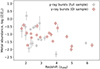 |
Fig. 1. Gas-phase metallicities as a function of redshift. The full GRB sample from Heintz et al. (2023a) is shown by the grey circles with the [O I]-detected subsample highlighted by the red circles. The [O I] sample is representative of the full underlying GRB metallicity-redshift distribution. |
GRB line-of-sight metal abundances and the H I, O I* λ1304 and O I** λ1306 column densities.
The O I-selected bursts probe galaxies spanning redshifts from z = 1.7204 (GRB 191011A) to z = 6.3118 (GRB 210905A). We adopted the H I column densities and dust-corrected metallicities derived by Bolmer et al. (2019), Heintz et al. (2023a) for each burst. The gas-phase metallicities were derived as [X/Y] = log(NX/NH)−log(NX/NH)⊙, with (X/H)⊙ representing solar abundances (Asplund et al. 2021). However, since some of the metals in the interstellar medium are depleted by condensation onto interstellar dust grains, the observed depletion level [X/Y] – which is correlated with the galaxy’s metallicity – was also considered (De Cia et al. 2016). By correcting for the depletion level, an estimate of the total, dust-corrected metallicity [X/H]+[X/Y]=[M/H] was obtained, which is represented as log(Z/Z⊙) (with log(Z/Z⊙) = 0 equivalent to 12 + log(O/H) = 8.69). The GRB sample probes galaxies with H I column densities in the line of sight in excess of NHI = 2 × 1020 cm−2, classifying them as damped Lyman-α absorbers (DLAs; Wolfe et al. 2005). This ensures a large neutrality of the gas due to self-shielding, and is further representative of typical dense, star-forming regions (Jakobsson et al. 2006). The relative metal abundances range from log(Z/Z⊙) = − 2.00 (GRB 140311A) to log(Z/Z⊙) = − 0.29 (GRB 120909A) (that is gas-phase metallicities of 1–50% solar).
2.2. Absorption-line fitting
The procedure used for modelling the absorption line profiles is identical to previous work by Heintz et al. (2018, 2021). In this work, we determined the column densities of the excited fine-structure transitions O I* λ1304 and O I** λ1306 for each GRB in our sample. The absorption line profiles were modelled using VoigtFit (Krogager 2018) which fits a set of Voigt profiles to the observed absorption features and provides the redshift zabs, column density N and broadening parameter b as output. Both O I* and O I** were observed to trace the same neutral interstellar gas components as several other transitions such as Fe II, Si II and C II for the GRB sightlines in our sample. This is further evidence that the excited O I states predominantly traces the neutral gas-phase. We thus used these other transitions to constrain the velocity structure, number of components, and broadening parameters, when fitting the O I* λ1304 and O I** λ1306 line complexes. The intrinsic profiles were first convolved by the measured spectral resolution of each afterglow spectrum. In the case of systems where multiple velocity components were detected, representing individual gas complexes along the line of sight, the sum of the individual column densities was reported. This is consistent with the procedure used to measure the H I abundances and the gas-phase metallicities. An example of the Voigt-profile modelling of the O I* λ1304 and O I** λ1306 transitions in GRB 161023A is shown in Fig. 2. The resulting column densities are listed for the full GRB O I sample in Table 1.
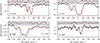 |
Fig. 2. Representative VLT/X-shooter GRB afterglow spectrum of GRB 161023A (de Ugarte Postigo et al. 2018). The observed spectrum is shown in black, the solid red line represents the best-fit model of the marked absorption features. The low-ion Fe II and Si II are used to improve the modelling of the velocity components and line broadening of the O Iλ1302, O I* λ1304 and O I** λ1306 line complexes. |
2.3. Calibrating the [O I]-to-H I conversion factor
The excited fine-structure transitions O I* λ1304 and O I** λ1306 detected in absorption arise from the 3PJ = 1 and 3PJ = 0 levels of neutral atomic oxygen, and were explicitly chosen because they give rise to the far-infrared [O I]−63 μm (3P1 → 3P2) and [O I]−145 μm (3P0 → 3P1) emission line transitions, respectively. This allowed us to derive the corresponding line-of-sight “column” luminosity of [O I]−63 μm and [O I]−145 μm from the spontaneous decay rates, expressed as ![Mathematical equation: $ L^c_{\rm [OI]-63\,\upmu m}=h \nu_{\text{ul}} A_{\text{ul}} N_{\rm OI^*} $](/articles/aa/full_html/2024/05/aa46878-23/aa46878-23-eq3.gif) and likewise for
and likewise for ![Mathematical equation: $ L^c_{\rm [OI]-145\,\upmu m} $](/articles/aa/full_html/2024/05/aa46878-23/aa46878-23-eq4.gif) for each GRB sightline (see also Heintz & Watson 2020; Heintz et al. 2021). Here, h is the Planck constant, νul and Aul are the line frequency and Einstein coefficient, respectively and N is the column density of the excited transition. For [O I]−63 μm, vul = 4744.8 GHz and Aul = 8.91 × 10⁻⁵ s−1 and for [O I]−145 μm, vul = 2060.1 GHz and Aul = 1.75 × 10⁻⁵ s−1. Similarly, the line-of-sight H I mass “colum” density can be determined,
for each GRB sightline (see also Heintz & Watson 2020; Heintz et al. 2021). Here, h is the Planck constant, νul and Aul are the line frequency and Einstein coefficient, respectively and N is the column density of the excited transition. For [O I]−63 μm, vul = 4744.8 GHz and Aul = 8.91 × 10⁻⁵ s−1 and for [O I]−145 μm, vul = 2060.1 GHz and Aul = 1.75 × 10⁻⁵ s−1. Similarly, the line-of-sight H I mass “colum” density can be determined,  , where mHI is the mass of a single hydrogen atom and NHI is the total H I column number density.
For each line of sight, we could thus determine the ratios of the column line luminosities, ![Mathematical equation: $ L^c_{\rm [OI]-63\,\upmu m} $](/articles/aa/full_html/2024/05/aa46878-23/aa46878-23-eq6.gif) and
and ![Mathematical equation: $ L^c_{\rm [OI]-145\,\upmu m} $](/articles/aa/full_html/2024/05/aa46878-23/aa46878-23-eq7.gif) , and relate them to the H I mass column density directly as
, and relate them to the H I mass column density directly as
![Mathematical equation: $$ \begin{aligned} \beta _{\rm [OI]-63\,\upmu m} \equiv \frac{M^c_{\text{HI}}}{L^c_{\rm [OI]-63\,\upmu m}} = \frac{m_{\text{HI}}}{h \nu _{\text{ul}} A_{\text{ul}}} \frac{N_{\text{HI}}}{N_{\rm OI^*}} \end{aligned} $$](/articles/aa/full_html/2024/05/aa46878-23/aa46878-23-eq8.gif) (1)
(1)
and
![Mathematical equation: $$ \begin{aligned} \beta _{\rm [OI]-145\,\upmu m} \equiv \frac{M^c_{\text{HI}}}{L^c_{\rm [OI]-145\,\upmu m}} = \frac{m_{\text{HI}}}{h \nu _{\text{ul}} A_{\text{ul}}} \frac{N_{\text{HI}}}{N_{\rm OI^{**}}}. \end{aligned} $$](/articles/aa/full_html/2024/05/aa46878-23/aa46878-23-eq9.gif) (2)
(2)
These two expressions provide direct [O I]63 μm-to-H I and [O I]145 μm-to-H I conversion factors based on the measured column densities in the line of sight. Assuming that the derived ratios of the column densities for each sightline are representative of the mean of the relative total population that is  . The calibrations derived per unit column are thus equal to the global [O I]63 μm-to-H I and [O I]145 μm-to-H I conversion factors.
This scaling has been derived for both transitions for each GRB in the sample and converted into solar units, M⊙/L⊙, which can simply be expressed as constant factors of the absorption-derived column density ratios as
![Mathematical equation: $$ \begin{aligned} \beta _{\mathrm{[OI]-63\,\upmu m}} = 1.150 \times 10^{-6} \frac{N_{\text{HI}}}{N_{\rm OI^*}} \frac{M_{\odot }}{L_{\odot }} \end{aligned} $$](/articles/aa/full_html/2024/05/aa46878-23/aa46878-23-eq11.gif) (3)
(3)
and
![Mathematical equation: $$ \begin{aligned} \beta _{\rm [OI]-145\,\upmu m} = 1.138 \times 10^{-5} \frac{N_{\text{HI}}}{N_{\rm OI^{**}}} \frac{M_{\odot }}{L_{\odot }}. \end{aligned} $$](/articles/aa/full_html/2024/05/aa46878-23/aa46878-23-eq12.gif) (4)
(4)
We emphasize that this approach only determines the relative mass to luminosity ratios of H I and the two [O I] transitions and not the global properties for the GRB-selected galaxies. These relations thus only provide a conversion between the integrated [O I] luminosities to the total H I gas masses assuming that the GRB sightlines are representative of the overall ISM conditions. As already showcased by Heintz & Watson (2020) using a similar methodology to determine the [C I]-to-H2 calibration and Heintz et al. (2021) for an equivalent [C II]-to-H I calibration, this methodology provides results in remarkable agreement with hydrodynamical simulations of galaxies with similar metallicities (Glover & Smith 2016; Vizgan et al. 2022; Liang et al. 2024), albeit still with the uncertainty on how well the GRB sightlines represent the global properties of the galaxies. Further, the [C II]-to-H I scaling is also reproduced in local galaxies where the H I gas mass can be constrained directly from the 21-cm hyperfine transitions (Rémy-Ruyer et al. 2014; Cormier et al. 2015). This substantiates the assumption that the GRB sightline trace representative regions of the star-forming ISM.
We derived conversion factors in the range log β[OI]−63 μm = −0.389 − 2.205 and log β[OI]−145 μm = 1.561 − 3.589. The full list of measurements for each GRB sightlines is provided in Table 1. As a conservative estimate, we set the systematical uncertainty associated with the column densities for the log β[OI]−63 μm and log β[OI]−145 μm measurements to 0.1 dex and 0.2 dex, respectively, to take into account the uncertainty in the normalization of the spectra and the separation of the absorption-line velocity components. The systematical uncertainty is higher for log β[OI]−145 μm due to the column density of the second excited fine-structure transition often not being as well-constrained. In Sect. 3 we have explored any correlations between the absorption-derived relative abundances of [O I]−63 μm and [O I]−145 μm, and their connection to the metal abundances and absorption-derived [C II]−158 μm luminosities.
3. Results
3.1. The [OI]-63 μm/[OI]-145 μm ratio
Here we first present the ratio of the absorption-derived L[OI]−63 μm and L[OI]−145 μm luminosities (the relative difference in the β[OI]−63 μm and β[OI]−145 μm calibrations) as a function of metallicity and redshift in Fig. 3. We observe a log-linear correlation (albeit less than at the 2σ level) between the absorption-derived L[OI]−63 μm/L[OI]−145 μm ratio and the gas-phase metallicity with the best fit relation log(L[OI]−63 μm/L[OI]−145 μm) = (−0.51 ± 0.26)×log(Z/Z⊙)−(2.15 ± 0.33), and a Pearson correlation coefficient of ρ = 0.435 and a p-value at p = 0.063. There is no apparent physical explanation describing why the metal enrichment of the gas should affect the excitation states of [O I], but it may be driven by the density and temperature of the gas (Kaufman et al. 1999; Hollenbach & Tielens 1999). The L[OI]−63 μm/L[OI]−145 μm ratio is not observed to depend significantly on the redshift (ρ = −0.192 and p = 0.431), which is also indirectly related to the metallicity through the overall chemical evolution of galaxies. We thus simply compute the weighted mean, finding log(L[OI]−63 μm/L[OI]−145 μm) = 1.55 ± 0.12, such that [O I]−63 μm will on average be ≈30× as bright as [O I]−145 μm, at least for galaxies with metallicities of 1 − 50% solar.
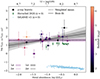 |
Fig. 3. Luminosity ratio for the two selected transitions ([O I]−63 μm and [O I]−145 μm) in log-scale plotted against the metal abundance, log(Z/Z⊙). The black solid line and the grey-shaded regions show the weighted mean of log(L[OI]−63 μm/L[OI]−145 μm) = 1.55 ± 0.12 and the associated 1- and 2-sigma uncertainty. The purple dashed line and the purple-shaded regions show the best fit. The GRBs are color-coded as a function of redshift and are compared to direct measurements from the local z ≈ 0 Herschel Dwarf Galaxy Survey (Madden et al. 2013; Cormier et al. 2015) and to predictions from the SIGAME hydrodynamical simulations framework (Olsen et al. 2021). Overall, the local sample is in good agreement with the GRB observations, whereas the simulation shows a systematical displacement towards a lower luminosity ratio for the two transitions. |
To place our results into context we compare our measurements to a compiled set of local, z ≈ 0 galaxies, with direct measurements of the [O I]-63 μm and [O I]-145 μm line emission from the Herschel Dwarf Galaxy Survey (DGS; Madden et al. 2013) as presented by Cormier et al. (2015) in Fig. 3. All these local galaxies show [O I]-64 μm to [O I]-145 μm line ratios of 10–20, which is significantly lower than our inferred weighted mean (at > 2σ confidence). The oxygen ratios of the two nearby, more massive galaxies M51 (Parkin et al. 2013) and NGC 891 (Hughes et al. 2015) are further consistent with our average estimate, with L[OI]−63 μm/L[OI]−145 μm = 20 ± 9, and = 10.7 ± 3.4, respectively. The dwarf galaxies are arguably more representative of the high-redshift galaxy population due to their lower metallicities and more compact physical sizes.
We also consider the predictions from the Simulator of Galaxy Millimeter/submillimeter Emission (SIGAME) framework (v3; Olsen et al. 2021). This code provides far-infrared line emission estimates calculated through radiative transfer and physically motivated recipes from a particle-based cosmological hydrodynamics simulation (SIMBA; Davé et al. 2019), with this particular version of the code including 400 simulated star-forming galaxies at z ≈ 0. The range of gas densities probed by SIGAME is ≈10−2 − 105 cm−3 and the far-infrared (FIR) lines are modelled using large grid of over 100 000 CLOUDY one-zone models that span the physical conditions (for example density, metallicity, ultraviolet (UV) radiation field, cosmic ray ionisation rate) encountered in the simulations. Comparing these simulations to our results and the compiled sample of local galaxies in Fig. 3 reveal that they substantially underpredict the observed line ratio. This might mainly be due to an incorrect estimate of the excitation of [O I]-63 μm (see also below), limiting the use of these simulations to corroborate our observations at least for the results including the [O I]-63 μm line emission. Indeed, Lupi et al. (2020) finds that inferring [O I] emission line strengths might be particularly model-dependent, as they can be strongly affected by photoionization effects and the thermodynamic state of the gas.
3.2. The [O I]-to-H I conversion factor
Next, we consider the conversion factors log β[OI]−63 μm and log β[OI]−145 μm, shown in Fig. 4 as a function of gas-phase metallicity. We observe a significant log-linear anti-correlation of log β[OI]−63 μm with the metallicity, with a Pearson correlation coefficient of ρ = −0.561 and a p-value at p = 0.012. Similarly for log β[OI]−145 μm, there appears to be a mild log-linear anti-correlation, with a Pearson correlation coefficient of ρ = −0.258 and a p-value at p = 0.287. We derive best-fit [O I]-to-H I scaling relations of
![Mathematical equation: $$ \begin{aligned}&\log (M_{\text{HI}}/M_\odot ) = (-0.77 \pm 0.14) \times \log (Z/Z_{\odot }) \nonumber \\&\qquad \qquad \qquad - (0.26 \pm 0.18) + \log (L_{\rm [OI]-63\,\upmu m}/L_\odot ) \end{aligned} $$](/articles/aa/full_html/2024/05/aa46878-23/aa46878-23-eq13.gif) (5)
(5)
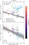 |
Fig. 4. Absorption-derived [O I]63 μm-to-H I (top panel) and [O I]145 μm-to-H I (bottom panel) conversion factors as a function of metallicity. The color and symbol notation follow Fig. 3. The black solid line and the grey-shaded region in the top panel represents the best fit linear relation and the associated uncertainty. The dotted line in the bottom panel shows the best fit of the intersection with the slope fixed at the value of the slope from the fit in the top panel. The dashed line consist of the fit from the top panel with the weighted mean added. The grey-shaded region includes the uncertainties associated with the fit from the top panel as well as the weighted mean. The local samples are shown as upper limits and are in fine agreement with the absorption-derived conversion factors for both transitions in the GRB observations. The simulation is in good agreement with the [O I]145 μm-to-H I conversion factor, while there seems to be a systematical displacement towards higher values for the [O I]63 μm-to-H I conversion factor. |
and
![Mathematical equation: $$ \begin{aligned}&\log (M_{\text{HI}}/M_\odot ) = (-0.77\pm 0.18) \times \log (Z/Z_{\odot }) \nonumber \\&\qquad \qquad + (1.40 \pm 0.22) + \log (L_{\rm [OI]-145\,\upmu m}/L_\odot ). \end{aligned} $$](/articles/aa/full_html/2024/05/aa46878-23/aa46878-23-eq14.gif) (6)
(6)
In Eq. (6), we have fixed the slope in the [O I]145 μm-to-H I scaling relation to the slope found from the best-fit of [O I]63 μm-to-H I scaling relation (Eq. (5)) and instead only fitted the intercept. This is mostly motivated by the significantly larger scatter of the log β[OI]−145 μm measurements due to the more uncertain column density measurements of O I** λ1306, and the fact that the [O I]145 μm to [O I]63 μm ratio is theoretically expected to be constant. The larger scatter of the O I** λ1306 measurements, however, is included in this prescription, and shown by the grey-shaded area in Fig. 4.
We again compare our observations to the Herschel DGS, including the H I gas mass and [O I] emission measurements from Rémy-Ruyer et al. (2014), Cormier et al. (2015), and now also including the LITTLE THINGS dwarf galaxy sample with measurements of [O I]-63 μ and MHI as well (Cigan et al. 2016). The galaxies from the DGS and LITTLE THINGS at z ≈ 0 appear to have systematically higher [O I]145 μm-to-H I abundance ratios at > 3σ than observed in the GRB sightlines at z > 2. This could indicate that high-redshift galaxies potentially have less abundant H I gas reservoirs per O I abundance or, conversely, that their [O I] emission are brighter on average. More likely, is it that the local galaxy observations probe more diffuse, extended H I gas via the 21-cm transition than recovered by the high-redshift FIR lines (see e.g., Heintz et al. 2023b). We therefore represent the derived [O I]-to-H I ratios for the local galaxy samples as upper limits galaxies in Fig. 4. Comparing our observations to the SIGAME simulations yields a good agreement between the observed and predicted [O I]145 μm-to-H I relation. The predictions for the [O I]63 μm-to-H I ratio from SIGAME, however, are generally overestimated compared to our observations, which may indicate that the [O I]63 μm emission line strength is underestimated in these simulations and thereby also causing the inferred low [O I]-63 μm/[oi]-145 μm ratio.
3.3. The [C II]/[O I] ratio
Finally, in Fig. 5 we show the absorption-derived [C II]-158 μm to the [O I]-63 μm and [O I]-145 μm luminosity ratios as a function of metallicity, respectively. For this, we primarily adopt the C II* λ1335.7 measurements from Heintz et al. (2021), but also derive additional C II* λ1335.7 abundances for GRBs 181020A, 190106A, 190114A, 191011A and 210905A following the same approach outlined in Sect. 2.2 (see Table 1). We do not observe any strong correlation for L[CII]−158 μm/L[OI]−145 μm as a function of metallicity, with Pearson correlation coefficient of ρ = −0.063 and p-value p = 0.804. For L[CII]−158 μm/L[OI]−63 μm as a function of metallicity the correlation is on the contrary significant with Pearson correlation coefficient of ρ = 0.407 and p-value p = 0.094. An overview of all Pearson correlations and p-values mentioned throughout this section can be seen in Table 2. For both L[CII]−158 μm/L[OI]−145 μm and L[CII]−158 μm/L[OI]−63 μm vs. metallicity we compute weighted means of −1.91 ± 0.07 and −0.27 ± 0.09, respectively. These results indicate that the gas probed by the GRB sightlines generally predict weaker [C II]-158 μm emission than either of the two far-infrared [O I] transitions.
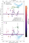 |
Fig. 5. Absorption-derived [O I]63 μm-to-[C II]158 μm and [O I]145 μm-to-[C II]158 μm line luminosity ratios as a function of metallicity and redshift. The color and symbol notation follow Fig. 3. The black solid lines and the grey-shaded regions show the weighted means and the associated 1- and 2-sigma uncertainty of each line ratio. Similar to Fig. 4 the local samples are shown as upper limits and are in fine agreement with the absorption-derived line luminosity ratios for both transitions in the GRB observations. Similarly to the absorption-derived [O I]63 μm-to-H I conversion factor, the simulation suggests a systematical displacement in the absorption-derived [O I]63 μm-to-[C II]158 μm line luminosity. |
Pearson correlation coefficients and p-values.
Comparing our observations again to the simulations and local galaxy samples mentioned in the previous sections, we find that the GRBs generally probe lower line ratios L[CII]−158 μm/L[OI]−63 μm. While the same is true for L[CII]−158 μm/L[OI]−145 μm for the local galaxy vs. GRB sample, we observe that the SIGAME simulations are in better agreement with our observations (similar to the [O I]-to-H I ratio). This might suggest that the GRB sightlines generally probe warmer and much denser gas in the ISM of their host galaxies, compared to the ISM gas in local galaxies (see e.g., Popping et al. 2014; De Breuck et al. 2019).
4. Application to [O I]-emitting galaxies at high redshifts
In an attempt to enable estimates of the H I gas masses of high-redshift galaxies, we have derived the [O I]63 μm-to-H I and [O I]145 μm-to-H I conversion factors as a function of gas-phase metallicity in star-forming galaxies at z ≈ 2 − 6 using GRBs as probes. The conversion factors derived here are observed either in absorption or directly in emission from the ISM of “normal” main-sequence star-forming galaxies, albeit over a large span in redshift and metallicity. These scaling relations are therefore only applicable to sources with similar ISM properties. We consider the main-sequence galaxies at z ≈ 1.5 from Wagg et al. (2020), who presents a single [O I]-63 μm line detection for the galaxy BzK-21000 at z = 1.5213 with a luminosity of L[OI]−63 μm = (3.9 ± 0.7)×109 L⊙. While [O I] is not detected in the remaining spectra, their stacking analysis reveals L[OI]−63 μm = (1.1 ± 0.2)×109 L⊙. Since their targets all have stellar masses, M⋆ ≳ 1010.5 M⊙, we assume solar metallicities and infer from Eq. (6) H I gas masses of MHI ≈ 5 × 10⁸ − 2 × 10⁹. These results imply low H I gas fractions of MHI/M⋆ ≈ 2 − 6% for the star-forming galaxies at z ≈ 1.5.
In the near future we are likely to expect an increasing number of [O I] detections from “regular” star-forming galaxies at greater redshifts. In particular, the [O I]-63 μm transition will be redshifted into the ALMA band 9 and the [O I]-145 μm transition will be placed in band 7 at z ≳ 6, enabling measurements of these important neutral gas tracers with few hours of on-target integration for the brightest [O I]-emitting sources in the epoch of reionization (as also proposed by Lupi et al. 2020; Pallottini et al. 2022). To fully optimize the use of the derived [O I]63 μm-to-H I and [O I]145 μm-to-H I gas tracers, complementary JWST observations are needed to provide constraints on the metallicity of the sources at z > 6 (see e.g., Heintz et al. 2023b).
5. Conclusions
In this work we presented the first high-redshift calibrations of the [O I]63 μm-to-H I and [O I]145 μm-to-H I conversion factors, here denoted β[OI]−63 μm and β[OI]−145 μm, respectively. This work was made in continuation of recent attempts to establish a similar [C II]-to-H I calibration (e.g., Heintz et al. 2021, 2022). Due to the weakness of the direct 21-cm H I gas tracers, such calibrations are the only alternative, and therefore vital, to infer the neutral atomic gas content of the most distant galaxies. While the far-infrared [C II]-158 μm transition is typically the brightest of the ISM cooling lines, this feature can originate from both neutral and ionized gas, making it a less optimal tracer of the neutral atomic gas only. The ionization potential and critical density of [O I] on the other hand, ensures that the far-infrared [O I]-63 μm and [O I]-145 μm transitions predominantly originates from the neutral ISM (Hollenbach & Tielens 1999).
We calibrate the β[OI]−63 μm and β[OI]−145 μm conversion factors using GRBs as probes of the dense, star-forming ISM in their host galaxies, spanning redshifts z = 1.7 − 6.3 and gas-phase metallicities from 1–50% solar. We derive the calibrations from the measured column densities of the excited O I* λ1304 and O I** λ1306 transitions detected in absorption, which give rise to the far-infrared [O I]-63 μm and [O I]-145 μm emission lines, and from Lyman-α for H I. The excited O I transitions provide a measure of the luminosity per unit column assuming spontaneous decay, and Lyman-α the H I mass per unit column. We found that both [O I]-to-H I conversion factors are anti-correlated with the gas-phase metallicity, with best-fit scaling relations given in Eqs. (5) and (6). These indicate that galaxies with 10% solar metallicities have approx. ×10 higher H I gas masses for a given [O I] line luminosity compared to galaxies at solar metallicities.
We further made predictions for the line luminosity ratios of [O I]-63 μm, [O I]-145 μm, and [C II]-158 μm based on the absorption-derived conversion factors, for which we derived weighted means of log(L[OI]−63 μm/L[OI]−145 μm) = 1.55 ± 0.12, log(L[CII]−158 μm/L[OI]−63 μm) = −1.91 ± 0.07, and log(L[CII]−158 μm/L[OI]−145 μm) = −0.27 ± 0.09. Overall, these results indicate that the [O I] transitions might be the brightest far-infrared ISM cooling lines at high redshifts. We further compared our measurements with hydrodynamical simulations from the SIGAME framework and local galaxy samples (Madden et al. 2013; Parkin et al. 2013; Hughes et al. 2015; Cigan et al. 2016) for which the H I gas mass could be measured directly through the 21-cm line emission. The predicted [O I]145 μm-to-H I ratio from the simulations were found to be statistically consistent with our results, whereas the simulated [O I]63 μm-to-H I ratios showed significant offset (at > 3σ) towards higher ratios than our inferred relation. The compiled local Herschel dwarf galaxy sample at z ≈ 0 (Madden et al. 2013; Rémy-Ruyer et al. 2014; Cormier et al. 2015), generally showed suppressed [O I] emission for both transitions at any given H I gas mass and metallicity, which we surmised could be related to the typical lower volumetric hydrogen gas densities of low-redshift galaxies, or conversely more extended, diffuse H I gas components traced by the 21-cm line.
While the next generation radio detection facilities such as the Square Kilometre Array (SKA) will significantly improve the sensitivity and the redshift range for which the H I 21-cm line transition can be detected directly, these measurements will still be limited to the most massive galaxies and out to moderate distances only at z ≈ 1.7 (Blyth et al. 2015). Inferring the neutral gas content of the most distant galaxies thus necessitates the development and use of alternative gas tracers. We encourage further simulations and empirical observations to substantiate the high-redshift [O I]-to-H I calibrations derived here to establish a new window into the build-up of neutral gas in the star-forming of ISM galaxies in the early universe.
Acknowledgments
K.E.H. acknowledges support from the Carlsberg Foundation Reintegration Fellowship Grant CF21-0103. The Cosmic Dawn Center (DAWN) is funded by the Danish National Research Foundation under grant No. 140. This work is partly based on observations collected at the European Organisation for Astronomical Research in the Southern Hemisphere.
References
- Asplund, M., Amarsi, A. M., & Grevesse, N. 2021, A&A, 653, A141 [NASA ADS] [CrossRef] [EDP Sciences] [Google Scholar]
- Blyth, S., van der Hulst, T. M., Verheijen, M. A. W., et al. 2015, in Advancing Astrophysics with the Square Kilometre Array (AASKA14), 128 [CrossRef] [Google Scholar]
- Bolatto, A. D., Wolfire, M., & Leroy, A. K. 2013, ARA&A, 51, 207 [CrossRef] [Google Scholar]
- Bolmer, J., Ledoux, C., Wiseman, P., et al. 2019, A&A, 623, A43 [NASA ADS] [CrossRef] [EDP Sciences] [Google Scholar]
- Bouwens, R. J., Smit, R., Schouws, S., et al. 2022, ApJ, 931, 160 [NASA ADS] [CrossRef] [Google Scholar]
- Brisbin, D., Ferkinhoff, C., Nikola, T., et al. 2015, ApJ, 799, 13 [Google Scholar]
- Cano, Z., Wang, S.-Q., Dai, Z.-G., & Wu, X.-F. 2017, Adv. Astron., 2017, 8929054a [CrossRef] [Google Scholar]
- Carilli, C. L., & Walter, F. 2013, ARA&A, 51, 105 [NASA ADS] [CrossRef] [Google Scholar]
- Catinella, B., Saintonge, A., Janowiecki, S., et al. 2018, MNRAS, 476, 875 [NASA ADS] [CrossRef] [Google Scholar]
- Chakraborty, A., & Roy, N. 2023, MNRAS, 519, 4074 [NASA ADS] [CrossRef] [Google Scholar]
- Chowdhury, A., Kanekar, N., Chengalur, J. N., Sethi, S., & Dwarakanath, K. S. 2020, Nature, 586, 369 [Google Scholar]
- Cigan, P., Young, L., Cormier, D., et al. 2016, AJ, 151, 14 [NASA ADS] [CrossRef] [Google Scholar]
- Coppin, K. E. K., Danielson, A. L. R., Geach, J. E., et al. 2012, MNRAS, 427, 520 [NASA ADS] [CrossRef] [Google Scholar]
- Cormier, D., Madden, S. C., Lebouteiller, V., et al. 2015, A&A, 578, A53 [CrossRef] [EDP Sciences] [Google Scholar]
- Cormier, D., Abel, N. P., Hony, S., et al. 2019, A&A, 626, A23 [NASA ADS] [CrossRef] [EDP Sciences] [Google Scholar]
- Crocker, A. F., Pellegrini, E., Smith, J. D. T., et al. 2019, ApJ, 887, 105 [NASA ADS] [CrossRef] [Google Scholar]
- Croxall, K. V., Smith, J. D., Pellegrini, E., et al. 2017, ApJ, 845, 96 [Google Scholar]
- Davé, R., Anglés-Alcázar, D., Narayanan, D., et al. 2019, MNRAS, 486, 2827 [Google Scholar]
- Dayal, P., & Ferrara, A. 2018, Phys. Rep., 780, 1 [Google Scholar]
- De Breuck, C., WeiSS, A., Béthermin, M., et al. 2019, A&A, 631, A167 [NASA ADS] [CrossRef] [EDP Sciences] [Google Scholar]
- De Cia, A., Ledoux, C., Mattsson, L., et al. 2016, A&A, 596, A97 [NASA ADS] [CrossRef] [EDP Sciences] [Google Scholar]
- de Ugarte Postigo, A., Thöne, C. C., Bolmer, J., et al. 2018, A&A, 620, A119 [NASA ADS] [CrossRef] [EDP Sciences] [Google Scholar]
- Fernández, X., Gim, H. B., van Gorkom, J. H., et al. 2016, ApJ, 824, L1 [Google Scholar]
- Ferrara, A., Vallini, L., Pallottini, A., et al. 2019, MNRAS, 489, 1 [Google Scholar]
- Franeck, A., Walch, S., Seifried, D., et al. 2018, MNRAS, 481, 4277 [NASA ADS] [CrossRef] [Google Scholar]
- Fujimoto, S., Ouchi, M., Nakajima, K., et al. 2024, ApJ, 964, 146 [NASA ADS] [CrossRef] [Google Scholar]
- Fynbo, J. P. U., Starling, R. L. C., Ledoux, C., et al. 2006, A&A, 451, L47 [NASA ADS] [CrossRef] [EDP Sciences] [Google Scholar]
- Gehrels, N., Ramirez-Ruiz, E., & Fox, D. B. 2009, ARA&A, 47, 567 [NASA ADS] [CrossRef] [Google Scholar]
- Genzel, R., Tacconi, L. J., Lutz, D., et al. 2015, ApJ, 800, 20 [Google Scholar]
- Glover, S. C. O., & Smith, R. J. 2016, MNRAS, 462, 3011 [NASA ADS] [CrossRef] [Google Scholar]
- Hartoog, O. E., Malesani, D., Fynbo, J. P. U., et al. 2015, A&A, 580, A139 [NASA ADS] [CrossRef] [EDP Sciences] [Google Scholar]
- Heintz, K. E., & Watson, D. 2020, ApJ, 889, L7 [Google Scholar]
- Heintz, K. E., Watson, D., Jakobsson, P., et al. 2018, MNRAS, 479, 3456 [Google Scholar]
- Heintz, K. E., Watson, D., Oesch, P. A., Narayanan, D., & Madden, S. C. 2021, ApJ, 922, 147 [NASA ADS] [CrossRef] [Google Scholar]
- Heintz, K. E., Oesch, P. A., Aravena, M., et al. 2022, ApJ, 934, L27 [NASA ADS] [CrossRef] [Google Scholar]
- Heintz, K. E., De Cia, A., Thöne, C. C., et al. 2023a, A&A, 679, A91 [NASA ADS] [CrossRef] [EDP Sciences] [Google Scholar]
- Heintz, K. E., Giménez-Arteaga, C., Fujimoto, S., et al. 2023b, ApJ, 944, L30 [NASA ADS] [CrossRef] [Google Scholar]
- Heintz, K. E., Watson, D., Brammer, G., et al. 2023c, arXiv e-prints [arXiv:2306.00647] [Google Scholar]
- Hollenbach, D. J., & Tielens, A. G. G. M. 1999, Rev. Mod. Phys., 71, 173 [Google Scholar]
- Hoppmann, L., Staveley-Smith, L., Freudling, W., et al. 2015, MNRAS, 452, 3726 [NASA ADS] [CrossRef] [Google Scholar]
- Hughes, T. M., Foyle, K., Schirm, M. R. P., et al. 2015, A&A, 575, A17 [NASA ADS] [CrossRef] [EDP Sciences] [Google Scholar]
- Jakobsson, P., Hjorth, J., Fynbo, J. P. U., et al. 2004, A&A, 427, 785 [NASA ADS] [CrossRef] [EDP Sciences] [Google Scholar]
- Jakobsson, P., Fynbo, J. P. U., Ledoux, C., et al. 2006, A&A, 460, L13 [NASA ADS] [CrossRef] [EDP Sciences] [Google Scholar]
- Jones, M. G., Haynes, M. P., Giovanelli, R., & Moorman, C. 2018, MNRAS, 477, 2 [Google Scholar]
- Kaufman, M. J., Wolfire, M. G., Hollenbach, D. J., & Luhman, M. L. 1999, ApJ, 527, 795 [Google Scholar]
- Kereš, D., Katz, N., Weinberg, D. H., & Davé, R. 2005, MNRAS, 363, 2 [Google Scholar]
- Krogager, J. K. 2018, arXiv e-prints [arXiv:1803.01187] [Google Scholar]
- Lagache, G., Cousin, M., & Chatzikos, M. 2018, A&A, 609, A130 [NASA ADS] [CrossRef] [EDP Sciences] [Google Scholar]
- Liang, L., Feldmann, R., Murray, N., et al. 2024, MNRAS, 528, 499 [NASA ADS] [CrossRef] [Google Scholar]
- Lodders, K., Palme, H., & Gail, H. P. 2009, Landolt Börnstein, 4B, 712 [Google Scholar]
- Lupi, A., Pallottini, A., Ferrara, A., et al. 2020, MNRAS, 496, 5160 [Google Scholar]
- Madden, S. C., Geis, N., Genzel, R., et al. 1993, ApJ, 407, 579 [NASA ADS] [CrossRef] [Google Scholar]
- Madden, S. C., Poglitsch, A., Geis, N., Stacey, G. J., & Townes, C. H. 1997, ApJ, 483, 200 [NASA ADS] [CrossRef] [Google Scholar]
- Madden, S. C., Rémy-Ruyer, A., Galametz, M., et al. 2013, PASP, 125, 600 [NASA ADS] [CrossRef] [Google Scholar]
- Maddox, N., Frank, B. S., Ponomareva, A. A., et al. 2021, A&A, 646, A35 [NASA ADS] [CrossRef] [EDP Sciences] [Google Scholar]
- Magdis, G. E., Daddi, E., Béthermin, M., et al. 2012, ApJ, 760, 6 [NASA ADS] [CrossRef] [Google Scholar]
- Meyer, R. A., Walter, F., Cicone, C., et al. 2022, ApJ, 927, 152 [NASA ADS] [CrossRef] [Google Scholar]
- Narayanan, D., & Krumholz, M. R. 2017, MNRAS, 467, 50 [NASA ADS] [CrossRef] [Google Scholar]
- Olsen, K. P., Burkhart, B., Mac Low, M.-M., et al. 2021, ApJ, 922, 88 [NASA ADS] [CrossRef] [Google Scholar]
- Pallottini, A., Ferrara, A., Bovino, S., et al. 2017, MNRAS, 471, 4128 [NASA ADS] [CrossRef] [Google Scholar]
- Pallottini, A., Ferrara, A., Gallerani, S., et al. 2022, MNRAS, 513, 5621 [NASA ADS] [Google Scholar]
- Parkin, T. J., Wilson, C. D., Schirm, M. R. P., et al. 2013, ApJ, 776, 65 [Google Scholar]
- Pineda, J. L., Langer, W. D., & Goldsmith, P. F. 2014, A&A, 570, A121 [NASA ADS] [CrossRef] [EDP Sciences] [Google Scholar]
- Planck Collaboration VI. 2020, A&A, 641, A6 [NASA ADS] [CrossRef] [EDP Sciences] [Google Scholar]
- Popping, G., Pérez-Beaupuits, J. P., Spaans, M., Trager, S. C., & Somerville, R. S. 2014, MNRAS, 444, 1301 [NASA ADS] [CrossRef] [Google Scholar]
- Popping, G., Narayanan, D., Somerville, R. S., Faisst, A. L., & Krumholz, M. R. 2019, MNRAS, 482, 4906 [Google Scholar]
- Popping, G., van Kampen, E., Decarli, R., et al. 2016, MNRAS, 461, 93 [NASA ADS] [CrossRef] [Google Scholar]
- Prochaska, J. X., Chen, H.-W., Dessauges-Zavadsky, M., & Bloom, J. S. 2007, ApJ, 666, 267 [NASA ADS] [CrossRef] [Google Scholar]
- Ramos Padilla, A. F., Wang, L., Ploeckinger, S., van der Tak, F. F. S., & Trager, S. C. 2021, A&A, 645, A133 [NASA ADS] [CrossRef] [EDP Sciences] [Google Scholar]
- Rémy-Ruyer, A., Madden, S. C., Galliano, F., et al. 2014, A&A, 563, A31 [Google Scholar]
- Robertson, B. E., & Ellis, R. S. 2012, ApJ, 744, 95 [Google Scholar]
- Rybak, M., Zavala, J. A., Hodge, J. A., Casey, C. M., & Werf, P. v. d. 2020, ApJ, 889, L11 [NASA ADS] [CrossRef] [Google Scholar]
- Saccardi, A., Vergani, S. D., De Cia, A., et al. 2023, A&A, 671, A84 [NASA ADS] [CrossRef] [EDP Sciences] [Google Scholar]
- Schaye, J., Dalla Vecchia, C., Booth, C. M., et al. 2010, MNRAS, 402, 1536 [Google Scholar]
- Selsing, J., Malesani, D., Goldoni, P., et al. 2019, A&A, 623, A92 [NASA ADS] [CrossRef] [EDP Sciences] [Google Scholar]
- Smit, R., Bouwens, R. J., Carniani, S., et al. 2018, Nature, 553, 178 [Google Scholar]
- Tacconi, L. J., Genzel, R., Neri, R., et al. 2010, Nature, 463, 781 [Google Scholar]
- Tacconi, L. J., Neri, R., Genzel, R., et al. 2013, ApJ, 768, 74 [NASA ADS] [CrossRef] [Google Scholar]
- Tarantino, E., Bolatto, A. D., Herrera-Camus, R., et al. 2021, ApJ, 915, 92 [NASA ADS] [CrossRef] [Google Scholar]
- Valentino, F., Magdis, G. E., Daddi, E., et al. 2018, ApJ, 869, 27 [Google Scholar]
- Vallini, L., Gallerani, S., Ferrara, A., Pallottini, A., & Yue, B. 2015, ApJ, 813, 36 [NASA ADS] [CrossRef] [Google Scholar]
- Vallini, L., Ferrara, A., Pallottini, A., & Gallerani, S. 2017, MNRAS, 467, 1300 [NASA ADS] [Google Scholar]
- Vizgan, D., Heintz, K. E., Greve, T. R., et al. 2022, ApJ, 939, L1 [NASA ADS] [CrossRef] [Google Scholar]
- Wagg, J., Aravena, M., Brisbin, D., et al. 2020, MNRAS, 499, 1788 [NASA ADS] [CrossRef] [Google Scholar]
- Walter, F., Brinks, E., de Blok, W. J. G., et al. 2008, AJ, 136, 2563 [Google Scholar]
- Walter, F., Weiß, A., Downes, D., Decarli, R., & Henkel, C. 2011, ApJ, 730, 18 [Google Scholar]
- Wardlow, J. L., Cooray, A., Osage, W., et al. 2017, ApJ, 837, 12 [NASA ADS] [CrossRef] [Google Scholar]
- Weiß, A., Henkel, C., Downes, D., & Walter, F. 2003, A&A, 409, L41 [NASA ADS] [CrossRef] [EDP Sciences] [Google Scholar]
- Wolfe, A. M., Gawiser, E., & Prochaska, J. X. 2005, ARA&A, 43, 861 [NASA ADS] [CrossRef] [Google Scholar]
- Wolfire, M. G., Vallini, L., & Chevance, M. 2022, ARA&A, 60, 247 [NASA ADS] [CrossRef] [Google Scholar]
- Woosley, S. E., & Bloom, J. S. 2006, ARA&A, 44, 507 [Google Scholar]
- Yoon, S. C., Langer, N., & Norman, C. 2006, A&A, 460, 199 [NASA ADS] [CrossRef] [EDP Sciences] [Google Scholar]
- Zwaan, M. A., Meyer, M. J., Staveley-Smith, L., & Webster, R. L. 2005, MNRAS, 359, L30 [NASA ADS] [CrossRef] [Google Scholar]
All Tables
GRB line-of-sight metal abundances and the H I, O I* λ1304 and O I** λ1306 column densities.
All Figures
|
Fig. 1. Gas-phase metallicities as a function of redshift. The full GRB sample from Heintz et al. (2023a) is shown by the grey circles with the [O I]-detected subsample highlighted by the red circles. The [O I] sample is representative of the full underlying GRB metallicity-redshift distribution. |
| In the text | |
|
Fig. 2. Representative VLT/X-shooter GRB afterglow spectrum of GRB 161023A (de Ugarte Postigo et al. 2018). The observed spectrum is shown in black, the solid red line represents the best-fit model of the marked absorption features. The low-ion Fe II and Si II are used to improve the modelling of the velocity components and line broadening of the O Iλ1302, O I* λ1304 and O I** λ1306 line complexes. |
| In the text | |
|
Fig. 3. Luminosity ratio for the two selected transitions ([O I]−63 μm and [O I]−145 μm) in log-scale plotted against the metal abundance, log(Z/Z⊙). The black solid line and the grey-shaded regions show the weighted mean of log(L[OI]−63 μm/L[OI]−145 μm) = 1.55 ± 0.12 and the associated 1- and 2-sigma uncertainty. The purple dashed line and the purple-shaded regions show the best fit. The GRBs are color-coded as a function of redshift and are compared to direct measurements from the local z ≈ 0 Herschel Dwarf Galaxy Survey (Madden et al. 2013; Cormier et al. 2015) and to predictions from the SIGAME hydrodynamical simulations framework (Olsen et al. 2021). Overall, the local sample is in good agreement with the GRB observations, whereas the simulation shows a systematical displacement towards a lower luminosity ratio for the two transitions. |
| In the text | |
|
Fig. 4. Absorption-derived [O I]63 μm-to-H I (top panel) and [O I]145 μm-to-H I (bottom panel) conversion factors as a function of metallicity. The color and symbol notation follow Fig. 3. The black solid line and the grey-shaded region in the top panel represents the best fit linear relation and the associated uncertainty. The dotted line in the bottom panel shows the best fit of the intersection with the slope fixed at the value of the slope from the fit in the top panel. The dashed line consist of the fit from the top panel with the weighted mean added. The grey-shaded region includes the uncertainties associated with the fit from the top panel as well as the weighted mean. The local samples are shown as upper limits and are in fine agreement with the absorption-derived conversion factors for both transitions in the GRB observations. The simulation is in good agreement with the [O I]145 μm-to-H I conversion factor, while there seems to be a systematical displacement towards higher values for the [O I]63 μm-to-H I conversion factor. |
| In the text | |
|
Fig. 5. Absorption-derived [O I]63 μm-to-[C II]158 μm and [O I]145 μm-to-[C II]158 μm line luminosity ratios as a function of metallicity and redshift. The color and symbol notation follow Fig. 3. The black solid lines and the grey-shaded regions show the weighted means and the associated 1- and 2-sigma uncertainty of each line ratio. Similar to Fig. 4 the local samples are shown as upper limits and are in fine agreement with the absorption-derived line luminosity ratios for both transitions in the GRB observations. Similarly to the absorption-derived [O I]63 μm-to-H I conversion factor, the simulation suggests a systematical displacement in the absorption-derived [O I]63 μm-to-[C II]158 μm line luminosity. |
| In the text | |
Current usage metrics show cumulative count of Article Views (full-text article views including HTML views, PDF and ePub downloads, according to the available data) and Abstracts Views on Vision4Press platform.
Data correspond to usage on the plateform after 2015. The current usage metrics is available 48-96 hours after online publication and is updated daily on week days.
Initial download of the metrics may take a while.