| Issue |
A&A
Volume 678, October 2023
|
|
|---|---|---|
| Article Number | A30 | |
| Number of page(s) | 7 | |
| Section | Extragalactic astronomy | |
| DOI | https://doi.org/10.1051/0004-6361/202346573 | |
| Published online | 28 September 2023 | |
Gauging the mass of metals in the gas phase of galaxies from the Local Universe to the Epoch of Reionization
1
Cosmic Dawn Center (DAWN), Denmark
2
Niels Bohr Institute, University of Copenhagen, Jagtvej 128, 2200 Copenhagen N, Denmark
e-mail: This email address is being protected from spambots. You need JavaScript enabled to view it.
3
Department of Physics and Astronomy, University of California, Los Angeles, 430 Portola Plaza, Los Angeles, CA 90095, USA
4
Department of Physics, University of California, Davis, 1 Shields Avenue, Davis, CA 95616, USA
5
DTU-Space, Technical University of Denmark, Elektrovej 327, 2800 Kgs. Lyngby, Denmark
6
Dipartimento di Fisica e Astronomia, Università di Firenze, Via G. Sansone 1, 50019 Sesto Fiorentino, Firenze, Italy
7
Department of Astronomy, University of Florida, Gainesville, FL 32611, USA
8
Department of Astronomy, University of Illinois at Urbana-Champaign, 1002 West Green St., Urbana, IL 61801, USA
Received:
2
April
2023
Accepted:
30
July
2023
Abstract
The chemical enrichment of dust and metals are vital processes in constraining the star formation history of the universe. These are important ingredients in the formation and evolution of galaxies overall. Previously, the dust masses of high-redshift star-forming galaxies have been determined through their far-infrared continuum, however, equivalent, and potentially simpler, approaches to determining the metal masses have yet to be explored at z ≳ 2. Here, we present a new method of inferring the metal mass in the interstellar medium (ISM) of galaxies out to z ≈ 8, using the far-infrared [C II]−158 μm emission line as a proxy. We calibrated the [C II]-to-MZ, ISM conversion factor based on a benchmark observational sample at z ≈ 0, in addition to gamma-ray burst sightlines at z > 2 and cosmological hydrodynamical simulations of galaxies at z ≈ 0 and z ≈ 6. We found a universal scaling across redshifts of log(MZ, ISM/M⊙) = log(L[CII]/L⊙)−0.45, with a 0.4 dex scatter, which is constant over more than two orders of magnitude in metallicity. We applied this scaling to recent surveys for [C II] in galaxies at z ≳ 2 and compared their inferred MZ, ISM to their stellar mass (M⋆). In particular, we determined the fraction of metals retained in the gas-phase ISM, MZ, ISM/M⋆, as a function of redshift and we showed that an increasing fraction of metals reside in the ISM of galaxies at higher redshifts. We place further constraints on the cosmic metal mass density in the ISM (ΩZ, ISM) at z ≈ 5 and ≈7 based on recent estimates of the [C II]−158 μm luminosity functions at these epochs, yielding ΩZ,ISM = 6.6−4.3+13 × 10−7 M⊙ Mpc−3 (z ≈ 5) and ΩZ,ISM = 2.0−1.3+3.5 × 10⁻⁷ M⊙ Mpc−3 (z ≈ 7), respectively. These results are consistent with the expected metal yields from the integrated star formation history at the respective redshifts. This suggests that the majority of metals produced at z ≳ 5 are confined to the ISM, with strong implications that disfavor efficient outflow processes at these redshifts. Instead, these results suggest that the extended [C II] halos predominantly trace the extended neutral gas reservoirs of high-z galaxies.
Key words: galaxies: evolution / galaxies: high-redshift / galaxies: ISM / galaxies: star formation
© The Authors 2023
 Open Access article, published by EDP Sciences, under the terms of the Creative Commons Attribution License (https://creativecommons.org/licenses/by/4.0), which permits unrestricted use, distribution, and reproduction in any medium, provided the original work is properly cited.
This article is published in open access under the Subscribe to Open model. This email address is being protected from spambots. You need JavaScript enabled to view it. to support open access publication.
1. Introduction
The metal enrichment of the interstellar medium (ISM) of a galaxy is an imprint left behind by stellar processing. It encodes information about the star formation history (SFH) of the galaxy and simultaneously provides insight into the complex processes that regulate the metal content, such as large-scale gas infall and outflows (Heintz et al. 2022a). Similarly, the amount of dust directly informs the dust yields from the explosions of core-collapse supernovae (e.g., Gall et al. 2014; Leśniewska & Michałowski 2019) and the efficiency of metals depleting into dust grains through ISM growth (e.g., Dwek 1998). Therefore, obtaining a complete census of the dust and metals in galaxies, particularly at the earliest epochs, is vital to constraining these processes and understanding the formation and evolution of the first generation of galaxies overall.
Early attempts to gauge the metal census at high redshift reported that the bulk of the expected metals from the integrated SFH at z ≈ 2 were missing from the ISM, having likely been expelled through outflows (Pettini et al. 1999; Prochaska et al. 2003; Ferrara et al. 2005; Bouché et al. 2007). This led to the long-standing “missing metals problem”, of which only 30% to 90% of the expected cosmic density of metals could be accounted for in the intergalactic medium (IGM), the ISM, and in stars (Ferrara et al. 2005; Bouché et al. 2007). However, these early studies were significantly affected by biased selections of quasars and, as a consequence, they were unable to identify the most metal- and dust-rich foreground absorbers (e.g., Fall & Pei 1993; Heintz et al. 2018; Krogager et al. 2019). Accounting for this bias and the total amount of metals locked into dust grains has yielded cosmic metal mass densities in the ISM of galaxies at z ≳ 2.5, which is consistent with the total integrated SFH metal yield (Péroux & Howk 2020). Yet even this approach is limited in the sense that quasar absorbers are increasingly less robust tracers of the ISM in galaxies at higher redshifts, mainly probing the diffuse circumgalactic medium in the outskirts of their absorbing galaxies (Neeleman et al. 2019; Stern et al. 2021; Heintz et al. 2022b). Furthermore, they are virtually impossible to detect beyond z ≈ 5 due to the near-complete suppression of the emission located in the Lyman-α forest caused by the Gunn-Peterson effect. It is thus imperative that we establish a complementary approach to constrain the metal mass in the ISM of early galaxies.
While several methods exist to determine the dust mass (e.g., Dwek 1998; Draine et al. 2007; Scoville et al. 2014; Sommovigo et al. 2021, 2022) and the metallicity through nebular emission strong-line ratios (e.g., Maiolino et al. 2008; Kewley et al. 2019; Sanders et al. 2021) of the ISM of individual galaxies, there is currently no simple way to directly measure the total metal mass. The ISM metal mass, MZ, ISM, has previously been measured through a combination of the metallicity and the gas mass (Sanders et al. 2023a; Eales et al. 2023), but this approach has been limited by the difficulty of deriving metallicities from optical nebular emission lines from ground-based facilities beyond z ≈ 3 (though see recent efforts based on joint JWST and ALMA observations, e.g., Heintz et al. 2023). In this paper, we present a novel approach to infer the total ISM metal mass of individual galaxies using only the [C II]−158 μm line luminosity as a proxy. The [C II]−158 μm emission is advantageous due to its immense brightness as one of the strongest ISM cooling lines (Hollenbach & Tielens 1999; Wolfire et al. 2003; Lagache et al. 2018), and it has efficiently been used as a viable tracer of cold gas in both local and distant universe (e.g., Stacey et al. 2010; Madden et al. 1997, 2020; Cormier et al. 2015; Zanella et al. 2018; Dessauges-Zavadsky et al. 2020; Heintz et al. 2021, 2022b; Vizgan et al. 2022a,b; Liang et al. 2023).
There are several pieces of evidence that point to [C II] being a potential effective tracer of the total ISM metal mass in galaxies. Firstly, carbon is the second most abundant metal by mass in the universe (following oxygen). Secondly, the ionization potential of neutral carbon (IP = 11.26 eV) is sufficiently below that of neutral hydrogen, such that the majority of carbon will be in the singly ionized state in the neutral ISM. Furthermore, since [C II] has been observed to originate from the multiple phases of the ISM, from the outskirts of molecular clouds to the neutral and ionized ISM (Pineda et al. 2014; Vallini et al. 2017; Pallottini et al. 2019; Ramos Padilla et al. 2023), the emission from [C II] will probe metals in a large range of physical environments and gas properties. Finally, the observed anti-correlation with metallicity of the [C II]-to-H I abundance ratio (Heintz et al. 2021; Vizgan et al. 2022b; Liang et al. 2023) points to a constant scaling between L[CII] and MZ, ISM, as also noted for other line emission gas tracers (Eales et al. 2023).
To gauge the robustness and the applications of [C II] as a proxy for MZ, ISM, we have structured the paper as follows. First, we provide an overview of the compiled observational samples, the adopted simulations, and the overall methodology to derive the [C II]-to-MZ, ISM calibration in Sect. 2. Then we present our results in Sect. 3, focusing on the MZ, ISM to stellar mass content as a function of redshift, and in Sect. 4, we attempt to constrain the cosmic ISM metal mass density ΩZ, ISM at z ≳ 5. We summarize our conclusions in Sect. 5.
Throughout the paper, we adopt the concordance ΛCDM cosmological model with Ωm = 0.315, ΩΛ = 0.685, and H0 = 67.4 km s−1 Mpc−1 (Planck Collaboration VI 2020). We assume the initial mass function (IMF) from Chabrier (2003) and solar abundances from Asplund et al. (2009), with Z⊙ = 0.0134.
2. Observational samples, simulations, and methods
In the following sections, we compile all the observational data and simulations used to measure the benchmark ISM metal mass, MZ, ISM, and to calibrate the [C II]-to-MZ, ISM conversion factor in galaxies.
2.1. Observational galaxy sample at z ≈ 0
We first considered the observational sample of galaxies at z ≈ 0 from the Herschel Dwarf Galaxy Survey (Herschel DGS; Madden et al. 2013), for which measurements of the metallicities (Madden et al. 2013, mainly using the R23 method from Pilyugin & Thuan 2005), H I gas masses (Rémy-Ruyer et al. 2014), and [C II] luminosities (Cormier et al. 2015) for a subset of the “compact sample” have been derived. This sample includes galaxies with metallicities in the range 12 + log(O/H) = 7.2 − 8.4 (i.e. log Z/Z⊙ = −1.5 to −0.3, assuming 12 + (O/H)⊙ = 8.69; Asplund et al. 2009) and H I gas masses MHI = 2 × 10⁶ − 3.5 × 10⁹ M⊙. These low-metallicity, gas-rich galaxies resemble the typical high-z galaxy population and therefore serves as an ideal benchmark. For these galaxies we derive the metal mass, MZ, ISM, as
 (1)
(1)
assuming solar abundance patterns, where 12 + log(O/H)⊙ = 8.69 is the solar oxygen abundance and Z⊙ = 0.0134 is the solar metallicity by mass. We only consider the H I gas since it reflects the dominant ISM gas mass contribution in both local (Leroy et al. 2009; Morselli et al. 2021) and high-z (Scoville et al. 2017; Heintz et al. 2021, 2022b) galaxies, and to be consistent with the GRB measurements (see Sect. 2.3). Further, the majority of metals by mass are expected to be associated with the neutral gas-phase with only minor contributions from molecular regions. We derive metal masses in the range MZ, ISM = 2.7 × 10³ − 2.3 × 10⁷ M⊙ for this benchmark sample of galaxies at z ≈ 0. The results are shown in Fig. 1. We note that recent efforts to compile a more extensive benchmark local galaxy sample have been presented by Ginolfi et al. (2020a); Hunt et al. (2020). However, this sample (so far) lacks comparable [C II] detections, so we do not further consider it in this work.
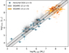 |
Fig. 1. Metal mass, MZ, ISM, vs. [C II] luminosity, L[CII]. The observed galaxy samples at z ≈ 0 (see text) with direct measurements of MZ, ISM and L[CII] are shown by the blue circles. The grey- and orange-shaded 2D hexagonal histograms represent simulated galaxies from SÍGAME-v2 (z ≈ 6) and v3 (z ≈ 0), and their mean and 1σ distributions are marked by the grey and orange squares respectively. The dashed line indicates the best-fit relation log(MZ, ISM/M⊙) = log(L[CII]/L⊙)−0.45 between all data sets and the grey-shaded region indicates the 0.4 dex rms scatter. |
2.2. Simulations of galaxies at z ≈ 0, 6
To support the observational data, we further include the recent simulations of galaxies through the Simulator of Galaxy Millimeter/submillimeter Emission (SÍGAME) framework (Olsen et al. 2017)1. This simulation provides detailed modelling of the far-infrared line emission from galaxies extracted from the particle-based cosmological hydrodynamics simulation Simba (Davé et al. 2019). We consider the results derived for galaxies at z ≈ 6 as part of the SÍGAME version 2 (v2) presented by Leung et al. (2020) and Vizgan et al. (2022a), and the more recent v3 results applicable to galaxies at z ≈ 0 (Olsen et al. 2021). To derive the metal masses for these simulated sets of galaxies, we used Eq. (1) above. Following Vizgan et al. (2022b), we represent MHI by the total “diffuse” H I component in the SÍGAME-v2 simulations, which is equal to the sum of its ionized and atomic hydrogen gas mass and distinct from the “dense” fraction of the mass of each fluid element, and extract directly the H I component from the SÍGAME-v3 model. For both simulations, we adopted the star formation rate weighted gas-phase metallicity, ZSFR, which best represent the metallicities of the H II regions inferred through the emission-line measurements.
2.3. The [C II]-to-MZ, ISM calibration
We compared the results from the simulated data sets to the observational dwarf galaxy sample at z ≈ 0 in Fig. 1. The SÍGAME-v2 simulations at z ≈ 6 best represent the observed data, as they cover a similarly broad range in the [C II] luminosities of L[CII] = 6.6 × 10³ − 8.1 × 10⁸ L⊙ and metal masses, MZ, ISM = 1.8 × 10⁴ − 1.0 × 10⁸ M⊙. The SÍGAME-v3 simulations mainly represent the high-L[CII], high-MZ, ISM parameter space, covering L[CII] = 5.3 × 10⁶ − 1.6 × 10⁹ L⊙, and MZ, ISM = 1.1 × 10⁶ − 6.7 × 10⁸ M⊙. We determined the correlation between L[CII] and MZ, ISM by first computing the Pearson r and p correlation coefficients using scipy’s stat module. For the simulations datasets, we considered the mean and standard deviations in bins of the data, as visualized in Fig. 1. This yields r = 0.93 and p = 7.6 × 10⁻¹¹, suggesting highly correlated data. Then, we used the linear regression module in Scikit to estimate the linear best-fit relation, in addition to the root mean square (rms) and the r2 scatter of the data. We found a slope consistent with unity (formally 0.91 ± 0.10), over more than five orders of magnitudes in L[CII] and MZ, ISM, with a unique constant ratio of
![Mathematical equation: $$ \begin{aligned} \log (M_{Z,\mathrm{ISM}}/M_\odot ) = \log (L_{\rm [CII]}/L_\odot ) - 0.45 \pm 0.40, \end{aligned} $$](/articles/aa/full_html/2023/10/aa46573-23/aa46573-23-eq4.gif) (2)
(2)
where the uncertainty represents the rms scatter, with an r2 value of 0.85.
To further test any potential offsets in the L[CII] − MZ, ISM relation, we show this ratio as a function of metallicity in Fig. 2. Here, we also include the relative abundance measurements from GRB absorption line spectroscopy derived by Heintz et al. (2021). This approach infers the “column” [C II] luminosity measured in the line of sight from the spontaneous decay of the excited C II* transition as ![Mathematical equation: $ L^{\mathrm{c}}_{\mathrm{[CII]}} = h\nu_{\mathrm{ul}}A_{\mathrm{ul}} N_{\mathrm{CII^*}} $](/articles/aa/full_html/2023/10/aa46573-23/aa46573-23-eq5.gif) . Here, NCII* is the column density of the 2P3/2 state of C+, and νul and Aul are the frequency and Einstein coefficient, respectively, of [C II]. We relate this column [C II] luminosity to the inferred line of sight metal mass,
. Here, NCII* is the column density of the 2P3/2 state of C+, and νul and Aul are the frequency and Einstein coefficient, respectively, of [C II]. We relate this column [C II] luminosity to the inferred line of sight metal mass, ![Mathematical equation: $ M^{\mathrm{c}}_{Z} = M_{\mathrm{HI}} \times 10^\mathrm{[M/H]_{tot}} \times Z_\odot $](/articles/aa/full_html/2023/10/aa46573-23/aa46573-23-eq6.gif) , with MHI being the H I column mass inferred from the column density as MHI = mHI × NHI and [M/H]tot the total absorption metallicity (equivalent to log Z/Z⊙). These GRB measurements provide accurate estimates of the L[CII] − MZ, ISM ratios only, in pencil-beam sightlines through their host galaxies (see also Heintz & Watson 2020).
, with MHI being the H I column mass inferred from the column density as MHI = mHI × NHI and [M/H]tot the total absorption metallicity (equivalent to log Z/Z⊙). These GRB measurements provide accurate estimates of the L[CII] − MZ, ISM ratios only, in pencil-beam sightlines through their host galaxies (see also Heintz & Watson 2020).
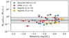 |
Fig. 2. MZ − L[CII] relation as a function of metallicity. Red hexagons show the inferred line-of-sight measurements from GRB sightlines (see text for details), the blue circles denote the observed galaxy samples at z ≈ 0 with direct measurements of MZ, ISM, and the average values of MZ/L[CII] in bins of 0.5 dex in metallicity predicted by the simulations at z ≈ 0 are shown as orange squares and at z ≈ 6 as the grey squares. The constant MZ − L[CII] ratio and the rms scatter of the data are shown by the dashed line and grey-shaded region, respectively. |
In Fig. 2, we compare the GRB measurements to the observational and simulated galaxy samples described above. We observe a remarkable agreement, with a mean GRB-inferred ratio of log(MZ, ISM/L[CII]) = − 0.44 ± 0.35 (error denoting 1σ). Moreover, the GRB sightlines probe galaxies in a large redshift range, z ∼ 2 − 6, and expand the metallicity regime for which we can determine the L[CII] − MZ, ISM relation, reproducing the constant ratio down to metallicities of Z/Z⊙ = 1%. We note, however, that the SÍGAME-v3 simulations potentially indicate an increasing MZ, ISM/L[CII] ratio around solar metallicities. This estimate is still within the overall scatter of the relation, yet it may indicate that [C II] emission is suppressed for a given metal mass in the highest metallicity galaxies. This could be due to more inefficient cooling through the [C II]−158 μm transition or potentially from lower ionization states. The relation between L[CII] and MZ, ISM derived here is purely an empirical result, based on direct observations and independent simulations, revealing an approximate constant ratio between the two. Crucially, this ratio appears to be constant across redshifts, making the conversion factor universally applicable.
3. Results
To apply the [C II]-to-MZ, ISM conversion factor, we compiled the recent high-z observational samples surveyed for [C II]: At z ∼ 2, we included the observations of main-sequence, star-forming galaxies from Zanella et al. (2018), whereas at z ∼ 4 − 6, we made use of the ALMA Large Program to Investigate C+ at Early Times (ALPINE) survey (Le Fèvre et al. 2020; Béthermin et al. 2020; Faisst et al. 2020) in addition to the sample of galaxies presented by Capak et al. (2015). At z ∼ 6 − 8, we consider the galaxies from the Reionization Era Bright Emission Line Survey (REBELS; Bouwens et al. 2022). In our analysis, we further include the individual measurements of A1689-zD1 (at z = 7.13; Watson et al. 2015; Bakx et al. 2021; Killi et al. 2023) and S04590 (at z = 8.496; Heintz et al. 2023) since both these high-z galaxies have robust estimates of their ISM gas masses and metallicities. The galaxy samples are all selected to have sufficient auxiliary data to enable derivations of the star formation rate (SFR) and stellar mass (M⋆) of each source, and to follow the star-forming galaxy main-sequence at their respective redshifts.
In Fig. 3, we show the inferred metal masses for the compiled sample of high-redshift (z ≳ 2) galaxies as a function of stellar mass. For all galaxies at z ≳ 2, except for A1689-zD1 and S04590, we infer the metal mass following the metallicity-independent conversion derived in Eq. (2), log(MZ, ISM/M⊙) = log(L[CII]/L⊙)−0.45 ± 0.40. For A1689-zD1, we infer MZ, ISM based on the derived approximate solar metallicity (Killi et al. 2023) and the H I gas mass MHI = 1.8 × 10¹⁰ M⊙, using the [C II]-to-H I conversion factor derived by Heintz et al. (2021), which yields MZ, ISM = 2.45 × 10⁸ M⊙ following Eq. (1). For S04590, we adopt the metal mass inferred by Heintz et al. (2023) of MZ, ISM = (3.2 ± 1.5)×105 M⊙, following a similar approach. These estimates are also in agreement with that inferred from the L[CII] − MZ, ISM calibrations for those particular sources. Overall, we find metal masses in the range MZ, ISM = 2 × 10⁷ − 109 M⊙, and observe that MZ, ISM generally increases with M⋆, which is expected given the increased metal yield for more abundant stellar populations. For comparison, we overplot the MZ, ISM(M⋆) function derived by Peeples et al. (2014) from the expected total Type II supernova metal production:
 (3)
(3)
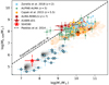 |
Fig. 3. Metal mass MZ, ISM as a function of stellar mass M⋆ for the compiled high-redshift galaxy sample survey for [C II]. Colors and symbols denote the respective surveys (see main text for details). The dashed line mark the expected total Type II supernova metal production as a function of M⋆ (Peeples et al. 2014). |
based on the star-formation histories by Leitner (2012). Here, y is the nucleosynthetic yields, which we assume to be y = 0.033 (Peeples et al. 2014). We note that these SFHs might be more extended than what is possible for early galaxies at z ≈ 4 − 7, simply due to the young age of the universe at these early times. Using more brief SFHs such that the enrichment is dominated by core-collapse supernovae (SNe), Sanders et al. (2023a) found that the total metal production is simply proportional to the product of the SNe metal yield, stellar mass, and (1 − R), where R is the return fraction. This method yields a consistent curve to that derived by Peeples et al. (2014), however, and therefore seems to well represent the expected metal yield also at high-z. Generally, high-redshift galaxies are observed to have MZ, ISM values that are lower than this predicted curve at any given stellar mass. We also note the potentially more significant offset at low stellar masses in Fig. 3.
We go on to consider the metal-to-stellar mass ratio, MZ, ISM/M⋆, for the compiled sample of galaxies as a function of redshift in Fig. 4. This ratio represents how effective galaxies are at retaining metals, given that M⋆ is approximately proportional to the total amounts of metals produced as prescribed in Eq. (3) (see also Peeples et al. 2014; Sanders et al. 2023a). For the galaxies at z ∼ 0, MZ, ISM are measured directly through the metallicities and gas masses of the galaxies in the sample. We determine  (median and 16th to 84th percentiles) at z ≈ 0. This increases to MZ, ISM/M⋆ ≈ 10−2, derived as the average for the sample of galaxies at z ∼ 2, and further to MZ, ISM/M⋆ ≈ 2 × 10⁻² at z ∼ 4 − 6 and MZ, ISM/M⋆ ≈ 5 × 10⁻² at z ≳ 6. As a reference point, we also include the stacked average of MZ, ISM/M⋆ ≈ 10−2 inferred by Sanders et al. (2023a) for galaxies at z ∼ 2 − 3. This result is based on rest-frame optical emission lines to infer metallicities and with gas masses inferred from CO, which may introduce a systematic difference compared to our method. Their results indicate that an increasing amount of metals reside in the gas-phase ISM in galaxies at higher redshifts, which also seem to hold for even the most massive systems (Sanders et al. 2023a). This likely reflects that feedback mechanisms or outflows are not yet efficient in expelling the metals out of the galaxy ISM at these epochs. On the contrary, most of the metals in local galaxies reside in stars (Peeples et al. 2014; Muratov et al. 2017).
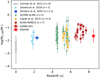 |
Fig. 4. Retained metal yield of the ISM, MZ, ISM/M⋆, as a function of redshift. Symbol notation follows that of Fig. 3, but now includes the benchmark z ≈ 0 galaxy sample, marked by dark- and light-gray boxes representing the 1σ and 2σ distributions of MZ, ISM/M⋆, in addition to the lensed galaxy S04590 from Heintz et al. (2023). |
4. The cosmic metal mass density in galaxies
To further quantify the chemical enrichment of galaxies through cosmic time, we now consider the cosmological metal mass density (ΩZ, ISM) and its evolution with redshift. Previously, it has only been possible to infer ΩZ, ISM at z ≳ 1 in quasar absorption-line systems (DLAs, e.g., Péroux & Howk 2020), since the metal abundances of high-z galaxies are generally difficult and time consuming to constrain through other approaches such as from nebular line emission and strong-line diagnostics (see e.g., Kewley et al. 2019; Maiolino & Mannucci 2019, for recent reviews). However, there is increasing evidence for DLAs to mainly probe the outskirts of their extended neutral, gaseous halos, in particular at z ≳ 3 (Neeleman et al. 2019; Stern et al. 2021; Yates et al. 2021; Heintz et al. 2022b). Therefore, these pencil-beam sightlines do not probe the central star-forming ISM of their galaxy counterparts, so it is imperative to establish alternative approaches to infer ΩZ, ISM in galaxies at the highest redshifts.
We determined ΩZ, ISM based on the derived [C II]−158 μm luminosity density, defined as ![Mathematical equation: $ \mathcal{L}_{\rm [CII]} = \int^{\infty}_{L_{\rm [CII]}} L_{\rm [CII]} \phi(L_{\rm [CII]}) {\rm d}L_{\rm [CII]} $](/articles/aa/full_html/2023/10/aa46573-23/aa46573-23-eq9.gif) , and the constant [C II]-to-MZ, ISM scaling derived here. This approach is similar to previous efforts determining the cosmic H2 gas mass density based on the CO luminosity density (e.g., Walter et al. 2014; Decarli et al. 2019; Riechers et al. 2019) and the H I gas mass density based on an empirical metallicity-dependent scaling to ℒ[CII] (Heintz et al. 2021, 2022b). Since [C II] traces the overall star-forming ISM, this approach provides a more direct measure of the mass of metals in the ISM of galaxies, compared to DLA sightlines. We here adopt the [C II]−158 μm luminosity densities derived by Oesch et al. (in prep.; see also Heintz et al. 2022b) at z ≈ 5 and z ≈ 7, based on the ALMA-ALPINE (Béthermin et al. 2020) and REBELS (Bouwens et al. 2022) surveys for [C II] emission from main-sequence galaxies at the respective redshifts. Integrating the [C II] luminosity function down to L[CII] = 107.5 L⊙, yields luminosity densities of
, and the constant [C II]-to-MZ, ISM scaling derived here. This approach is similar to previous efforts determining the cosmic H2 gas mass density based on the CO luminosity density (e.g., Walter et al. 2014; Decarli et al. 2019; Riechers et al. 2019) and the H I gas mass density based on an empirical metallicity-dependent scaling to ℒ[CII] (Heintz et al. 2021, 2022b). Since [C II] traces the overall star-forming ISM, this approach provides a more direct measure of the mass of metals in the ISM of galaxies, compared to DLA sightlines. We here adopt the [C II]−158 μm luminosity densities derived by Oesch et al. (in prep.; see also Heintz et al. 2022b) at z ≈ 5 and z ≈ 7, based on the ALMA-ALPINE (Béthermin et al. 2020) and REBELS (Bouwens et al. 2022) surveys for [C II] emission from main-sequence galaxies at the respective redshifts. Integrating the [C II] luminosity function down to L[CII] = 107.5 L⊙, yields luminosity densities of ![Mathematical equation: $ \log (\mathcal{L}_{\mathrm{[CII]}}/L_\odot\,\mathrm{Mpc}^{-3}) = 5.37^{+0.19}_{-0.16} $](/articles/aa/full_html/2023/10/aa46573-23/aa46573-23-eq10.gif) (at z ≈ 5) and
(at z ≈ 5) and ![Mathematical equation: $ \log (\mathcal{L}_{\mathrm{[CII]}}/L_\odot\,\mathrm{Mpc}^{-3}) = 4.85^{+0.25}_{-0.20} $](/articles/aa/full_html/2023/10/aa46573-23/aa46573-23-eq11.gif) (at z ≈ 7). Applying the [C II]-to-MZ, ISM calibration, we derive metal mass densities of
(at z ≈ 7). Applying the [C II]-to-MZ, ISM calibration, we derive metal mass densities of  and
and  , at z ≈ 5 and z ≈ 7, respectively. In Fig. 5, we also show the inferred
  at z ≈ 0 based on the [C II] luminosity function derived by Hemmati et al. (2017) at a similar redshift.
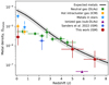 |
Fig. 5. Cosmological density of metals as a function of redshift. Red hexagons show the measurements from this work based on the [C II] luminosity densities at z ≈ 5 and ≈7, converted to ΩZ, ISM. The other symbols represent the metal densities inferred by various approaches, color-coded as a function of the distinct gas phases they are probing from the compilation of Péroux & Howk (2020), including results from Sanders et al. (2023a) and with the purple triangle denoting the lower bound derived from O I absorption at z ≈ 6 in sub-DLAs by Becker et al. (2011). The solid black line shows the expected yield of metals from star formation, assuming ΩZ(z) = yΩ⋆(z), with y = 0.033 being the integrated yield of the stellar population and Ω⋆(z) is the stellar mass density quantified by Walter et al. (2020). These measurements suggest that metals mostly reside in the ISM of galaxies at z ≳ 3. |
We highlight our measurements in Fig. 5 as the red hexagons. For comparison, we show the total expected metal yield from stars, defined as ΩZ, ⋆(z) = yρ⋆(z)/ρc, where y is the integrated yield of the stellar population, ρ⋆(z) the stellar mass density, and ρc is the critical density of the universe. Here, we adopt y = 0.033 from Peeples et al. (2014; see also Péroux & Howk 2020), the evolutionary function of ρ⋆(z) parametrized by Walter et al. (2020)2, and ρc= 1.26 × 10¹¹ M⊙ Mpc−3 from the concordance ΛCDM cosmological framework (Planck Collaboration VI 2020). We find that our measurements are in remarkable agreement with the metal yield predicted by ΩZ, ⋆(z) at z ≳ 4. This suggests that the majority of metals are confined to the galaxy central ISM (as also discussed in Sect. 3) and have not yet been expelled to the outer regions through outflows and feedback effects. This suggests that the origin of the extended [C II] halos are likely not caused by outflows (as previously proposed, e.g., Maiolino et al. 2012; Cicone et al. 2015; Ginolfi et al. 2020b; Herrera-Camus et al. 2021; Akins et al. 2022), but supports the scenario where the [C II] emission instead traces the extended neutral gas reservoirs (Novak et al. 2019, 2020; Harikane et al. 2020; Heintz et al. 2021, 2022b; Meyer et al. 2022). In this case, there would be some small, but not negligible, in situ star formation in the extended neutral gas disks. Further, these results provide additional evidence for the robustness of the [C II]-to-MZ, ISM scaling relation derived in this work. At z ∼ 0, we also find that only ≈10% of the expected metal yield resides in the ISM of galaxies, consistent with DLA studies (Péroux & Howk 2020).
In Fig. 5 we additionally compare our measurements to estimates of ΩZ, ISM inferred through various approaches and for different baryonic phases: metals associated with the neutral gas probed via DLAs, metals located in the hot intracluster medium (ICM) and partially ionized gas, as well as the mass of metals attained in stars (see Péroux & Howk 2020, and references therein). We find that our ΩZ, ISM estimates inferred from [C II] are in good agreement with the DLA measurements at z ≳ 3, showing a consistent decrease in the metal mass density with increasing redshift following that expected from the stellar yield, ΩZ, ⋆(z). Direct DLA measurements are, however, only possible out to z ≈ 5 due to the increasing suppression of the emission located in the Lyman-α forest caused by the Gunn-Peterson effect at these redshifts. Becker et al. (2011) attempted to partly alleviate this by measuring the density of O I absorption at z ≈ 6 in sub-DLAs (probing partly ionized gas down to NHI = 1019 cm−2). This point is shown as a lower bound on ΩZ, ISM in Fig. 5 since ΩZ, ISM ≳ ΩOI. The method presented here thus provides a complementary census of the high-redshift metal mass density, at previous inaccessible epochs. At z ≲ 1, most of the metals are observed to be captured in stars (Péroux & Howk 2020).
Comparing our measurements of ΩZ, ISM at z ≈ 5 and ≈7 to Ωdust at equivalent redshifts, we can further make the first prediction for the volume-averaged dust-to-metals (DTM) ratio at these epochs. Based on the recent simulations by GADGET3-OSAKA (Aoyama et al. 2018) and GIZMO-SIMBA (Li et al. 2019), in addition to the results quasar DLA measurements (Péroux & Howk 2020), we find that Ωdust/ΩZ ≈ 10% at z ≳ 5, about a factor of 5 lower than the Milky Way average (DTMGal ≈ 50%, by mass).
5. Conclusions
In an attempt to establish an independent, complementary way of inferring the total ISM metal mass of galaxies, MZ, ISM, we have derived an empirical scaling between the [C II]−158 μm line luminosity and MZ, ISM. This scaling is determined from an observational benchmark sample of galaxies at z ≈ 0, where MZ, ISM could be estimated directly through the metallicity and H I gas mass of the galaxies, in addition to recent hydrodynamical simulations of galaxies at z ≈ 0 and z ≈ 6. The [C II]-to-MZ, ISM ratio appears universal across redshifts and constant through more than two orders of magnitude in metallicity, with a ratio of log(MZ, ISM/M⊙) = log(L[CII]/L⊙)−0.45 (and 0.4 dex scatter).
We applied this calibration to recent high-z (z ≳ 2) surveys for the [C II] line emission from main-sequence galaxies reaching well into the epoch of reionization at z ≈ 8. We derived ISM metal masses in the range of MZ, ISM = 2 × 10⁷ − 109 M⊙ and found that the metal-to-stellar mass of these galaxies increases with increasing redshift. This ratio effectively describes how galaxies are increasingly efficient at retaining the produced stellar metal yield at higher redshifts, suggesting that most of the produced metals at early cosmic epochs are confined to the ISM of galaxies. This has potential important implications for outflow processes at these redshifts, which may be less substantial than previously reported.
Using the same [C II]-to-MZ, ISM calibration and recent estimates of the [C II] luminosity density at z ≈ 5 and ≈7, we further placed indirect constraints on the cosmological metal mass density ΩZ, ISM at these redshifts. We found that these estimates were consistent with predictions of the total metal yield from stars, based on a recent empirical parametrization of the stellar mass density. Our measurements were therefore able to account for the total expected metal budget at these redshifts, indicating that, on average, most of the metals produced from stellar explosions are still confined to the local ISM of these galaxies. At lower redshifts, z ≈ 0 − 2, most of the metals are found in other forms, predominantly stars (Péroux & Howk 2020; Sanders et al. 2023a). Further comparing our measurements of ΩZ, ISM to Ωdust measured from quasar DLAs, and with recent simulations, we found that Ωdust/ΩZ, ISM ≈10% at z ≳ 5, a factor of ≈5 lower than the Galactic average.
In the near-future, the James Webb Space Telescope (JWST) will be able to routinely enable measurements of the metallicity of galaxies well into the epoch of reionization at z ≳ 6, as previously demonstrated by the early release science data (see e.g., Trump et al. 2023; Schaerer et al. 2022; Rhoads et al. 2023; Curti et al. 2023; Arellano-Córdova et al. 2022; Brinchmann 2023; Heintz et al. 2023) and the recent results from the Cosmic Evolution Early Release Science (CEERS) survey (Finkelstein et al. 2023, see Heintz et al. 2022a; Nakajima et al. 2023; Fujimoto et al. 2023; Sanders et al. 2023b). In combination with the gas masses inferred from ALMA observations through proxies such as [C II] (e.g., Heintz et al. 2022b) and the far-infrared continuum revealing the dust content (Inami et al. 2022; Dayal et al. 2022), it will soon be possible to directly measure the ISM metal mass and the DTM ratio of galaxies during the earliest cosmic epochs, as recently demonstrated in the case-study by Heintz et al. (2023). This was enabled by combining ALMA and JWST observations of a lensed galaxy at z ≈ 8.5.
Converted to a Chabrier IMF.
Acknowledgments
We would like to thank the referee for a carefully reviewing this paper and for their suggestions that greatly improved the presentation of the results in this work. K.E.H. acknowledges support from the Carlsberg Foundation Reintegration Fellowship Grant CF21-0103. The Cosmic Dawn Center (DAWN) is funded by the Danish National Research Foundation under grant no. 140. Source codes for the figures and tables presented in this manuscript are available from the corresponding author upon reasonable request.
References
- Akins, H. B., Fujimoto, S., Finlator, K., et al. 2022, ApJ, 934, 64 [NASA ADS] [CrossRef] [Google Scholar]
- Aoyama, S., Hou, K.-C., Hirashita, H., Nagamine, K., & Shimizu, I. 2018, MNRAS, 478, 4905 [NASA ADS] [CrossRef] [Google Scholar]
- Arellano-Córdova, K. Z., Berg, D. A., Chisholm, J., et al. 2022, ApJ, 940, L23 [CrossRef] [Google Scholar]
- Asplund, M., Grevesse, N., Sauval, A. J., & Scott, P. 2009, ARA&A, 47, 481 [NASA ADS] [CrossRef] [Google Scholar]
- Bakx, T. J. L. C., Sommovigo, L., Carniani, S., et al. 2021, MNRAS, 508, L58 [NASA ADS] [CrossRef] [Google Scholar]
- Becker, G. D., Sargent, W. L. W., Rauch, M., & Calverley, A. P. 2011, ApJ, 735, 93 [NASA ADS] [CrossRef] [Google Scholar]
- Béthermin, M., Fudamoto, Y., Ginolfi, M., et al. 2020, A&A, 643, A2 [Google Scholar]
- Bouché, N., Lehnert, M. D., Aguirre, A., Péroux, C., & Bergeron, J. 2007, MNRAS, 378, 525 [CrossRef] [Google Scholar]
- Bouwens, R. J., Smit, R., Schouws, S., et al. 2022, ApJ, 931, 160 [NASA ADS] [CrossRef] [Google Scholar]
- Brinchmann, J. 2023, MNRAS, 525, 2087 [NASA ADS] [CrossRef] [Google Scholar]
- Capak, P. L., Carilli, C., Jones, G., et al. 2015, Nature, 522, 455 [NASA ADS] [CrossRef] [Google Scholar]
- Chabrier, G. 2003, PASP, 115, 763 [Google Scholar]
- Cicone, C., Maiolino, R., Gallerani, S., et al. 2015, A&A, 574, A14 [NASA ADS] [CrossRef] [EDP Sciences] [Google Scholar]
- Cormier, D., Madden, S. C., Lebouteiller, V., et al. 2015, A&A, 578, A53 [CrossRef] [EDP Sciences] [Google Scholar]
- Curti, M., D’Eugenio, F., Carniani, S., et al. 2023, MNRAS, 518, 425 [Google Scholar]
- Davé, R., Anglés-Alcázar, D., Narayanan, D., et al. 2019, MNRAS, 486, 2827 [Google Scholar]
- Dayal, P., Ferrara, A., Sommovigo, L., et al. 2022, MNRAS, 512, 989 [NASA ADS] [CrossRef] [Google Scholar]
- Decarli, R., Walter, F., Gónzalez-López, J., et al. 2019, ApJ, 882, 138 [Google Scholar]
- Dessauges-Zavadsky, M., Ginolfi, M., Pozzi, F., et al. 2020, A&A, 643, A5 [NASA ADS] [CrossRef] [EDP Sciences] [Google Scholar]
- Draine, B. T., Dale, D. A., Bendo, G., et al. 2007, ApJ, 663, 866 [NASA ADS] [CrossRef] [Google Scholar]
- Dwek, E. 1998, ApJ, 501, 643 [NASA ADS] [CrossRef] [Google Scholar]
- Eales, S., Gomez, H., Dunne, L., Dye, S., & Smith, M. W. L. 2023, MNRAS, submitted [arXiv:2303.07376] [Google Scholar]
- Faisst, A. L., Schaerer, D., Lemaux, B. C., et al. 2020, ApJS, 247, 61 [NASA ADS] [CrossRef] [Google Scholar]
- Fall, S. M., & Pei, Y. C. 1993, ApJ, 402, 479 [NASA ADS] [CrossRef] [Google Scholar]
- Ferrara, A., Scannapieco, E., & Bergeron, J. 2005, ApJ, 634, L37 [NASA ADS] [CrossRef] [Google Scholar]
- Finkelstein, S. L., Bagley, M. B., Ferguson, H. C., et al. 2023, ApJ, 946, L13 [NASA ADS] [CrossRef] [Google Scholar]
- Fujimoto, S., Haro, P. A., Dickinson, M., et al. 2023, ApJ, 949, L25 [NASA ADS] [CrossRef] [Google Scholar]
- Gall, C., Hjorth, J., Watson, D., et al. 2014, Nature, 511, 326 [CrossRef] [Google Scholar]
- Ginolfi, M., Hunt, L. K., Tortora, C., Schneider, R., & Cresci, G. 2020a, A&A, 638, A4 [NASA ADS] [CrossRef] [EDP Sciences] [Google Scholar]
- Ginolfi, M., Jones, G. C., Béthermin, M., et al. 2020b, A&A, 633, A90 [NASA ADS] [CrossRef] [EDP Sciences] [Google Scholar]
- Harikane, Y., Ouchi, M., Inoue, A. K., et al. 2020, ApJ, 896, 93 [Google Scholar]
- Heintz, K. E., & Watson, D. 2020, ApJ, 889, L7 [Google Scholar]
- Heintz, K. E., Fynbo, J. P. U., Ledoux, C., et al. 2018, A&A, 615, A43 [NASA ADS] [CrossRef] [EDP Sciences] [Google Scholar]
- Heintz, K. E., Watson, D., Oesch, P. A., Narayanan, D., & Madden, S. C. 2021, ApJ, 922, 147 [NASA ADS] [CrossRef] [Google Scholar]
- Heintz, K. E., Brammer, G. B., Giménez-Arteaga, C., et al. 2022a, ArXiv e-prints [arXiv:2212.02890] [Google Scholar]
- Heintz, K. E., Oesch, P. A., Aravena, M., et al. 2022b, ApJ, 934, L27 [NASA ADS] [CrossRef] [Google Scholar]
- Heintz, K. E., Giménez-Arteaga, C., Fujimoto, S., et al. 2023, ApJ, 944, L30 [NASA ADS] [CrossRef] [Google Scholar]
- Hemmati, S., Yan, L., Diaz-Santos, T., et al. 2017, ApJ, 834, 36 [Google Scholar]
- Herrera-Camus, R., Förster Schreiber, N., Genzel, R., et al. 2021, A&A, 649, A31 [NASA ADS] [CrossRef] [EDP Sciences] [Google Scholar]
- Hollenbach, D. J., & Tielens, A. G. G. M. 1999, Rev. Mod. Phys., 71, 173 [Google Scholar]
- Hunt, L. K., Tortora, C., Ginolfi, M., & Schneider, R. 2020, A&A, 643, A180 [NASA ADS] [CrossRef] [EDP Sciences] [Google Scholar]
- Inami, H., Algera, H. S. B., Schouws, S., et al. 2022, MNRAS, 515, 3126 [NASA ADS] [CrossRef] [Google Scholar]
- Kewley, L. J., Nicholls, D. C., & Sutherland, R. S. 2019, ARA&A, 57, 511 [Google Scholar]
- Killi, M., Watson, D., Fujimoto, S., et al. 2023, MNRAS, 521, 2526 [NASA ADS] [CrossRef] [Google Scholar]
- Krogager, J.-K., Fynbo, J. P. U., Møller, P., et al. 2019, MNRAS, 486, 4377 [NASA ADS] [CrossRef] [Google Scholar]
- Lagache, G., Cousin, M., & Chatzikos, M. 2018, A&A, 609, A130 [NASA ADS] [CrossRef] [EDP Sciences] [Google Scholar]
- Le Fèvre, O., Béthermin, M., Faisst, A., et al. 2020, A&A, 643, A1 [Google Scholar]
- Leitner, S. N. 2012, ApJ, 745, 149 [NASA ADS] [CrossRef] [Google Scholar]
- Leroy, A. K., Walter, F., Bigiel, F., et al. 2009, AJ, 137, 4670 [Google Scholar]
- Leśniewska, A., & Michałowski, M. J. 2019, A&A, 624, L13 [Google Scholar]
- Leung, T. K. D., Olsen, K. P., Somerville, R. S., et al. 2020, ApJ, 905, 102 [NASA ADS] [CrossRef] [Google Scholar]
- Li, Q., Narayanan, D., & Davé, R. 2019, MNRAS, 490, 1425 [CrossRef] [Google Scholar]
- Liang, L., Feldmann, R., Murray, N., et al. 2023, ArXiv e-prints [arXiv:2301.04149] [Google Scholar]
- Madden, S. C., Poglitsch, A., Geis, N., Stacey, G. J., & Townes, C. H. 1997, ApJ, 483, 200 [NASA ADS] [CrossRef] [Google Scholar]
- Madden, S. C., Rémy-Ruyer, A., Galametz, M., et al. 2013, PASP, 125, 600 [NASA ADS] [CrossRef] [Google Scholar]
- Madden, S. C., Cormier, D., Hony, S., et al. 2020, A&A, 643, A141 [NASA ADS] [CrossRef] [EDP Sciences] [Google Scholar]
- Maiolino, R., & Mannucci, F. 2019, A&ARv, 27, 3 [Google Scholar]
- Maiolino, R., Nagao, T., Grazian, A., et al. 2008, A&A, 488, 463 [NASA ADS] [CrossRef] [EDP Sciences] [Google Scholar]
- Maiolino, R., Gallerani, S., Neri, R., et al. 2012, MNRAS, 425, L66 [Google Scholar]
- Meyer, R. A., Walter, F., Cicone, C., et al. 2022, ApJ, 927, 152 [NASA ADS] [CrossRef] [Google Scholar]
- Morselli, L., Renzini, A., Enia, A., & Rodighiero, G. 2021, MNRAS, 502, L85 [NASA ADS] [CrossRef] [Google Scholar]
- Muratov, A. L., Kereš, D., Faucher-Giguère, C.-A., et al. 2017, MNRAS, 468, 4170 [NASA ADS] [CrossRef] [Google Scholar]
- Nakajima, K., Ouchi, M., Isobe, Y., et al. 2023, ApJS, submitted [arXiv:2301.12825] [Google Scholar]
- Neeleman, M., Kanekar, N., Prochaska, J. X., Rafelski, M. A., & Carilli, C. L. 2019, ApJ, 870, L19 [NASA ADS] [CrossRef] [Google Scholar]
- Novak, M., Bañados, E., Decarli, R., et al. 2019, ApJ, 881, 63 [NASA ADS] [CrossRef] [Google Scholar]
- Novak, M., Venemans, B. P., Walter, F., et al. 2020, ApJ, 904, 131 [NASA ADS] [CrossRef] [Google Scholar]
- Olsen, K., Greve, T. R., Narayanan, D., et al. 2017, ApJ, 846, 105 [Google Scholar]
- Olsen, K. P., Burkhart, B., Mac Low, M.-M., et al. 2021, ApJ, 922, 88 [NASA ADS] [CrossRef] [Google Scholar]
- Pallottini, A., Ferrara, A., Decataldo, D., et al. 2019, MNRAS, 487, 1689 [Google Scholar]
- Peeples, M. S., Werk, J. K., Tumlinson, J., et al. 2014, ApJ, 786, 54 [NASA ADS] [CrossRef] [Google Scholar]
- Péroux, C., & Howk, J. C. 2020, ARA&A, 58, 363 [CrossRef] [Google Scholar]
- Pettini, M., Ellison, S. L., Steidel, C. C., & Bowen, D. V. 1999, ApJ, 510, 576 [NASA ADS] [CrossRef] [Google Scholar]
- Pilyugin, L. S., & Thuan, T. X. 2005, ApJ, 631, 231 [CrossRef] [Google Scholar]
- Pineda, J. L., Langer, W. D., & Goldsmith, P. F. 2014, A&A, 570, A121 [NASA ADS] [CrossRef] [EDP Sciences] [Google Scholar]
- Planck Collaboration VI. 2020, A&A, 641, A6 [NASA ADS] [CrossRef] [EDP Sciences] [Google Scholar]
- Prochaska, J. X., Gawiser, E., Wolfe, A. M., Castro, S., & Djorgovski, S. G. 2003, ApJ, 595, L9 [NASA ADS] [CrossRef] [Google Scholar]
- Ramos Padilla, A. F., Wang, L., van der Tak, F. F. S., & Trager, S. 2023, A&A, in press https://doi.org/10.1051/0004-6361/202243358 [Google Scholar]
- Rémy-Ruyer, A., Madden, S. C., Galliano, F., et al. 2014, A&A, 563, A31 [Google Scholar]
- Rhoads, J. E., Wold, I. G. B., Harish, S., et al. 2023, ApJ, 942, L14 [NASA ADS] [CrossRef] [Google Scholar]
- Riechers, D. A., Pavesi, R., Sharon, C. E., et al. 2019, ApJ, 872, 7 [Google Scholar]
- Sanders, R. L., Shapley, A. E., Jones, T., et al. 2021, ApJ, 914, 19 [CrossRef] [Google Scholar]
- Sanders, R. L., Shapley, A. E., Jones, T., et al. 2023a, ApJ, 942, 24 [NASA ADS] [CrossRef] [Google Scholar]
- Sanders, R. L., Shapley, A. E., Topping, M. W., Reddy, N. A., & Brammer, G. B. 2023b, ApJ, submitted [arXiv:2303.08149] [Google Scholar]
- Schaerer, D., Marques-Chaves, R., Barrufet, L., et al. 2022, A&A, 665, L4 [NASA ADS] [CrossRef] [EDP Sciences] [Google Scholar]
- Scoville, N., Aussel, H., Sheth, K., et al. 2014, ApJ, 783, 84 [CrossRef] [Google Scholar]
- Scoville, N., Lee, N., Vanden Bout, P., et al. 2017, ApJ, 837, 150 [Google Scholar]
- Sommovigo, L., Ferrara, A., Carniani, S., et al. 2021, MNRAS, 503, 4878 [NASA ADS] [CrossRef] [Google Scholar]
- Sommovigo, L., Ferrara, A., Pallottini, A., et al. 2022, MNRAS, 513, 3122 [NASA ADS] [CrossRef] [Google Scholar]
- Stacey, G. J., Hailey-Dunsheath, S., Ferkinhoff, C., et al. 2010, ApJ, 724, 957 [NASA ADS] [CrossRef] [Google Scholar]
- Stern, J., Sternberg, A., Faucher-Giguère, C.-A., et al. 2021, MNRAS, 507, 2869 [NASA ADS] [CrossRef] [Google Scholar]
- Trump, J. R., Arrabal Haro, P., Simons, R. C., et al. 2023, ApJ, 945, 35 [NASA ADS] [CrossRef] [Google Scholar]
- Vallini, L., Ferrara, A., Pallottini, A., & Gallerani, S. 2017, MNRAS, 467, 1300 [NASA ADS] [Google Scholar]
- Vizgan, D., Greve, T. R., Olsen, K. P., et al. 2022a, ApJ, 929, 92 [NASA ADS] [CrossRef] [Google Scholar]
- Vizgan, D., Heintz, K. E., Greve, T. R., et al. 2022b, ApJ, 939, L1 [NASA ADS] [CrossRef] [Google Scholar]
- Walter, F., Decarli, R., Sargent, M., et al. 2014, ApJ, 782, 79 [NASA ADS] [CrossRef] [Google Scholar]
- Walter, F., Carilli, C., Neeleman, M., et al. 2020, ApJ, 902, 111 [Google Scholar]
- Watson, D., Christensen, L., Knudsen, K. K., et al. 2015, Nature, 519, 327 [Google Scholar]
- Wolfire, M. G., McKee, C. F., Hollenbach, D., & Tielens, A. G. G. M. 2003, ApJ, 587, 278 [Google Scholar]
- Yates, R. M., Péroux, C., & Nelson, D. 2021, MNRAS, 508, 3535 [NASA ADS] [CrossRef] [Google Scholar]
- Zanella, A., Daddi, E., Magdis, G., et al. 2018, MNRAS, 481, 1976 [Google Scholar]
All Figures
|
Fig. 1. Metal mass, MZ, ISM, vs. [C II] luminosity, L[CII]. The observed galaxy samples at z ≈ 0 (see text) with direct measurements of MZ, ISM and L[CII] are shown by the blue circles. The grey- and orange-shaded 2D hexagonal histograms represent simulated galaxies from SÍGAME-v2 (z ≈ 6) and v3 (z ≈ 0), and their mean and 1σ distributions are marked by the grey and orange squares respectively. The dashed line indicates the best-fit relation log(MZ, ISM/M⊙) = log(L[CII]/L⊙)−0.45 between all data sets and the grey-shaded region indicates the 0.4 dex rms scatter. |
| In the text | |
|
Fig. 2. MZ − L[CII] relation as a function of metallicity. Red hexagons show the inferred line-of-sight measurements from GRB sightlines (see text for details), the blue circles denote the observed galaxy samples at z ≈ 0 with direct measurements of MZ, ISM, and the average values of MZ/L[CII] in bins of 0.5 dex in metallicity predicted by the simulations at z ≈ 0 are shown as orange squares and at z ≈ 6 as the grey squares. The constant MZ − L[CII] ratio and the rms scatter of the data are shown by the dashed line and grey-shaded region, respectively. |
| In the text | |
|
Fig. 3. Metal mass MZ, ISM as a function of stellar mass M⋆ for the compiled high-redshift galaxy sample survey for [C II]. Colors and symbols denote the respective surveys (see main text for details). The dashed line mark the expected total Type II supernova metal production as a function of M⋆ (Peeples et al. 2014). |
| In the text | |
|
Fig. 4. Retained metal yield of the ISM, MZ, ISM/M⋆, as a function of redshift. Symbol notation follows that of Fig. 3, but now includes the benchmark z ≈ 0 galaxy sample, marked by dark- and light-gray boxes representing the 1σ and 2σ distributions of MZ, ISM/M⋆, in addition to the lensed galaxy S04590 from Heintz et al. (2023). |
| In the text | |
|
Fig. 5. Cosmological density of metals as a function of redshift. Red hexagons show the measurements from this work based on the [C II] luminosity densities at z ≈ 5 and ≈7, converted to ΩZ, ISM. The other symbols represent the metal densities inferred by various approaches, color-coded as a function of the distinct gas phases they are probing from the compilation of Péroux & Howk (2020), including results from Sanders et al. (2023a) and with the purple triangle denoting the lower bound derived from O I absorption at z ≈ 6 in sub-DLAs by Becker et al. (2011). The solid black line shows the expected yield of metals from star formation, assuming ΩZ(z) = yΩ⋆(z), with y = 0.033 being the integrated yield of the stellar population and Ω⋆(z) is the stellar mass density quantified by Walter et al. (2020). These measurements suggest that metals mostly reside in the ISM of galaxies at z ≳ 3. |
| In the text | |
Current usage metrics show cumulative count of Article Views (full-text article views including HTML views, PDF and ePub downloads, according to the available data) and Abstracts Views on Vision4Press platform.
Data correspond to usage on the plateform after 2015. The current usage metrics is available 48-96 hours after online publication and is updated daily on week days.
Initial download of the metrics may take a while.