| Issue |
A&A
Volume 684, April 2024
|
|
|---|---|---|
| Article Number | A203 | |
| Number of page(s) | 12 | |
| Section | Numerical methods and codes | |
| DOI | https://doi.org/10.1051/0004-6361/202449193 | |
| Published online | 26 April 2024 | |
Emulating the interstellar medium chemistry with neural operators
Scuola Normale Superiore,
Piazza dei Cavalieri 7,
56126
Pisa,
Italy
e-mail: This email address is being protected from spambots. You need JavaScript enabled to view it.
Received:
9
January
2024
Accepted:
15
February
2024
Abstract
Context. The study of galaxy formation and evolution critically depends on our understanding of the complex photo-chemical processes that govern the evolution and thermodynamics of the interstellar medium (ISM). In a computational sense, resolving the chemistry is among the weightiest tasks in cosmological and astrophysical simulations.
Aims. Astrophysical simulations can include photo-chemical models that allow for a wide range of densities (n), abundances of different species (ni/n) and temperature (T), and plausible evolution scenarios of the ISM under the action of a radiation field (F) with different spectral shapes and intensities. The evolution of such a non-equilibrium photo-chemical network relies on implicit, precise, computationally costly, ordinary differential equations (ODE) solvers. Here, we aim to substitute such procedural solvers with fast, pre-trained emulators based on neural operators.
Methods. We emulated a non-equilibrium chemical network up to H2 formation (9 species, 52 reactions) by adopting the DeepONet formalism, namely: by splitting the ODE solver operator that maps the initial conditions and time evolution into a tensor product of two neural networks (named branch and trunk). We used KROME to generate a training set, spanning −2 < log(n/cm−3) ≤ 3.5, log(20) ≤ log(T/K) ≤ 5.5, −6 ≤ log(ni/n) < 0, and adopting an incident radiation field, F, sampled in 10 energy bins with a continuity prior. We separately trained the solver for T and each ni for ≃4.34 GPUhrs.
Results. Compared with the reference solutions obtained by KROME for single-zone models, the typical precision obtained is of the order of 10−2, that is, it is 10 times better when using a training that is 40 times less costly, with respect to previous emulators that only considered a fixed F. DeepONet also performs well for T and ni outside the range of the training sample. Furthermore, the emulator aptly reproduces the ion and temperature profiles of photo dissociation regions as well; namely, by giving errors that are comparable to the typical difference between various photo-ionization codes. The present model achieves a speed-up of a factor of 128× with respect to stiff ODE solvers.
Conclusions. Our neural emulator represents a significant leap forward in the modelling of ISM chemistry, offering a good balance of precision, versatility, and computational efficiency. Nevertheless, further work is required to address the challenges represented by the extrapolation beyond the training time domain and the removal of potential outliers.
Key words: astrochemistry / methods: numerical / ISM: clouds / evolution / ISM: molecules
© The Authors 2024
 Open Access article, published by EDP Sciences, under the terms of the Creative Commons Attribution License (https://creativecommons.org/licenses/by/4.0), which permits unrestricted use, distribution, and reproduction in any medium, provided the original work is properly cited.
This article is published in open access under the Subscribe to Open model. This email address is being protected from spambots. You need JavaScript enabled to view it. to support open access publication.
1 Introduction
Non-equilibrium photo-chemistry plays a crucial role in many astrophysical and cosmological environments. Chemistry regulates the physical processes starting from cosmological scales (Galli & Palla 1998; Glover & Abel 2008) and it is key to understanding the evolution of the intergalactic medium (IGM) during the Epoch of Reionization (EoR, Theuns et al. 1998; Maio et al. 2007; Rosdahl et al. 2018). It has a significant impact in the formation and evolution of galaxies (Pallottini et al. 2017; Lupi 2019), in particular, by regulating the birth of giant molecular clouds (GMC, Decataldo et al. 2019; Kim et al. 2018) in the interstellar medium (ISM), and it continues to play a vital role down to the formation of planets (Caselli & Ceccarelli 2012).
From a theoretical point of view, these widely different environments are studied by developing astrophysical and cosmological simulations. To follow the thermo-chemical evolution in such simulations, it is necessary to solve the system of ordinary differential equations (ODEs) associated with it. Depending on the specific problem, various software has been developed and used to include chemical non-equilibrium chemistry in numerical codes. On the one hand, some codes allow for extensive photo-chemical network and offer a high level of precision; thus, they are expensive, such as CLOUDY (Ferland et al. 2017), UCLCHEM (Holdship et al. 2017), and MAIHEM (Gray et al. 2019). This kind of approach (see Olsen et al. 2018, for a review) is typically more suitable for post-processing astrophysical simulations to obtain emission lines (e.g. Vallini et al. 2018), since on-the-fly direct coupling is commonly limited to 1D simulations, such as photo-chemical evolutionary patterns that are solved during shock processes (e.g. Danehkar et al. 2022). On the other hand, some software are designed to be coupled to code for full 3D hydrodynamic evolution, such as ASTROCHEM (Kumar & Fisher 2013) and KROME (Grassi et al. 2014). These interfaces take, as their input, a user defined chemical network to prepare the code needed to solve the associated ODE system. We also have NIRVANA (Ziegler 2016) and GRACKLE (Smith et al. 2017), which are libraries that provide subroutines to solve selected types of chemical networks that are of astrophysical interest.
Coupling the chemistry evolution with an astrophysical code is challenging, mainly since the chemical ODE system is often stiff and the typical timescales are much shorter than the dynamical and hydrodynamic time, for instance: ∆tchem ≪ 10−4∆thydro. This implies that robust, multi-step, embedded, high-order (and, thus, costly) numerical solvers should be selected (e.g. Hindmarsh 2019). Furthermore, in terms of number of reactions, the complexity of the system grows more than linearly with respect to the number of species included in the chemical network. Finally, we consider that in numerical simulations, the domain is usually split on the basis of the time-steps hierarchy to balance between different processors the cost of gravity evaluation and hydrodynamical computation (Springel et al. 2021), while it is difficult to estimate the time-to-completion of the chemistry solver given the initial conditions (Branca & Pallottini 2023), implying the inclusion of such a task can spoil the load balancing. To overcome these limitations, various methods based on deep learning have been developed in recent years. In Holdship et al. (2021), the CHEMULATOR algorithm is introduced in order to emulate UCLCHEM (Holdship et al. 2017); it utilizes a combination of autoencoders and principal component analysis (PCA) to reduce the dimensionality of the chemical network (from 33 down to 8 dimensions); subsequently, a standard feed-forward neural network (FNN) is employed to predict the evolution of latent space variables. For the same kind of complex chemical system, in Heyl et al. (2023) the interpretability of the network is showcased by applying the SHAP coefficient calculation (Lundberg et al. 2018) to UCLCHEM precomputed tables interpolated via the eXtreme Gradient Boosting XGboost (Chen & Guestrin 2016) regressor. Further, machine learning techniques such as random forest (RF) can be used in conjunction with libraries of precise photoionization models in order to quickly predict the line emission from numerical simulations (Katz et al. 2019) or infer the basic ISM properties from observed line ratios (Ucci et al. 2018). Heading in the direction of a coupling with numerical simulation, Robinson et al. (2024) presented the feasibility of constructing an emulator utilizing XGboost for computing gas heating and cooling tables obtained from Gnedin & Hollon (2012). This approach relies on accurate CLOUDY (Ferland et al. 2017) models for the training, however, it does not account for the evolution of chemical species (see also Galligan et al. 2019, for an emulator for cooling). Meanwhile, Grassi et al. (2022) investigates the application of autoencoders to simplify the chemical network’s complexity and solve the associated system of reduced ODEs within the encoded latent space. This concept shows promise, especially for intricate and large chemical networks, such as those with over 400 reactions (Glover et al. 2010), suitable for molecular cloud and clump studies. However, the current implementation lacks support for temperature evolution and rate-dependent coefficients. In Branca & Pallottini (2023), the possibility to use physics-informed neural networks is explored; the method consists in preparing a neural network by embedding the residual of the ODE associated chemical system directly in the loss function (the physically informed part). While such a method can be regarded as elegant, since it does not require a pre-calculated training set, the training is costly (~2kGPUhr to reach a 10% relative accuracy); thus, it is difficult to achieve an accuracy level high enough to be competitive with respect to procedural solvers.
Furthermore, an additional complication is given by the coupling between chemistry and radiation. Up to now, chemical emulators prepared for hydrodynamical coupling (Grassi et al. 2022; Branca & Pallottini 2023) allowed only for a fixed shape and intensity of the incident radiation. Instead, it ought to be feasible to fully pair a more refined model with an arbitrary radiation field, expressed, for instance, as a function of frequency; this is what would be required for a coupling appropriate for radiation hydrodynamic simulations (e.g. Rosdahl et al. 2018; Pallottini et al. 2019; Decataldo et al. 2020; Trebitsch et al. 2021; Katz 2022; Obreja et al. 2019, 2024). However, this adds a further degree of complexity to a problem that has not been fully explored thus far; indeed, to our knowledge, the only example of such exploration is given in Robinson et al. (2024), where cooling and heating tables from Gnedin & Hollon (2012) were emulated. These tables were computed by assuming photo-ionization equilibrium conditions as a function of the incident radiation field; however, in Gnedin & Hollon (2012) the radiation is approximated by adopting a limited number of photoionization rates. Thus, by construction, the model cannot yield the evolution of the ISM chemistry.
To this end, a novel possibility consists of exploiting neural operators to emulate the photo-chemical ODEs system. The use of neural operators could be crucial in learning the differential operator that describes the chemical network, giving the emulator the flexibility required to be effectively used in simulations. In particular, in this work we want to explore the usage of a particular architecture, namely, deep neural operator (Deep-ONet), first introduced in Lu et al. (2021). It is a versatile and robust tool that already showed good performance both for relatively simple case of studies, such as a diffusion-reaction system (Lu et al. 2021), and for more complex problems, such as hyper-sonic shocks (Mao et al. 2021).
By exploiting the DeepONet architecture, this study is aimed at developing a model capable of improving the quality and efficiency of the results obtained in Branca & Pallottini (2023). We focus on: i) emulating a relatively complex chemical network (up to H2 formation); ii) allowing for a dependence from a general incident radiation; and iii) improving upon the cost of reaching high precision with the training. In summary, we strive to obtain an efficient emulator that is ready to be coupled with hydrodynamical simulations, including radiative transfer on the fly.
2 Method
The aim of this work is to prepare an emulator for ISM photochemistry. First we summarize the chemical network selected (Sect. 2.1), then we detail the implementation used for this work (Sect. 2.2). Finally, we present the setup of the dataset used for the training of the emulator (Sect. 2.3).
2.1 ISM photo-chemistry
Similar to Branca & Pallottini (2023), we adopted the ISM photo-chemical network described in Bovino et al. (2016) and summarized below. As such a chemical network has been used both in studies on molecular cloud (Decataldo et al. 2019, 2020) and galaxy (Pallottini et al. 2017, 2019, 2022) scales, we consider it a good example for kick-starting the coupling with astrophysical simulations.
The network tracks the evolution of e−, H−, H, H+, He, He+, He++, H2, and  , which evolve according to 46 reactions1, involving dust processes, namely: H2 formation on dust grains (Jura 1975), photo-chemistry (see Table 1), and cosmic rays ionization. Similarly to Branca & Pallottini (2023), we consider only solar metallicity, along with specific abundances (Z = Z⊙, Asplund et al. 2009) and dust to gas ratio (ƒd = 0.3, Hirashita & Ferrara 2002). The chemical network includes two-body reactions and an interaction with an input radiation field, F, that quantifies the photon and cosmic ray flux in various energy bins, thus the evolution of the species can be expressed as:
 (1)
(1)
where  represents the temperature (T) dependent two-body reaction coupling coefficients;
  describe the photo-reactions rates and the index range on all the nine included species. For the radiation field, we selected a constant cosmic ray flux of ξ = 3 × 10⁻¹⁷ s−1, which is appropriate for the Milky Way (Webber 1998) and we set the coupling with the gas adopting the kida database (Wakelam et al. 2012); for the photons, we selected ten radiation bins, such that all the nine photo-reaction included in the chemical network are fully covered (see Table 1). The spectral shape of the incident radiation is further detailed in Sect. 2.3.
The system can be considered complete once T is simultaneously evolved,
 (2)
(2)
where kb is the Boltzmann constant, γ is the gas adiabatic index, and Γ = Γ(T, n, F) and Λ = Λ(T, n, F) are the heating and cooling functions, respectively. Here, Γ includes contribution from photoelectric heating from dust (Bakes & Tielens 1994), cosmic rays (Cen 1992), and photo-reactions (Table 1). Also, Λ accounts for cooling from atoms (Cen 1992), molecules (only molecular hydrogen here, Glover & Abel 2008), metal lines (Shen et al. 2013), and the Compton effect. Additionally, exothermic and endothermic chemical reactions give contributions to the heating and cooling terms, respectively.
2.2 Deep operator network for photo-chemistry
Thanks to the universal approximation theorem (UAT, Cybenko 1989), we can assume that a neural network can approximate any continuous function. A more general result was previously demonstrated by Chen & Chen (1995), namely, with the so-called UAT for operators. In principle, such an extension allows for neural networks to be used not only as function approximator, but also to learn maps between functional spaces; in particular, it allows for a family of functions to be approximated.
However, only years after the proof of UAT for operator was given, the extended theorem has yielded practical applications, as in Lu et al. (2021). In that work, the authors presented DeepONet, an architecture capable of exploiting the idea of the original theoretical result from Chen & Chen (1995) to solve 2D Riesz fractional Laplacian, nonlinear diffusion-reaction PDEs with a source term, as well as stochastic PDEs for population growth model. We note that DeepONet is not the only proposed implementation for neural operators. Another very popular application is the Fourier neural operator (FNO), originally proposed in Li et al. (2020). We note that a comparison between the two architectures can be found in Lu et al. (2022), where the authors also show the ability for neural operators to solve a 1D Euler equation coupled with a simple three-species chemical network.
For this work, we adopted the DeepONet implementation, which is fully described in Lu et al. (2021) and can be summarized as follows (see also Lu et al. 2019a). Our task consists of emulating the operator, 𝒢, which maps the variable in the domain x to 𝒢(p)(x), depending on the vector, p, which contains the so-called sensor, which, in general, can be made up of functions. In our case, 𝒢 is the ODE system describing the evolution of a photo-chemical network and the domain, x, is limited to time. A family of solutions for our ODEs system is considered to be well defined once the initial conditions are given; thus, the sensor p includes i) the initial temperature and density of the chemical species (IC) and ii) the photon flux as a function of frequency (F). As illustrated in Fig. 1, the notion behind Deep-ONet consists of splitting the emulation in two. This is a feature that can be formalized by defining the loss function as:
 (3)
(3)
where || denotes a yet to be defined norm, ∊ is a target value for the training, ⊗ denotes the tensor product, functions 𝑔 and ƒ represent the branch and trunk neural networks, respectively, and 𝒢(g)(x) is the pre-computed ground truth solution (see later Sect. 2.3). The inequality in Eq. (3) is motivated precisely by the universal approximation theorem for operators.
We developed our emulator using DeepXDE (Lu et al. 2019b) with the TensorFlow backend (Abadi et al. 2015), a Python package (Van Rossum & Drake 2009) that provides a high-level application programming interface for the implementation of deep learning methods both for solving forward and inverse problems that can be described by differential equations; other tools designed for this purpose are MODULUS (Hennigh et al. 2020) that is provided by NVIDIA and sciML (Rackauckas et al. 2019) written for julia (Bezanson et al. 2017).
The two feed-forward neural networks, referred to as branch and trunk, each consist of 6 dense layers with 128 neurons, employing the rectified linear unit (ReLU) activation function. We initialized the weights using the Glorot normal prescription (Glorot & Bengio 2010), now considered a standard2 for these kinds of architectures (Lu et al. 2021). We set the initial learning rate to lr = 10−3 and utilized the ADAM optimization algorithm with default hyper-parameters initialization (Kingma & Ba 2014). To mitigate overfitting on the training data, we incorporated a regularization technique; specifically, we augmented the loss function (Eq. (3)) with two additional terms, implementing L1 and L2 regularization techniques. We transformed all the quantities in a non-dimensional logarithmic space as follows:
 (4)
(4)
where i ranges across all ion densities and T, and we have xi = log(ni/cm−3) and xi = log(T/K), respectively.
It is important to point out that to approximate the differential operator 𝒢, we pre-computed a sub-set of solutions to use as training data, which makes this method data-driven (see Sect. 2.3). Furthermore, a specific emulator is dedicated to each different chemical species (and temperature). This choice allows us to have a better sampling in the space of the initial parameters here, since the training on a single species requires ten times less GPU memory than the multi-output model.
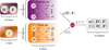 |
Fig. 1 Scheme of the emulator implemented in this work. The system’s ODE describing the ISM chemical network (Sect. 2.1) is emulated via the DeepONet formalism (Sect. 2.2) by splitting the dependence i) from the initial conditions (T, and densities n of each chemical species, i.e. e−, H−, H, H+, He, He+, He++, H2, and |

2.3 Data-set generation
The data used to train and test sets for our models were produced using KROME following the model described in Sect. 2.1. KROME3 (Grassi et al. 2014) is a Python interface that generates the fortran code to solve an input chemical model. The associated ODE system is evolved in time by adopting a fifth-order version of LSODES (Hindmarsh 2019), an implicit, robust, multi-step, iterative4 solver that takes advantage of the sparsity of the Jacobian matrix contracted with the chemical fluxes. For the gas number density, n, and initial temperature, T, we randomly sampled5 64 points in the log-spaced range −2 ≤ log(n/cm−3) ≤ 3.5 and log(20) ≤ log(T/K) ≤ 5.5, respectively, by extracting the points within the variables range. Similarly, the initial fractions of each species ni/n are log-sampled in 512 bins in the range6 −6 ≤ log(ni/n) < 0; we added constraints to ensure that the total hydrogen and helium abundances are close to primordial and that global charge neutrality is respected.
The radiation field, F, is composed of ten energy bins for the photons (see Table 1) and treated as follows7. For a full generalization, each component of the incident flux, Fi, should be treated similarly to the other inputs (n, ni, and T); that is, by randomly extracting the value in a pre-established range. However, this approach would likely generate a completely non-physical spectrum in the vast majority of cases: difference between contiguous Fi would be unbound; for instance, a fully random spectrum might contain He ionizing photons and have a negligible flux in the Habing (1968) band (6.0–13.6 eV). Furthermore, the sampling of Fi should be as refined as the one for the relative abundances, which would increase the size of the dataset and make it harder to load it efficiently in the GPU memory.
Therefore, we adopted the following method. First, we generated 64 flux values Fi in any of the bins in a range Fi ∊ [10−15, 10−5]eV cm−2 s−1 Hz−1. Then, we extracted a flux value in the adjacent bin such that |log(Fi/Fi±1)| ≤ 0.15. In this way, the stochasticity of the incoming flows is maintained, without having completely non-physical spectra. In this way, we substantially reduced the size of the dataset, making it possible to refine the sampling of the initial conditions on the fractions. We note that imposing such a constraint for the flux is somewhat similar to the selection of a continuity prior in spectral energy density fitting when exploring non-parametric star formation rate histories by allowing for burstiness (Tacchella et al. 2020; Ciesla et al. 2024).
The time evolution was evaluated in 16 random uniformly sampled points in the range of 0 ≤ t/kyr ≤ 1. In total, the training set comprises 30% of the dataset and the remaining 70% is used for on-the-fly (during the training) validation, totaling 644 245 094 ≃ 6.4 × 10⁸ points. A summary of the adopted parameters is provided in Table 2.
Summary of the properties used to generate the training set for this work.
3 Results
Here, we present the results of our emulator. We start by checking the precision of the model on the training set and validating it outside the training data range (Sect. 3.1), then showcasing the emulator on a physically relevant case of study (Sect. 3.2). Finally, we make a comparison with other tools aimed at solving ISM photo-chemistry (Sect. 3.3).
In this work, each model is trained for a total of 5 × 10⁴ epochs on a single NVIDIA A100 GPU (40GB), for approximately ≃4.34 GPU hrs per each chemical output (temperature and species); namely, for a total of ≃43.39 GPUhrs for the full set.
3.1 Model testing and validation
For the testing, we assessed the robustness of our results by comparing them against a subset of the KROME-generated data, excluded from the training phase. We start our analysis by showing (in Fig. 2) the results from DeepONet versus KROME in the prediction versus true plane, visualized via a bi-dimensional probability distribution function (PDF). We note that in Fig. 2, we also plot the sum of temperatures and all the species normalized via Eq. (4), while individual PDFs are reported in Figs. A.1 and A.2.
For both the normalized version and individual species, the 2D PFDs are strongly peaked around the predicted=true bisector (dashed black line), with a density that decreases by four orders of magnitude already ~0.1 dex away from the true solution. We note that the stripe features seen in the lower left corners of Fig. 2 are due to the sparse sampling of the extrema of the parameter space and is mostly stemming from the summed combination of H, He, and He++ (see Fig. A.2). Qualitatively, this analysis (in particular, the small distance between bisector and PDF peaks in the whole axis) start to reveal the good accuracy of the predictions as a function of the physical ranges of density and temperature (see Table 2).
Quantitative, a summary of the accuracy is provided in Table 3, which reports the performance in terms of relative errors defined as:
 (5)
(5)
where xtrue represents values computed with KROME and xpred indicates predictions made by our model. Table 3 shows that the quantitative representation of error distribution for all species has mean relative errors of less than 3%, with a median below 2% and a 90% quantile under 6%.
To visualize such a benchmark, in Fig. 3, we plot the PDF of the relative errors for T and all ni. All the PDFs are peaked around ∆r ~ 10−2, with the exception for the error distribution of neutral hydrogen, which presents a peak at higher values, but still less than ∆r ~ 10−1 (i.e. 10%). In most cases, each PDF resembles a Gaussian, which thus can be characterized by its width; the typical width of the distribution can be expressed in terms of standard deviation and, on average, it is approximately σ ≃ 1.3 in log(∆r) space. Thus, a typical error of 0.05% = 10−3.3 ≲ ∆r ≲ 10−0.7 ≃ 0.2 can be expected for each species, for the adopted ≃4.34 GPUhrs of training.
Considering that the training for each species can be performed independently, with the idea that when coupling with a simulation, it is possible and relatively straightforward to use the ∆r PDF (as Fig. 3) as a guideline to seek which species can benefit from further training (as is likely the case with neutral hydrogen here). Moreover, it is important to identify the incidence of outliers, which can be defined as cases with a large relative error greater than, for instance, ∆r > 1. With the current training, such outliers constitute approximately 10−6 % of the total, as can be qualitatively inferred from the rapid drop of the PDF in Fig. 2. This implies, for instance, that in a numerical simulation with ~106 finite elements, a few outliers are likely to affect the results every ~100 time step. For the coupling with numerical simulations such outliers should be prevented (see e.g. Galligan et al. 2019). This can be prevented by simply furthering the training (e.g. with an additional training phase using a second order optimizer, such as L-BFGS). More precisely, an anomaly detector (Pang et al. 2021) can be used, which should be coupled directly with the DeepONet structure. This method will be explored in a future work.
To have a practical idea of the accuracy and performance of the emulator and to validate our model, we illustrate the evolution of chemical species up to 1 kyr for a couple of single set of initial conditions. We can check two different examples. In the first scenario (see the left panel of Fig. 4), the initial conditions include a total gas density of n = 104 cm−3, a temperature of T = 103 K, and a (nearly negligible) photon flux intensity of G = 10−1 G0. The second scenario (right panel of Fig. 4) features n = 102 cm−3, T = 106 K, and G = G0.
We note that these examples act as a test since the evaluation has been done at times, t, which are different with respect to the 16 linearly sampled data points included in the training set. Moreover, both scenarios can be taken as validations, since some species have initial condition outside the training and testing range, namely, in the first case, the gas number density is n = 104 cm−3, while in the second, it is T = 106 K (Table 2).
The results are presented in Fig. 4, where T and each ni are plotted as a function of t. The solid lines report the outcomes computed using the KROME software, while the dashed lines illustrate the predictions from our DeepONet emulator. The overall evolution is accurately captured by our model as seen by the small, namely, ≲ 0.1 dex, distance between the DeepONet and KROME solutions, with errors that tend to decrease at higher times (t ≃ 1 kyr). For the second example, some larger discrepancies are present in the early stages (up to approximately 1 yr) for He; this inaccuracy reflects the fact that the error distribution of He is among the worst (see Fig. 3), namely, ∆r peaks at 10−1.7. Furthermore, we recall that the t training set is extracted from the linearly spaced range of 0 to 1 kyr; thus, the sampling of the data is expected to be lower at early times. These two facts combined can lead to larger errors in the prediction phase.
Indeed, adopting a linear sampling of the training space in the time domain implies a better sampling at high t, thus explaining why the errors seems to decrease with increasing t for most of the species in both examples. Moreover, it is important to note that our emulator captures the sharp turns of some species very well. For instance, in the case of He++ (in the left panel) and  (in the right panel), both feature a numerical gradient of about 10 order of magnitude at t ~ 10 yr, hinting at the fact that our method does not suffer too much from the stiffness of the system.
Errors are small despite the initial density and temperature exceeding the maximum values in the training set (Table 2), indicating that the model not only interpolates the training data, but also seems to gain a good understanding of the influence of initial conditions (the sensors) on the evolution operator. In general, the problem of extrapolating the solutions of neural operators is complex to quantify. Zhu et al. (2023) meticulously analyzed the capability of DeepONet to extrapolate solutions, also proposing experimental methods to enhance the adaptability of trained models to receive unexpected inputs, namely, ones that are beyond the initial dataset. As shown in Fig. 4, our model seems to generalize quite well within a range about half a dex (both for n and T) outside the initial conditions covered by the training set; this can serve as a safety insurance if, for instance, a model reaches an unexpected input value during a numerical simulation. This ability to extrapolate outside the range of initial conditions worsens further away from the limits of the training set. For instance, the accuracy decreases by a factor of 10 if we take an initial T ≃ 107.5 K, that is, with respect to the upper bound of the training dataset, going beyond (by a factor of 2) the normalized log space (see Sect. 2.2).
However, the above discussion does not apply to time extrapolation. In general, it is more challenging for the operator to extrapolate in the time domain. This is primarily due to the nonlinear structure of the ODEs system, which may present sharp turns at late times; thus, it is not included in the testing set for a particular combination of initial conditions. In principle, it is possible to enhance the time extrapolation capability of Deep-Onet by increasing the number of sensors (Lu et al. 2021, in particular, see Sect. 12.1 in the supplementary material). Possibly, a more cost-effective approach for longer time integration would consist of concatenating the solution of the emulator, using the prediction in the first time step as initial conditions for the second iteration and so on, thereby exploiting the fact that no explicit time dependence is present in the photo-chemical network. However, it is unclear how such a concatenation would affect the error propagation and we leave this analysis for a future work.
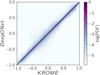 |
Fig. 2 Predicted vs. true test for the DeepONet model. Logarithmic densities for each ion (H, H+, …) and the temperature (T) are normalized in the full dataset range (Table 2) and summed (y, see Eq. (4)) for both the true value from KROME and the predicted value from Deep-ONet. The image shows the 2D probability distribution function (PDF) of the summed dataset and it is normalized such that the maximum is 1 to better appreciate the dynamical range. To guide the eye, we have added a dashed black line to mark the KROME = DeepONet region. See Fig. A.2 for the same diagnostic for individual ions. |
Quantitative summary of the distribution of relative errors, i.e. for the temperature and each chemical species emulated we report the mean relative error (MRE) and the quantiles of the relative errors for 50% (median), 75%, and 90% of the testing cases.
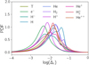 |
Fig. 3 PDF of the relative error (∆r) for the testing set. Each output from the emulator (T and density for each species) is shown independently, with the color-code indicated in the legend. The PDFs are computed using a testing set of ≃2 × 10⁷ of points. |
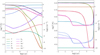 |
Fig. 4 Examples of the time (t) evolution of temperature (T) and the density (n, see the legend) of all the species in the chemical network. The solid lines represent the solutions computed using KROME, while the dashed lines depict the predictions of our models, with each line being a single solution from the emulator. In the left (right) panel the gas number density is n = 104 cm−3 (initial temperature is T = 106 K), namely, outside the range of the training dataset (see Table 2). |
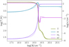 |
Fig. 5 Photo-dissociation region (PDR) benchmark. Temperature (T, right axis) and density of main hydrogen species (H, H+, and H2, left axis) profiles as a function of column density (N) obtained for an impinging radiation flux of 10 G0 propagating in a Z = Z⊙ slab (see Sect. 3.2 for details of the model). Solid lines represent the numerical solutions computed with KROME at equilibrium (t ~ 1 Kyr), dashed lines represent the solution predicted by the emulator. Note: each point in the profile at a given N is treated independently by the emulator. |
3.2 Photo-dissociation region benchmark
For a physically relevant benchmark, we simulated a photo-dissociation region (PDR, see Wolfire et al. 2022 for a review), similarly to the test presented in the photoionization code comparison study from Röllig et al. (2007). Adopting a planar geometry, we took a slab of gas with constant gas density n = 102 cm−3 and a maximum column density of N = 5 × 1021 cm−2. We assumed a constant metallicity Z = Z⊙ with solar abundances (Asplund et al. 2009) and linearly scaled the dust content with the solar value. We set an input radiation field with the spectral shape of a black body of a temperature, T = 3 × 10⁵ K; namely, with the intention of mimicking a massive star that is able to efficiently ionize up to He+. Its intensity is normalized by setting the flux in the Habing band to G = 10 G0, where G0 = 1.6 × 10⁻³ erg cm−2 s−1 is the average Milky Way value (Habing 1968). Here, the radiation field has ten frequency bins: one for each of the photo-chemical reaction included in the chemical network (see Sect. 2.1). We split the slab in optically thin cells and allow for the radiation to propagate trough the slab assuming an infinite speed of light; as the radiation propagates, it is absorbed by dust and gas, whereby the chemical composition and temperature is evolved until equilibrium (t ~ 1 kyr) by KROME. We note that the incident spectrum of the photon (an attenuated black body) can, in principle, be significantly different with respect to the one used for the training; namely, the constrained extraction of the fluxes (see Sect. 2.3).
In Fig. 5, we show the temperature and the main hydrogen ion and molecule profiles as a function of the column density, N. It is important to recall that the profiles do not represent a single solution of the system of ODEs, but a collection of different solutions evaluated at the same t by adopting different attenuation for the incident radiation field, which yield a different local radiation field F and, thus, different thermodynamic conditions. The dashed lines representing the predictions of our emulator reproduce well the general trend of the numerical solution from KROME (solid lines), with errors typically of the order of 7% in the ionized (N ≲ 1018.5 cm−2) and molecular (N ≳ 1019.5 cm−2) regions. However, we see a larger discrepancy in the transition between the ionized and PDR region (N ~ 1019.3 cm−2), on the order of 30%; namely, with errors that are generally larger than expected from the testing (see Sect. 3.1).
From a numerical point of view, we can interpret such a discrepancy as follows. As noted by Lu et al. (2021, in particular see the supplementary material, Sect. 18 therein) DeepONet respects (by constrution) the Holder condition, which in our case translates to:
 (6)
(6)
where 𝒞 is a positive scalar and pa and pb are two different sets of initial conditions and photon fluxes. The Holder condition (Eq. (6)) implies that the solutions predicted by DeepONet tend to be smooth with respect to changes in the initial data, making it more difficult to predict discontinuities. Stating it differently, if the training set is not sampling a region of input parameters with large variations of the outputs finely enough, the emulator will tend to average out the predictions. A general discussion is more complex, as this feature is due to the phenomenon of neural network smoothness (Jin et al. 2020). This discrepancy can likely be ameliorated by having a finer sampled training set in the discontinuity region and/or increasing the architecture size to improve the expressivity.
From a PDR modeling point of view, we note that the discrepancy at the ionized-neutral interface is compatible with the differences between the various photoionization codes adopted in the post-benchmark comparison from (Röllig et al. 2007, see in particular the top panel of Fig. 11 therein). Such differences are due different implementations and assumptions regarding the photo-chemical rates in the various codes. Thus, we can consider as a minor issue the discrepancy we find between Deep-ONet and the reference KROME solution. Furthermore, adopting a finer grid of initial conditions sampling the ionized-neutral transition and/or expanding the depth of the neural network (currently, six layers have been adopted) should ameliorate the issue.
3.3 Comparisons with other models
In Branca & Pallottini (2023), physics-informed neural networks (PINN) were adopted to emulate a photo-chemical network that is very similar to the one in the present; with respect to the results from Branca & Pallottini (2023), DeepONet achieves a typical accuracy that is about 10 times better, with a computational training cost that is about 40 times lower. We consider this to be a stark improvement for the performance; however, training the DeepONet requires pre-computation of a dataset. In principle, this can be expensive (in this case, only ≃ 100 CPUhr are actually used), while PINNs are completely data-independent. The observed performance disparity between the neural operator and the PINN can be attributed to the following factors. The efficacy of the PINN method is known to heavily rely on the initial conditions set selected during training. In Branca & Pallottini (2023), we developed a technique to generalize for initial conditions that are unknown at the time of training, by elevating the initial condition to a vector. However, there is no strict theoretical guarantee for the feasibility of this approach and we hypothesize that this limitation is the primary cause of the lower accuracy observed in the PINN, compared to DeepONet when trained for an equivalent duration. In addition to enhanced precision, with respect to the PINN from Branca & Pallottini (2023), a significant advancement would be the possibility of having an explicit dependency on incident radiation. This allows the DeepONet model to be effectively coupled with real-time radiative transfer codes, for instance, in following the evolution of local molecular clouds (Decataldo et al. 2020). Instead, in order to use DeepONet to study the formation and evolution of galaxies in the EoR (Pallottini et al. 2022), variations of the metallicity should be allowed and we plan to explore this in a future work.
In Grassi et al. (2022) and Sulzer & Buck (2023), the capabilities of autoencoders to compress a large chemical network (29 chemical species and 224 reactions) into a latent space were explored; subsequently, the latent variables were evolved using both standard stiff ODE integrator (Grassi et al. 2022) and a neural ODE approach (Sulzer & Buck 2023). The chemical network in these works is larger than the one adopted here (9 chemical species and 52 reactions; see Sect. 2.1). This difference naturally favors the compression approach; however, in these models, the evolution of temperature, dependence of the evolution on the initial total density, dependence of the coupling coefficient on temperature, and the impact of incident radiation are not considered. Furthermore, another limitation is given by the fact that the size of the latent space is fixed a priori. Keeping these differences in mind, compared to the present work the overall accuracy is worse by a factor of ~20 for the case of direct numerical integration in the latent space (Grassi et al. 2022, i.e. as for Branca & Pallottini 2023), but similar to the case where the neural ODE solver is implemented (Sulzer & Buck 2023).
Furthermore, comparing our results on the PDR with those obtained by CHEMULATOR (Holdship et al. 2021), we obtained a better agreement with the numerical solutions, for instance, a ∆r ≃ 7% compared to a ∆r ≃ 20% errors with respect to the reference solutions; however, it is notable that our chemical network contains a lower number of species and reactions, compared to the system with 30 species and 330 reactions adopted in Holdship et al. (2021). Moreover, in addition to smaller relative errors, a notable difference is in the regularity of our solutions, which are much smoother than those from CHEMULATOR. Such a difference is likely driven by the fact that CHEMULATOR is a purely data driven method. Instead, DeepONet also tries to reproduce the map between the initial conditions and the family of solutions of the ODE system (Lu et al. 2021), since it is an application of the UAT for operators (Chen & Chen 1995). This implies DeepONet is expected to follow the Holder condition (see Eq. (6)).
Finally, we note that the time required to make ≃2 × 10⁷ predictions is about 25.36 CPU seconds. Compared to the 3240.0 CPUs needed by KROME, this gives us an approximate speed-up of = 128, effectively making the chemical-evolution task inexpensive. Such a speed-up with respect to a traditional stiff ODE solver is of the same order of magnitude as the ones reported in Branca & Pallottini (2023) and Grassi et al. (2022). However, it is lower by a factor of ~10 than the one found in Sulzer & Buck (2023), in the case where the integration in the latent space is replaced by a linear fitting function. In the case of CHEMULATOR (Holdship et al. 2021), the authors reported a remarkable speed-up factor of 5 × 10⁴ compared to UCLCHEM (Holdship et al. 2017), which significantly surpasses our results. However, drawing a direct comparison is challenging as UCLCHEM and KROME are very distinct codes, each employing different underlying ODEs solvers and with a different usage case in numerical simulation, namely, with post-processing and on-the-fly usage, respectively, in most instances. Indeed, even with the low 128× speed-up obtained by DeepONet, substituting a traditional ODE solver with our method would effectively make inexpensive the thermo-chemical step in a numerical simulation.
4 Conclusions
In this work, we develop a non-equilibrium photo-chemical emulator to cure the computational bottlenecks that hinder the inclusion of detailed chemistry in state-of-the-art astrophysical simulations. This study pioneers the exploration of a neural operator, specifically, DeepONet, for this application.
We adopted the ISM photo-chemical network from Bovino et al. (2016, with 9 species and 52 reactions) that has been used for studies of Giant Molecular Cloud (GMC, Decataldo et al. 2019) and galaxies (Pallottini et al. 2019). We trained DeepONet with dataset generated by solving the ISM photochemistry via KROME (Grassi et al. 2014), by adopting for the initial conditions a gas number density, n, temperature, T, and fractions of each species, ni/n, that are sampled in log-spaced range −2 ≤ log(n/cm−3) ≤ 3.5, log(20) ≤ log(T/K) ≤ 5.5, and −6 ≤ log(ni/n) < 0, respectively. Furthermore, we allowed for a varying radiation field, F, composed of 10 energy bins for the photons, with each sampled in the range of Fi ∊ [10−15, 10−5] eV cm−2 s−1 Hz−1 by imposing a continuity prior; such that [log(Fi/Fi±1)] ≤ 0.15 in adjacent bins. Time was sampled in the 0 ≤ t/kyr ≤ 1 range and the full dataset contains ≃ 6.4 × 10⁸ models. The model was tested and validated both with idealized and physically motivated scenarios, and the key results can be summarized as follows:
Our deep learning model for ISM chemistry has given results that are both accurate (relative error ∆r ~ 10−2) and fast to compute (~128 times faster than a traditional solver) with a relatively low training time (total of ~eq43.4 GPUhrs);
By employing DeepONet, we have realized significant enhancements over previous models, particularly when compared with physics-informed neural networks (PINNs, Branca & Pallottini 2023), with our approach showing a higher accuracy (10×) at a reduced computational cost (40×) during the training phase, alongside a streamlined model parameter framework;
A critical innovation is the integration of arbitrary radiation fields, a considerable leap beyond the constraints of traditional chemical emulators. This adaptability to diverse radiation fields is a substantial breakthrough, enabling more accurate modeling in scenarios where radiation significantly influences astrophysical dynamics, such as in the dynamics of GMC (e.g. Decataldo et al. 2020).
In summary, the present approach seems to surpass the performance of PINNs (Branca & Pallottini 2023) in terms of precision and incorporates a direct dependence on radiation fields, outperforming autoencoder-based methods (Grassi et al. 2022) for problems with relatively small chemical networks (i.e. 9 species and 52 reactions).
However, a few limitations affect the current emulation. For instance, we observed larger discrepancies in the transition between ionized and photo-dissociation regions (PDRs), which could be attributed to DeepONet’s inherent inclination towards smooth, continuous solutions. While such discrepancy is of the same order of magnitude as the difference between different photoionization codes (Röllig et al. 2007), this characteristic may influence the model’s efficacy in predicting abrupt transitions in chemical profiles. Our model shows robustness in extrapolating beyond the initial condition (density and temperature) ranges, indicating its potential applicability across a broader spectrum of astrophysical scenarios; however, the model’s extrapolation capabilities are limited in the temporal domain. This issue can be mitigated by iteratively applying the trained model multiple times, effectively extending its predictive reach. To couple it effectively in a numerical simulation, the propagation of the error should be carefully tested and outliers (rare, large deviations with respect to the average errors) should be prevented; for instance, via anomaly detection or further training. An avenue for future enhancement might involve the exploration of multi-output DeepONet models, which could potentially offer increased precision by harnessing inherent conservation laws within the system, thereby addressing the challenges associated with sharp transitions between various astrophysical conditions.
In conclusion, the present work implies a significant leap forward in the modeling of ISM chemistry, offering an emulator with a good balance of precision, versatility, and computational efficiency. However, addressing the challenges of better managing transitions between distinct regions and refining the model’s capability in handling extrapolation beyond the training domain remains a vital area for future research. Such endeavors not only promise to refine the existing model but also pave the way for more comprehensive simulations of complex astrophysical processes.
Acknowledgements
We gratefully acknowledge computational resources of the Center for High Performance Computing (CHPC) at SNS. We acknowledge the CINECA award under the ISCRA initiative, for the availability of high performance computing resources and support from the Class C project PINNISM HP10CB99R0 (PI: Branca). Supported by the Italian Research Center on High Performance Computing Big Data and Quantum Computing (ICSC), project funded by European Union – NextGenerationEU – and the National Recovery and Resilience Plan (NRRP) – Mission 4 Component 2 within the activities of Spoke 3 (Astrophysics and Cosmos Observations)
Appendix A Individual predicted versus true tests
In this Appendix, we report the individual predicted vs true analysis for the temperature (Fig. A.1) and all ions (Fig. A.2) included in the photo-chemical network. The plot scheme is the same one adopted for the composed analysis shown in Fig. 2 in the main text.
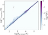 |
Fig. A.1 Predicted vs true data shown as 2D PDF for the temperature with respect to KROME data. The black dashed line is the bisector and represent a region without dicrepancy between data and predictions. |
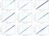 |
Fig. A.2 Predicted vs true data for all the species with respect to KROME data. The colorbar is given in Fig. A.1. |
References
- Abadi, M., Agarwal, A., Barham, P., et al. 2015, TensorFlow: Large-Scale Machine Learning on Heterogeneous Systems, https://www.tensorflow.org/ [Google Scholar]
- Asplund, M., Grevesse, N., Sauval, A. J., & Scott, P. 2009, ARA&A, 47, 481 [NASA ADS] [CrossRef] [Google Scholar]
- Bakes, E. L. O., & Tielens, A. G. G. M. 1994, ApJ, 427, 822 [NASA ADS] [CrossRef] [Google Scholar]
- Bezanson, J., Edelman, A., Karpinski, S., & Shah, V. B. 2017, SIAM Rev., 59, 65 [Google Scholar]
- Bovino, S., Grassi, T., Capelo, P. R., Schleicher, D. R. G., & Banerjee, R. 2016, A&A, 590, A15 [NASA ADS] [CrossRef] [EDP Sciences] [Google Scholar]
- Branca, L., & Pallottini, A. 2023, MNRAS, 518, 5718 [Google Scholar]
- Caselli, P., & Ceccarelli, C. 2012, A&A Rev., 20, 56 [NASA ADS] [CrossRef] [Google Scholar]
- Cen, R. 1992, ApJS, 78, 341 [NASA ADS] [CrossRef] [Google Scholar]
- Chen, T., & Chen, H. 1995, IEEE Transactions on Neural Networks, 6, 911 [CrossRef] [Google Scholar]
- Chen, T., & Guestrin, C. 2016, KDD ’16: Proceedings of the 22nd ACM SIGKDD International Conference on Knowledge Discovery and Data Mining, 785 [CrossRef] [Google Scholar]
- Ciesla, L., Ilbert, O., Buat, V., et al. 2024, A&A, in press, https://doi.org/10.1051/0004-6361/202348091 [Google Scholar]
- Cybenko, G. 1989, Math. Control Signals Syst., 2, 303 [Google Scholar]
- Danehkar, A., Oey, M. S., & Gray, W. J. 2022, ApJ, 937, 68 [NASA ADS] [CrossRef] [Google Scholar]
- Decataldo, D., Pallottini, A., Ferrara, A., Vallini, L., & Gallerani, S. 2019, MNRAS, 487, 3377 [Google Scholar]
- Decataldo, D., Lupi, A., Ferrara, A., Pallottini, A., & Fumagalli, M. 2020, MNRAS, 497, 4718 [NASA ADS] [CrossRef] [Google Scholar]
- Ferland, G. J., Chatzikos, M., Guzmán, F., et al. 2017, Rev. Mex. Astron. Astrofis., 53, 385 [NASA ADS] [Google Scholar]
- Galli, D., & Palla, F. 1998, A&A, 335, 403 [NASA ADS] [Google Scholar]
- Galligan, T. P., Katz, H., Kimm, T., et al. 2019, arXiv e-prints [arXiv: 1981.81264] [Google Scholar]
- Glorot, X., & Bengio, Y. 2010, in Proceedings of Machine Learning Research, Proceedings of the Thirteenth International Conference on Artificial Intelligence and Statistics, eds. Y. W. Teh & M. Titterington, Chia Laguna Resort, Sardinia, Italy, 9, 249 [Google Scholar]
- Glover, S. C. O., & Abel, T. 2008, MNRAS, 388, 1627 [NASA ADS] [CrossRef] [Google Scholar]
- Glover, S. C. O., Federrath, C., Mac Low, M. M., & Klessen, R. S. 2010, MNRAS, 404, 2 [Google Scholar]
- Gnedin, N. Y., & Hollon, N. 2012, ApJS, 202, 13 [Google Scholar]
- Grassi, T., Bovino, S., Schleicher, D. R. G., et al. 2014, MNRAS, 439, 2386 [Google Scholar]
- Grassi, T., Nauman, F., Ramsey, J. P., et al. 2022, A&A, 668, A139 [NASA ADS] [CrossRef] [EDP Sciences] [Google Scholar]
- Gray, W. J., Oey, M. S., Silich, S., & Scannapieco, E. 2019, ApJ, 887, 161 [NASA ADS] [CrossRef] [Google Scholar]
- Habing, H. J. 1968, Bull. Astron. Inst. Netherlands, 19, 421 [Google Scholar]
- Hennigh, O., Narasimhan, S., Nabian, M. A., et al. 2020, arXiv e-prints [arXiv:2012.07938] [Google Scholar]
- Heyl, J., Butterworth, J., & Viti, S. 2023, MNRAS, 526, 404 [NASA ADS] [CrossRef] [Google Scholar]
- Hindmarsh, A. C. 2019, Astrophysics Source Code Library [record ascl:1905.021] [Google Scholar]
- Hirashita, H., & Ferrara, A. 2002, MNRAS, 337, 921 [NASA ADS] [CrossRef] [Google Scholar]
- Holdship, J., Viti, S., Jiménez-Serra, I., Makrymallis, A., & Priestley, F. 2017, AJ, 154, 38 [NASA ADS] [CrossRef] [Google Scholar]
- Holdship, J., Viti, S., Haworth, T. J., & Ilee, J. D. 2021, A&A, 653, A76 [NASA ADS] [CrossRef] [EDP Sciences] [Google Scholar]
- Jin, P., Lu, L., Tang, Y., & Karniadakis, G. E. 2020, Neural Networks, 130, 85 [CrossRef] [Google Scholar]
- Jura, M. 1975, ApJ, 197, 575 [NASA ADS] [CrossRef] [Google Scholar]
- Katz, H. 2022, MNRAS, 512, 348 [NASA ADS] [CrossRef] [Google Scholar]
- Katz, H., Galligan, T. P., Kimm, T., et al. 2019, MNRAS, 487, 5902 [NASA ADS] [CrossRef] [Google Scholar]
- Kim, J.-G., Kim, W.-T., & Ostriker, E. C. 2018, ApJ, 859, 68 [NASA ADS] [CrossRef] [Google Scholar]
- Kingma, D. P., & Ba, J. 2014, arXiv e-prints [arXiv: 1412.6980] [Google Scholar]
- Kumar, A., & Fisher, R. T. 2013, MNRAS, 431, 455 [NASA ADS] [CrossRef] [Google Scholar]
- Li, Z., Kovachki, N., Azizzadenesheli, K., et al. 2020, arXiv e-prints [arXiv:2010.08895] [Google Scholar]
- Lu, L., Jin, P., & Karniadakis, G. E. 2019a, arXiv e-prints [arXiv:1910.03193] [Google Scholar]
- Lu, L., Meng, X., Mao, Z., & Karniadakis, G. E. 2019b, arXiv e-prints [arXiv: 1907.04502] [Google Scholar]
- Lu, L., Jin, P., Pang, G., Zhang, Z., & Karniadakis, G. E. 2021, Nat. Mach. Intell., 3, 218 [CrossRef] [Google Scholar]
- Lu, L., Meng, X., Cai, S., et al. 2022, Comp. Methods Appl. Mech. Eng., 393, 114778 [CrossRef] [Google Scholar]
- Lundberg, S. M., Erion, G. G., & Lee, S.-I. 2018, arXiv e-prints [arXiv: 1802.03888] [Google Scholar]
- Lupi, A. 2019, MNRAS, 484, 1687 [NASA ADS] [CrossRef] [Google Scholar]
- Maio, U., Dolag, K., Ciardi, B., & Tornatore, L. 2007, MNRAS, 379, 963 [NASA ADS] [CrossRef] [Google Scholar]
- Mao, Z., Lu, L., Marxen, O., Zaki, T. A., & Karniadakis, G. E. 2021, J. Comput. Phys., 447, 110698 [NASA ADS] [CrossRef] [Google Scholar]
- Obreja, A., Macciò, A. V., Moster, B., et al. 2019, MNRAS, 490, 1518 [CrossRef] [Google Scholar]
- Obreja, A., Arrigoni Battaia, F., Macciò, A. V., & Buck, T. 2024, MNRAS, 527, 8078 [Google Scholar]
- Olsen, K. P., Pallottini, A., Wofford, A., et al. 2018, Galaxies, 6, 100 [NASA ADS] [CrossRef] [Google Scholar]
- Pallottini, A., Ferrara, A., Bovino, S., et al. 2017, MNRAS, 471, 4128 [NASA ADS] [CrossRef] [Google Scholar]
- Pallottini, A., Ferrara, A., Decataldo, D., et al. 2019, MNRAS, 487, 1689 [Google Scholar]
- Pallottini, A., Ferrara, A., Gallerani, S., et al. 2022, MNRAS, 513, 5621 [NASA ADS] [Google Scholar]
- Pang, G., Shen, C., Cao, L., & van den Hengel, A. 2021, ACM Comput. Surv., 54, 1 [Google Scholar]
- Prasthofer, M., De Ryck, T., & Mishra, S. 2022, arXiv e-prints [arXiv:2205.11404] [Google Scholar]
- Rackauckas, C., Innes, M., Ma, Y., et al. 2019, arXiv e-prints [arXiv:1902.02376] [Google Scholar]
- Robinson, D., Avestruz, C., & Gnedin, N. Y. 2024, MNRAS, 528, 255 [NASA ADS] [CrossRef] [Google Scholar]
- Röllig, M., Abel, N. P., Bell, T., et al. 2007, A&A, 467, 187 [Google Scholar]
- Rosdahl, J., Katz, H., Blaizot, J., et al. 2018, MNRAS, 479, 994 [NASA ADS] [Google Scholar]
- Shen, S., Madau, P., Guedes, J., et al. 2013, ApJ, 765, 89 [NASA ADS] [CrossRef] [Google Scholar]
- Smith, B. D., Bryan, G. L., Glover, S. C. O., et al. 2017, MNRAS, 466, 2217 [NASA ADS] [CrossRef] [Google Scholar]
- Springel, V., Pakmor, R., Zier, O., & Reinecke, M. 2021, MNRAS, 506, 2871 [NASA ADS] [CrossRef] [Google Scholar]
- Sulzer, I., & Buck, T. 2023, arXiv e-prints [arXiv:2312.06015] [Google Scholar]
- Tacchella, S., Forbes, J. C., & Caplar, N. 2020, MNRAS, 497, 698 [Google Scholar]
- Theuns, T., Leonard, A., Efstathiou, G., Pearce, F. R., & Thomas, P. A. 1998, MNRAS, 301, 478 [NASA ADS] [CrossRef] [Google Scholar]
- Trebitsch, M., Dubois, Y., Volonteri, M., et al. 2021, A&A, 653, A154 [NASA ADS] [CrossRef] [EDP Sciences] [Google Scholar]
- Ucci, G., Ferrara, A., Pallottini, A., & Gallerani, S. 2018, MNRAS, 477, 1484 [Google Scholar]
- Vallini, L., Pallottini, A., Ferrara, A., et al. 2018, MNRAS, 473, 271 [NASA ADS] [CrossRef] [Google Scholar]
- Van Rossum, G., & Drake, F. L. 2009, Python 3 Reference Manual (Scotts Valley, CA: CreateSpace) [Google Scholar]
- Wakelam, V., Herbst, E., Loison, J. C., et al. 2012, ApJS, 199, 21 [Google Scholar]
- Webber, W. R. 1998, ApJ, 506, 329 [NASA ADS] [CrossRef] [Google Scholar]
- Wolfire, M. G., Vallini, L., & Chevance, M. 2022, ARA&A, 60, 247 [NASA ADS] [CrossRef] [Google Scholar]
- Zhu, M., Zhang, H., Jiao, A., Karniadakis, G. E., & Lu, L. 2023, Comput. Methods Appl. Mech. Eng., 412, 116064 [CrossRef] [Google Scholar]
- Ziegler, U. 2016, A&A, 586, A82 [NASA ADS] [CrossRef] [EDP Sciences] [Google Scholar]
The reaction rates are taken from Bovino et al. (2016): reactions 1 to 31, 53, 54, and from 58 to 61 in their Tables B.1 and B.2, photo-reactions P1 to P9 in their Table 2.
We adopted the default errors for KROME, i.e. relative and absolute tolerances are fixed at 10−4 and 10−20 respectively.
In principle, the validity of the UAT for operators does not depend on the distribution of the training data. For DeepONet, a uniform random sampling is generally adopted in the literature; see Prasthofer et al. (2022, in particular, theorem 3.1) for an example of non-uniform data sampling.
Note that the limit on the fraction is applied only to the initial conditions, because of the chemical evolution individual species are allowed to be as low down to nmin = 10−10cm−3.
Note that in KROME, the radiation field is a pure input, i.e. individual fluxes Fi are not directly evolved by the system. In the typical usage case, KROME is coupled to a numerical simulation, the former provides the opacities, the latter include the radiative transfer modules for the evolution of Fi (e.g. Pallottini et al. 2019).
All Tables
Quantitative summary of the distribution of relative errors, i.e. for the temperature and each chemical species emulated we report the mean relative error (MRE) and the quantiles of the relative errors for 50% (median), 75%, and 90% of the testing cases.
All Figures
|
Fig. 1 Scheme of the emulator implemented in this work. The system’s ODE describing the ISM chemical network (Sect. 2.1) is emulated via the DeepONet formalism (Sect. 2.2) by splitting the dependence i) from the initial conditions (T, and densities n of each chemical species, i.e. e−, H−, H, H+, He, He+, He++, H2, and |
| In the text | |
|
Fig. 2 Predicted vs. true test for the DeepONet model. Logarithmic densities for each ion (H, H+, …) and the temperature (T) are normalized in the full dataset range (Table 2) and summed (y, see Eq. (4)) for both the true value from KROME and the predicted value from Deep-ONet. The image shows the 2D probability distribution function (PDF) of the summed dataset and it is normalized such that the maximum is 1 to better appreciate the dynamical range. To guide the eye, we have added a dashed black line to mark the KROME = DeepONet region. See Fig. A.2 for the same diagnostic for individual ions. |
| In the text | |
|
Fig. 3 PDF of the relative error (∆r) for the testing set. Each output from the emulator (T and density for each species) is shown independently, with the color-code indicated in the legend. The PDFs are computed using a testing set of ≃2 × 10⁷ of points. |
| In the text | |
|
Fig. 4 Examples of the time (t) evolution of temperature (T) and the density (n, see the legend) of all the species in the chemical network. The solid lines represent the solutions computed using KROME, while the dashed lines depict the predictions of our models, with each line being a single solution from the emulator. In the left (right) panel the gas number density is n = 104 cm−3 (initial temperature is T = 106 K), namely, outside the range of the training dataset (see Table 2). |
| In the text | |
|
Fig. 5 Photo-dissociation region (PDR) benchmark. Temperature (T, right axis) and density of main hydrogen species (H, H+, and H2, left axis) profiles as a function of column density (N) obtained for an impinging radiation flux of 10 G0 propagating in a Z = Z⊙ slab (see Sect. 3.2 for details of the model). Solid lines represent the numerical solutions computed with KROME at equilibrium (t ~ 1 Kyr), dashed lines represent the solution predicted by the emulator. Note: each point in the profile at a given N is treated independently by the emulator. |
| In the text | |
|
Fig. A.1 Predicted vs true data shown as 2D PDF for the temperature with respect to KROME data. The black dashed line is the bisector and represent a region without dicrepancy between data and predictions. |
| In the text | |
|
Fig. A.2 Predicted vs true data for all the species with respect to KROME data. The colorbar is given in Fig. A.1. |
| In the text | |
Current usage metrics show cumulative count of Article Views (full-text article views including HTML views, PDF and ePub downloads, according to the available data) and Abstracts Views on Vision4Press platform.
Data correspond to usage on the plateform after 2015. The current usage metrics is available 48-96 hours after online publication and is updated daily on week days.
Initial download of the metrics may take a while.