| Issue |
A&A
Volume 691, November 2024
|
|
|---|---|---|
| Article Number | A224 | |
| Number of page(s) | 12 | |
| Section | Numerical methods and codes | |
| DOI | https://doi.org/10.1051/0004-6361/202451789 | |
| Published online | 15 November 2024 | |
Deep operator neural network applied to efficient computation of asteroid surface temperature and the Yarkovsky effect
1
School of Astronomy and Space Science, Nanjing University,
Nanjing
210023,
China
2
Key Laboratory of Modern Astronomy and Astrophysics in Ministry of Education, Nanjing University,
Nanjing
210023,
China
3
Shanghai Astronomical Observatory, Chinese Academy of Sciences,
Shanghai
200030,
China
★ Corresponding author; This email address is being protected from spambots. You need JavaScript enabled to view it.
Received:
4
August
2024
Accepted:
24
September
2024
Abstract
Surface temperature distribution is crucial for thermal property-based studies about irregular asteroids in our Solar System. While direct numerical simulations could model surface temperatures with high fidelity, they often take a significant amount of computational time, especially for problems for which temperature distributions are required to be repeatedly calculated. To this end, the deep operator neural network (DeepONet) proves a powerful tool due to its high computational efficiency and generalization ability. In this work, we apply DeepONet to the modeling of asteroid surface temperatures. Results show that the trained network is able to predict temperature with an accuracy of ~1% on average, while the computational cost is five orders of magnitude lower, enabling thermal property analysis in a multidimensional parameter space. As a preliminary application, we analyzed the orbital evolution of asteroids through direct N- body simulations embedded with an instantaneous Yarkovsky effect inferred by DeepONet-based thermophysical modeling. Taking asteroids (3200) Phaethon and (89433) 2001 WM41 as examples, we show the efficacy and efficiency of our AI-based approach.
Key words: methods: numerical / celestial mechanics / minor planets, asteroids: general
© The Authors 2024
 Open Access article, published by EDP Sciences, under the terms of the Creative Commons Attribution License (https://creativecommons.org/licenses/by/4.0), which permits unrestricted use, distribution, and reproduction in any medium, provided the original work is properly cited.
This article is published in open access under the Subscribe to Open model. This email address is being protected from spambots. You need JavaScript enabled to view it. to support open access publication.
1 Introduction
Surface temperature distribution is an important property of asteroids, and the base for a wide range of thermal- related studies, such as the Yarkovsky and Yarkovsky–O’Keefe– Radzievskii–Paddack (YORP) effects. The prediction of surface temperature distributions requires thermophysical modeling that solves heat conduction equations by incorporating both the shape of the asteroid and various thermal and physical properties.
Generally, thermal models are classified into simple thermal models that consider the heat conduction of spherical asteroids and more comprehensive thermophysical models that consider a broader range of factors (Delbó et al. 2015). Simple models include the standard thermal model (STM) (Lebofsky et al. 1986), the fast rotating model (FRM) (Lebofsky & Spencer 1989), the near-Earth asteroid thermal model (NEATM) (Harris 1998), and the night emission simulated thermal model (NESTM) (Wolters & Green 2009). STM and FRM are rarely used at present (see more details about these models in Delbó & Harris 2002 and Delbó et al. 2015). More sophisticated thermophysical models have been introduced by Lagerros (1996a,b); Lagerros (1997, 1998), Delbó (2004), Čapek & Vokrouhlický (2005), and Rozitis & Green (2011).
To obtain temperature distribution over the surface of an irregular asteroid, a polyhedral shape model is commonly used that represents the topography with triangular facets. While some studies consider transverse heat conduction to establish three-dimensional (3D) equations, such as the models used by Davidsson & Rickman (2014), Xu et al. (2022) and Nakano & Hirabayashi (2023), most of the time it is sufficient to solve one-dimensional (1D) heat conduction equations for each facet (Delbó et al. 2015). Direct numerical simulation based on a finite-difference technique is a high-precision method for solving heat conduction equations, but it requires a high computation cost because of iterative calculations performed on a large number of time-space grids (Delbó et al. 2015).
High-fidelity thermophysical models are widely applied in the inversion of asteroids’ physical properties that are essential for understanding their formation and evolution. For example, an asteroid’s size is related to its collision history (Bottke et al. 2005), the thermal inertia related to the surface material composition (Delbó et al. 2007), and so on. The inversion can be realized by comparing modeled thermal emission to the observations. For example, the thermal inertia of the asteroid (101955) Bennu has been studied in detail by combining the thermophysical models with the mid-infrared observations (Müller et al. 2012; Emery et al. 2014; Yu & Ji 2015). The properties of asteroid (1862) Apollo were constrained by combining the thermophysical model with light curve, thermal-infrared, and radar observations (Rozitis et al. 2013). Moreover, with the determined thermal properties, it is possible to calculate the orbital drift caused by Yarkovsky effect and rotational acceleration from the YORP effect. By fitting them to the observed data, we can further determine axis ratios, effective diameter, geometric albedo, thermal inertia, and bulk density (Rozitis et al. 2013), such as the studies about the asteroid (6489) Golevka (Chesley et al. 2003), the asteroid (152563) 1992 BF (Vokrouhlický et al. 2008), Bennu (Chesley et al. 2014), and the asteroid (3200) Phaethon (Hanuš et al. 2018). In particular, Golevka is the first asteroid that has been confirmed to have orbital drift caused by Yarkovsky effect (Chesley et al. 2003). Yarkovsky and YORP effects are also critical for the assessment of impact risk (Farnocchia et al. 2013; Farnocchia & Chesley 2014), dynamical spreading of the asteroid families (Vokrouhlický et al. 2010; Hanuš et al. 2013), and so on (see more details from Bottke et al. 2006 and Vokrouhlický et al. 2015).
Studies about the Yarkovsky effect usually utilize analytical thermal models (also called linear models) proposed by Vokrouhlický (1998a,b, 1999) due to the high computational burden associated with numerical simulations (Rozitis & Green 2012; Xu et al. 2022). Linear models consider spherical asteroids with relatively uniform surface temperature distributions that compute simply and fast, but the tradeoff is precision. However, analytical models may cause additional errors, leading to low-level precision. Chesley et al. (2014) studied the orbital evolution of Bennu from 2000 to 2136 under the influence of Yarkovsky effect calculated under three methods: a transverse acceleration in a simple form, a linear model, and a nonlinear model based on Čapek & Vokrouhlický (2005). Similarly, Farnocchia et al. (2021) studied the ephemeris and impact hazard assessment of Bennu utilizing three methods, including the linear model and two nonlinear models proposed by Čapek & Vokrouhlický (2005) and Rozitis & Green (2011), respectively. Xu et al. (2022) compared the drift caused by the Yarkovsky effect of 34 irregular asteroids from an analytical model and a numerical simulation, showing that it is overestimated by 16%–36% with the analytical model. For those high-precision problems, numerical simulations for thermophysical models are necessary.
When assessing orbital evolution under the Yarkovsky effect, it is common to first generate a lookup table of the Yarkovsky force against the orbital elements to avoid solving the thermophysical models at each step of orbit integration. If the orbit is frozen, an interpolation function based on true anomaly angle suffices (Chesley et al. 2003; Xu et al. 2022). When the evolution of the orbit is incremental, it is an accepted way to compute the Yarkovsky force from the linearized expansion about a central orbit with semimajor axis a0 and eccentricity e0 and further generate a lookup table about a0 + δa, e0 + δe, and a true anomaly angle (Chesley et al. 2014; Farnocchia et al. 2021). However, the linear approximation is no longer applicable when there are significant changes in the orbital elements. Without linear approximation, it is impossible to obtain orbital evolution of asteroids through direct 3D N -body simulations embedded with a precise Yarkovsky effect because of the high computation cost of producing the surface temperature at each step with a direct numerical simulation.
To resolve the bottleneck of computational cost in direct numerical simulations, we aim to propose a method that can efficiently produce surface temperature distributions, and thus enable the study of long-term orbital evolutions of irregular asteroids under the precise Yarkovsky effect. In recent years, physics-informed neural networks (PINNs) (Raissi et al. 2019) have had successful applications in a variety of problems because of their efficiency in solving ordinary differential equations (ODEs) and partial differential equations (PDEs) (Cai et al. 2020; Martin & Schaub 2022a,b; Zobeiry & Humfeld 2021; Mathews & Thompson 2023; He et al. 2021; Laghi et al. 2023). The basic model of PINN is a fully connected neural network, embedding physical equations in the loss function. Being equation driven is a prominent feature of PINN. However, it requires one to repeatedly train the network when the boundary conditions or parameters of the problem’s ODEs or PDEs change. Thus, the training cost of PINN may not be less than that of traditional numerical simulations. For the current problem discussed in this work, there are many factors influencing the surface temperature distribution of asteroids. A neural network with greater generalization ability is required to address this problem. In this regard, we have adopted the deep operator neural network (DeepONet) developed by Lu et al. (2021), which can handle this kind of problem with variations in boundary conditions and model parameters. It has been successfully applied in various cases (Garg et al. 2022; He et al. 2023; Branca & Pallottini 2024).
The following content shows how we (i) explore the feasibility of DeepONet as a unified model for computing the surface temperature distribution of asteroids with varying physical parameters, and (ii) explore the possibilities of DeepONet in solving the problems about the parameter space analysis of Yarkovsky acceleration and the orbital evolution of asteroids under the precise Yarkovsky effect.
2 Thermophysical model and the Yarkovsky effect
In this work, the thermophysical model developed by Čapek & Vokrouhlický (2005) has been adopted, which considers the selfshadowing effect between facets, while neglecting self-heating. It should be mentioned that the method based on neural network can be applied to more complex models, such as the model proposed by Rozitis & Green (2011).
2.1 Thermophysical model
2.1.1 Heat conduction equation
In thermophysical models, the asteroid is regarded as polyhedron consisting of a large number of triangular facets. When the dimension of facets are sufficiently large, the lateral heat conduction can be neglected. Thus, only the perpendicular heat conduction is taken into account. To obtain the global surface temperature, the 1D heat conduction equation is solved for each facet (see more detail in Lagerros 1996a, Čapek & Vokrouhlický 2005, and Rozitis & Green 2011). The 1D heat conduction equation reads
 (1)
(1)
where ρ represents the surface density, C is the specific heat capacity, and κ is the thermal conductivity. For simplicity, the parameters (ρ, C, κ) are assumed to be independent from the time, depth, and temperature.
To make the solution unique, boundary conditions have to be applied. One is the surface boundary condition derived from conservation of energy and the other one is about the constancy of temperature at large depths, given by
 (2)
(2)
where ϵ is the emissivity, σ is the Stefan–Boltzmann constant, and AB is the Bond albedo. The parameter s indicates whether the facet is illuminated by the Sun. s = 1 when the facet is illuminated and s = 0 when it is unilluminated. ψ represents the cosine function of the solar elevation angle and it can be calculated from cosine law ψ = a ⋅ b/|a||b|, where a and b, respectively, represent the direction of the Sun and the outward-pointing unitary normal vector of the facet. It should be noted that s and ψ depend on both the rotation of asteroid and the topography. In particular, s = 0 if ψ ≤ 0 (horizon shadows) or the facet is shadowed by other facets (projected shadows). F⊙ is the incident solar radiation flux determined by F⊙ = S⊙/r2, where r is the heliocentric distance of the asteroid and S⊙ is the solar constant.
For convenience, Eqs. (1)–(2) need to be normalized as follows (Lagerros 1996a):
 (3)
(3)
and
 (4)
(4)
with the normalized variables  given by

where E(t) = sψ is defined in the range [0,1]. The coefficient, Φ, is referred to as the thermal parameter (see Eq. (7) in Spencer et al. 1989), given by

where  is called the surface thermal inertia, ω is the rotational angular velocity of the asteroid,
  is called the skin depth, and
  is called the characteristic temperature (Lagerros 1996a; Rozitis & Green 2011; Yu & Ji 2015).
2.1.2 Numerical simulation
The first step is to compute the solar radiation flux function about the time, E(t) = sψ. As was mentioned above, s and ψ change periodically as the asteroid rotates, meaning that E(t) is also a periodic function of time. Therefore, it is required to determine E(t) in the first period. The calculation of ψ is based on cosine law.
The time-consuming step is to make shadow tests. There are two types of shadows: horizon shadows and projected shadows. The horizon shadows can be determined from the sign (plus or minus) of ψ, while the projected shadows are usually difficult to calculate. This can be regarded as a ray–triangle intersection problem, in which the triangle is the facet of interest and the ray can be reasonably approximated as the sunlight passing through the center of gravity of the facet. Each facet needs to be tested against the remaining facets and the test process needs to be repeated when the position of the Sun changes. To save computation time, it is common practice to store the outcomes and retrieve the shadow results from a lookup table (Čapek & Vokrouhlický 2005; Rozitis & Green 2011). In this work, the Möller–Trumbore algorithm has been adopted (Tomas & Ben 1997).
To solve the 1D heat conduction equation, we need to divide continuous variables into a set of space-time grids, where the ith grid of depth is denoted by  and the j-th grid of time is denoted by
  . As a result, Eqs. (3–4) are discretized into the following form (Rozitis & Green 2011):
 (5)
(5)
and
 (6)
(6)
The surface boundary condition can be solved to determine  from the known
  by taking advantage of Newton-Raphson iterative algorithm.
The surface of an asteroid could form a static temperature distribution in an inertial frame, meaning that the temperature is invariant at the subsolar point after a full rotation. This provides a cycle termination condition to solve Eqs. (5)–(6).
The numerical simulation of determining the global surface temperature of an asteroid is an N3 problem, whose scale is determined by the number of facets, steps of iterations, and the numbers of the time grid. It needs to be repeatedly solved once any model parameter changes, and thus takes a large amount of computational resources.
2.2 Yarkovsky effect
The Yarkovsky effect includes diurnal and seasonal components (Bottke et al. 2006). The diurnal Yarkovsky effect maximizes when the spin axis of the asteroid is perpendicular to its orbital plane and the seasonal effect maximizes when the spin axis of the asteroid is in its orbit plane.
For the diurnal effect, the hotter spot on the surface of an asteroid is shifted away from the subsolar point into the afternoon because of thermal inertia. These regions will reradiate more energy into space, meaning that more momentum departs from the hotter part of the asteroid as the infrared photon carries away momentum equal to E /c, where E is the energy and c is the speed of light. This mechanism causes the Yarkovsky force in the transverse and radial directions. As for the seasonal effect, its timescale is equal to the orbital period of the asteroid. The hemisphere facing the Sun is hotter during the revolution, causing an along-track Yarkovsky force as resistance to the movement in a low-eccentricity orbit. This effect is only important for those asteroids with relatively high thermal inertia (Rozitis & Green 2012).
The first step to determine the Yarkovsky force is to compute the surface temperature of the asteroid with the numerical simulation mentioned above. Then, the Yarkovsky force is determined by assuming that the emitted radiation follows Lambert’s law, given by (Spitale & Greenberg 2001; Bottke et al. 2006)
 (7)
(7)
where n is the external unitary normal vector of the facet and S is the area of the facet. In practical simulations, the integral can be approximated as the sum of the force on each facet.
3 Deep operator neural network (DeepONet)
Numerical simulation, as is discussed in Sect. 2, is an accurate approach for producing the surface temperature distribution of an asteroid. However, its inefficiency will become an obstacle for many projects, especially in situations requiring repeated computation of the surface temperature. In this regard, the neural network provides a powerful tool with less computational cost and a greater ability to generalize. In this study, the deep operator neural network (DeepONet), developed by Lu et al. (2021), has been adapted to address the problem.
3.1 Architecture of DeepONet
DeepONet is a deep neural network for learning operators, based on the universal approximation theorem of the operator (Chen & Chen 1995; Lu et al. 2021). The operator about a function of u in space, C(K1), is denoted by G, and the corresponding function in another function space, C(K2), can be regarded as G(u). This mapping relation, u → G(u), can be approximated by the networks by inputting u and outputting G(u). If we take y as any variable in the domain of function, G(u), G(u)(y) is a real number, and the mapping relation y → G(u)(y) can also be approximated by networks. These two parts constitute Deep- ONet: branch networks for u → G(u) and trunk networks for y → G(u)(y). In fact, such an approximation can be regarded as the process of learning potential nonlinear operators from physical equations (see more details in Lu et al. 2021).
In the present work, the solar radiation flux function, E, is the key function and the thermal parameter, Φ, is the key parameter of boundary conditions for heat conduction equation. When the two factors are determined, the surface temperature distribution is determined by solving the 1D heat conduction equation. As was mentioned in the previous section, the flux function, E, varies with the position of the Sun, and thus the external unitary normal vector of the facet or the shadow of the facet may change. In addition, the thermal parameter, Φ, is related to thermal parameters, including the surface thermal inertia, Γ (it is a function of the surface density, ρ, the specific heat capacity, C, and the thermal conductivity, κ), rotational angular velocity, ω, Bond albedo, AB, the heliocentric distance, r, and so on.
We denote the solution of heat conduction equation by

where G(E, Φ) is the operator to be learned. The operator is different from the original version of DeepONet. In practice, E is suggested to be represented discretely. A convenient way is to employ the function values evaluated at a sufficiently large but finite number of locations, ![Mathematical equation: $[E({\bar t_1}),E({\bar t_2}),...,E({\bar t_m})]$](/articles/aa/full_html/2024/11/aa51789-24/aa51789-24-eq21.png) , and the variables,
, and the variables, ![Mathematical equation: $[{\bar t_1},{\bar t_2},...,{\bar t_m}]$](/articles/aa/full_html/2024/11/aa51789-24/aa51789-24-eq22.png) , are called sensors. Φ is a real number that can be directly input into the network. Therefore, the input of the branch networks are the functions evaluated at discrete locations,
, are called sensors. Φ is a real number that can be directly input into the network. Therefore, the input of the branch networks are the functions evaluated at discrete locations, ![Mathematical equation: $[E({\bar t_1}),E({\bar t_2}),...,E({\bar t_m})]$](/articles/aa/full_html/2024/11/aa51789-24/aa51789-24-eq23.png) , and the real number, Φ.
, and the real number, Φ.
The solution of heat conduction equation is a 2D matrix about  and
and  . We are only concerned with the surface temperature at a certain time for a facet, meaning the temperature at
  and
and  is required, so it is appropriate to reduce the range of variables for better approximation and more convenient training. In practice, grids of depth,
 ![Mathematical equation: $[{\bar z_1},{\bar z_2},...,{\bar z_n}]$](/articles/aa/full_html/2024/11/aa51789-24/aa51789-24-eq28.png) , are chosen to be the inputs of the trunk networks.
, are chosen to be the inputs of the trunk networks.
In summary, we can see that branch networks are used to learn the operator associated with parameters of dynamical model and the trunk network is used to learn the mapping relation of inputs and outputs associated with the heat conduction equation. Based on this concept, a variety of similar problems can be addressed by taking advantage of DeepONet.
There are n variables in the input of trunk network, meaning that the output also includes n components. Thus, it is necessary to match the numbers of output with branch networks. Two approaches can be employed: one is to repeat the results of the branch network n times and the other one is to repeat the input locations ![Mathematical equation: $[E({\bar t_1}),E({\bar t_2}),...,E({\bar t_m})]$](/articles/aa/full_html/2024/11/aa51789-24/aa51789-24-eq29.png) and parameter “Φ” n times. The two approaches are equivalent. In this work, the second one was taken. The input after repetition reads
and parameter “Φ” n times. The two approaches are equivalent. In this work, the second one was taken. The input after repetition reads

The schematic architecture of DeepONet adapted for the problem considered in this work is shown in Fig. 1, where the trunk and branch networks are presented in Fig. 2. As one of the improvements to the original DeepONet, two branch networks were used to separately learn the operators related to the radiation flux function, E, and the thermal parameter, Φ. E is the input into branch neti and Φ is the input into branch net2 . The Hadamard product between the output of them become the input of SELayer. As a second improvement to the original DeepONet, we introduced the attention mechanism in the SELayer, further improving the accuracy of approximation (Vaswani et al. 2017; Lu et al. 2021). The original SELayer is called squeeze-and- excitation networks (Hu et al. 2018). The output is the product between the importance weights and the corresponding channels of the previous feature map. Its essence is to learn the influence of each channel on the final output, and thus achieve a better feature extraction (Hu et al. 2018; Woo et al. 2018; Wang et al. 2020). In this work, SELayer is modified by introducing a fully connected architecture, and another fully connected layer is appended for residual operation following the “excitation” step. The modified SELayer is applied to branch net1, branch net2, and trunk net.
The output from SELayer is denoted as bk and the output from trunk net is tk, with k changing from 1 to p. The final output is the dot product between them with a bias, b0,
 (8)
(8)
The trunk network applies the activation functions, LeakyReLU (Maas 2013), in the last layer, and thus we can regard the adapted DeepONet network as consisting of two branch networks and a trunk network as a full trunk network, where the weights in the last layer are parameterized by branch networks.
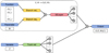 |
Fig. 1 Architecture of the modified DeepONet adopted in this work. The network learning the operator G : (E, Φ) → G(E, Φ) includes three inputs, the function, E, the parameter, Φ. E is presented as some discrete locations with m elements sampled on |
![Mathematical equation: $[{\bar t_1},{\bar t_2},...,{\bar t_m}]$](/articles/aa/full_html/2024/11/aa51789-24/aa51789-24-eq18.png)

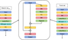 |
Fig. 2 Detailed architectures of branch net1 , branch net2, and SELayer adopted in this work, where FC is the fully connected layer and BN is the batch normalization layer. The input of branch net1(2) experiences the initial feature extraction through a fully connected layer and then carries out the feature amplification by 4(2) SELayer. Trunk net is similar but it should be noted that there is an activation function before the output. SELayer in this work is a modified squeeze-and-excitation layer specially for fully connected architecture. |
3.2 Dataset and training
DeepONet is a data-driven neural network, and thus a high-quality training dataset is crucial for its performance. The dataset can be produced with random pairs of E and Φ through direct numerical simulations. Lu et al. (2021) has provided two function spaces: Gaussian random field (GRF) and Chebyshev polynomials. In this study, we use mean-zero GRF denoted as

where the covariance kernel, kl(x1, x2), is the radial-basis function, called Gaussian kernel in GRF. l is the length scale determining the smoothness of the function (a larger l corresponds to a smoother u), (x1, x2) are feature vectors, and ||x1 − x2|| represents the Euclidean distance between these two vectors.
The random functions generated from GRF theoretically extend over large ranges, but E is controlled in the range [0,1], as was mentioned in Sect. 2.1.1. Therefore, we rescaled the random functions by applying the sigmoid function 1/(1 + e−x). In order to ensure the completeness of the function space, we performed translation operations on partial random functions before inputting them into the sigmoid function, meaning that the actual transformation formula is denoted as 1/(1 + e−(x+d)), where d represents the distance of translation along the y-axis. This step helps to maintain endmost values (such as in the range of (0.9,1), (0,0.1), …). Then, the new random functions can be sampled on sensors ![Mathematical equation: $\left[ {{{\bar t}_1},{{\bar t}_2}, \ldots ,{{\bar t}_m}} \right]$](/articles/aa/full_html/2024/11/aa51789-24/aa51789-24-eq33.png) to obtain the discrete input solar radiation flux functions.
to obtain the discrete input solar radiation flux functions.
The dataset used in this work consists of 16 000 functions without translation, 8000 functions with d = −2.5, 8000 functions with d = −3, 6000 functions with d = −6, 2000 functions with d = −10, and 6000 functions with d = 6. There is a corresponding random ¢ for each function. By feeding them into the heat conduction equation and performing numerical simulation, we obtain the corresponding temperature distributions that form the overall dataset. The temperatures computed from these functions fall within different ranges between 0 and 1, with some having very small differences between the maximum and minimum values. The network may not be very sensitive when learning from these data. So it is important to preprocess the data before training. Z-score normalization is an effective method, reading

where X is the original data, Z is the data after transformation, µX is the mean of X, and σX is the standard deviation of X. The primary purpose of Z-score is to standardize data of different magnitudes into a single scale and the data measured uniformly by Z-score can ensure comparability among them.
The loss function in this work is the mean square error (MSE) between the temperature from the dataset and the output from DeepONet, and the optimization algorithm is the adaptive moment estimation method (Adam). To avoid the issue of the loss function oscillating widely and converging slowly, we employed the learning rate decay approach. The learning rate in training diminishes with increasing epochs, reading

where lr0 is the initial learning rate, ep is the current epoch, and epmax is the total epoch. Table 1 summarizes the settings for the training process. With the dataset prepared, the training time is about 10 minutes.
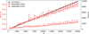 |
Fig. 3 Time cost of DeepONet and traditional numerical simulation as a function of number of facets. The red line consisting of error bars centered around circles represents the time cost required by DeepONet in GPU and the red line consisting of error bars centered around squares represents the time cost required by DeepONet in CPU. The black line is the time cost required by traditional numerical simulation. |
Parameter settings of training.
4 Results
We used two indicators to assess the performance of the trained DeepONet: the cost of computation time and the level of accuracy.
4.1 Cost of computation time
A short inference time is one of the most prominent advantages of a neural network over numerical simulation. Additionally, the strong generalization ability of neural networks supports practical applications to a variety of problems after training. Under a given hardware, the inference time of neural networks depend on the batch size of the input and the intrinsic complexity of the problem.
In order to make a direct comparison of the time cost, both the DeepONet algorithm and the direct numerical approach (difference algorithm) were adopted to produce the surface temperature for a test sphere-shaped asteroid with the number of facets varying in the range of [500,20 000]. Figure 3 shows the time consumption of three methods as a function of the number of facets. For each set of temperature calculations, we performed DeepONet’s computation over 20 times using both GPU and CPU. The average computation time with GPU and CPU is shown by hollow circles and hollow squares, respectively, and the maximum and minimum times are marked in the form of error bar. Regarding numerical simulations, we pre-calculated the temperatures for a large number of different facets and obtained the average time cost per facet. The results, shown in Fig. 3, represent such an average value multiplied by the number of computations. All of the computations were performed on a personal computer1 and under the environment of Python 3.8.
As is shown in Fig. 3, DeepONet plus GPU proves to be the most efficient strategy. For an asteroid with 20 000 facets, DeepONet plus GPU can produce the global temperature distribution in less than 0.06 seconds, over 160000 times faster than the numerical simulation (at least five orders of magnitude improvement in terms of computational efficiency). DeepONet plus CPU is also significantly faster than numerical methods, but has less advantages than the GPU solution with a large number of facets. Furthermore, if we need to compute a large number of global temperature distributions, such as for different asteroids or different parameters, vectorized operations can be further used to ensure that the computation time does not increase linearly with the number of global temperature distributions, because the internal calculations of networks are carried out using matrix operations.
4.2 Performance of accuracy
We have used the example of three asteroids the shape of a sphere, a biaxial ellipsoid (ax = 2ay = 2az), and a triaxial ellipsoid (ax = 2ay = 3az), which can represent widely used convex polyhedral shape models of asteroids. We calculated the global temperature distribution for the different obliquity, β, defined as the angle between the spin axis and the normal vector of the orbital plane, and the different thermal parameter, Φ. Figure shows the result. The mean absolute error (MAE) stands for the relative deviation of temperature, ∆T/T, between DeepONet and the numerical simulation.
The overall error is maintained at a relatively low level of less than 2%. We noticed certain patterns in the error distribution: (a) the error decreases, in general, as β increases. This indicates a more accurate temperature in the high-temperature areas, since the number of high-temperature facets increases and the highest temperature is also higher when β is larger; (b) the error decreases as the thermal parameter increases, which similarly implies a more accurate temperature in the high-temperature areas, since the overall temperature distribution becomes more uniform, the highest temperature decreases, but the number of high-temperature facets increases when Φ is larger (also meaning that the surface thermal inertia or the rotational angular velocity is larger). The conclusion is helpful for calculating the Yarkovsky force, because the influence on the force is greater in high-temperature regions (F is directly related to T4).
Irregular asteroids require the consideration of projected shadows between two arbitrary facets, resulting in a more complex radiation flux function. It is a great challenge for the generalization ability of the network. To analyze the accuracy performance of DeepONet on irregular asteroids, we used as examples the dataset of asteroids (21) Lutetia and (8567) 1996 HW1 from the Planetary Data System2. The thermal parameters were assumed to be Φ = 6.4163 and Te = 258.3404 K, calculated by some assumed physical parameters (AB = 0.33, e = 0.9, Γ = 400 J m−2s−1/2K−1, r = 2 au, P = 8.76243 h). These two irregular asteroids contain various degrees of projected shadows: some are the large-scale shadows caused by the concave shape, and some are small-scale shadows due to the local topography, which represent the real situation of most asteroids. Figure 5 shows the comparison between the global temperature distributions of the two asteroids from DeepONet and numerical simulation, with the Sun located in the positive x-axis direction.
The relative errors remain at a low level of less than 1% for the majority of facets. Only a small number of facets have errors around 2%. The projected shadows do have an impact on the computation accuracy, as the errors are slightly larger in the areas with a significant self-shadowing effect, but still within an acceptable range. As for the previous analysis, we also evaluated the MAE of ∆T/T as the functions of β and Φ, which are shown in Fig. 6. The errors are consistent with those shown in Fig. 4, and hence show the strong generalization ability of DeepONet, supporting reliable calculations even with high-complexity input functions.
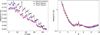 |
Fig. 4 Error between the results from DeepONet and numerical simulation. The panels describe the MAE of ∆T/T as a function of β (left panel) and of Φ (right panel), where the black lines represent the spherical asteroid, the blue lines are the biaxial ellipsoid, and the red lines are the triaxial ellipsoid. The left panels fix Φ = 5 and the right panels fix β = 90°. |
5 Applications
As was mentioned before, the short inference time by using DeepONet makes it possible to solve problems that require a large number of repeated computations of temperature distributions. In this section, we apply DeepONet to two such problems: analysis of the Yarkovsky force in multiparameter space and the orbital evolution of asteroids under the precise Yarkovsky effect.
5.1 Parameter analysis
The temperature distribution and the resulting Yarkovsky force of asteroids are closely related to their physical properties. It is crucial to understand their relationship, which can be applied to exact predictions about how the Yarkovsky force changes with a certain physical parameter (Bottke et al. 2006). In addition, it is beneficial for the problem of parameter inversion of asteroids.
Traditionally, the inversion of an asteroid’s thermal-related properties is performed by minimizing a fitting factor measuring the discrepancy between the radiation flux from simulated temperature distribution and mid-infrared observation data (Müller et al. 2011; Emery et al. 2014; Yu & Ji 2015). Alternatively, when the drift of the orbital semimajor axis is measured, fitting the Yarkovsky effect with variable parameters also leads to the estimation properties (Chesley et al. 2003; Vokrouhlický et al. 2008; Chesley et al. 2014; Hanuš et al. 2018).
Both methods require the exploration of a large parameter space that is usually computationally expensive. Here, we took advantage of DeepONet to make a parameter analysis about Yarkovsky acceleration for a spherical asteroid with 2112 facets. We explored the distributions of transverse and radial Yarkovsky accelerations in the (ρ, C), (β, r) and (R, κ) spaces with a high-resolution ratio (100 × 100). In each space, the remaining parameters were fixed as default values, as is shown in Table 2. It takes a short time to produce distributions of Yarkovsky acceleration in the three parameter spaces. In Sect. 4.1, it is mentioned that using matrix operations instead of iterative methods to compute global temperature distributions under various conditions can greatly reduce time costs. The specific implementation details can be found in the code that we have uploaded to GitHub3. In this case, the computation time for Yarkovsky acceleration in 2D space can be reduced to 8 seconds.
The results, shown in Fig. 7, indicate that: (a) The transverse Yarkovsky acceleration increases with surface density and specific heat capacity, whereas the radial acceleration shows the opposite trend, (b) The Yarkovsky acceleration decreases with increasing heliocentric distance. While the transverse component decreases with increasing obliquity, the radial part shows the opposite trend, (c) Both accelerations decrease with the size of the asteroid. The transverse component increases first and then decreases with thermal conductivity, and the radial component consistently decreases. We note that the dependency also reflects the influence of Φ on the transverse and radial accelerations, which can be understood from the theoretical relationships given in Vokrouhlický et al. (2017):

which provide a first guess for the nonlinear case. These behaviors are also compatible with those found in previous works by Bottke et al. (2006) and Xu et al. (2022).
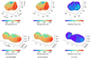 |
Fig. 5 Surface temperatures of two irregular asteroids from DeepONet and the traditional simulation, and the relative errors between them. The top panels are for amain belt asteroid (Lutetia) and the bottom panels are for an Amor-class asteroid (1996 HW1). The left column panels describe the results from DeepONet, the middle column panels are the results from traditional simulation, and the right column panels are relative errors between the two methods. |
Default setting of parameters in parameter space analysis.
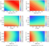 |
Fig. 7 Magnitude of (a) transverse and (b) radial Yarkovsky accelerations produced by DeepONet for a sphere asteroid shown in different parameter spaces, spanned by the specific heat capacity, C, the density, ρ, the distance from the Sun, r, the rotational inclination, β, the radius, R, and the thermal conductivity, κ. For the three situations, except for the two studied parameters, other parameters are fixed. The magnitude of acceleration is shown in the color bar. |
5.2 Orbital evolutions under the Yarkovsky effect
Using the traditional numerical simulations, it is difficult to consider long-term evolution of asteroids under the N-body problem with the precise Yarkovsky effect. Thus, the widely used approach for treating the Yarkovsky effect in the process of discussing orbital evolution is to make a linear approximation (the so-called analytical method) (Vokrouhlický 1998a,b, 1999; Bottke et al. 2006). If irregular asteroids are considered, these errors introduced by linear approximation may be amplified (Xu et al. 2022), resulting in significant deviations. DeepONet enables fast computation of the Yarkovsky force, while maintaining a certain level of accuracy, making it possible to provide in real time a precise Yarkovsky force during the orbital evolution in an N-body system.
We take the near-Earth asteroid (3200) Phaethon and the main-belt asteroid (89433) 2001 WM41 to be representatives.
Their orbital configurations are shown in Fig 8. As the rotation period of the two asteroids is much shorter than their orbital periods, we assumed that the surface temperature distribution reaches a dynamic equilibrium state at any point of their orbits. Therefore, it is possible to obtain an instantaneous Yarkovsky force at each position along the orbit, which is applied to the orbit propagation with an N-body dynamical model including the gravitational perturbations from eight planets and the moon. The results are compared to those obtained from analytical methods (linear models mentioned in Sect. 1).
The shape models and physical parameters of Phaethon and 2001 WM41 are from DAMIT4 (Hanuš et al. 2016a,b). Their polyhedron models are shown in Fig. 9 and their parameters are provided in Table 3. It should be mentioned that some parameters for 2001 WM41 are unknown, and they are taken as hypothetical values. The surface density and bulk density are assumed to be the same. The initial time and evolution time is 2023.9.13.0 and an orbital period of 20000 for Phaethon, and 2024.3.31.0 and an orbital period of 10000 for 2001 WM41. The initial orbital data comes from the Minor Planet Center5.
Because Mercury is considered in the N-body dynamical model, the time step of numerical integration becomes very small, resulting in a staggering number of computation times for the Yarkovsky forces during orbit integration. A precomputed high-precision database is produced and called during numerical propagation. The database is generated based on the position of the Sun. Each position of the Sun is represented by spherical coordinates, r, θ, ϕ, in the asteroid body-fixed coordinate system, where the origin is located at the center of the asteroid, the z-axis is parallel to the spin axis, and the x-axis points to the Sun when the asteroid is on the ascending node between its orbit and equator. The database with 128×128×128 grids is produced in about 8 minutes with the matrix manipulation (the code we have uploaded to GitHub is designed to compute this database). We have verified the accuracy of the database by comparing the short-time orbits propagated with real-time Yarkovsky acceleration calculations and with the database.
Figures 10 and 11 show the orbital evolutions with the Yarkovsky effect developed by the linear model and DeepONet. As for Phaethon, the evolution of semimajor axis is significantly influenced by the Yarkovsky effect, showing visibly different behaviors under different models, even diverging in direction. Without the Yarkovsky effect, the semimajor axis of Phaethon will be larger after 30 000 years compared to its current value (showing outward migration). Both models considering the Yarkovsky effect show that the semimajor axis will be smaller after 30000 years (showing inward migration). However, evolutionary paths under the real-time Yarkovsky force computed by DeepONet and the approximate Yarkovsky force from analytical theory are distinctly different. Regarding the inclination and eccentricity, the evolutionary trends of the three models are qualitatively similar, but also exhibit certain degrees of deviation. For 2001WM41, the influence of Yarkovsky force is relatively small, mainly causing the amplitude of the orbital element oscillation to gradually increase, while the evolution calculated by the three models is nearly identical over 40000 years. The influence of the Yarkovsky force from DeepONet is evidently smaller than that from the analytical model.
The different levels of influences of the Yarkovsky effect upon the orbital evolution of Phaethon and 2001WM41 is related to the characteristics of their orbits. Phaethon is located on a highly eccentric orbit, with a small perihelion distance of 0.14 au. This causes a relatively small Φ and large Te at perihelion, resulting in large surface temperature variation with high temperature at the subsolar point of Phaethon exceeding 1000 K. This translates into a large Yarkovsky force that could cause a significant impact on the orbital evolution. On the other hand, the close encounters to Phaethon with Venus and Earth cause a highly nonlinear dynamical environment that is sensitive to initial conditions. This has been demonstrated by Hanuš et al. (2016a), where each trajectory with a different initial value corresponds to a clone variant. Therefore, the significant differences in the orbital evolution of Phaethon with and without the Yarkovsky effect fundamentally arise from the perturbation (Yarkovsky effect) present in the chaotic dynamical system. Such a relatively significant Yarkovsky effect serves as a “switch” that changes the orbital evolution from one clone to another. Regarding 2001 WM41, it is located in the main belt and the Yarkovsky force is relatively small. Within the timescale of the simulation, it does not play a significant role and is only coupled with N-body perturbations, leading to a slight increase in the oscillating amplitude of orbital elements.
For asteroids like Phaethon in a chaotic dynamical system, there may be significant discrepancies between the actual orbital evolution and the prediction using analytical Yarkovsky models. This is due to the fact that the analytical models are based on the assumption of small temperature variation across the surface and the approximation obtained by Taylor expansion from the nonlinear terms. When the asteroid is very close to the Sun or has specific physical properties, these approximations could lead to significant temperature deviations. Furthermore, if we take into account a chaotic system or an asteroid with an irregular shape, the inaccuracy in the assumption will be further amplified. However, for main-belt asteroids or others located far away from planets or the Sun, the differences are relatively small.
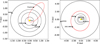 |
Fig. 8 Orbits of Phaethon (left) and 2001 WM41 (right) in the J2000.0 Earth equatorial coordinate system. The yellow points represent the Sun. the black lines are the planet orbits, and the red lines represent the orbits of asteroids. |
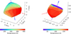 |
Fig. 9 Convex polyhedron shape models and surface temperatures of Phaethon and 2001 WM41 at the initial time. The left panel corresponds to Phaethon and the right panel is for 2001 WM41. The blue arrows represent the direction of the rotation axis and the red arrows represent the direction of the sunlight at the initial time. The surface temperatures are shown in the color bar. |
Thermal and dynamical parameters of Phaethon and 2001 WM41.
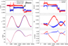 |
Fig. 10 Orbital evolution of Phaethon under different dynamical models (left column panels) and their differences (right panels). The evolutions of the semimajor axis, eccentricity, and inclination are presented in the left column panels, where the gray lines stand for the evolution without the Yarkovsky force, the blue lines represent the evolution with a linear approximation of the Yarkovsky force, and the red lines are for the evolution with the Yarkovsky force produced from DeepONet. |
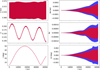 |
Fig. 11 Similar to Fig. 10 but for the orbital evolution of 2001 WM41. The gray line is barely visible due to the fact that it is almost overlapping the other two lines. |
6 Conclusion
In this work, we have explored the possibility of using neural networks to model the surface temperature of asteroids and consider orbit evolutions of asteroids under the precise Yarkovsky effect. We have adapted the deep operator neural network (DeepONet) by adding branch networks to learn which parameters influence the heat conduction equation. Moreover, we have embedded the attention mechanism in the network to achieve better feature extraction. This network can learn the implicit nonlinear operators in the ID heat conduction equation, and thus achieves the goal of solving the equation. With a trained network, we can directly infer the global surface temperature distribution by inputting all facets of an asteroid as a batch.
The simulation results indicate a significant improvement in computational speed compared to the direct numerical simulation. In particular, for an asteroid with 20 000 facets, DeepONet with GPU is about 1.6 × 10⁵ times faster than the traditional numerical method and the increase of computational cost is less steep. We assessed the accuracy of the DeepONet solution by examining errors in temperature with changing obliquity and the thermal parameter. The errors can be controlled below about 2%, averaging about 0.2%. Additionally, two irregular asteroids were taken to test errors in the presence of self-shadowing effect that can complicate the radiation flux function. The results show that the errors in temperature and the Yarkovsky force remain at low levels.
The networks with high computational efficiency and low-level errors are useful for computationally heavy problems, the typical case being the Yarkovsky effect. We tested our model on both parameter space analysis and orbital evolution related to the Yarkovsky effect. Combining a network with matrix computations allows for the rapid calculation of the Yarkovsky force in parameter space, which could largely facilitate any study concerning parameter inversion.
The DeepONet model was also successfully applied in the analysis of orbit evolution. We studied Phaethon and 2001 WM41 in N-body systems under Yarkovsky effects: the former is located in a highly eccentric orbit near Earth, and the latter is in the main belt. Simulation results indicate that the Yarkovsky effect has a significant impact on Phaethon, showing an overall decreasing trend in its semimajor axis, while the effect on 2001 WM41 is relatively weak. Furthermore, we compared the relatively accurate evolution of orbital elements with the results calculated using analytical models, suggesting that the numerical models are the best choice to solve the problems about irregular asteroids, especially Phaethon-like asteroids with large variations in surface temperature, or in a chaotic dynamic system. The adoption of neural network like DeepONet makes the inclusion of precise Yarkovsky effect possible.
We anticipate a broad range of applications for this DeepONet-based thermophysical modeling in analysing problems, such as multidimensional parameter inversion, and long-term orbital evolution under the combination of instantaneous Yarkovsky and YORP effects. A similar AI-based approach can be extended to more complex physical processes, such as the thermophysical modeling of comets.
Acknowledgements
The authors thank Dr. Vokrouhlicky for insightful review comments that helped to significantly improve the manuscript. SJZ wishes to thank Drs. Yining Zhang and Yangbo Xu for helpful discussions about the thermophysical model of asteroids. XS thanks members of the ISSI International Team “Timing and Processes of Planetesimal Formation and Evolution” for inspirational discussions. This work is financially supported by the National Natural Science Foundation of China (Nos. 12073011 and 12233003) and the National Key R&D Program of China (No. 2019YFA0706601).
References
- Bottke, W. F., Durda, D. D., Nesvorny, D., et al. 2005, Icarus, 175, 111 [NASA ADS] [CrossRef] [Google Scholar]
- Bottke, W. F., Vokrouhlický, D., Rubincam, D. P., & Nesvorny, D. 2006, Annu. Rev. Earth Planet. Sci., 34, 157 [CrossRef] [Google Scholar]
- Branca, L., & Pallottini, A. 2024, A&A, 684, A203 [NASA ADS] [CrossRef] [EDP Sciences] [Google Scholar]
- Cai, S., Wang, Z., Chryssostomidis, C., & Karniadakis, G. E. 2020, in ASME 2020 Fluids Engineering Division Summer Meeting collocated with the ASME 2020 Heat Transfer Summer Conference and the ASME 2020 18th International Conference on Nanochannels, Microchannels, and Minichannels, 3: Computational Fluid Dynamics; Micro and Nano Fluid Dynamics, V003T05A054 [Google Scholar]
- Čapek, D., & Vokrouhlický, D. 2005, Dyn. Popul. Planet. Syst., 197, 171 [Google Scholar]
- Chen, T., & Chen, H. 1995, IEEE Trans. Neural Networks, 6, 911 [CrossRef] [Google Scholar]
- Chesley, S. R., Ostro, S. J., Vokrouhlický, D., et al. 2003, Science, 302, 1739 [NASA ADS] [CrossRef] [Google Scholar]
- Chesley, S. R., Farnocchia, D., Nolan, M. C., et al. 2014, Icarus, 235, 5 [NASA ADS] [CrossRef] [Google Scholar]
- Davidsson, B. J. R., & Rickman, H. 2014, Icarus, 243, 58 [NASA ADS] [CrossRef] [Google Scholar]
- Delbó, M. 2004, The Nature of Near-earth Asteroids from the Study of their Thermal Infrared Emission [Google Scholar]
- Delbó, M., & Harris, A. W. 2002, Meteor. Planet. Sci., 37, 1929 [CrossRef] [Google Scholar]
- Delbó, M., Dell’Oro, A., Harris, A. W., Mottola, S., & Mueller, M. 2007, Icarus, 190, 236 [CrossRef] [Google Scholar]
- Delbó, M., Mueller, M., Emery, J. P., Rozitis, B., & Capria, M. T. 2015, Asteroid Thermophysical Modeling (University of Arizona Press) [Google Scholar]
- Emery, J. P., Fernáandez, Y. R., Kelley, M. S. P., et al. 2014, Icarus, 234, 17 [NASA ADS] [CrossRef] [Google Scholar]
- Farnocchia, D., & Chesley, S. R. 2014, Icarus, 229, 321 [NASA ADS] [CrossRef] [Google Scholar]
- Farnocchia, D., Chesley, S. R., Chodas, P. W., et al. 2013, Icarus, 224, 192 [Google Scholar]
- Farnocchia, D., Chesley, S. R., Takahashi, Y., et al. 2021, Icarus, 369, 114594 [NASA ADS] [CrossRef] [Google Scholar]
- Garg, S., Gupta, H., & Chakraborty, S. 2022, Eng. Struct., 270 [Google Scholar]
- Hanuš, J., Broz, M., Durech, J., et al. 2013, A&A, 559, A134 [NASA ADS] [CrossRef] [EDP Sciences] [Google Scholar]
- Hanuš, J., Delbó’, M., Vokrouhlicky, D., et al. 2016a, A&A, 592, A34 [NASA ADS] [CrossRef] [EDP Sciences] [Google Scholar]
- Hanuš, J., Durech, J., Oszkiewicz, D. A., et al. 2016b, A&A, 586, A108 [NASA ADS] [CrossRef] [EDP Sciences] [Google Scholar]
- Hanuš, J., Vokrouhlicky, D., Delbó, M., et al. 2018, A&A, 620, L8 [NASA ADS] [CrossRef] [EDP Sciences] [Google Scholar]
- Harris, A. W. 1998, Icarus, 131, 291 [Google Scholar]
- He, Z. L., Ni, F. T., Wang, W. G., & Zhang, J. 2021, Mater. Today Commun., 28 [Google Scholar]
- He, J. Y., Koric, S., Kushwaha, S., et al. 2023, Comput. Methods Appl. Mech. Eng., 415 [Google Scholar]
- Hu, J., Shen, L., & Sun, G. 2018, in 2018 IEEE/CVF Conference on Computer Vision and Pattern Recognition [Google Scholar]
- Lagerros, J. S. V. 1996a, A&A, 310, 1011 [Google Scholar]
- Lagerros, J. S. V. 1996b, A&A, 315, 625 [NASA ADS] [Google Scholar]
- Lagerros, J. S. V. 1997, A&A, 325, 1226 [NASA ADS] [Google Scholar]
- Lagerros, J. S. V. 1998, A&A, 332, 1123 [Google Scholar]
- Laghi, L., Schiassi, E., De, M., Furfaro, F. R., & Domiziano, M. 2023, Nucl. Sci. Eng., 197, 2373 [NASA ADS] [CrossRef] [Google Scholar]
- Lebofsky, L. A., & Spencer, J. R. 1989, in Asteroids II, 128 (University of Arizona Press) [Google Scholar]
- Lebofsky, L. A., Sykes, M. V., Tedesco, E. F., et al. 1986, Icarus, 68, 239 [NASA ADS] [CrossRef] [Google Scholar]
- Lu, L., Jin, P., Pang, G., Zhang, Z., & Karniadakis, G. E. 2021, Nat. Mach. Intell., 3, 218 [CrossRef] [Google Scholar]
- Maas, A. L. 2013, Rectifier Nonlinearities Improve Neural Network Acoustic Models in ICML2013 [Google Scholar]
- Martin, J., & Schaub, H. 2022a, CeMDA, 134, 13 [NASA ADS] [CrossRef] [Google Scholar]
- Martin, J., & Schaub, H. 2022b, CeMDA, 134, 46 [NASA ADS] [CrossRef] [Google Scholar]
- Mathews, N., & Thompson, B. 2023, Bull. AAS, 55 [Google Scholar]
- Müller, T. G., Durech, J., Hasegawa, S., et al. 2011, A&A, 525, A145 [NASA ADS] [CrossRef] [EDP Sciences] [Google Scholar]
- Müller, T. G., O’Rourke, L., Barucci, A. M., et al. 2012, A&A, 548, A36 [NASA ADS] [CrossRef] [EDP Sciences] [Google Scholar]
- Nakano, R., & Hirabayashi, M. 2023, Icarus, 404, 115647 [NASA ADS] [CrossRef] [Google Scholar]
- Raissi, M., Perdikaris, P., & Karniadakis, G. E. 2019, J. Comput. Phys., 378, 686 [NASA ADS] [CrossRef] [Google Scholar]
- Rozitis, B., & Green, S. F. 2011, MNRAS, 415, 2042 [NASA ADS] [CrossRef] [Google Scholar]
- Rozitis, B., & Green, S. F. 2012, MNRAS, 423, 367 [NASA ADS] [CrossRef] [Google Scholar]
- Rozitis, B., Duddy, S. R., Green, S. F., & Lowry, S. C. 2013, A&A, 555, A20 [NASA ADS] [CrossRef] [EDP Sciences] [Google Scholar]
- Spencer, John, R., Lebofsky, Larry, A., & Sykes, Mark, V. 1989, Icarus, 78, 337 [CrossRef] [Google Scholar]
- Spitale, J., & Greenberg, R. 2001, Icarus, 149, 222 [NASA ADS] [CrossRef] [Google Scholar]
- Tomas, M., & Ben, T. 1997, J. Graph. Tools, 2, 21 [CrossRef] [Google Scholar]
- Vaswani, A., Shazeer, N., Parmar, N., et al. 2017, in Proceedings of the 31st International Conference on Neural Information Processing Systems, NIPS’17 (Red Hook, NY, USA: Curran Associates Inc.), 6000 [Google Scholar]
- Vokrouhlický, D. 1998a, A&A, 335, 1093 [Google Scholar]
- Vokrouhlický, D. 1998b, A&A, 338, 353 [NASA ADS] [Google Scholar]
- Vokrouhlický, D. 1999, A&A, 344, 362 [NASA ADS] [Google Scholar]
- Vokrouhlický, D., Chesley, S. R., & Matson, R. D. 2008, AJ, 135, 2336 [Google Scholar]
- Vokrouhlický, D., Nesvorny, D., Bottke, W. F., & Morbidelli, A. 2010, AJ, 139, 2148 [CrossRef] [Google Scholar]
- Vokrouhlický, D., Bottke, W. F., Chesley, S. R., Scheeres, D. J., & Statler, T. S. 2015, The Yarkovsky and YORP Effects (University of Arizona Press) [Google Scholar]
- Vokrouhlický, D., Pravec, P., Durech, J., et al. 2017, AJ, 153, 270 [CrossRef] [Google Scholar]
- Wang, Q., Wu, B., Zhu, P., et al. 2020, in 2020 IEEE/CVF Conference on Computer Vision and Pattern Recognition [Google Scholar]
- Wolters, S. D., & Green, S. F. 2009, MNRAS, 400, 204 [Google Scholar]
- Woo, S. H., Park, J., Lee, J. Y., & Kweon, I. S. 2018, Comput. Vis. -ECCV 2018, 11211 [Google Scholar]
- Xu, Y. B., Zhou, L. Y., Hui, H. J., & Li, J. Y. 2022, A&A, 666, A88 [NASA ADS] [CrossRef] [EDP Sciences] [Google Scholar]
- Yu, L. L., & Ji, J. H. 2015, MNRAS, 452, 368 [NASA ADS] [CrossRef] [Google Scholar]
- Zobeiry, N., & Humfeld, K. D. 2021, Eng. Applic. Artif. Intell., 101 [Google Scholar]
A laptop equipped with AMD Ryzen 9 6900HX with Radeon Graphics and NVIDIA GeForce RTX 3O7OTi Laptop GPU
All Tables
All Figures
|
Fig. 1 Architecture of the modified DeepONet adopted in this work. The network learning the operator G : (E, Φ) → G(E, Φ) includes three inputs, the function, E, the parameter, Φ. E is presented as some discrete locations with m elements sampled on |
| In the text | |
|
Fig. 2 Detailed architectures of branch net1 , branch net2, and SELayer adopted in this work, where FC is the fully connected layer and BN is the batch normalization layer. The input of branch net1(2) experiences the initial feature extraction through a fully connected layer and then carries out the feature amplification by 4(2) SELayer. Trunk net is similar but it should be noted that there is an activation function before the output. SELayer in this work is a modified squeeze-and-excitation layer specially for fully connected architecture. |
| In the text | |
|
Fig. 3 Time cost of DeepONet and traditional numerical simulation as a function of number of facets. The red line consisting of error bars centered around circles represents the time cost required by DeepONet in GPU and the red line consisting of error bars centered around squares represents the time cost required by DeepONet in CPU. The black line is the time cost required by traditional numerical simulation. |
| In the text | |
|
Fig. 4 Error between the results from DeepONet and numerical simulation. The panels describe the MAE of ∆T/T as a function of β (left panel) and of Φ (right panel), where the black lines represent the spherical asteroid, the blue lines are the biaxial ellipsoid, and the red lines are the triaxial ellipsoid. The left panels fix Φ = 5 and the right panels fix β = 90°. |
| In the text | |
|
Fig. 5 Surface temperatures of two irregular asteroids from DeepONet and the traditional simulation, and the relative errors between them. The top panels are for amain belt asteroid (Lutetia) and the bottom panels are for an Amor-class asteroid (1996 HW1). The left column panels describe the results from DeepONet, the middle column panels are the results from traditional simulation, and the right column panels are relative errors between the two methods. |
| In the text | |
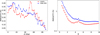 |
Fig. 6 Similar to Fig. 4 but with realistic shapes of irregular asteroids Lutetia and 1996 HW1. |
| In the text | |
|
Fig. 7 Magnitude of (a) transverse and (b) radial Yarkovsky accelerations produced by DeepONet for a sphere asteroid shown in different parameter spaces, spanned by the specific heat capacity, C, the density, ρ, the distance from the Sun, r, the rotational inclination, β, the radius, R, and the thermal conductivity, κ. For the three situations, except for the two studied parameters, other parameters are fixed. The magnitude of acceleration is shown in the color bar. |
| In the text | |
|
Fig. 8 Orbits of Phaethon (left) and 2001 WM41 (right) in the J2000.0 Earth equatorial coordinate system. The yellow points represent the Sun. the black lines are the planet orbits, and the red lines represent the orbits of asteroids. |
| In the text | |
|
Fig. 9 Convex polyhedron shape models and surface temperatures of Phaethon and 2001 WM41 at the initial time. The left panel corresponds to Phaethon and the right panel is for 2001 WM41. The blue arrows represent the direction of the rotation axis and the red arrows represent the direction of the sunlight at the initial time. The surface temperatures are shown in the color bar. |
| In the text | |
|
Fig. 10 Orbital evolution of Phaethon under different dynamical models (left column panels) and their differences (right panels). The evolutions of the semimajor axis, eccentricity, and inclination are presented in the left column panels, where the gray lines stand for the evolution without the Yarkovsky force, the blue lines represent the evolution with a linear approximation of the Yarkovsky force, and the red lines are for the evolution with the Yarkovsky force produced from DeepONet. |
| In the text | |
|
Fig. 11 Similar to Fig. 10 but for the orbital evolution of 2001 WM41. The gray line is barely visible due to the fact that it is almost overlapping the other two lines. |
| In the text | |
Current usage metrics show cumulative count of Article Views (full-text article views including HTML views, PDF and ePub downloads, according to the available data) and Abstracts Views on Vision4Press platform.
Data correspond to usage on the plateform after 2015. The current usage metrics is available 48-96 hours after online publication and is updated daily on week days.
Initial download of the metrics may take a while.