| Issue |
A&A
Volume 684, April 2024
|
|
|---|---|---|
| Article Number | A122 | |
| Number of page(s) | 18 | |
| Section | The Sun and the Heliosphere | |
| DOI | https://doi.org/10.1051/0004-6361/202348768 | |
| Published online | 11 April 2024 | |
Study of solar brightness profiles in the 18–26 GHz frequency range with INAF radio telescopes
I. Solar radius
1
INAF – Cagliari Astronomical Observatory, Via della Scienza 5, 09047 Selargius, CA, Italy
e-mail: This email address is being protected from spambots. You need JavaScript enabled to view it.
2
INAF – Institute of Radio Astronomy, Via Gobetti 101, 40129 Bologna, Italy
3
Istituto Nazionale di Astrofisica (INAF/OAA), Largo Enrico Fermi 5, 50125 Firenze, Italy
4
Los Alamos National Laboratory, Bikini Atoll Rd, Los Alamos, NM 87545, USA
5
ASI – c/o Cagliari Astronomical Observatory, Via della Scienza 5, 09047 Selargius, CA, Italy
6
INAF – Catania Astrophysical Observatory, Via Santa Sofia 78, 95123 Catania, Italy
7
INAF – Turin Astrophysical Observatory, Via Osservatorio 20, 10025 Pino Torinese, TO, Italy
8
INAF – Trieste Astronomical Observatory, Via Giambattista Tiepolo 11, 34131 Trieste, Italy
9
Department of Physics, University of Trieste, Via Alfonso Valerio 2, 34127 Trieste, Italy
10
NRAO – Central Development Laboratory, 1180 Boxwood Estate Rd, Charlottesville, VA 22903, USA
11
ASTRON – The Netherlands Institute for Radio Astronomy, Oude Hoogeveensedijk 4, 7991 PD Dwingeloo, The Netherlands
Received:
28
November
2023
Accepted:
20
January
2024
Abstract
Context. The Sun is an extraordinary workbench, on which several fundamental astronomical parameters can be measured with high precision. Among these parameters, the solar radius R⊙ plays an important role in several aspects, for instance, in evolutionary models. Moreover, it conveys information about the structure of the different layers that compose the solar interior and its atmosphere. Despite the efforts to obtain accurate measurements of R⊙, the subject is still debated, and measurements are puzzling and/or lacking in many frequency ranges.
Aims. We determine the mean, equatorial, and polar radii of the Sun (Rc, Req, and Rpol) in the frequency range 18.1 − 26.1 GHz. We employed single-dish observations from the newly appointed Medicina Gavril Grueff Radio Telescope and the Sardinia Radio Telescope (SRT) in five years, from 2018 to mid-2023, in the framework of the SunDish project for solar monitoring.
Methods. Two methods for calculating the radius at radio frequencies were employed and compared: the half-power, and the inflection point. To assess the quality of our radius determinations, we also analysed the possible degrading effects of the antenna beam pattern on our solar maps using two 2D models (ECB and 2GECB). We carried out a correlation analysis with the evolution of the solar cycle by calculating Pearson’s correlation coefficient ρ in the 13-month running means.
Results. We obtained several values for the solar radius, ranging between 959 and 994 arcsec, and ρ, with typical errors of a few arcseconds. These values constrain the correlation between the solar radius and solar activity, and they allow us to estimate the level of solar prolatness in the centimeter frequency range.
Conclusions. Our R⊙ measurements are consistent with the values reported in the literature, and they provide refined estimates in the centimeter range. The results suggest a weak prolateness of the solar limb (Req > Rpol), although Req and Rpol are statistically compatible within 3σ errors. The correlation analysis using the solar images from the Grueff Radio Telescope shows (1) a positive correlation between solar activity and the temporal variation in Rc (and Req) at all observing frequencies, and (2) a weak anti-correlation between the temporal variation of Rpol and solar activity at 25.8 GHz.
Key words: methods: data analysis / Sun: radio radiation
© The Authors 2024
 Open Access article, published by EDP Sciences, under the terms of the Creative Commons Attribution License (https://creativecommons.org/licenses/by/4.0), which permits unrestricted use, distribution, and reproduction in any medium, provided the original work is properly cited.
This article is published in open access under the Subscribe to Open model. This email address is being protected from spambots. You need JavaScript enabled to view it. to support open access publication.
1. Introduction
The Sun is a mildly active star with an 11-year activity cycle (Gleissberg 1966), emitting radiation in the whole electromagnetic spectrum, from radio to gamma-ray frequencies (e.g. Aschwanden 2004; Landi Degl’Innocenti 2007). It is the closest star for which highly precise fundamental astronomical parameters are known. Of these parameters, the solar radius R⊙, which is usually normalised to the unit distance (1 AU), has been the subject of increasingly accurate measurements and investigations (e.g. Gilliland 1981; Vaquero et al. 2016; Rozelot et al. 2018).
The value of R⊙ allows us to obtain various physical information, such as (1) eclipse computations, (2) the prolateness of the solar limb, and (3) insights into the structure of the different layers in the solar atmosphere. Moreover, determination of the changes in R⊙ provides insights into the physical mechanisms that may cause its variation (e.g. Gilliland 1981; Ribes et al. 1991), enabling a better understanding of (1) the variation in the luminosity and its possible climate effects on the Earth and its environment (e.g. Dansgaard et al. 1975; Stuiver 1980; Hiremath & Mandi 2004; Chapman et al. 2008; Hiremath et al. 2015), and (2) the structure of the solar interior, and the role of the underlying magnetism (e.g. Emilio et al. 2000; Kilic & Golbasi 2011; Rozelot et al. 2015; Kosovichev & Rozelot 2018). Until a few decades ago, only optical imaging observations of the Sun were available. The canonical value at optical frequencies of the solar photosphere radius R⊙, opt accepted by the International Astronomical Union (IAU; Mamajek et al. 2015; Prša et al. 2016) is 695.66 ± 0.14 Mm (corresponding to 959.16 ± 0.19 arcsec; Haberreiter et al. 2008), and it is widely used in the literature. Observations at radio frequencies started in 1950, with the development of different techniques for measuring R⊙ in this band (e.g. Coates 1958; Wrixon 1970; Swanson 1973; Pelyushenko & Chernyshev 1983; Costa et al. 1986, 1999; Selhorst et al. 2004, 2019a,b; Alissandrakis et al. 2017; Menezes & Valio 2017).
Although an accurate estimate of R⊙ is important, it is still debated how it is measured best, especially for the radio band. The discrepancies in the values reported for R⊙ and their uncertainties, which over time decreased below the arcsecond level (e.g. Ribes et al. 1987, 1989; Table 1 in Menezes & Valio 2017) might be explained as effects that are difficult to quantify and/or that are not fully included in the measurement procedures. These effects arise from (1) employing instruments with different performances (both ground- and space-based; Gough 2001), which in turn are characterised by different angular resolutions, (2) different definitions of the solar limb in the intensity profile (e.g. Meftah et al. 2014) and (3) a particularly variable phenomenology close to the limb, such as the limb brightening (e.g. Withbroe 1970; Lindsey et al. 1981; Horne et al. 1981; Selhorst et al. 2019b), whose properties are still debated (e.g. Simon & Zirin 1969; Fuerst et al. 1979; Kosugi et al. 1986; Belkora et al. 1992). Limb brightening can provide important information on the temperature gradient of the solar atmosphere (e.g. Vernazza et al. 1981; Fontenla et al. 1993; Selhorst et al. 2005). The limb brightening, if confirmed, will be crucial for the measurement of R⊙, especially in the radio domain. Several authors have reported limb brightening only in the polar regions of the solar disk, known as polar brightening, at radio frequencies, in particular, at 17 GHz (e.g. Shibasaki 1998; Nindos et al. 1999; Selhorst et al. 2003) with the Nobeyama Radioheliograph (NoRH; Nakajima et al. 1994, 1995) and at 100 and 230 GHz (Selhorst et al. 2019b) with the Atacama Large Millimeter/submillimeter Array (ALMA; Brown et al. 2004). The analysis of Selhorst et al. (2003) showed that at 17 GHz, the trend of the polar brightening is strongly anti-correlated with solar activity, and Selhorst et al. (2019b) found that at 100 and 230 GHz, the intensity of the polar brightening is more pronounced at the southern pole.
The increasingly accurate value of R⊙ obtained in recent years suggests that the solar sphericity can be analysed. This analysis is deemed to be controversial because different measurement techniques, instrument calibrations (if any), frequency domains of measurements, and (for ground-based instruments) atmospheric effects are used. At extreme-UV (EUV) frequencies (∼1016 GHz), using the solar images obtained by the Extreme Ultraviolet Imager (EUI) on board the Solar and Heliospheric Observatory (SoHO) satellite (Delaboudinière et al. 1995), different authors showed that the equatorial radius Req is larger than the polar radius Rpol (Auchere et al. 1998; Giménez de Castro et al. 2007). Recently, the same conclusion was shown by Zhang et al. (2022) at very low radio frequencies (20 − 80 MHz) using the radio interferometer LOw Frequency ARray (LOFAR; van Haarlem et al. 2013), in accordance with other similar works (e.g. Ramesh et al. 2006; Mercier & Chambe 2015; Melnik et al. 2018). On the other hand, Menezes et al. (2021) showed a negligible difference between Req and Rpol, obtained from observation with the Solar Submillimeter-wave Telescope (SST; Kaufmann et al. 1994) and ALMA at high radio frequencies (100 − 405 GHz).
The dependence of the radius on the solar cycle is also a good indicator of the changes that occur in the solar atmosphere, but this dependence is still a subject of debate (e.g. Reis Neto et al. 2003; Kuhn et al. 2004). Anti-correlated variations with other solar cycle indicators, such as sunspots, were found by several authors (e.g. Secchi 1872; Gilliland 1981; Sofia et al. 1983; Wittmann et al. 1993; Laclare et al. 1996; Dziembowski et al. 2001; Egidi et al. 2006; Qu & Xie 2013), whereas other works reported the opposite behaviour (e.g. Ulrich & Bertello 1995; Rozelot 1998; Emilio et al. 2000; Delmas & Laclare 2002; Noël 2004; Chapman et al. 2008). Furthermore, other authors (e.g. Neckel 1995; Antia 1998; Kuhn et al. 2004; Bush et al. 2010) reported no or very small variations in R⊙ correlated with the solar cycle in their observations. At radio frequencies, variations in R⊙ in phase with the solar cycle were reported by several authors (e.g. Bachurin 1983 at 8 GHz and 13 GHz; Selhorst et al. 2019a at 37 GHz; Costa et al. 1999 at 48 GHz). Selhorst et al. (2004) studied the variation of R⊙ at 17 GHz using NoRH maps over one solar cycle (1992–2003), revealing a good positive correlation between the mean radius Rc and the solar cycle, but an anti-correlation when the polar radius Rpol was considered. This anti-correlation suggests a possible increase in polar brightening during the solar minima. On the other hand, Menezes & Valio (2017) reported a strong anti-correlation between the solar activity and the variation in R⊙ as measured at 212 and 405 GHz, using ∼16 600 solar maps throughout 18 years (from 1999 to 2017) that were obtained with the SST.
Multi-frequency observations from radio to the X-EUV domain of the Sun suggest a typical relation between R⊙ and the observing frequency, but no unique theoretical model can currently reproduce this dependence. Rozelot et al. (2015) showed that this relation can be modelled by a parabola, with a minimum at around 45 THz. At different radio frequencies, several authors (Menezes & Valio 2017; Menezes et al. 2021) showed that R⊙ follows an exponential trend, as the frequency decreases, where the curve seems to flatten at higher frequencies (≳200 GHz). This trend is in contrast with other analyses (e.g. Meftah et al. 2018; Quaglia et al. 2021), which claimed an extreme weakness of the correlation between R⊙ and the observing frequency.
In this complex and continually evolving landscape of solar science, this paper focuses on the measures of the solar radius (Rc, E–W direction Req, and N–S direction Rpol) and its behaviour over time (also with respect to the solar activity). We use single-dish observations performed with the INAF Medicina Gavril Grueff Radio Telescope (hereafter Grueff Radio Telescope) and the Sardinia Radio Telescope (SRT) from 2018 to mid-2023 in K band (18.1 − 26.1 GHz) in the frame of the SunDish project (Pellizzoni et al. 2022). Our analysis allows us to enhance the data available in a frequency range, especially at 20 − 25 GHz, characterised by few and often dated radii measurements (e.g. Fuerst et al. 1979; Costa et al. 1986), and to reveal a different behaviour of Req and Rpol with respect to the activity level of the Sun. With this project, the external layers of the solar atmosphere can be analysed in depth in this radio domain, and insights into the properties of the corona can be gained in terms of temperature and density distributions (Marongiu et al. 2024). The coverage of the entire solar disk with a suitable resolution, the low noise, the accurate absolute calibration, and the great sensitivity of the INAF radio telescopes make these data crucial for our purpose.
We organise this paper as follows. A brief description of the INAF radio telescopes we used, with the relative implementation of the instrumental configurations and the observing techniques adopted for radio-continuum solar imaging, is reported in Sect. 2. The techniques employed for determining R⊙ and for analysing the role of the antenna beam pattern on our solar maps are described in Sect. 3. We present our results in Sect. 4, where we also investigate the correlation between (1) our solar radius time series and the solar activity cycle, and (2) the equatorial and polar radius time series. After we discuss our results in Sect. 5, we conclude in Sect. 6.
2. Observations and data reduction
The solar data set was obtained with single-dish observations using the INAF single-dish radio telescope network1 in the radio K band (18 − 26 GHz). This network includes the Grueff Radio Telescope (previously known as the Medicina radio telescope), the Sardinia Radio Telescope (SRT), and the Noto Radio Telescope2. The solar data set covers more than five years of observations (from 2018 to mid-2023), corresponding to about half a solar cycle. These solar campaigns are a cornerstone of the SunDish Project (PI: A. Pellizzoni)3, a collaboration between INAF and ASI (Pellizzoni et al. 2019, 2022; Plainaki et al. 2020) involved in deeply probing the solar atmosphere.
The 32 m Grueff Radio Telescope has been observing the full solar disk almost once a week since February 2018. The instrument is located in Medicina (near Bologna, Italy) at an elevation of 25 m in the heart of the Po valley. Of the multiple receivers covering the range 1.3 − 26.5 GHz, we observed the Sun through the K-band dual-feed receiver, primarily using 18.3 and 25.8 GHz as central frequencies. The corresponding beam sizes are 2.1 and 1.5 arcmin, respectively (green circles in Fig. 1). The 64 m Sardinia Radio Telescope (SRT) is located on an isolated plateau at an elevation of 650 m in Sardinia (Italy). The solar campaigns with SRT have so far mostly taken place once a month primarily at 18.8 and 24.7 GHz through a seven-feed dual-polarisation K-band receiver (Bolli et al. 2015; Prandoni et al. 2017). This receiver, customised for solar observations (Pellizzoni et al. 2022), is characterised by a beam size of 1.0 and 0.8 arcmin, respectively (green circles in Fig. 2). The SRT is currently upgrading its capabilities with new receivers that can also be used to observe the Sun. They operate up to 116 GHz, and were made possible by the financial support of the Italian Ministry of University and Research in the context of the National Operative Programme (Programma Operativo Nazionale-PON; Govoni et al. 2021)4.
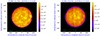 |
Fig. 1. Solar disk image at 18.3 GHz (left) and 25.8 GHz (right) obtained with the Grueff Radio Telescope on June 13, 2019, processed with the SUNDARA package (Marongiu et al. 2021). The colour bars indicate TB of the solar maps in units of Kelvin. The green circles in the lower left corner of each map mark the HPBW at the observed frequencies. |
In 2018 to mid-2023, our observations of the Sun in K band were mostly obtained at Medicina. About ∼5% of the total number of sessions were provided by the larger SRT. In the frequency range 18.1 − 26.1 GHz, we obtained an extensive data set of 327 maps. In this data set, 145 maps were obtained at 18.3 GHz, and 128 maps were obtained at 25.8 GHz. However, due to high atmospheric opacity and occasional instrumental failures, some maps (∼10%) had to be discarded, which reduced the final number to 287 maps. From 2019 to 2021, the need for a manual solar setup for each observation has limited the use of SRT in the frequency range of 18.3 − 25.5 GHz to a few solar sessions per year. This configuration resulted in 19 solar maps. Ten of these maps were observed at 18.8 GHz, and 7 were observed at 24.7 GHz. Two maps at 18.8 GHz were discarded as they were acquired under unsuitable weather conditions or were affected by instrumental failures. As shown in Fig. 2, maps with SRT were mainly performed at 18.8 and 24.7 GHz to exploit the best receiver performance and avoid radio-frequency interference (RFI).
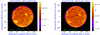 |
Fig. 2. Solar disk image at 18.8 GHz (left) and 24.7 GHz (right) obtained with SRT on January 28, 2020, processed with the SUNDARA package (Marongiu et al. 2021). See the caption of Fig. 1 for a full description of the colour bars and symbols. |
The solar maps were composed of on-the-fly (OTF) scans (Prandoni et al. 2017), commanded using the DISCOS antenna control system, in right ascension (RA, at the lower frequency) and declination (Dec, at the higher frequency). These maps cover an area of about 1.3 ° ×1.3° in the sky at Medicina (Fig. 1), and 1.5 ° ×1.5° at SRT (Fig. 2). The radio signal was processed with two different backends: (1) the full-Stokes spectropolarimeter SARDARA (theoretical bandwidth of 1.5 GHz; Melis et al. 2018) at SRT, and (2) the total-power/intensity at the Grueff Radio Telescope5, characterised by a theoretical bandwidth of 0.3 GHz. The high dynamic range of SARDARA allowed us to detect in the same image the emission from the bright solar disk and from the faint tails near the limb. The supernova remnant Cas A was selected for the absolute brightness temperature calibration (for details, see Pellizzoni et al. 2022; Mulas et al. 2022). The solar images from the Grueff Radio Telescope and SRT were extracted from the FITS files produced by the INAF solar pipeline SUNPIT (Marongiu et al. 2022). Details of the OTF mapping techniques, the setup configurations used for the receiver and backend, the observing strategy, and the data processing (RFI rejection, baseline background subtraction, and image production) are available for the Grueff Radio Telescope and SRT in the first solar paper of the SunDish Collaboration (Pellizzoni et al. 2022, and references therein). Moreover, the SunDish Archive6 includes the data set of the Grueff Radio Telescope and SRT, which is regularly updated.
3. Data analysis
We analysed and measured the size of the Sun in order to obtain information on the value of Rc, Req, and Rpol, and to study the temporal evolution of these radii. For the radius calculations we used a specific procedure that is described in Sect. 3.1. To obtain more robust measurements of the solar radii and to corroborate the presence of the coronal emission, the analysis of which will be described in detail in a further paper (Marongiu et al. 2024), we also analysed the contribution of the antenna beam pattern on the solar signal (Sect. 3.2).
3.1. Prescription for calculating the solar radius
The measurement of R⊙ at radio frequencies requires an unambiguous definition of the solar limb. This parameter is strongly influenced by the instability of the solar atmosphere. These instabilities are characterised by ever-changing small structures that are prominent in the observed radio Sun, such as active regions (ARs), sunspots, spicules, and faculae. Two widely used methods for measuring the radio R⊙ in the literature are the so-called half-power method (hereafter HP method; Costa et al. 1999; Selhorst et al. 2011, 2019a; Menezes & Valio 2017), and the inflection point of the limb-darkening function (hereafter IP method; e.g. Emilio et al. 2012, 2015; Alissandrakis et al. 2017; Menezes et al. 2021). In our analysis, both methods were applied and compared.
The HP method calculates R⊙ at the points where the brightness temperature TB is half of its quiet-Sun level (QSL) TqS (Fig. 3, top left), the most common mean temperature in the distribution of the solar disk intensity (for further details, see Landi & Chiuderi Drago 2008; Pellizzoni et al. 2022). In the IP method, the solar radius is determined by the position of the inflection-point of the solar limb-darkening profile (Fig. 3, top right); this method is less susceptible to the irregularities of the telescope beams and the variations in the TB profiles of the Sun, such as the limb-brightening level and the presence of ARs (Menezes et al. 2022).
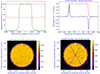 |
Fig. 3. Steps of a solar radius measurement. Top left: brightness profile with the TB levels (dashed red lines) of TqS (top line) and the half value of TqS (bottom line) used in the HP method. Top right: numerical differentiation of the brightness profile (blue curve), whose minimum and maximum points correspond to the limb coordinates of the equatorial scan (red curve) in the IP method. Bottom left: limb coordinates (white points) extracted from a solar map with a fit (circle or ellipse, solid green line). Bottom right: limb coordinates (white points) extracted from a solar map with the statistical procedure to estimate |


To determine R⊙ (with the methods described above), we followed a prescription similar to others described in the literature (Costa et al. 1999; Selhorst et al. 2019a; Menezes & Valio 2017; Menezes et al. 2021, 2022). The first step was the extraction of the solar limb coordinates from each map. These coordinates were determined considering scans, corresponding to brightness profiles (e.g. see the green curve in Fig. 3 at the top left), in both RA and Dec orientation. During the limb-point extraction, some criteria were adopted to avoid extracting limb points associated with ARs or affected by weather and seasonal effects, instrumental errors, or the high atmospheric opacity, which may increase the calculated local radius in this region and hence the average radius (Menezes & Valio 2017; Menezes et al. 2021):
-
In the HP method, we only considered coordinates within a solar ring composed of points with a centre-to-limb distance corresponding to a brightness level between 0.9 TqS and 1.1 TqS.
-
In the IP method, we only considered only scans characterised by a signal exceeding the RMS of the solar images7 (∼10 K); the limb coordinates are defined as the maximum and minimum points of the numerical derivative (blue curve in Fig. 3, top right) of each scan across the solar disk.
The second step consisted of modelling the solar limb, which is composed of the limb coordinates extracted in the first step, for each solar map. This limb was modelled following the generic parametric equation of the ellipse,
![Mathematical equation: $$ \begin{aligned} \left[\frac{X \cos {\theta } + Y \sin {\theta }}{R_{\rm eq}}\right]^2 + \left[\frac{X \sin {\theta } + Y \cos {\theta }}{R_{\rm pol}}\right]^2 = 1, \end{aligned} $$](/articles/aa/full_html/2024/04/aa48768-23/aa48768-23-eq3.gif) (1)
(1)
where θ is the ellipse orientation (set to 0 in this analysis), X = x − x0 and Y = y − y0 (x0 and y0 are the centre coordinates), and Req and Rpol indicate the semiaxes of the ellipse. Equation (1) is the case of the circle, assuming Rc = Req = Rpol. The modelling was performed using a least-squares method to determine x0, y0, and the solar radii (Rc in the circular case, and Req and Rpol in the elliptical case). The calculation of R⊙ was performed through two alternative approaches:
-
Modelling procedure: The best-fit parameters were obtained from the modelling (Eq. (1) and Fig. 3, bottom left) using either the circle or the ellipse case.
-
Statistical procedure: The radii were obtained through the median values of the centre-to-limb distances, calculated through the distance between each limb point and the fitted centre position (both in the circular and in the elliptical case). The uncertainties in the median values are described by the third and first quartiles of the sample. We calculated three average radii: (a) the average radius
 considering all the distances, (b) the equatorial radius
  only considering equatorial latitudes of the solar disk points between 30° N and 30° S, and (c) the polar radius
  only considering points above 60° N and below 60° S (Fig. 3, bottom right).
For both approaches, we filtered the final solar limb coordinates with the following iterative process:
-
The average radius
 was calculated based on the distance between each limb point and the fitted centre position. For each fit, the points with centre-to-limb distance (obtained from the modelling) between
  arcsec and
  arcsec were considered (where d = 10 arcsec for the circular fit, and d = 20 arcsec for the elliptical fit), and then a new fit was performed with the remaining points. This process was repeated until no other points were discarded.
 -
When fewer than 25 points remained, the entire map was discarded, otherwise, the radius was calculated. In the case of the statistical procedure, to calculate of Req and Rpol, we assumed a threshold of ten remaining points for each side.
-
When the standard deviation of the solar limb coordinates was smaller than 20 arcsec, then the calculated radius was stored and the next map was submitted to this process.
The same method was applied to the two INAF radio telescopes in order to compare these solar radii. The resulting radius values were further normalised at the distance of 1 AU, by correcting for the orbit eccentricity of the Earth. With this correction, the apparent R⊙ ranges between ∼950 arcsec (aphelion) and ∼1005 arcsec (perihelion) during the year.
To calculate the monthly and annual medians of our calculated R⊙, we applied a further criterion, similar to other prescriptions in the literature (e.g. Menezes et al. 2021, 2022). The following criterion reduces the scattering in the distribution of the calculated R⊙, caused by maps of low quality (affected by systematic effects of the instrument and/or bad weather conditions).
-
For each observing frequency, we calculated the average solar radius
 and only considered the values included in the range 900 − 1050 arcsec (a conservative range of R⊙ obtained through our solar observations at K band).
 -
To the remaining points (at least three), we applied the statistical Chauvenet’s criterion (Chauvenet 1863; Maples et al. 2018; Konz & Reichart 2023) to extract further outliers from our set of R⊙.
-
With the remaining points (at least three), we again calculated
 and discarded the values that were beyond the range
  arcsec.
 -
We repeated the same step for the range
 arcsec.
 -
Finally, with the remaining points (at least three), we again calculated
 and discarded the values that were beyond the more stringent
  arcsec range. This process was repeated until no other points were discarded.
The final value of R⊙ is the median of the remaining points of the sample, and the uncertainties are described by the third and first quartiles of the sample, respectively.
3.2. The role of the antenna beam pattern in the solar maps
One of the most important features that influence the measurement of R⊙ is the degrading effect of the antenna beam pattern on the solar signal (e.g. Giménez de Castro et al. 2020; Menezes et al. 2022). The analysis of this effect in our solar images allows us to (1) assess the quality of our radius determinations, and (2) reveal the presence of the coronal emission in our maps. We assess the quality of the radius determinations here. The external coronal emission observed in our solar maps and its physical nature (see the tails in the brightness profiles; green line in Fig. 3, top left) is presented in Marongiu et al. (2024). This phenomenology arises from the fact that an observed solar map results from the convolution between the beam radiation pattern of the antenna, hereafter named “beam pattern”, and the true solar signal, hereafter named “solar signal” (e.g. Wilson et al. 2013). The solar signal can be obtained from physical and/or empirical models, both using the solar maps (2D approach) and the extraction of the TB profiles as a function of the solar coordinates (1D approach). An example of these slices of the solar maps is shown in Fig. 3 (green curve, top left). To analyse the effects of the antenna beam pattern on the solar signal, we developed a specific empirical 2D model based on the convolution between the beam pattern and the solar signal. This 2D modelling procedure requires as input the observed solar map and the beam pattern (both at the same observing frequency for the given radio telescope). As output, it produces the solar signal, whose convolution with the beam pattern results in the observed solar map (the input). This output gives the empirical properties of the solar signal in terms of the size of the solar disk (Req and Rpol) and of the geometrical parameters of the external coronal emission (modelled as a 2D Gaussian function).
The Grueff and SRT beam patterns were reconstructed using GRASP, a dedicated software for the electromagnetic analysis of reflector antenna systems integrated into the TICRA tools software framework8. Excluding the measurement noise and the optical residual aberration, the measured beam patterns agree well with the GRASP nominal beam patterns (Prandoni et al. 2017; Egron et al. 2022). As shown in Figs. 4 (for Grueff) and 5 (for SRT), we used four 2D beam patterns (18.3 and 25.8 GHz for Grueff; 18.8 and 24.7 GHz for SRT). We selected these frequencies because they were employed in the vast majority of the solar maps. The single-dish nominal half-power beam width (HPBW) of Grueff and SRT at our observing frequencies ranges between 0.8 and 2.1 arcmin (Sect. 2).
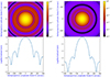 |
Fig. 4. GRASP nominal beam patterns of the Grueff Radio Telescope at 18.3 GHz (left) and at 25.8 GHz (right). Top: 2D maps of the beam pattern. Bottom: 1D equatorial TB profiles of the 2D beam pattern. All the maps are normalised in gain, and they are shown on a logarithmic scale. |
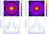 |
Fig. 5. GRASP nominal beam patterns of SRT at 18.8 GHz (left) and at 24.7 GHz (right). Top: 2D maps of the beam pattern. Bottom: 1D equatorial TB profiles of the 2D beam pattern. All the maps are normalised in gain, and they are shown on a logarithmic scale. |
The parametric model of the solar signal is defined as two normalised empirical 2D models: the ellipsis-based cylindrical box (ECB model), and the combination between the ECB model and a 2D Gaussian function (2GECB model). The ECB model, tailored only for the solar disk emission of our maps, is defined as
 (2)
(2)
where Ub is the elliptical base of the cylindrical box, defined as
![Mathematical equation: $$ \begin{aligned} U_{\rm b}(x,{ y},R_{\rm eq}, R_{\rm pol}) = \left[\frac{(x - x_{\rm C})}{R_{\rm eq}}\right]^2 + \left[\frac{({ y} - { y}_{\rm C})}{R_{\rm pol}}\right]^2, \end{aligned} $$](/articles/aa/full_html/2024/04/aa48768-23/aa48768-23-eq17.gif) (3)
(3)
where xC and yC indicate the coordinates of the ellipse centre (set to 0, as defined for the solar maps at SRT and Medicina). We used this model as a first approach to the beam pattern analysis.
The solar maps resulting from the ECB model as the solar signal convolved with the beam pattern showed that our observed solar maps display an external signal that cannot be explained simply by invoking systematic effects such as the smoothing produced by the beam pattern on the solar signal. This aspect is clearly shown in Fig. 6, where the observed limb level of the solar disk (dashed blue line) is higher than the modelled limb level obtained through the ECB model (solid red line). We will focus on this aspect in a dedicated paper (Marongiu et al. 2024). This incompatibility has led us to consider the 2GECB model, which was developed both for the solar disk and the external coronal emission (Fig. 7). This model is defined as
 (4)
(4)
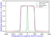 |
Fig. 6. Example of the analysis with the ECB model using the solar signal in the Grueff Radio Telescope at 18.3 GHz on September 2, 2020. The solid green line indicates the instrumental beam pattern, the dashed blue line indicates the observed equatorial TB profile of the solar map, the dotted violet line indicates the modelled equatorial TB profile of the ECB model (Eq. (3)), and the solid red line indicates the convolved best-fit TB profile using the instrumental beam pattern and the ECB model as the solar signal. |
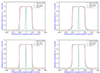 |
Fig. 7. Result of the analysis with the 2D convolution model in the context of the equatorial TB profile using the ECB model (Grueff at 18.3 GHz, top left; SRT at 18.8 GHz, bottom left) and the 2GECB model (Grueff at 18.3 GHz, top right; SRT at 18.8 GHz, bottom right). The TB profiles of the Grueff Radio Telescope were obtained on September 6, 2020; the SRT TB profiles were obtained on January 8, 2021. See the caption of Fig. 6 for a full description of the profiles. |
where Req, G and Rpol, G indicate the 1σ standard deviation among the equatorial and polar semi-axis of the 2D Gaussian function, respectively, and AG is the amplitude of the 2D Gaussian function. S indicates the sum Ub + UG, where Ub(x, y, Req, G, Rpol, G) is defined by Eq. (3), and UG indicates the ellipse-shaped 2D Gaussian function, defined as
 (5)
(5)
where H = AGe−Ub/2. This model was designed considering (1) the 2D Gaussian and the ECB model centred at xC = yC = 0, and (2) the 2D Gaussian function defined only outside the ECB model region. As we describe in Sect. 4 and discuss in Sect. 5.1, the observed solar maps are well fit with the 2D solar maps obtained through the 2D model using our beam pattern and the 2GECB model as the solar signal.
These 2D models were developed based on a Bayesian approach based on Markov chain Monte Carlo (MCMC) simulations (e.g. Sharma 2017). For this approach, we used the Python emcee package9 (Foreman-Mackey et al. 2013). The model parameters, analysed with emcee to detect degeneracies, were constrained through the definition of prior distributions (uniform in this work) that encode preliminary and general information. The complete uniform prior distribution adopted in our analysis is listed in Table 1. The parameters labelled 0 indicate the initial best-fit parameters, calculated through the maximisation of the likelihood function using the sequential least-squares programming tools available in the Python SciPy package10 (Jones et al. 2001). In the MCMC analysis, the beginning of the ensemble sampler is characterised by an initial period, called “burn in”, which is discarded by the analysis, where the convergence of the average likelihood across the chains is unstable (recommended chains: 300). The number of subsequent Markov chains was set up in 1000 steps, with a number of 20 walkers. All the uncertainties are reported at the 68% confidence level (1σ).
Uniform prior distribution adopted for the Bayesian approach in the 2D models.
4. Results
We used 304 solar maps (287 with Grueff and 17 with SRT) to calculate the radii and the correlation between the radii and the solar activity (and between Req and Rpol). We observed at seven central frequencies with Grueff and SRT: 18.1, 18.3, 18.8, 23.6, 24.7, 25.8, and 26.1 GHz. We selected four of these frequencies for our analysis. They are characterised by a uniform time coverage from 2018 to date: 18.3 and 25.8 GHz for Grueff, 18.8 and 24.7 GHz for SRT. Moreover, we also used two averaged solar maps at 18.3 and 25.8 GHz acquired in Medicina during the minimum solar activity (2018 − 2020). Our data set is composed of solar maps normalised at 1 AU, and we only considered medium- or high-quality maps to avoid undesired systematic and/or meteorological effects. These averaged maps were only obtained from the Grueff Radio Telescope because the data set obtained with SRT does not uniformly cover our temporal range of observations between 2018 and mid-2023. These results are discussed in Sect. 5. In this analysis, the images were not corrected for centre-to-limb variation (CLV) to enhance the visibility of the disk features and to simultaneously show prominences (e.g. Alissandrakis et al. 2017).
Our results from calculating the median values of Rc, Req, and Rpol are summarised in Tables 2 and 3, where the radii are listed by observing frequency, type, and method of calculation, and in Fig. 8. Following the methods described above, we obtained values of R⊙ for the various observing frequencies. These values range from 959 arcsec (obtained with the 2GECB model) to 994 arcsec (obtained with the ECB model), with typical errors of a few arcseconds.
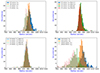 |
Fig. 8. Histograms depicting all the Req and Rpol measurements calculated from (top left) the HP- and IP methods, (top right) the statistical approach using the HP method, (bottom left) the statistical approach using the IP method, and (bottom right) the ECB and 2GECB methods. |
To check for consistency, our results of Rc are plotted in Figs. 9 (modelling approach) and 10 (statistical approach) with those from other authors at several radio frequencies and different measurement techniques (see Menezes et al. 2022, and Table 1). To guide the eye, an exponential curve (dashed line) is overplotted to show the trend of the radius as a function of the observing frequency, indicating that the radius decreases exponentially at high radio frequencies. The trend curve is just a least-squares exponential fit, not a physical model. These solar radii seem to agree within the uncertainties with the trend for the modelling and for the statistical approach (Figs. 9 and 10).
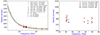 |
Fig. 9. Solar radius as a function of the observing frequency. Left: plot with our measures of Rc obtained through the modelling. The dashed lines represent the fitted exponential trend (black: all data; green: HP method; magenta: IP method). The yellow points show previous measurements from other authors (see Table 1 in Menezes & Valio 2017; Menezes et al. 2022, and references therein), and the circle and squared points are our radius values derived from Grueff and SRT. Right: plot with our measures of Rc obtained through the HP method (circle points) and the IP method (squared points). The green points indicate the measures of Rc obtained from the averaged solar maps of the Grueff Radio Telescope through the HP method (circle points) and the IP method (squared points). |
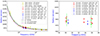 |
Fig. 10. Solar radius as a function of the observing frequency. (left) Plot with our measures of Rc obtained through the statistical approach; see the caption of Fig. 9 for a full description of the colour bars and symbols. (right) Plot with our measures of Rc obtained through the statistical approach. |
The R⊙ results (Tables 2 and 3) indicated that the HP method yields higher radius values than the IP method, as already suggested by Menezes et al. (2022) based on an analysis of the ALMA and SST data. The values derived from Grueff and SRT maps with the HP method are higher by ∼5 arcsec on average than those derived with the IP method. We note that the results of the average R⊙ measurements are comparable within an error of 1σ for the modelling and the statistical approach.
Another way to confirm these radii was to compare them with the 2D model, considering two different solar signals (ECB model and 2GECB model) and the beam patterns of the Grueff Radio Telescope and SRT (Sect. 3.2). Two examples of the application of the 2D model are shown in Fig. 7. In general, the radii obtained with the 2D convolution model using the 2GECB model are smaller by (1) 7 arcsec at least than those derived with the HP method and smaller by (2) 2 arcsec than those derived with the IP method. A specific comparison with other values obtained in the literature is described in Sect. 5.
To date, the temporal range of our data set is limited with respect to the 11-year solar activity cycle. However, we were able to investigate the temporal evolution of R⊙ and its relation with the solar activity. This activity is described through the temporal variation of the sunspot index number, collected by the SILSO data of the Royal Observatory of Belgium (Brussels)11. The strength of this relation was verified through the Pearson correlation coefficient (PCC) ρ. Applying 13-month running means to avoid the influence of annual modulations (Menezes & Valio 2017; Menezes et al. 2021) at the solar radii obtained from our maps, we obtained the values of ρ (Tables 4–6; Figs. 11 and 12). We discuss these results in Sect. 5.2. Future observations with the Grueff Radio Telescope and SRT will expand our data set, resulting in a more exhaustive analysis of this type of correlation.
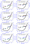 |
Fig. 11. Thirteen-month running means applied to the solar radii obtained from the Grueff maps (18.3 GHz). The red points indicate Rc, the blue points indicate Req, the green points indicate Rpol, and the black points indicate the sunspot index number. Panels a and b refer to the HP method and IP method, respectively. Panels c and d refer to the HP method and IP method, respectively, for the ellipsis-based statistical procedure. Panels e and f refer to the HP method and IP method, respectively, for the circle-based statistical procedure. Panels g and h refer to the ECB and 2GECB models, respectively. |
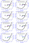 |
Fig. 12. Thirteen-month running means applied to the solar radii obtained from the Grueff maps (25.8 GHz). The red points indicate Rc, the blue points indicate Req, the green points indicate Rpol, and the black points indicate the sunspot index number. See the caption of Fig. 11 for a full description of the plots. |
Values of the correlation coefficient ρ between the solar radius (calculated with the Grueff Radio Telescope through the HP method) and the solar activity at radio frequencies characterised by a good temporal coverage.
Values of the correlation coefficient ρ between the solar radius (calculated with the Grueff Radio Telescope through the IP method) and the solar activity at radio frequencies characterised by a good temporal coverage.
Values of the correlation coefficient ρ between the solar radius (calculated with the Grueff Radio Telescope) and the solar activity at radio frequencies characterised by a good temporal coverage.
5. Discussion
5.1. Radius calculation
We obtained an accurate measure of the solar radii (Rc, Req, and Rpol) in the centimeter range (18.1 − 26.1 GHz) through single-dish observations with the Grueff Radio Telescope and SRT. Our results show a weak prolateness of the solar limb (Req > Rpol), although Req and Rpol are statistically comparable within 3σ errors (Fig. 8). This trend, as discussed by Selhorst et al. (2004), can be explained by variations in the equatorial solar atmosphere during the period of maximum activity, which causes an increase in the solar radius at lower latitudes.
We compared the calculation methods (HP, IP, statistical, ECB, and 2GECB method), and the comparison showed a variation in the calculated solar radius based on the method that was used. The values in Tables 2 and 3 show that the modelling and statistical procedures are comparable for the calculation of these mean radii within 1σ error. In general, the values of Rc obtained with the HP method in the range 18 − 26 GHz are compatible with the other radii obtained in the literature with the same method within a similar frequency range (e.g., Wrixon 1970; Fuerst et al. 1979; Costa et al. 1986; Selhorst et al. 2004, 2011). The small differences can be ascribed to the different angular resolutions of the instruments. At the same observing frequency, a lower resolution translates into values of R⊙ (and its uncertainty) that are higher than those obtained with instruments with a higher resolution. For example, the value of Rc = 976.6 ± 1.5 arcsec measured by Selhorst et al. (2004) at 17 GHz with NoRH (characterised by a spatial resolution of 10 arcsec) is (1) compatible within 1σ error with that obtained with SRT (∼979 arcsec) at 18.8 GHz, where the beam size is ∼60 arcsec, and (2) lower than that obtained with Grueff (∼982 arcsec) at 18.3 GHz, where the beam size is ∼120 arcsec, but still within 2σ error. Moreover, no significant biases arise from image measurement sampling. In our OTF technique, each pixel in the solar images is oversampled because our maps include at least six measurements per beam for each sub-scan (Pellizzoni et al. 2022). A comparison of values obtained with the IP method is not possible because no measurements in the literature are available in a frequency range comparable to ours. The available radii were calculated at observing frequencies higher than 100 GHz (e.g. Menezes et al. 2021). The mean radii obtained with the HP method and the ECB model, which are compatible with each other within 1σ error, are larger than those obtained with the IP method and the 2GECB model. This feature suggests that specific procedures for measuring R⊙ that are also designed to describe the behaviour of the solar disk (e.g. ARs) and the coronal emission (e.g. the case of the IP method and the 2GECB model), result in a lower bias in the determination of the solar radius (Menezes et al. 2022) and hence in a lower value of R⊙. In particular, the 2D solar maps modelled using our beam pattern and the 2GECB model as the solar signal (Sect. 3.2) are well fitted with the observed solar map ( ). This modelling is better than that obtained using the ECB model (
 ). Despite the statistically non-significant data set from SRT, we primarily estimate from our results (Tables 2 and 3) a possible dependence of the HP- and IP-methods on the antenna beam pattern from analysing the radius difference caused by these methods. This radius difference follows the same trend (the percentage difference ΔM between the radii obtained with the HP- and IP-method is ∼0.6%) at Grueff and SRT, suggesting that these methods could be independent of the antenna beam pattern. On the other hand, this independence is not strictly defined because at 25 GHz, this trend in the IP method seems to be less pronounced (ΔM ∼ 0.2%), suggesting a possible dependence on the antenna beam pattern. Future solar sessions at SRT will allow us to clarify this aspect. It is worth noting that approximately 30% of the R⊙ values (∼20% of Req and ∼40% of Rpol) obtained with the 2GECB model, which was built adopting a Bayesian statistics, are lower than the canonical and average optical solar photospheric radius R⊙, opt (see Fig. 8, bottom right). However, the peaks in the histogram (∼973 arcsec for Req and ∼967 arcsec for Rpol) are above R⊙, opt, and lower values are considered to be statistical fluctuations.
Figure 9 shows that our radii agree with the radius-versus-frequency trend of the literature points, where the curve seems to flatten at higher frequencies. This might explain why we obtained similar average values of the radii at our observing frequencies. In this context, it is important to take the analysis of Meftah et al. (2018) into account, who claimed an extreme weakness of the correlation between the solar radius and the observing frequency in the visible and the near-infrared, in contrast to the claim made by Rozelot et al. (2015). This weak correlation is even expected because the solar density profile near the photosphere is sharp. Meftah et al. (2018) claimed that the analysis of a possible solar radius dependence on the frequency should be based on two different regions in the solar atmosphere at least (photosphere and chromosphere). This aspect is crucial before fitting any polynomial functions to the measurements.
5.2. Time evolution of the solar radius
Despite the irregular and limited coverage in time and observing frequency of our data set, our investigation at 18.1 − 26.1 GHz of the temporal evolution of the solar radius and its relation to the solar activity suggests some interesting trends. For this correlation analysis, the SRT data set obtained at 18.8 and 24.7 GHz does not hold exhaustive information on the correlation with solar activity due to the low statistics. Therefore, we only used the data set from Grueff (at 18.3 and 25.8 GHz).
The 13-month running means applied to the solar radii measured at Medicina and the sunspot index number (Tables 4–6; Figs. 11 and 12) suggest a strong-to-moderate positive correlation between the 11-year solar activity cycle and the temporal variation in Rc and Req at all observing frequencies. Only at 25.8 GHz is a weak positive correlation obtained with the IP method. The other correlations show different results according to the approaches for the R⊙ calculation described in Sects. 3.1 and 3.2. We list the general correlation between Rpol and the solar activity below.
-
It is weakly to moderately positive at 18.3 GHz with the HP, IP, and ECB methods and at 25.8 GHz with the ECB model.
-
It is weakly negative at 25.8 GHz with the HP and IP methods.
-
It is strongly negative at 18.3 GHz and 25.8 GHz with the 2GECB model.
Finally, the correlation between Req and Rpol is listed below.
-
It is strongly positive at 18.3 GHz with the HP and IP methods.
-
It is weakly to moderately positive at 25.8 GHz with the IP method and the 2GECB model and at 18.3 GHz with the ECB model.
-
It is weakly negative at 18.3 GHz with the 2GECB model.
-
It is weakly to moderately negative at 25.8 GHz with the HP method and the ECB model.
These results suggest that specific procedures for measuring R⊙, tailored to describe both the behaviour of the solar disk and the coronal emission (e.g. the case of the IP method and the 2GECB model), show a weak-to-moderate anti-correlation between the temporal variation in Rpol and the solar activity, especially when the 2GECB model is applied. In the R⊙ prescriptions described in this work, the strength of the correlation is inversely proportional to the robustness or complexity of the prescription: for the case of the HP method, based on the TB level of the brightness profiles alone, the strength of the correlation is higher than the strengths obtained with more complex prescriptions, such as the ECB model, IP method, and the 2GECB model. In particular, the 2GECB model is also able to highlight the anti-correlation between the temporal variation of Rpol and the solar activity at 18.3 GHz, where the thermal emissions from the solar activity, a bias for the radius calculation, are generally stronger than the counterpart at 25.8 GHz.
Our results of the Medicina Grueff Radio Telescope seem to agree with the analyses presented in the literature for similar radio frequencies (Costa et al. 1999; Selhorst et al. 2004, 2011, 2019a), which are expected to be positively correlated to the solar cycle for Rc and negatively for Rpol. These results are compatible with correlations between the radius variations and the solar activity, as suggested by Menezes et al. (2021), who monitored the Sun for more than one solar cycle (from 2007 to 2019) at higher frequencies (212 and 405 GHz) with the SST and ALMA facilities. These authors suggested that the Req variations are expected to be positively correlated to the solar activity because the equatorial regions are more affected by the increase in the AR number during solar maxima, making the solar atmosphere warmer in these regions. On the other hand, Menezes et al. (2021) suggested that the anti-correlation between polar radius time series and the solar activity proxies could be explained by a possible increase in the polar limb brightening during solar minima, as also suggested by Selhorst et al. (2004).
Moreover, as shown in Fig. 11, a bump appears at 18.3 GHz at the end of 2020 in the radii and solar activity. This effect seems to corroborate a higher level of the positive correlation between R⊙ and the solar activity at this observing frequency than 25.8 GHz, which agrees with the conclusions of Menezes et al. (2021) that the solar activity in the equatorial regions is stronger at the approach of the solar maxima. Figure 12 shows that at 25.8 GHz, the time evolution of the 13-month running means applied to the measured solar radii obtained using the ECB and 2GECB models shows that this bump in the solar activity corresponds to the time when Req becomes greater than Rpol, suggesting the starting point of the rising phase of the 11-year solar activity cycle.
6. Conclusions and future developments
We mainly focus on the first measurements of the solar radius carried out using the Medicina Gavril Grueff Radio Telescope and SRT, along with a comprehensive correlation analysis that also took solar activity into account. Spanning a period of five years, from 2018 to mid-2023, we collected about 300 single-dish observations. This time frame covers approximately half of one solar cycle, and the observations were conducted in the radio K band between 18.1 GHz and 26.1 GHz. From the seven observing frequencies available during our solar sessions, we specifically chose four frequencies for our analysis. These selections were made based on their consistent time coverage. In particular, we employed frequencies of 18.3 GHz and 25.8 GHz for observations at Medicina and frequencies of 18.8 GHz and 24.7 GHz for observations at SRT. These frequencies contribute significantly to a robust and meaningful analysis of our solar radius measurements. To assess the quality of our radius determinations in our solar maps, we analysed the role of the antenna beam pattern on these maps employing two 2D models for solar emission convolved with accurate beam models, built adopting a Bayesian approach (ECB and 2GECB models).
The mean radii (Rc, Req, and Rpol) calculated in all our solar maps (for each observing frequency and radio telescope) are reported in Tables 2 and 3. They show values that are compatible with those reported in the literature. Our measurements show a weak prolateness of the solar limb (Req > Rpol), although Req and Rpol are compatible within 3σ errors. In particular, the radii calculated with the HP method and the ECB model are larger than those measured through the IP method and the 2GECB model. Moreover, while the HP method seems to be independent of the antenna beam pattern, future observations of the Sun at SRT will allow us to clarify whether the IP method is also independent of the antenna beam pattern.
As reported in Tables 4–6, the 13-month running means applied to the solar radii measured at Medicina (18.3 and 25.8 GHz) and the sunspot index number indicate (1) a positive correlation between the 11-year solar activity cycle and the temporal variation of both Rc and Req at all observing frequencies, and (2) an anti-correlation between the temporal variation of Rpol and the solar activity, especially at 25.8 GHz. Moreover, the time variation in Req and Rpol for the solar data of the Grueff Radio Telescope shows a positive correlation, especially at 18.3 GHz. Our results from the correlation analysis may indicate an agreement with the analysis presented in the literature for similar radio frequencies.
The bump observed at the end of 2020 in the radii and solar activity, especially at 18.3 GHz, constrains the positive correlation between R⊙ and the solar activity at this observing frequency. At 25.8 GHz, the time evolution of R⊙ obtained using the ECB and 2GECB models shows that the bump in the solar activity corresponds to the time when Req becomes greater than Rpol, suggesting the starting point of the rising phase of the solar activity cycle.
Our results show that specific procedures for the R⊙ measurement, suited for the modelling of the behaviour of the solar disk and the coronal emission (e.g. the case of the IP method and the 2GECB model), result in a lower bias in the solar radius determination (and hence in a lower value of R⊙) and in the detection of the anti-correlation between the temporal variation of Rpol and solar activity. This aspect suggests that the IP method, and especially the 2GECB model, could be among the most physically reliable methods for the calculation of R⊙ and its variation over time. Moreover, the radii obtained with the 2GECB model range between the values obtained with the specific theoretical atmospheric models and the HP and IP methods, suggesting that a non-negligible coronal emission level causes the decrease in the radius. We will discuss this aspect in a separate paper (Marongiu et al. 2024).
Future observations and detailed theoretical analysis with the Grueff Radio Telescope and SRT for longer periods of time and in multi-frequency approach based also on new PON receivers at SRT operating up to 116 GHz are crucial to better clarify several aspects, such as (1) the correlation between the solar activity and the solar size, (2) the polar and equatorial trends of the solar atmosphere, and (3) the question of the limb brightening (especially the polar brightening during the solar minima). This will be the subject of an upcoming work.
We did not carry out any solar observations with the Noto radio telescope because it is currently under maintenance operations.
From July 2021 this radio telescope is also equipped by the SARDARA system (Mulas et al. 2022), characterised by a theoretical bandwidth of 1.2 GHz. The scientific community can use this back-end since the observing semester 2023A.
These scans are characterised by at least a conservative 15% of the pixels with TB ≥ 0.15 TqS.
Acknowledgments
We thank the anonymous referee for helping us improve the paper. The Medicina radio telescope is funded by the Ministry of University and Research (MUR) and is operated as National Facility by the National Institute for Astrophysics (INAF). The Sardinia Radio Telescope is funded by the Ministry of University and Research (MUR), Italian Space Agency (ASI), and the Autonomous Region of Sardinia (RAS) and is operated as National Facility by the National Institute for Astrophysics (INAF). The Enhancement of the Sardinia Radio Telescope (SRT) for the study of the Universe at high radio frequencies is financially supported by the National Operative Program (Programma Operativo Nazionale – PON) of the Italian Ministry of University and Research “Research and Innovation 2014-2020”, Notice D.D. 424 of 28/02/2018 for the granting of funding aimed at strengthening research infrastructures, in implementation of the Action II.1 – Project Proposal PIR01_00010. We acknowledge the Computing Centre at INAF – Istituto di Radioastronomia for providing resources and staff support during the processing of solar data presented in this paper.
References
- Alissandrakis, C. E., Patsourakos, S., Nindos, A., & Bastian, T. S. 2017, A&A, 605, A78 [NASA ADS] [CrossRef] [EDP Sciences] [Google Scholar]
- Antia, H. M. 1998, A&A, 330, 336 [NASA ADS] [Google Scholar]
- Aschwanden, M. J. 2004, Physics of the Solar Corona. An Introduction (Berlin: Springer-Verlag) [Google Scholar]
- Auchere, F., Boulade, S., Koutchmy, S., et al. 1998, A&A, 336, L57 [NASA ADS] [Google Scholar]
- Bachurin, A. F. 1983, Izvestiya Ordena Trudovogo Krasnogo Znameni Krymskoj Astrofizicheskoj Observatorii, 68, 68 [NASA ADS] [Google Scholar]
- Belkora, L., Hurford, G. J., Gary, D. E., & Woody, D. P. 1992, ApJ, 400, 692 [Google Scholar]
- Bolli, P., Orlati, A., Stringhetti, L., et al. 2015, J. Astron. Instrum., 04, 1550008 [Google Scholar]
- Brown, R. L., Wild, W., & Cunningham, C. 2004, Adv. Space Res., 34, 555 [NASA ADS] [CrossRef] [Google Scholar]
- Bush, R. I., Emilio, M., & Kuhn, J. R. 2010, ApJ, 716, 1381 [NASA ADS] [CrossRef] [Google Scholar]
- Chapman, G. A., Dobias, J. J., & Walton, S. R. 2008, ApJ, 681, 1698 [NASA ADS] [CrossRef] [Google Scholar]
- Chauvenet, W. 1863, A Manual of Spherical and Practical Astronomy (Philadelphia: J. B. Lippincott& Co.) [Google Scholar]
- Coates, R. J. 1958, ApJ, 128, 83 [NASA ADS] [CrossRef] [Google Scholar]
- Costa, J. E. R., Homor, J. L., & Kaufmann, P. 1986, Solar Flares and Coronal Physics Using P/OF as a Research Tool, 201 [Google Scholar]
- Costa, J. E. R., Silva, A. V. R., Makhmutov, V. S., et al. 1999, ApJ, 520, L63 [NASA ADS] [CrossRef] [Google Scholar]
- Dansgaard, W., Johnsen, S. J., Reeh, N., et al. 1975, Nature, 255, 24 [CrossRef] [Google Scholar]
- Delaboudinière, J. P., Artzner, G. E., Brunaud, J., et al. 1995, Sol. Phys., 162, 291 [Google Scholar]
- Delmas, C., & Laclare, F. 2002, Sol. Phys., 209, 391 [CrossRef] [Google Scholar]
- Dziembowski, W. A., Goode, P. R., & Schou, J. 2001, ApJ, 553, 897 [NASA ADS] [CrossRef] [Google Scholar]
- Egidi, A., Caccin, B., Sofia, S., et al. 2006, Sol. Phys., 235, 407 [NASA ADS] [CrossRef] [Google Scholar]
- Egron, E., Vacca, V., Carboni, G., et al. 2022, SRT performance measurements (2018–2021), Tech. Rep. 178 [Google Scholar]
- Emilio, M., Kuhn, J. R., Bush, R. I., & Scherrer, P. 2000, ApJ, 543, 1007 [CrossRef] [Google Scholar]
- Emilio, M., Kuhn, J. R., Bush, R. I., & Scholl, I. F. 2012, ApJ, 750, 135 [NASA ADS] [CrossRef] [Google Scholar]
- Emilio, M., Couvidat, S., Bush, R. I., Kuhn, J. R., & Scholl, I. F. 2015, ApJ, 798, 48 [Google Scholar]
- Fontenla, J. M., Avrett, E. H., & Loeser, R. 1993, ApJ, 406, 319 [Google Scholar]
- Foreman-Mackey, D., Hogg, D. W., Lang, D., & Goodman, J. 2013, PASP, 125, 306 [Google Scholar]
- Fuerst, E., Hirth, W., & Lantos, P. 1979, Sol. Phys., 63, 257 [NASA ADS] [Google Scholar]
- Gilliland, R. L. 1981, ApJ, 248, 1144 [NASA ADS] [CrossRef] [Google Scholar]
- Giménez de Castro, C. G., Varela Saraiva, A. C., Costa, J. E. R., & Selhorst, C. L. 2007, A&A, 476, 369 [NASA ADS] [CrossRef] [EDP Sciences] [Google Scholar]
- Giménez de Castro, C. G., Pereira, A. L. G., Valle Silva, J. F., et al. 2020, ApJ, 902, 136 [CrossRef] [Google Scholar]
- Gleissberg, W. 1966, J. Br. Astron. Assoc., 76, 265 [NASA ADS] [Google Scholar]
- Gough, D. 2001, Nature, 410, 313 [NASA ADS] [CrossRef] [Google Scholar]
- Govoni, F., Bolli, P., Buffa, F., et al. 2021, XXXIVth General Assembly and Scientific Symposium of the International Union of Radio Science (URSI GASS), 1 [Google Scholar]
- Haberreiter, M., Schmutz, W., & Kosovichev, A. G. 2008, ApJ, 675, L53 [NASA ADS] [CrossRef] [Google Scholar]
- Hiremath, K. M., & Mandi, P. I. 2004, New Astron., 9, 651 [CrossRef] [Google Scholar]
- Hiremath, K. M., Manjunath, H., & Soon, W. 2015, New Astron., 35, 8 [NASA ADS] [CrossRef] [Google Scholar]
- Horne, K., Hurford, G. J., Zirin, H., & de Graauw, T. 1981, ApJ, 244, 340 [NASA ADS] [CrossRef] [Google Scholar]
- Jones, E., Oliphant, T., Peterson, P., et al. 2001, SciPy: Open Source Scientific Tools for Python, http://www.scipy.org [Google Scholar]
- Kaufmann, P., Parada, N. J., Magun, A., et al. 1994, Proceedings of Kofu Symposium, Kofu, Japan, 323 [Google Scholar]
- Kilic, H., & Golbasi, O. 2011, Ap&SS, 334, 75 [NASA ADS] [CrossRef] [Google Scholar]
- Konz, N., & Reichart, D. E. 2023, arXiv e-prints [arXiv:2301.07838] [Google Scholar]
- Kosovichev, A., & Rozelot, J.-P. 2018, ApJ, 861, 90 [NASA ADS] [CrossRef] [Google Scholar]
- Kosugi, T., Ishiguro, M., & Shibasaki, K. 1986, PASJ, 38, 1 [Google Scholar]
- Kuhn, J. R., Bush, R. I., Emilio, M., & Scherrer, P. H. 2004, ApJ, 613, 1241 [NASA ADS] [CrossRef] [Google Scholar]
- Laclare, F., Delmas, C., Coin, J. P., & Irbah, A. 1996, Sol. Phys., 166, 211 [NASA ADS] [CrossRef] [Google Scholar]
- Landi Degl’Innocenti, E. 2007, Fisica Solare (Milano: Springer) [Google Scholar]
- Landi, E., & Chiuderi Drago, F. 2008, ApJ, 675, 1629 [NASA ADS] [CrossRef] [Google Scholar]
- Lindsey, C., Hildebrand, R. H., Keene, J., & Whitcomb, S. E. 1981, ApJ, 248, 830 [NASA ADS] [CrossRef] [Google Scholar]
- Mamajek, E. E., Prsa, A., Torres, G., et al. 2015, arXiv e-prints [arXiv:1510.07674] [Google Scholar]
- Maples, M. P., Reichart, D. E., Konz, N. C., et al. 2018, ApJS, 238, 2 [NASA ADS] [CrossRef] [Google Scholar]
- Marongiu, M., Pellizzoni, A. P., Mulas, S., & Murtas, G. 2021, A Python Approach for Solar Data Analysis: SUNDARA (SUNDish Active Region Analyser), Preliminary Development, Tech. Rep. 81 [Google Scholar]
- Marongiu, M., Pellizzoni, A., Bachetti, M., et al. 2022, A Dedicated Pipeline to Analyse Solar Data with INAF Radio Telescopes: SUNPIT (SUNdish PIpeline Tool), Tech. Rep. 137 [Google Scholar]
- Marongiu, M.,, Pellizzoni, A., Righini, S., et al. 2024, A&A, 684, A123 (Paper II) [NASA ADS] [CrossRef] [EDP Sciences] [Google Scholar]
- Meftah, M., Corbard, T., Irbah, A., et al. 2014, A&A, 569, A60 [NASA ADS] [CrossRef] [EDP Sciences] [Google Scholar]
- Meftah, M., Corbard, T., Hauchecorne, A., et al. 2018, A&A, 616, A64 [NASA ADS] [CrossRef] [EDP Sciences] [Google Scholar]
- Melis, A., Concu, R., Trois, A., et al. 2018, J. Astron. Instrum., 7, 1850004 [NASA ADS] [CrossRef] [Google Scholar]
- Melnik, V. N., Shepelev, V. A., Poedts, S., et al. 2018, Sol. Phys., 293, 97 [CrossRef] [Google Scholar]
- Menezes, F., & Valio, A. 2017, Sol. Phys., 292, 195 [Google Scholar]
- Menezes, F., Selhorst, C. L., Giménez de Castro, C. G., & Valio, A. 2021, ApJ, 910, 77 [NASA ADS] [CrossRef] [Google Scholar]
- Menezes, F., Selhorst, C. L., Giménez de Castro, C. G., & Valio, A. 2022, MNRAS, 511, 877 [NASA ADS] [CrossRef] [Google Scholar]
- Mercier, C., & Chambe, G. 2015, A&A, 583, A101 [NASA ADS] [CrossRef] [EDP Sciences] [Google Scholar]
- Mulas, S., Pellizzoni, A., Iacolina, N. M., et al. 2022, A New Method for Accurate Calibration of Solar Disk Emission in the Radio Band, Tech. Rep. [Google Scholar]
- Nakajima, H., Nishio, M., Enome, S., et al. 1994, IEEE Proc., 82, 705 [NASA ADS] [CrossRef] [Google Scholar]
- Nakajima, H., Nishio, M., Enome, S., et al. 1995, J. Astrophys. Astron. Suppl., 16, 437 [NASA ADS] [Google Scholar]
- Neckel, H. 1995, Sol. Phys., 156, 7 [NASA ADS] [CrossRef] [Google Scholar]
- Nindos, A., Kundu, M. R., White, S. M., et al. 1999, ApJ, 527, 415 [NASA ADS] [CrossRef] [Google Scholar]
- Noël, F. 2004, A&A, 413, 725 [NASA ADS] [CrossRef] [EDP Sciences] [Google Scholar]
- Pellizzoni, A., Righini, S., Murtas, G., et al. 2019, Nuovo Cimento C Geophys. Space Phys. C, 42, 9 [Google Scholar]
- Pellizzoni, A., Righini, S., Iacolina, M. N., et al. 2022, Sol. Phys., 297, 86 [NASA ADS] [CrossRef] [Google Scholar]
- Pelyushenko, S. A., & Chernyshev, V. I. 1983, Sov. Astron., 27, 340 [NASA ADS] [Google Scholar]
- Plainaki, C., Antonucci, M., Bemporad, A., et al. 2020, J. Space Weather Space Clim., 10, 6 [NASA ADS] [CrossRef] [EDP Sciences] [Google Scholar]
- Prandoni, I., Murgia, M., Tarchi, A., et al. 2017, A&A, 608, A40 [NASA ADS] [CrossRef] [EDP Sciences] [Google Scholar]
- Prša, A., Harmanec, P., Torres, G., et al. 2016, AJ, 152, 41 [Google Scholar]
- Qu, Z. N., & Xie, J. L. 2013, ApJ, 762, 23 [NASA ADS] [CrossRef] [Google Scholar]
- Quaglia, L., Irwin, J., Emmanouilidis, K., & Pessi, A. 2021, ApJS, 256, 36 [NASA ADS] [CrossRef] [Google Scholar]
- Ramesh, R., Nataraj, H. S., Kathiravan, C., & Sastry, C. V. 2006, ApJ, 648, 707 [NASA ADS] [CrossRef] [Google Scholar]
- Reis Neto, E., Andrei, A. H., Penna, J. L., Jilinski, E. G., & Puliaev, S. P. 2003, Sol. Phys., 212, 7 [NASA ADS] [CrossRef] [Google Scholar]
- Ribes, E., Ribes, J. C., & Barthalot, R. 1987, Nature, 326, 52 [NASA ADS] [CrossRef] [Google Scholar]
- Ribes, E., Merlin, P., Ribes, J. C., & Barthalot, R. 1989, Ann. Geophys., 7, 321 [Google Scholar]
- Ribes, E., Beardsley, B., Brown, T. M., et al. 1991, in The Sun in Time, eds. C. P. Sonett, M. S. Giampapa, & M. S. Matthews, 59 [Google Scholar]
- Rozelot, J. P. 1998, Sol. Phys., 177, 321 [NASA ADS] [CrossRef] [Google Scholar]
- Rozelot, J. P., Kosovichev, A., & Kilcik, A. 2015, ApJ, 812, 91 [NASA ADS] [CrossRef] [Google Scholar]
- Rozelot, J. P., Kosovichev, A. G., & Kilcik, A. 2018, in Variability of the Sun and Sun-Like Stars: From Asteroseismology to Space Weather, eds. J. P. Rozelot, & E. S. Babayev, 89 [Google Scholar]
- Secchi, P. A. 1872, MNRAS, 32, 226 [CrossRef] [Google Scholar]
- Selhorst, C. L., Silva, A. V. R., Costa, J. E. R., & Shibasaki, K. 2003, A&A, 401, 1143 [NASA ADS] [CrossRef] [EDP Sciences] [Google Scholar]
- Selhorst, C. L., Silva, A. V. R., & Costa, J. E. R. 2004, A&A, 420, 1117 [NASA ADS] [CrossRef] [EDP Sciences] [Google Scholar]
- Selhorst, C. L., Silva, A. V. R., & Costa, J. E. R. 2005, A&A, 433, 365 [NASA ADS] [CrossRef] [EDP Sciences] [Google Scholar]
- Selhorst, C. L., Giménez de Castro, C. G., Válio, A., Costa, J. E. R., & Shibasaki, K. 2011, ApJ, 734, 64 [NASA ADS] [CrossRef] [Google Scholar]
- Selhorst, C. L., Kallunki, J., Giménez de Castro, C. G., Valio, A., & Costa, J. E. R. 2019a, Sol. Phys., 294, 175 [CrossRef] [Google Scholar]
- Selhorst, C. L., Simões, P. J. A., Brajša, R., et al. 2019b, ApJ, 871, 45 [NASA ADS] [CrossRef] [Google Scholar]
- Sharma, S. 2017, ARA&A, 55, 213 [Google Scholar]
- Shibasaki, K. 1998, in Synoptic Solar Physics, eds. K. S. Balasubramaniam, J. Harvey, & D. Rabin, ASP Conf. Ser., 140, 373 [NASA ADS] [Google Scholar]
- Simon, M., & Zirin, H. 1969, Sol. Phys., 9, 317 [NASA ADS] [CrossRef] [Google Scholar]
- Sofia, S., Dunham, D. W., Dunham, J. B., & Fiala, A. D. 1983, Nature, 304, 522 [CrossRef] [Google Scholar]
- Stuiver, M. 1980, Nature, 286, 868 [CrossRef] [Google Scholar]
- Swanson, P. N. 1973, Sol. Phys., 32, 77 [NASA ADS] [CrossRef] [Google Scholar]
- Ulrich, R. K., & Bertello, L. 1995, Nature, 377, 214 [NASA ADS] [CrossRef] [Google Scholar]
- van Haarlem, M. P., Wise, M. W., Gunst, A. W., et al. 2013, A&A, 556, A2 [NASA ADS] [CrossRef] [EDP Sciences] [Google Scholar]
- Vaquero, J. M., Svalgaard, L., Carrasco, V. M. S., et al. 2016, Sol. Phys., 291, 3061 [NASA ADS] [CrossRef] [Google Scholar]
- Vernazza, J. E., Avrett, E. H., & Loeser, R. 1981, ApJS, 45, 635 [Google Scholar]
- Wilson, T. L., Rohlfs, K., & Hüttemeister, S. 2013, Tools of Radio Astronomy (Berlin: Springer-Verlag) [Google Scholar]
- Withbroe, G. L. 1970, Sol. Phys., 11, 42 [NASA ADS] [CrossRef] [Google Scholar]
- Wittmann, A. D., Alge, E., & Bianda, M. 1993, Sol. Phys., 145, 205 [NASA ADS] [CrossRef] [Google Scholar]
- Wrixon, G. T. 1970, Nature, 227, 1231 [NASA ADS] [CrossRef] [Google Scholar]
- Zhang, P., Zucca, P., Kozarev, K., et al. 2022, ApJ, 932, 17 [CrossRef] [Google Scholar]
All Tables
Values of the correlation coefficient ρ between the solar radius (calculated with the Grueff Radio Telescope through the HP method) and the solar activity at radio frequencies characterised by a good temporal coverage.
Values of the correlation coefficient ρ between the solar radius (calculated with the Grueff Radio Telescope through the IP method) and the solar activity at radio frequencies characterised by a good temporal coverage.
Values of the correlation coefficient ρ between the solar radius (calculated with the Grueff Radio Telescope) and the solar activity at radio frequencies characterised by a good temporal coverage.
All Figures
|
Fig. 1. Solar disk image at 18.3 GHz (left) and 25.8 GHz (right) obtained with the Grueff Radio Telescope on June 13, 2019, processed with the SUNDARA package (Marongiu et al. 2021). The colour bars indicate TB of the solar maps in units of Kelvin. The green circles in the lower left corner of each map mark the HPBW at the observed frequencies. |
| In the text | |
|
Fig. 2. Solar disk image at 18.8 GHz (left) and 24.7 GHz (right) obtained with SRT on January 28, 2020, processed with the SUNDARA package (Marongiu et al. 2021). See the caption of Fig. 1 for a full description of the colour bars and symbols. |
| In the text | |
|
Fig. 3. Steps of a solar radius measurement. Top left: brightness profile with the TB levels (dashed red lines) of TqS (top line) and the half value of TqS (bottom line) used in the HP method. Top right: numerical differentiation of the brightness profile (blue curve), whose minimum and maximum points correspond to the limb coordinates of the equatorial scan (red curve) in the IP method. Bottom left: limb coordinates (white points) extracted from a solar map with a fit (circle or ellipse, solid green line). Bottom right: limb coordinates (white points) extracted from a solar map with the statistical procedure to estimate |
| In the text | |
|
Fig. 4. GRASP nominal beam patterns of the Grueff Radio Telescope at 18.3 GHz (left) and at 25.8 GHz (right). Top: 2D maps of the beam pattern. Bottom: 1D equatorial TB profiles of the 2D beam pattern. All the maps are normalised in gain, and they are shown on a logarithmic scale. |
| In the text | |
|
Fig. 5. GRASP nominal beam patterns of SRT at 18.8 GHz (left) and at 24.7 GHz (right). Top: 2D maps of the beam pattern. Bottom: 1D equatorial TB profiles of the 2D beam pattern. All the maps are normalised in gain, and they are shown on a logarithmic scale. |
| In the text | |
|
Fig. 6. Example of the analysis with the ECB model using the solar signal in the Grueff Radio Telescope at 18.3 GHz on September 2, 2020. The solid green line indicates the instrumental beam pattern, the dashed blue line indicates the observed equatorial TB profile of the solar map, the dotted violet line indicates the modelled equatorial TB profile of the ECB model (Eq. (3)), and the solid red line indicates the convolved best-fit TB profile using the instrumental beam pattern and the ECB model as the solar signal. |
| In the text | |
|
Fig. 7. Result of the analysis with the 2D convolution model in the context of the equatorial TB profile using the ECB model (Grueff at 18.3 GHz, top left; SRT at 18.8 GHz, bottom left) and the 2GECB model (Grueff at 18.3 GHz, top right; SRT at 18.8 GHz, bottom right). The TB profiles of the Grueff Radio Telescope were obtained on September 6, 2020; the SRT TB profiles were obtained on January 8, 2021. See the caption of Fig. 6 for a full description of the profiles. |
| In the text | |
|
Fig. 8. Histograms depicting all the Req and Rpol measurements calculated from (top left) the HP- and IP methods, (top right) the statistical approach using the HP method, (bottom left) the statistical approach using the IP method, and (bottom right) the ECB and 2GECB methods. |
| In the text | |
|
Fig. 9. Solar radius as a function of the observing frequency. Left: plot with our measures of Rc obtained through the modelling. The dashed lines represent the fitted exponential trend (black: all data; green: HP method; magenta: IP method). The yellow points show previous measurements from other authors (see Table 1 in Menezes & Valio 2017; Menezes et al. 2022, and references therein), and the circle and squared points are our radius values derived from Grueff and SRT. Right: plot with our measures of Rc obtained through the HP method (circle points) and the IP method (squared points). The green points indicate the measures of Rc obtained from the averaged solar maps of the Grueff Radio Telescope through the HP method (circle points) and the IP method (squared points). |
| In the text | |
|
Fig. 10. Solar radius as a function of the observing frequency. (left) Plot with our measures of Rc obtained through the statistical approach; see the caption of Fig. 9 for a full description of the colour bars and symbols. (right) Plot with our measures of Rc obtained through the statistical approach. |
| In the text | |
|
Fig. 11. Thirteen-month running means applied to the solar radii obtained from the Grueff maps (18.3 GHz). The red points indicate Rc, the blue points indicate Req, the green points indicate Rpol, and the black points indicate the sunspot index number. Panels a and b refer to the HP method and IP method, respectively. Panels c and d refer to the HP method and IP method, respectively, for the ellipsis-based statistical procedure. Panels e and f refer to the HP method and IP method, respectively, for the circle-based statistical procedure. Panels g and h refer to the ECB and 2GECB models, respectively. |
| In the text | |
|
Fig. 12. Thirteen-month running means applied to the solar radii obtained from the Grueff maps (25.8 GHz). The red points indicate Rc, the blue points indicate Req, the green points indicate Rpol, and the black points indicate the sunspot index number. See the caption of Fig. 11 for a full description of the plots. |
| In the text | |
Current usage metrics show cumulative count of Article Views (full-text article views including HTML views, PDF and ePub downloads, according to the available data) and Abstracts Views on Vision4Press platform.
Data correspond to usage on the plateform after 2015. The current usage metrics is available 48-96 hours after online publication and is updated daily on week days.
Initial download of the metrics may take a while.