| Issue |
A&A
Volume 684, April 2024
|
|
|---|---|---|
| Article Number | A161 | |
| Number of page(s) | 10 | |
| Section | Astronomical instrumentation | |
| DOI | https://doi.org/10.1051/0004-6361/202348525 | |
| Published online | 19 April 2024 | |
Optimisation-based alignment of wide-band integrated superconducting spectrometers for submillimeter astronomy
1
Faculty of Electrical Engineering, Mathematics and Computer Science, Delft University of Technology,
Mekelweg 4,
2628 CD
Delft,
The Netherlands
e-mail: This email address is being protected from spambots. You need JavaScript enabled to view it.
2
SRON-Netherlands Institute for Space Research,
Niels Bohrweg 4,
2333 CA
Leiden,
The Netherlands
3
SRON-Netherlands Institute for Space Research,
Landleven 12,
9747 AD
Groningen,
The Netherlands
4
DEMO: Electronic and Mechanical Support Division, Delft University of Technology,
Mekelweg 4,
2628 CD
Delft,
The Netherlands
5
Kitami Institute of Technology,
165 Koen-cho, Kitami,
090-8507
Hokkaido,
Japan
6
Leiden Observatory, Leiden University,
PO Box 9513,
2300 RA
Leiden,
The Netherlands
7
Faculty of Aerospace Engineering, Delft University of Technology,
Kluyverweg 1,
2629 HS
Delft,
The Netherlands
Received:
9
November
2023
Accepted:
8
February
2024
Abstract
Context. Integrated superconducting spectrometers (ISSs) for wide-band submillimeter (submm) astronomy use quasi-optical systems for coupling radiation from the telescope to the instrument. Misalignment in these systems is detrimental to the system performance. The common method of using an optical laser to align the quasi-optical components requires an accurate alignment of the laser to the submm beam from the instrument, which is not always guaranteed to a sufficient accuracy.
Aims. We develop an alignment strategy for wide-band ISSs that directly uses the submm beam of the wide-band ISS. The strategy should be applicable in both telescope and laboratory environments. Moreover, the strategy should deliver similar quality of the alignment across the spectral range of the wide-band ISS.
Methods. We measured the misalignment in a quasi-optical system operating at submm wavelengths using a novel phase and amplitude measurement scheme that is capable of simultaneously measuring the complex beam patterns of a direct-detecting ISS across a harmonic range of frequencies. The direct detection nature of the microwave kinetic inductance detectors in our device-under-test, DESHIMA 2.0, necessitates the use of this measurement scheme. Using geometrical optics, the measured misalignment, a mechanical hexapod, and an optimisation algorithm, we followed a numerical approach to optimise the positioning of corrective optics with respect to a given cost function. Laboratory measurements of the complex beam patterns were taken across a harmonic range between 205 and 391 GHz and were simulated through a model of the ASTE telescope in order to assess the performance of the optimisation at the ASTE telescope.
Results. Laboratory measurements show that the optimised optical setup corrects for tilts and offsets of the submm beam. Moreover, we find that the simulated telescope aperture efficiency is increased across the frequency range of the ISS after the optimisation.
Key words: instrumentation: spectrographs / methods: numerical
© The Authors 2024
 Open Access article, published by EDP Sciences, under the terms of the Creative Commons Attribution License (https://creativecommons.org/licenses/by/4.0), which permits unrestricted use, distribution, and reproduction in any medium, provided the original work is properly cited.
This article is published in open access under the Subscribe to Open model. This email address is being protected from spambots. You need JavaScript enabled to view it. to support open access publication.
1 Introduction
Wide-band submillimeter (submm) spectroscopy could serve as a powerful tool for studying a wide range of astrophysical phenomena (Stacey 2011). For single-pixel spectroscopy, one such target is the redshifted [CII] emission line, which can be used to probe star formation over cosmic time (Lagache et al. 2018), study the Universe at the epoch of reionisation (Gong et al. 2011), and study high-redshift dusty star-forming galaxies (Rybak et al. 2022). Multi-pixel spectrometers, also called integral field units (IFUs), can spectroscopically observe wide fields of view. This allows for studies on larger spatial scales, such as line-intensity mapping of the [CII] line (Yue et al. 2015; Yue & Ferrara 2019; Karoumpis et al. 2022), which can be used to study the growth of large-scale structure (LSS) in the early Universe. Moreover, the extragalactic rotational emission lines of CO can be used in cross-correlation power spectrum studies with other LSS tracers such as the cosmic infrared background (Maniyar et al. 2023) and the Ly-α forest signal (Qezlou et al. 2023).
Modern integrated superconducting spectrometers (ISSs) for ground-based wide-band submm astronomy, such as Super-spec (Karkare et al. 2020), μ-Spec (Mirzaei et al. 2020), and the Deep Spectroscopic High-redshift Mapper (DESHIMA; Endo et al. 2019a), rely on superconducting detectors called microwave kinetic inductance detectors (MKIDs; Day et al. 2003; Baselmans 2012) to detect incoming radiation. Unlike quasi-optical spectrometers such as CONCERTO1 (Ade et al. 2020), an ISS integrates both the detectors and the dispersive element on a single chip. This includes everything from the antenna capturing the incoming radiation and the filterbank or dispersive element that separates spectral channels to the MKID detectors. An obvious advantage of the ISS is the scalability from a single-pixel instrument to a multi-pixel IFU: because the entire device is already fabricated on a single chip, it is possible to fabricate many of these devices on a single wafer.
Coupling the broad-band single-mode signal from the telescope to the single-pixel ISS requires a good alignment of all intermediate optical components. A simple and effective design that is often adopted for heterodyne receivers (see e.g. the Atacama Large Millimeter Array (ALMA) band 5, 8, and 9 receivers; Belitsky et al. 2018; Satou et al. 2008; Baryshev et al. 2015) is to rigidly mount the wave guide feed horn of the superconductor-insulator-superconductor (SIS) mixer (Tucker & Feldman 1985) (and optionally, a simple 4 K fore-optics for polarisation separation) near the Cassegrain focus of the telescope that only relies on the movement of the secondary mirror to adjust the focus. The requirements on the cartridges and beam pointings are strict to ensure tight mechanical tolerances. However, placing the detectors in the vicinity of the telescope focus is not always possible, in which case, intermediate mirrors are introduced. For example, switching mirrors might be introduced for multiple instruments to share the same focus. Especially for instruments with direct-detection detectors that operate at sub-Kelvin temperatures, the cold detector mount tends to be more complex mechanically, and there can be a set of cold re-imaging optics to reject stray light and out-of-band thermal influx (Lamb 2003; Holland et al. 2013; Endo et al. 2019b). Each of these optical components have a finite alignment tolerance and make it hard to achieve good total optical coupling by adjusting the secondary mirror of the telescope alone. Additionally, errors in the mounting of the cryostat housing the ISS introduce alignment issues that further exascerbate the problem.
One approach to correct for the misalignment in the quasi-optical chain is to make one or more mirrors adjustable in their position. However, finding the optimum position of these components in a systematic and reproducible manner is not a trivial problem in practice. A common method is to use a visible-light laser (Catalano et al. 2022; Endo et al. 2019a), but this requires the propagation axis of the submm beam to be well aligned with the laser ray, which is not always guaranteed. Moreover, the method does not offer a way to verify the quality of the alignment in the telescope, nor does it give focal shifts.
We demonstrate a method for adjusting the position of an optical component to correct for misalignment in a submm quasi-optical system, which uses a pair of reflectors mounted on a motorised hexapod, a novel phase-and-amplitude beam-pattern measurement technique, and an optimisation algorithm. We apply the alignment method to the DESHIMA 2.0 (Taniguchi et al. 2022) submm ISS. DESHIMA 2.0 uses a wide-band leaky-lens antenna (Neto 2010; Neto et al. 2010; Hähnle et al. 2020), in combination with a superconducting filterbank (Laguna et al. 2021; Thoen et al. 2022) coupled to an array of NbTiN-hybrid MKIDs (Janssen et al. 2013), to observe the electromagnetic spectrum between 220 and 440 GHz. The MKIDs are read out using a frequency-division multiplexed readout (van Rantwijk et al. 2016), which allows for the simultaneous readout of all spectral channels. The DESHIMA 1.0 instrument saw first light (Endo et al. 2019b) at the Atacama Submillimeter Telescope Experiment (ASTE; Ezawa et al. 2004) telescope, where a 4° residual beam tilt after the laser alignment was established as a cause for the low aperture efficiency and distorted far-field beam patterns during the observations. This makes its successor, DESHIMA 2.0, a prime candidate for the development of the alignment strategy.
The paper is structured as follows: in Sect. 2.1 we start by briefly introducing the optical chain of DESHIMA 2.0: the cryo-stat optics, the cabin optics, and the ASTE Cassegrain reflector. In Sect. 2.2, we discuss the measurement technique we employed to simultaneously obtain phase-amplitude beam patterns of the ISS across a harmonic range of signal frequencies. In Sect. 2.3, we discuss that this measurement technique can be used to extract the beam misalignment with respect to the designed optical axes of the system. In Sect. 2.4, we discuss the optimisation strategy and apply this numerical approach to the alignment of a real-world optical system. In Sect. 2.5, we describe the experimental setup for the alignment procedure. In Sect. 3.1, we present results from laboratory measurements to illustrate the performance of the optimised optical setup. In Sect. 3.2, we simulate the complex beam patterns obtained from the measurements through the ASTE telescope to assess the performance and efficiencies of the aligned ISS at the telescope. Lastly, in Sect. 3.3, we qualitatively investigate the far-field patterns of the instrument.
2 Methods
2.1 Optical chain
We begin by discussing the elements in the optical path of DESHIMA 2.0 at ASTE (for a graphical overview of the optical setup, see e.g. Fig. 5.2 of Dabironezare 2020). We recreate the setup in Fig. 1 for completeness. We took the coordinate system given in Fig. 1 as our standard: Whenever we refer to an x, y, or z coordinate in this work, we refer to this system.
The first optical element encountered by radiation from the sky is the Cassegrain setup at ASTE. The primary reflector M1 is a parabolic reflector that forms a Cassegrain setup together with M2, a hyperbolic secondary reflector. The Cassegrain setup directs the light through the upper cabin, where the Cassegrain focus is located, into the lower cabin. The lower cabin houses a dual reflector, which is based on a Dragonian (Dragone 1978) reflector design. The dual reflector acts as a coupler between the Cassegrain setup and the cryostat housing of DESHIMA 2.0 and can conveniently act as correcting optics when attached to the mechanical hexapod. The dual reflector and hexapod are attached to the lower cabin ceiling by a support structure. The first dual reflector mirror in the chain, M3, is an off-axis ellipsoid. The second mirror, M4, is an off-axis hyperboloid and couples light from M3 into the cryostat. Because this dual reflector is situated outside the cryostat, it is referred to as the ‘warm optics’.
One focus of the warm optics coincides with the Cassegrain focus. This focus is located above the warm optics (see Fig. 1a) and is called the ‘warm focus’ (pWF). The plane parallel to the xy-plane containing pWF is called the ‘warm focal plane’. The second warm optics focus is located to the left of the warm optics. This focus, called the ‘cold focus’ (pCF), is located inside the cryostat and coincides with the first focus of the cryostat optics. Our coordinate system was placed such that the origin lies in pCF. The plane parallel to the yz plane and containing pCF is denoted the ‘cold focal plane’. The cryostat optics consists of a parabolic relay (Dabironezare 2020) with two off-axis paraboloid reflectors, M5 and M6, in a configuration that compensates for aberration (Murphy 1987). The cryostat optics couple the radiation entering the cryostat to the ISS, which is located below the cryostat optics in the second focus. The lower cabin ceiling acts as a mechanical reference for the placement of the entire optical setup inside the lower cabin. Therefore, any mounting errors of the cryostat and hexapod support structures amount to a misalignment of the system with respect to the entire telescope.
The final element in the optical chain is the leaky-lens antenna mounted on the DESHIMA 2.0 chip. This structure converts the radiation impinging on the lens into guided radiation that is fed to the filter bank through a co-planar wave guide.
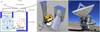 |
Fig. 1 Several figures to illustrate the optical path of DESHIMA 2.0 at ASTE. (a) Sketch of the cryostat optics, warm optics, and ASTE Cassegrain setup. In addition to the optical elements, the hexapod, cryostat, support structures, and ASTE lower and upper cabin are also sketched. The warm focal plane is denoted ‘WFP’ and the warm optics ‘WO’ in this sketch. The drawing is not to scale. The Cartesian coordinate basis is illustrated in between the cryostat and warm optics. This is the standard coordinate system for the rest of this work, (b) Render of the lower cabin setup at ASTE. The warm optics are illustrated in orange. The cryostat and hexapod support structures are attached to the lower cabin ceiling at the blue surfaces. For reference, we again show the coordinate system from a), (c) Photograph of the ASTE telescope in the Atacama desert. The primary reflector M1 and secondary reflector M2 are indicated. The lower cabin is located underneath the primary mirror in between the mounting fork. |
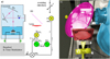 |
Fig. 2 Overview of the HPA measurement setup in front of the cryostat window, (a) Sketch of the cryostat and HPA measurement setup. In green, we plot the two signal generators SG1 and SG2. The harmonic mixers are depicted in yellow. The beam splitter, shown in pink and denoted BS, is situated such that its faces are illuminated by both mx1 and mx2. A lens, depicted in red, is placed in between mx2 and the beam splitter to increase the coupling. The modulated signal Um then travels through the cryostat to the ISS. (b) Photograph of the HPA measurement setup in front of the cryostat window. The components are colour-coded in the same fashion as in panel a. The mixer mx1 is located inside the yellow disk on the left. The material in which mx1 is embedded is a sheet of radiation-absorbing material. This prevents standing waves from generating in between mx1 and the cryostat window. In this photograph, the x-axis depicted in Fig. 1a points out of the cryostat window into the beam splitter and scanning plane. The scanning plane is oriented along the z- and y-axes. The diagonal horn containing mx2 is also shown in yellow and is visible at the bottom of the image, below the lens, which is shown in red. |
2.2 Harmonic phase-amplitude measurements
In order to assess the performance of the optimisation strategy, we need a method to calculate how our measured beam patterns would propagate through the telescope in which the device will be mounted. Coherent propagation of electromagnetic fields, taking into account diffraction from the telescope reflectors, is only possible when both the phase and amplitude (PA) patterns of the instrument are known. In addition, misalignment of the submm beam can be extracted from the PA patterns. We therefore employed a quasi-heterodyne measurement technique (Davis et al. 2019; Yates et al. 2020) that allowed us to obtain PA beam patterns of direct detectors, such as MKIDs. We specifically employed an extension to the measurement technique, called the harmonic phase and amplitude (HPA) measurement. This novel measurement technique is capable of simultaneously mapping PA beam patterns across a harmonic range of submm frequencies (see Fig. 2 for a graphical overview and the laboratory setup for the HPA measurement).
The HPA measurement technique relies on the temporal modulation of an incoming submm radiation field U1 by another submm field U2. The field U1 is generated by feeding a synthesizer signal SG1 at a frequency ƒ0 = 9.77 GHz to a harmonic mixer mx1. We used an ultrawide-band superlattice mixer (Paveliev et al. 2012) mounted in an open-ended wr4.3 wave guide. A wr4.3 to wr2.2 transition and wr2.2 corrugated horn was used as a cross check at higher frequencies to work as a single-mode source (as wr4.3 allows higher-order modes above ~260 GHz), but no difference was seen in the measured results, except for the higher signal-to-noise ratio (S/N), as the efficiency of higher harmonics increased. The mixer mx1 generates overtones at integer multiples of ƒ0 and radiates the field through the wave guide into free space, resembling a point source in its far field (Yaghjian 1984). The mixer mx1 can move in a plane, the scanning plane, which allowed us to map the instrument beam pattern as a function of the mx1 position.
The field U2 is generated by another harmonic mixer mx2, which is identical to mx1, but is fed by another synthesizer SG2 at a frequency ƒ0 + Δƒ. The mixer mx2 is fixed spatially and radiates a beam with a low opening angle into free space through a diagonal horn antenna. SG1 and SG2 generate their signals on a common clock, phase-locking U1 and U2 together. We chose Δƒ = 12.11 Hz < ƒr, where ƒr = 1.2 kHz is the sampling frequency of the MKIDs of the spectrometer. Then U1(t) = Σn An sin(2πnƒ0t + ϕn,1), with n ∈ {21,…, 41} ⊂ ℕ in our setup. This corresponds to a frequency range between 205.07 and 390.62 GHz. The mixer mx2 radiates U2(t) = Σn Bn sin(2πn(ƒ0 + Δƒ)t + ϕn,2) These two fields radiate into free space and illuminate a mylar beamsplitter, where they are added together to generate Um = U1 + U2, the modulated field. In order to increase the coupling of U2 to the MKIDs, we placed a lens between mx2 and the beam splitter. Because Um is amplitude-modulated at integer multiples of Δƒ and ƒ0, the detected power Pdet ∝ |Um|2 in the instrument is modulated at multiple modulation frequencies, with each modulation frequency corresponding to a different harmonic contained in U1,
 (1)
(1)
Here, ϕn = ϕn,1 + ϕn,2, the phase of the modulation frequency nΔƒ of Pdet· We dropped all modulation terms with a frequency higher than ƒr because these terms do not contribute to the measurable time dependence of Pdet, but contribute to the constant power entering the MKΓD. The amplitude AnBn for each modulation frequency nΔƒ can be extracted by taking the Fourier transform of Pdet(t) for each point in the scanning plane and determining the amplitudes that correspond to each nΔƒ. An example of this is illustrated in Fig. 3, where we show the raw time-stream data and Fourier transforms for three different MKIDs with filters at nf0, each simultaneously recorded at a single point in the scanning plane.
We used a phase-reference signal to extract ϕn,1 from ϕn. This signal was generated from SG1 and SG2 by feeding both signals into a subtractive mixer mxs. The resulting signal, after low-pass filtering, had a frequency Δƒ and some phase ϕref. We electronically modulated the entire instrument readout with the phase reference signal. In addition to tones coupled to MKIDs, the readout contains several ‘blind tones’ that are not coupled to any MKIDs in order to monitor temporal drift in the readout during observations. In post-processing, we can extract the phase-reference signal, and hence ϕref, by taking the Fourier transform of the blind-tone readout time-streams and identifying the amplitude and phase of the Fourier transform at Δƒ for each point in the scanning plane. After the extraction, we can use the same blind tones to remove the readout modulation from the MKID-coupled tones, which modulate at a different frequency, to further suppress any leakage of the phase reference. By referencing the phases ϕn of Pdet to the phase-reference signal phase ϕref at each source position in the scanning plane, we can spatially map the PA beam patterns across the harmonic range indexed by n.
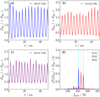 |
Fig. 3 Demonstration of the temporal modulation of Pdet as recorded during an HPA measurement. All Pdet were measured with the scanning plane centred on the beam from the ISS. (a) Raw time-stream data for Pdet of MKID 171 at 205.07 GHz. We normalised to the time-averaged power < Pdet > entering the MKID. We plot the data for a time range of 50 ms. The modulation at n∆f is visible as the rapid oscillation of the time-stream data, which has a period of about 3.9 ms. (b) Raw time-stream of MKID 96 at 214.84 GHz. (c) Raw time-stream of MKID 47 at 224.61 GHz. (d) Magnitude of the Fourier transforms of the signals in panels a, b, and c. The abscissa represents the frequencies present in the time-modulation of Pdet and is denoted by ƒmod. The dashed vertical cyan line represents the n∆f for nf0 = 205.07 GHz. Given the value of ƒ0, this corresponds to n = 21 and thus n∆f = 254.31 Hz, which is where we would expect the peak. The dashed pink line corresponds to n = 22 for nf0 = 214.84 GHz, and the dashed violet line shows n = 23, nf0 = 224.61 GHz. |
2.3 Measuring misalignment
We call a beam, defined on some plane P = P(x, y, z) ⊂ ℝ3 with a beam amplitude centre at some point p ∈ P, propagating in some direction  , misaligned with respect to an axis
  if
if
 (2)
(2)
 (3)
(3)
Expression (2) corresponds to beam offsets, where the  intersection does not coincide with p. Expression (3) corresponds to the beam tilt, where the propagation direction of the beam does not coincide with the specified axis.
We measured the beam misalignment at the cryostat by performing an HPA measurement in front of the cryostat window (see Fig. 2b for the laboratory setup). The beam is misaligned with respect to the optical axis out of the cryostat window, which corresponds to the x-axis. The optical axis originates from the cold focus pCF. The propagation direction of the beam out of the cold focal plane is denoted  .
.
Before we started the measurement, we centred mx1 on the beam from the ISS by determining the position in the scanning plane at which the MKID responses were highest. Then, we started the HPA measurement, and the beam patterns were obtained, one for each frequency nƒ0· We fitted a complex-valued, astigmatic Gaussian beam to each measured beam pattern. This fit can be used to obtain  (Tong et al. 2003; Davis et al. 2016) by also including the rotation of the plane of the Gaussian as a free parameter in the fit. This is possible because the beam tilt introduces a mismatch between the amplitude and phase centres of the beam pattern in the scanning plane (Chen et al. 2000) (see Fig. 4 for an illustration of this). Additionally, the Gaussian fit produces the location of the fitted Gaussian beam focal spot with respect to the scanning plane centre, which we assumed to be equal to pCF, the cryostat focus of the actual beam.
The hexapod and warm optics setup could also contribute to the misalignment, for example, by mounting errors of the support structure. In this case, the optical axis is the z-axis, and the point we took as reference is the warm focus pWF. The beam centre in the warm focal plane is denoted PB. The beam propagation direction out of the warm focal plane is denoted by  .
.
To measure the misalignment in the warm focal plane, we repeated the HPA measurement around the warm focal plane and calculated the beam offsets in the warm focal plane using the beam offset in the scanning plane and the Gaussian fit. The beam tilts in the scanning plane are identical to those in the warm focal plane and can be used as they are (see Fig. 5a for a sketch and Fig. 5b for a photograph of this HPA setup in the laboratory).
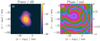 |
Fig. 4 Complex beam patterns at 205 GHz as measured with the HPA technique after the warm focal plane, with the hexapod in home configuration, (a) Amplitude pattern, (b) Phase pattern. The coordinates are with respect to the warm focus. Because they were measured in the laboratory using the setup in Fig. 5b, we used the scanning plane axes as shown in Fig. 5a, with the warm focus in the xz-plane. We denote the amplitude and phase centres with black crosses. They are different, which indicates that the beam is tilted with respect to the scanning plane normal. |
2.4 Optimisation strategy
In essence, the optimisation strategy involves simulating the warm optics and hexapod and performing ray-traces through the warm optics to calculate the optimal hexapod configuration, given some misalignment at the cryostat. All the ray-tracing calculations and simulations of the warm optics were made using the optical simulation software PyPO (Moerman et al. 2023).
We started by defining a ray representation B of a Gaussian beam (Crooker et al. 2006), oriented along the x-axis, and placing the focus in pCF. We applied the beam tilt at the cold focal plane to B by orienting B along the measured  . Then, the rays were propagated through the warm optics and into the warm focal plane, where the following cost function was evaluated:
 (4)
(4)
Here, pB represents the geometric centre of all rays in B evaluated in the warm focal plane,  is the mean propagation direction of B, phex is the simulated hexapod position, and θhex is the simulated hexapod orientation. The beam offset was optimised with respect to p0, and the beam tilt was optimised with respect to
  . In this case, p0 = pWF and
  . The parameters Δlmin and Δαmin are weights that control the required accuracy in the optimisation. In this work, we adopted the following values: Δlmin = 1 mm and Δαmin = 0.1°. We only considered the beam offset in the warm focal plane and not along the optical axis. This implies that the strategy does not explicitly correct for defocus, which is misalignment along the optical axis, but only for lateral misalignment in the warm focal plane. We find that the inclusion of the focal position in Eq. (4) by means of adding the root-mean-square (RMS) size of the ray-trace beam evaluated in the warm focal plane, divided by a weight of ΔRMSmin = 1 mm, did not produce a difference in the hexapod configuration or beam RMS size compared to an optimisation without a focal position. Including the focus with a ΔRMSmin = 0.1 mm resulted in a reduced beam RMS size, indicating that the focus was then closer to the warm focal plane, but it also resulted in a large beam offset and tilt. This indicates that at least with some misaligned initial conditions at the cold focus, it is not possible to fully correct for defocusing while at the same time having the beam intersect the warm focus at perpendicular incidence to the warm focal plane. We find that the typical distance along the z-axis between the warm focus to the ray-trace beam focus is ~100 mm, which can easily be corrected for by adjusting M2 of the ASTE telescope along the z-axis. Therefore, we did not include the focal position in Eq. (4) and optimised by only minimising the beam offset and tilt. A sketch of the local warm focal plane geometry with optimisation quantities is shown in Fig. 6.
The minimisation of Eq. (4) was performed using the differential evolution optimisation algorithm (Storn & Price 1997), which is well suited for optimisation problems with several degrees of freedom. The optimal hexapod configuration is then Popt and θopt, which are the phex and θhex corresponding to the lowest value of δ. They can be applied as a correction to the real-world hexapod to align the optical setup.
As mentioned before, the hexapod and warm optics setup could be misaligned as well, in addition to the misalignment at the cryostat window. To determine this, we first measured the beam centre  in the warm focal plane and propagation direction
  after the warm optics using the HPA method. The superscript 0 indicates that this measurement took place before the optimisation procedure. By then optimising Eq. (4) with
  , we obtained
  , the real-world translational and rotational hexapod offsets contributing to the measured beam misalignment in the warm focal plane. These hexapod offsets can then be added to the phex and θhex tried by the optimisation in Eq. (4), with p0 = pWF and
  , to take the real-world hexapod offsets into account,

The optimisation then returns the optimised hexapod translation popt and rotation θopt calculated on top of  . When applying the optimisation result to the real-world hexapod, care should be taken to only apply popt and θopt, and not
  ·
·
Then, an HPA measurement around the warm focal plane can be performed to assess the new beam centre  and propagation direction
  . Here, superscript 1 indicates that these misalignments were measured after the optimised configuration was applied to the real-world hexapod. When significant residual misalignment was present, an iterative approach was taken. To do this, we first generated a characterisation of the warm optics (see Appendix A) to determine how the hexapod degrees of freedom (DoFs) affect the beam misalignment. Using this characterisation, we selected hexapod DoFs that were to be included in the optimisation and hexapod offset finding.
The optimisation strategy can directly be applied at the telescope. This involves recreating the experimental setup shown in Fig. 5b inside the lower cabin. The mixer mx1 needs to be placed in the upper cabin (see Fig. 1a) and placed such that it faces M3.
This adaptability makes the strategy versatile because it can be applied in a variety of contexts.
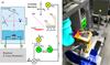 |
Fig. 5 Overview of the HPA measurement setup around the warm focal plane, (a) Sketch of the HPA measurement setup around the warm focal plane. The sketch is similar to the sketch in Fig. 2a, the only difference is the addition of the warm optics and hexapod and a change in the scanning directions resulting from the positioning of mx1. (b) Photograph of the laboratory setup, with the scanning plane after the warm optics. The laboratory setup is essentially the same as Fig. 2b, except for the addition of the warm optics, which is shown in orange. The signal generators are also visible now. The −90° rotation is around the optical axis out of the cryostat window with respect to the optical configuration shown in Fig. 2b. The laboratory photograph has the same colour-coding as the sketch in (a). Because the optical axis from the warm optics is now oriented along the y-axis, the scanning plane is now oriented along the x- and z-axes. This is also reflected in panel a. |
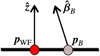 |
Fig. 6 2D sketch of the warm focal plane and the parameters described in Eq. (4). The figure is a zoom of the warm focal plane shown in Fig. 2. The misaligned-ray direction |

2.5 Experimental setup
To test the alignment procedure, we recreated the lower cabin setup at ASTE (see Fig. 5b) in the laboratory. Because the laboratory ceiling was not high enough to place mx1 above the warm optics, the warm optics and hexapod were rotated by −90° around the x-axis. This placed the warm focal plane parallel to the xz plane and the optical axis out of the warm optics parallel to the y-axis. Consequently, the beam tilts in the warm focal plane were now defined and measured with respect to the x- and z-axes instead of the x- and y-axes. Furthermore, the 30° tilt of the cryostat around the x-axis present in the ASTE lower cabin setup (see Fig. 1b) was not applied to the laboratory cryostat.
For the HPA measurements in front of the cryostat window, we placed the scanning plane about 30 cm after the cold focal plane along the positive x-axis. For the HPA measurements after the warm optics, we placed the scanning plane about 25 cm after the warm focal plane along the y-axis.
We manually measured the translation of the scanning plane from the position in front of the cryostat window to the position after the warm optics. Because we know the distance between pCF and the scanning plane centre after the cryostat window, the scanning plane translation could be used to obtain the absolute position of the scanning plane centre after the warm optics with respect to pCF, and hence pWF. This allowed us to place the measured beam centre after the warm optics in the coordinate system used for the optimisation described in Sect. 2.4 and to quantitatively assess the offset between pWF and the measured beam focus in the warm focal plane during the iterative part of the optimisation.
In order to simulate the propagation of the measured beam patterns through the Cassegrain setup at ASTE, we rotated the beam patterns back by 90° around the x-axis, so that the scanning plane normal was oriented along the z-axis. Then, we took the fitted beam focus position, averaged across the HPA frequency range, and assumed that this position overlapped the Cassegrain focus of ASTE. This allowed us to place the scanning plane in a model of ASTE and simulate the propagation of the measured beam patterns using PyPO while keeping the distance between M2 and the warm focal plane fixed at the design distance. At the real telescope, this corresponds to a focus correction by M2, as described in Sect. 2.4, such that the Cassegrain focus overlaps the fitted beam focus.
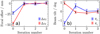 |
Fig. 7 Reduction of beam offset and tilt during the alignment procedure. (a) Decrease in focal offset, defined as pB − pWF. The red data points correspond to offsets along the z-axis, and the blue data points show offsets along the x-axis. (b) Decrease in beam tilts around the x- and z-axes. The focal offset and beam tilt are both illustrated as a function of the iteration number. Here, 0 corresponds to the setup in the hexapod home position and 1 to the initial optimised hexapod configuration. Subsequent iteration numbers correspond to steps of the iterative procedure proper. The lines are drawn between the data points to highlight the tendencies of the iterations. |
3 Results
3.1 Reduction of the beam misalignment
The first result we found was a reduction of the beam misalignment. We measured the beam tilt out of the cryostat to be  around the y- and z-axes, respectively. The misalignment around the z-axis is consistent with a rotation in the cryostat mounting, which we measured to be ∽−2.5°. We applied the iterative optimisation procedure as described. Because the hexapod DoF characterisation (see Appendix A) indicated that rotational and translational DoFs were degenerate (i.e. they have the same effect on the beam direction after the warm optics), we only included translational DoFs in the iterative optimisation.
The alignment procedure required two iterations in addition to the initial optimisation in total and took roughly 3 h. This corresponds to five HPA measurements in total, one in front of the cryostat, and four around the warm focal plane. Most of the total time was spent on the HPA measurements, which was about 30 min per measurement, 10 min of which was spent uploading and downloading measurement data. The numerical optimisation and hexapod offset finding were negligible in the time budget, each taking about 10 s to complete. This is due to the efficient multi-threaded differential evolution implementation in SciPy (Virtanen et al. 2020) and the restriction of the DoF space of the hexapod to translational DoFs. The results for the warm focal plane beam offset and beam tilt are shown in Fig. 7.
Figure 7 shows that the beam offset in the warm focal plane is already significantly reduced after the initial optimisation. The final beam offset is about 1 mm, which is smaller by an order of magnitude than the initial beam offset. The beam tilt converges more slowly, but reaches an acceptable tilt smaller than 0.1° after the second iteration.
3.2 Increase in telescope efficiency
We find that the telescope efficiency of the instrument is substantially increased by the optimisation. The measured PA beam patterns were propagated through a model of ASTE using physical optics (Balanis 1999), and the efficiency terms in Appendix B were calculated. The results are shown in Fig. 8.
The optimised setup performs considerably better than the misaligned setup in the hexapod home configuration for all three efficiencies at all measured frequencies. The secondary spillover efficiency  is slightly lower than the design value, whilst the taper efficiency ηt is slightly higher. The decrease in
  could be due to a higher illumination level at the edge of M2, which also explains the increase in ηt. Nevertheless, the aperture efficiency ηap is roughly consistent with the design value and considerably better than the misaligned values. It should be noted that for both the optimised and misaligned setup, Ruze losses (Ruze 1966) due to surface roughness of the ASTE Cassegrain were not taken into account.
We calculated the mean ηap across the frequency range for the optimised configuration to be ηap = 0.73 ± 0.04. In comparison, the home (misaligned) configuration has a mean ηap = 0.39 ± 0.03. To place this in perspective, for the optimised and home configuration, we calculated the ratio of necessary observation times to obtain the same S/N,
 (5)
(5)
where the primed quantities either denote the optimised or home configuration. Equation (5) is only valid for point sources. We find that our optimised hexapod configuration results in a decrease in the required observation time of a factor Rt = 3.5 ± 0.7. This can have a significant impact, especially for long observations that require high S/N for faint targets.
3.3 Far field analysis
We propagated the measured beam patterns to the telescope far field using PyPO and analysed the results. In Fig. 9, we show the effect of the optimisation on the half-power beam widths (HPBWs) in the E and H plane. Here, we defined the E plane to lie along the semi-minor axis of the far field main beam and the H plane to lie along the semi-major axis. We find that the HPBWs of the optimised setup are decreased with respect to the misaligned setup and are slightly smaller than the design values at all measured frequencies. This is consistent with a higher edge illumination on the secondary, which was already hypothesised as an explanation for the lower  and higher ηt. By design, the primary reflector of the telescope is under-illuminated at the edges, and by slightly increasing the illumination level towards the outer sections on the primary, we slightly decreased our beam size.
Lastly, we performed a qualitative comparison of the far-field beam patterns. We restrict the discussion to the lowest and highest measured frequencies at 205 and 391 GHz. In Fig. 10, we compare the 2D far-field beam patterns.
It is clear that the optimisation reduces the beam ellipticity. This is consistent with Eq. (4), because the optimisation criteria favour a centrally illuminated secondary. With the hexapod in home configuration, the beam pattern illuminates the secondary reflector asymmetrically. This results in an asymmetric beam pattern in the primary aperture, which gives rise to elliptical beam patterns in the far field. This also indicates that the home configuration has a lower  , as a smaller fraction of the beam pattern is intercepted by the secondary. This finding supports the observation from Fig. 8 and is another indication of the veracity of the alignment procedure.
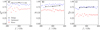 |
Fig. 8 Calculated telescope efficiencies for the ISS at ASTE. (a) Spill-over efficiency |


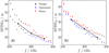 |
Fig. 9 Calculated HPBWs for the home and optimised configuration as function of signal frequency, (a) HPBWs in the E plane, (b) HPBWs in the H plane. |
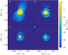 |
Fig. 10 2D far field beam patterns, (a) 205 GHz, hexapod in home configuration, (b) 205 GHz, hexapod in optimised configuration, (c) 391 GHz, hexapod in home configuration, (d) 391 GHz, hexapod in optimised configuration. All beam patterns are centred such that the beam centres are at dAz = dEl = 0 as. |
4 Conclusions
We have developed an alignment procedure for the DESHIMA 2.0 wide-band submm ISS using an optimisation strategy together with a hexapod and a modified Dragonian dual reflector. We used the novel HPA measurement technique to obtain the phase and amplitude beam patterns of the instrument and used them to quantitatively measure the misalignment in our optical chain. Because we directly used the submm beam of the ISS instead of a more conventional laser guide, we were able to accurately quantify the misalignment in the optical system. Then, using the optimisation strategy, we obtained a hexapod configuration that successfully mitigated the misalignment that was present. This was verified by laboratory measurements, which showed that the beam misalignment with the optimised hexapod configuration was sufficiently reduced. The calculated aperture efficiencies of the aligned ISS at the ASTE telescope were improved with respect to the misaligned case. Moreover, the calculated far field after the telescope showed improvement in the form of a reduced main-beam size and more symmetric beam shapes. All these findings are mutually consistent and support the veracity of the alignment procedure.
The proposed alignment procedure can be directly employed at the telescope by placing the HPA setup in the lower cabin, emulating Fig. 5b. The scanning plane itself can be placed in the ASTE upper cabin. Although this would be a complex effort due to the limited space present in the lower and upper cabin of the telescope, it is possible. For example, the scanning plane movement stage could be attached to the top of the hexaport support structure (see Fig. 1b) with the stage protruding upward into the upper cabin, allowing the scanning source itself to be located in the upper cabin and eliminating the need for additional support structures in the upper cabin. The importance of the alignment procedure can be appreciated in the context of the upcoming science verification campaign of DESHIMA 2.0. One science case of the campaign, rapid redshift surveys of dusty star-forming galaxies (Rybak et al. 2022), predicts a 400-h observation period to yield robust redshifts of the targets. This assumes a well-aligned system, and if misalignment is present, the required observation time will increase significantly.
The alignment procedure is also of interest for future extensions of the single-pixel ISS towards an ISS-based IFU. The cost function in Eq. (4) is designed to align the ISS to the optical axis of the telescope. Because the HPA technique can be used to individually measure the beam patterns of the pixels in the IFU, alignment information can be individually extracted for each pixel. Then, the optimisation procedure in this work can be used again by using a cost function that is more suitable for multi-pixel instruments.
Acknowledgements
This work was supported by the European Union (ERC Consolidator Grant No. 101043486 TIFUUN). Views and opinions expressed are however those of the authors only and do not necessarily reflect those of the European Union or the European Research Council Executive Agency. Neither the European Union nor the granting authority can be held responsible for them. T.T. was supported by the MEXT Leading Initiative for Excellent Young Researchers (Grant No. JPMXS0320200188).
Appendix A Characterising hexapod degrees of freedom
In order to link hexapod DoFs to beam misalignment parameters, a characterisation can be performed. This involves performing ray traces through the warm optics from pCF into the warm focal plane. We did not apply  to the ray-trace beam for the characterisation. For each ray-trace, we adjusted the hexapod configuration along a single DoF whilst keeping the other DoFs fixed at home position, that is, at zero translation or rotation. In this way, we characterised the effect of a single DoF on the simulated beam offset and tilt in the warm focal plane. Then, specific DoFs that are coupled to the measured beam misalignment can be selected in the matching or optimisation run. We present an example in the context of the optical system treated in this work. We show a characterisation for Z, the hexapod DoF that lies along the z-axis in Fig. 1a.
Fig. A.1 shows that this particular DoF is strongly coupled to the beam offset along the x-axis and the beam tilt around the y-axis. If a measured beam is misaligned in these two parameters, this DoF would be included in the matching-optimising steps of the iterative optimisation procedure. It is not coupled to the beam offset along the y-axis and the beam tilt around the x-axis. This indicates that if misalignment is found in any of the non-coupling parameters, another DoF needs to be considered for inclusion in the matching-optimising.
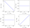 |
Fig. A.1 Beam misalignment parameters vs. the hexapod DoF along the z-axis in millimeters. The ray-trace beam is evaluated in the warm focal plane, according to Fig. 1a. a) Beam offset Δx along the x-axis in mm. b) Beam offset ∆y along the y-axis in mm. Both offsets are calculated with respect to pWF. c) Beam tilt θx around the x-axis in degrees, d) Beam tilt θy around the y-axis in degrees. |
Appendix B Telescope efficiencies
We present the expressions for  , ηt and ηap. The secondary spill-over
  was calculated over the secondary aperture and is given by
 (B.1)
(B.1)
where Ei denotes the electric field illuminating the extended reflector aperture plane  , which is defined as the spatially extended version of the secondary reflector aperture Sa. In practice, we oversized
  to have a radius three times that of Sa, so that we captured sufficient spill-over radiation. The five-point star denotes complex conjugation. This efficiency is a measure of how much illumination is intercepted by the secondary reflector. Because the spill-over losses on the primary reflector are negligible in both the misaligned and optimised configuration, they are not discussed.
The second efficiency we discuss is the taper efficiency ηt. This efficiency is a measure of the uniformity of the amplitude and phase patterns of the beam in the primary aperture plane Pa and is calculated as follows:
 (B.2)
(B.2)
where Σ denotes the physical surface area of Pa, and Ei is the electric field illuminating Pa. We always oriented the aperture in which we evaluated ηt such that the aperture normal was parallel to the telescope pointing. In this way, we calculated ηt in the direction of maximum directivity. With these two efficiencies, we can estimate the aperture efficiency ηap (Goldsmith 1998),
 (B.3)
(B.3)
Appendix C Directivities of aligned ISS
The increase in performance after aligning is also reflected in the increase in directivity of the instrument beam. The directivity depends on ηap and is given by
 (C.1)
(C.1)
Here, DdBi is the directivity in decibels (with respect to the isotropic radiator), λ is the wavelength of radiation, and Σ is the surface area of the primary aperture. Because of the prevalence of this metric in certain fields, we include the directivities in Fig. C.1 for completeness.
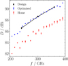 |
Fig. C.1 Directivities of the ISS after the ASTE telescope. In red, we show directivities with the hexapod in home position. In blue, we show directivities with the optimised hexapod position. In black, we show design directivities for an aligned ISS. |
References
- Ade, P., Aravena, M., Barria, E., et al. 2020, A&A, 642, A60 [NASA ADS] [CrossRef] [EDP Sciences] [Google Scholar]
- Balanis, C. A. 1999, Advanced Engineering Electromagnetics (John Wiley & Sons), 755 [Google Scholar]
- Baryshev, A. M., Hesper, R., Mena, F. P., et al. 2015, A&A, 577, A129 [NASA ADS] [CrossRef] [EDP Sciences] [Google Scholar]
- Baselmans, J. 2012, J. Low Temp. Phys., 167, 292 [CrossRef] [Google Scholar]
- Belitsky, V., Bylund, M., Desmaris, V., et al. 2018, A&A, 611, A98 [NASA ADS] [CrossRef] [EDP Sciences] [Google Scholar]
- Catalano, A., Ade, P., Aravena, M., et al. 2022, EPJ Web Conf., 257, 00010 [Google Scholar]
- Chen, M.-T., Tong, C., Papa, D., & Blundell, R. 2000, in 2000 IEEE MTT-S International Microwave Symposium Digest (Cat. No.00CH37017) (IEEE) [Google Scholar]
- Crooker, P. P., Colson, W. B., & Blau, J. 2006, Am. J. Phys., 74, 722 [NASA ADS] [CrossRef] [Google Scholar]
- Dabironezare, S. O. 2020, PhD thesis, Delft University of Technology [Google Scholar]
- Davis, K. K., Jellema, W., Yates, S. J. C., et al. 2016, IEEE Trans. Terahertz Sci. Technol., 7, 1 [CrossRef] [Google Scholar]
- Davis, K. K., Yates, S. J. C., Jellema, W., et al. 2019, IEEE Trans. Terahertz Sci. Technol., 9, 67 [Google Scholar]
- Day, P. K., LeDuc, H. G., Mazin, B. A., Vayonakis, A., & Zmuidzinas, J. 2003, Nature, 425, 817 [NASA ADS] [CrossRef] [Google Scholar]
- Dragone, C. 1978, Bell Syst. Tech. J., 57, 2663 [NASA ADS] [CrossRef] [Google Scholar]
- Endo, A., Karatsu, K., Laguna, A. P., et al. 2019a, J. Astron. Telesc. Instrum. Syst., 5, 035004 [CrossRef] [Google Scholar]
- Endo, A., Karatsu, K., Tamura, Y., et al. 2019b, Nat. Astron., 3, 989 [CrossRef] [Google Scholar]
- Ezawa, H., Kawabe, R., Kohno, K., & Yamamoto, S. 2004, in Proc. SPIE, 5489, 763 [NASA ADS] [CrossRef] [Google Scholar]
- Goldsmith, P. F. 1998, Quasioptical Systems (New York: Wiley) [CrossRef] [Google Scholar]
- Gong, Y., Cooray, A., Silva, M., et al. 2011, ApJ, 745, 49 [Google Scholar]
- Hähnle, S., Yurduseven, O., van Berkel, S., et al. 2020, IEEE Trans. Antennas Prop., 68, 5675 [CrossRef] [Google Scholar]
- Holland, W. S., Bintley, D., Chapin, E. L., et al. 2013, MNRAS, 430, 2513 [Google Scholar]
- Janssen, R. M. J., Baselmans, J. J. A., Endo, A., et al. 2013, Appl. Phys. Lett., 103, 203503 [NASA ADS] [CrossRef] [Google Scholar]
- Karkare, K. S., Barry, P. S., Bradford, C. M., et al. 2020, J. Low Temp. Phys., 199, 849 [NASA ADS] [CrossRef] [Google Scholar]
- Karoumpis, C., Magnelli, B., Romano-Díaz, E., Haslbauer, M., & Bertoldi, F. 2022, A&A, 659, A12 [NASA ADS] [CrossRef] [EDP Sciences] [Google Scholar]
- Lagache, G., Cousin, M., & Chatzikos, M. 2018, A&A, 609, A130 [NASA ADS] [CrossRef] [EDP Sciences] [Google Scholar]
- Laguna, A. P., Karatsu, K., Thoen, D., et al. 2021, IEEE Trans. Terahertz Sci. Technol., 11, 635 [Google Scholar]
- Lamb, J. 2003, IEEE Trans. Antennas Prop., 51, 2035 [CrossRef] [Google Scholar]
- Maniyar, A. S., Gkogkou, A., Coulton, W. R., et al. 2023, Phys. Rev. D, 107 [CrossRef] [Google Scholar]
- Mirzaei, M., Barrentine, E. M., Bulcha, B. T., et al. 2020, Proc. SPIE, 11453, 114530M [NASA ADS] [Google Scholar]
- Moerman, A., Gafaji, M. H., Karatsu, K., & Endo, A. 2023, J. Open Source Softw., 8, 5478 [NASA ADS] [CrossRef] [Google Scholar]
- Murphy, J. A. 1987, Int. J. Infrared Millim. Waves, 8, 1165 [Google Scholar]
- Neto, A. 2010, IEEE Trans. Antennas Prop., 58, 2238 [Google Scholar]
- Neto, A., Monni, S., & Nennie, F. 2010, IEEE Trans. Antennas Prop., 58, 2248 [CrossRef] [Google Scholar]
- Paveliev, D. G., Koshurinov, Y. I., Ivanov, A. S., et al. 2012, Semiconductors, 46, 121 [CrossRef] [Google Scholar]
- Qezlou, M., Bird, S., Lidz, A., et al. 2023, MNRAS, 524, 1933 [NASA ADS] [CrossRef] [Google Scholar]
- Ruze, J. 1966, Proc. IEEE, 54, 633 [NASA ADS] [CrossRef] [Google Scholar]
- Rybak, M., Bakx, T., Baselmans, J., et al. 2022, J. Low Temp. Phys. [Google Scholar]
- Satou, N., Sekimoto, Y., Iizuka, Y., et al. 2008, Publ. Astron. Soc. Jpn., 60, 1199 [Google Scholar]
- Stacey, G. J. 2011, IEEE Trans. Terahertz Sci. Technol., 1, 241 [CrossRef] [Google Scholar]
- Storn, R., & Price, K. 1997, J. Glob. Optim., 11, 341 [Google Scholar]
- Taniguchi, A., Bakx, T. J. L. C., Baselmans, J. J. A., et al. 2022, J. Low Temp. Phys., 209, 278 [NASA ADS] [CrossRef] [Google Scholar]
- Thoen, D. J., Murugesan, V., Laguna, A. P., et al. 2022, J. Vac. Sci. Technol. B, 40, 052603 [NASA ADS] [CrossRef] [Google Scholar]
- Tong, C.-Y., Meledin, D., Marrone, D., et al. 2003, IEEE Microw. Wirel. Compon. Lett., 13, 235 [CrossRef] [Google Scholar]
- Tucker, J. R., & Feldman, M. J. 1985, RMP, 57, 1055 [CrossRef] [Google Scholar]
- van Rantwijk, J., Grim, M., van Loon, D., et al. 2016, IEEE Trans. Microw. Theory Tech., 64, 1876 [NASA ADS] [CrossRef] [Google Scholar]
- Virtanen, P., Gommers, R., Oliphant, T. E., et al. 2020, Nature Methods, 17, 261 [CrossRef] [Google Scholar]
- Yaghjian, A. 1984, IEEE Trans. Antennas Prop., 32, 378 [CrossRef] [Google Scholar]
- Yates, S. J. C., Davis, K. K., Jellema, W., Baselmans, J. J. A., & Baryshev, A. M. 2020, J. Low Temp. Phys., 199, 156 [CrossRef] [Google Scholar]
- Yue, B., & Ferrara, A. 2019, MNRAS, 490, 1928 [NASA ADS] [CrossRef] [Google Scholar]
- Yue, B., Ferrara, A., Pallottini, A., Gallerani, S., & Vallini, L. 2015, MNRAS, 450, 3829 [NASA ADS] [CrossRef] [Google Scholar]
CarbON CII line in post-rEionisation and ReionisaTiOn epoch.
All Figures
|
Fig. 1 Several figures to illustrate the optical path of DESHIMA 2.0 at ASTE. (a) Sketch of the cryostat optics, warm optics, and ASTE Cassegrain setup. In addition to the optical elements, the hexapod, cryostat, support structures, and ASTE lower and upper cabin are also sketched. The warm focal plane is denoted ‘WFP’ and the warm optics ‘WO’ in this sketch. The drawing is not to scale. The Cartesian coordinate basis is illustrated in between the cryostat and warm optics. This is the standard coordinate system for the rest of this work, (b) Render of the lower cabin setup at ASTE. The warm optics are illustrated in orange. The cryostat and hexapod support structures are attached to the lower cabin ceiling at the blue surfaces. For reference, we again show the coordinate system from a), (c) Photograph of the ASTE telescope in the Atacama desert. The primary reflector M1 and secondary reflector M2 are indicated. The lower cabin is located underneath the primary mirror in between the mounting fork. |
| In the text | |
|
Fig. 2 Overview of the HPA measurement setup in front of the cryostat window, (a) Sketch of the cryostat and HPA measurement setup. In green, we plot the two signal generators SG1 and SG2. The harmonic mixers are depicted in yellow. The beam splitter, shown in pink and denoted BS, is situated such that its faces are illuminated by both mx1 and mx2. A lens, depicted in red, is placed in between mx2 and the beam splitter to increase the coupling. The modulated signal Um then travels through the cryostat to the ISS. (b) Photograph of the HPA measurement setup in front of the cryostat window. The components are colour-coded in the same fashion as in panel a. The mixer mx1 is located inside the yellow disk on the left. The material in which mx1 is embedded is a sheet of radiation-absorbing material. This prevents standing waves from generating in between mx1 and the cryostat window. In this photograph, the x-axis depicted in Fig. 1a points out of the cryostat window into the beam splitter and scanning plane. The scanning plane is oriented along the z- and y-axes. The diagonal horn containing mx2 is also shown in yellow and is visible at the bottom of the image, below the lens, which is shown in red. |
| In the text | |
|
Fig. 3 Demonstration of the temporal modulation of Pdet as recorded during an HPA measurement. All Pdet were measured with the scanning plane centred on the beam from the ISS. (a) Raw time-stream data for Pdet of MKID 171 at 205.07 GHz. We normalised to the time-averaged power < Pdet > entering the MKID. We plot the data for a time range of 50 ms. The modulation at n∆f is visible as the rapid oscillation of the time-stream data, which has a period of about 3.9 ms. (b) Raw time-stream of MKID 96 at 214.84 GHz. (c) Raw time-stream of MKID 47 at 224.61 GHz. (d) Magnitude of the Fourier transforms of the signals in panels a, b, and c. The abscissa represents the frequencies present in the time-modulation of Pdet and is denoted by ƒmod. The dashed vertical cyan line represents the n∆f for nf0 = 205.07 GHz. Given the value of ƒ0, this corresponds to n = 21 and thus n∆f = 254.31 Hz, which is where we would expect the peak. The dashed pink line corresponds to n = 22 for nf0 = 214.84 GHz, and the dashed violet line shows n = 23, nf0 = 224.61 GHz. |
| In the text | |
|
Fig. 4 Complex beam patterns at 205 GHz as measured with the HPA technique after the warm focal plane, with the hexapod in home configuration, (a) Amplitude pattern, (b) Phase pattern. The coordinates are with respect to the warm focus. Because they were measured in the laboratory using the setup in Fig. 5b, we used the scanning plane axes as shown in Fig. 5a, with the warm focus in the xz-plane. We denote the amplitude and phase centres with black crosses. They are different, which indicates that the beam is tilted with respect to the scanning plane normal. |
| In the text | |
|
Fig. 5 Overview of the HPA measurement setup around the warm focal plane, (a) Sketch of the HPA measurement setup around the warm focal plane. The sketch is similar to the sketch in Fig. 2a, the only difference is the addition of the warm optics and hexapod and a change in the scanning directions resulting from the positioning of mx1. (b) Photograph of the laboratory setup, with the scanning plane after the warm optics. The laboratory setup is essentially the same as Fig. 2b, except for the addition of the warm optics, which is shown in orange. The signal generators are also visible now. The −90° rotation is around the optical axis out of the cryostat window with respect to the optical configuration shown in Fig. 2b. The laboratory photograph has the same colour-coding as the sketch in (a). Because the optical axis from the warm optics is now oriented along the y-axis, the scanning plane is now oriented along the x- and z-axes. This is also reflected in panel a. |
| In the text | |
|
Fig. 6 2D sketch of the warm focal plane and the parameters described in Eq. (4). The figure is a zoom of the warm focal plane shown in Fig. 2. The misaligned-ray direction |
| In the text | |
|
Fig. 7 Reduction of beam offset and tilt during the alignment procedure. (a) Decrease in focal offset, defined as pB − pWF. The red data points correspond to offsets along the z-axis, and the blue data points show offsets along the x-axis. (b) Decrease in beam tilts around the x- and z-axes. The focal offset and beam tilt are both illustrated as a function of the iteration number. Here, 0 corresponds to the setup in the hexapod home position and 1 to the initial optimised hexapod configuration. Subsequent iteration numbers correspond to steps of the iterative procedure proper. The lines are drawn between the data points to highlight the tendencies of the iterations. |
| In the text | |
|
Fig. 8 Calculated telescope efficiencies for the ISS at ASTE. (a) Spill-over efficiency |
| In the text | |
|
Fig. 9 Calculated HPBWs for the home and optimised configuration as function of signal frequency, (a) HPBWs in the E plane, (b) HPBWs in the H plane. |
| In the text | |
|
Fig. 10 2D far field beam patterns, (a) 205 GHz, hexapod in home configuration, (b) 205 GHz, hexapod in optimised configuration, (c) 391 GHz, hexapod in home configuration, (d) 391 GHz, hexapod in optimised configuration. All beam patterns are centred such that the beam centres are at dAz = dEl = 0 as. |
| In the text | |
|
Fig. A.1 Beam misalignment parameters vs. the hexapod DoF along the z-axis in millimeters. The ray-trace beam is evaluated in the warm focal plane, according to Fig. 1a. a) Beam offset Δx along the x-axis in mm. b) Beam offset ∆y along the y-axis in mm. Both offsets are calculated with respect to pWF. c) Beam tilt θx around the x-axis in degrees, d) Beam tilt θy around the y-axis in degrees. |
| In the text | |
|
Fig. C.1 Directivities of the ISS after the ASTE telescope. In red, we show directivities with the hexapod in home position. In blue, we show directivities with the optimised hexapod position. In black, we show design directivities for an aligned ISS. |
| In the text | |
Current usage metrics show cumulative count of Article Views (full-text article views including HTML views, PDF and ePub downloads, according to the available data) and Abstracts Views on Vision4Press platform.
Data correspond to usage on the plateform after 2015. The current usage metrics is available 48-96 hours after online publication and is updated daily on week days.
Initial download of the metrics may take a while.