| Issue |
A&A
Volume 684, April 2024
|
|
|---|---|---|
| Article Number | A44 | |
| Number of page(s) | 10 | |
| Section | Numerical methods and codes | |
| DOI | https://doi.org/10.1051/0004-6361/202348073 | |
| Published online | 03 April 2024 | |
GLADEnet: A progressive web app for multi-messenger cosmology and electromagnetic follow-ups of gravitational-wave sources
1
Università degli Studi di Perugia,
06123
Perugia,
Italy
e-mail: This email address is being protected from spambots. You need JavaScript enabled to view it.
2
Istituto Nazionale di Fisica Nucleare,
Sezione di Perugia, Via A. Pascoli, 1,
06123
Perugia,
Italy
3
Universiteit Gent,
9000
Ghent,
Belgium
4
Université de Strasbourg, CNRS, Observatoire astronomique de Strasbourg, UMR 7550,
67000
Strasbourg,
France
5
INFN gruppo collegato di Parma,
Parco Area delle Scienze 7/A,
43124
Parma,
Italy
6
Università di Parma, Parco Area delle Scienze,
Parco Area delle Scienze 7/A,
43124
Parma,
Italy
7
Astronomy Research Center, Research Institute of Basic Sciences, Seoul National University,
Seoul
08826,
South Korea
8
Gran Sasso Science Institute (GSSI),
67100
L’Aquila,
Italy
9
Istituto Nazionale di Fisica Nucleare, Laboratori Nazionali del Gran Sasso,
67100
Assergi,
Italy
Received:
26
September
2023
Accepted:
9
January
2024
Abstract
Multi-messenger astronomy is an emerging field of research aimed at unravelling the physics governing astrophysical transients. GW170817 stands out as the first multi-messenger observation of the coalescence of a binary system of neutron stars, detected by the LIGO and Virgo gravitational-wave interferometers, along with space- and ground-based electromagnetic telescopes. It is a striking example of how multi-messenger observations significantly enhance our understanding of the physics of compact objects, relativistic outflows, and nucleosynthesis. It shows a new way of making cosmology and has the potential to resolve the tension between different measurements of the expansion rate of the Universe. To optimise multi-messenger observational strategies, to evaluate the efficiency of the searches for counterparts, and to identify the host galaxy of the source in a large sky localisation, information about the volumes of galaxies within the gravitational-wave localisation is of paramount importance. This requires the use of galaxy catalogues and appropriate knowledge of their completeness. Here, we describe a new interactive web tool named GLADEnet that allows us to identify catalogued galaxies and to assess the incompleteness of the catalogue of galaxies in real time across the gravitational-wave sky localisation. This measure is of particular importance when using catalogues such as the GLADE catalogue (Galaxy List for the Advanced Detector Era), which includes a collection of various catalogues that make completeness differ across different regions of the sky. We discuss the analysis steps to defining a completeness coefficient and provide a comprehensive guide on how to use the web app, detailing its functionalities. The app is geared towards managing the vast collection of over 22 million objects in GLADE. The completeness coefficient and the GLADE galaxy list will be disseminated in real time via GLADEnet, powered by the Virtual Observatory (VO) standard and tools.
Key words: gravitation / gravitational waves / catalogs / virtual observatory tools / cosmology: observations
© The Authors 2024
 Open Access article, published by EDP Sciences, under the terms of the Creative Commons Attribution License (https://creativecommons.org/licenses/by/4.0), which permits unrestricted use, distribution, and reproduction in any medium, provided the original work is properly cited.
This article is published in open access under the Subscribe to Open model. This email address is being protected from spambots. You need JavaScript enabled to view it. to support open access publication.
1 Introduction
A new era in multi-messenger astronomy began on August 17, 2017 with the momentous discovery of a gravitational-wave (GW) emission resulting from the merger of a binary system of neutron stars, GW170817 (Abbott et al. 2017a). This was accompanied by a short gamma-ray burst, GRB 170817 (Abbott et al. 2017c), followed by electromagnetic emissions across the entire electromagnetic spectrum, including an optical emission, AT2017gfo, consistent with a kilonova powered by the radioactive decay of r-process nuclei synthesised in the ejecta. Neither very high-energy gamma rays nor neutrino emissions were discovered in follow-up searches (Abbott et al. 2017b).
The One-Meter Two-Hemisphere (1M2H) Collaboration was the first to identify and announce via the Gamma-ray Coordinates Network (GCN) Circular the bright optical transient counterpart, spatially consistent with the elliptical galaxy NGC 4993, with the 1 m Swope telescope at Las Campanas Observatory in Chile (Coulter et al. 2017b). It employed an observing strategy that focused on a pre-compiled catalogue of galaxies (White et al. 2011) specifically designed to target potential host galaxies of GW sources (Coulter et al. 2017a).
The compilation of purpose-built catalogues of galaxies to be used in low-latency searches for electromagnetic counterparts of GW signals has always played a key role since the initial data acquisition of the LIGO and Virgo joint science runs (see e.g. Abadie et al. 2012; The LIGO Scientific Collaboration & Virgo Collaboration 2012; Aasi et al. 2014) up to the most recent observational campaigns (Lundquist et al. 2019; Page et al. 2020; Antier et al. 2020, Ackley et al. 2020; Paek et al. 2023, to cite a few). These catalogues include the Compact Binary Coalescence Galaxy catalogue (CBCG; Kopparapu et al. 2008), the Gravitational Wave Galaxy Catalogue (GWGC; White et al. 2011), the Galaxy List for the Advanced Detector Era (GLADE; Dálya et al. 2018), the Census of the Local Universe (CLU; Cook et al. 2019), the Heraklion Extragalactic Catalogue (HECATE; Kovlakas et al. 2021), and the NASA/IPAC Extragalactic Database (NED) Local Volume Sample, NED-LVS, (Cook et al. 2023).
One of the main challenges in the search for the EM counterpart is the large sky localisation associated with a GW signal with respect to the field of view of the electromagnetic telescopes. The use of a galaxy catalogue enables the size of the region being observed to be reduced by limiting follow-up research to the known galaxies located within the GW sky localisation (Gehrels et al. 2016; Singer et al. 2016a; Arcavi et al. 2017; Abbott et al. 2019).
This approach allows us to optimise the use of observational resources by increasing the efficiency and effectiveness of the follow-up campaigns also involving telescopes with narrow fields of view. When potential counterparts are identified, the galaxy catalogue’s information (such as position, size, distance, and the colour index) also allows observers to prioritise observations and data collection in order to characterise the most promising candidates. Over the years, a few platforms have been developed to release lists of galaxies within the localisation regions of Gw sources: the NED Gravitational Wave Follow-up (GWF) Service1 (Cook et al. 2023), Mass AssociatioN for GRavitational waves Observations Efficiency (MANGROVE2; Ducoin et al. 2020), and the Hunt Of Gravitational Wave Areas for Rapid Transients (HOGWARTs3; Salmon et al. 2020).
In multi-messenger cosmology, galaxy catalogues also hold a noteworthy role in the context of the statistical or galaxy catalogue dark siren method for statistical cosmological inference, starting from the pioneering work of Schutz (1986) and revisited in a Bayesian framework by several authors (Del Pozzo 2012; Chen et al. 2018; Nair et al. 2018; Soares-Santos et al. 2019; Fishbach et al. 2019; Gray et al. 2020). Under this approach, catalogues of galaxies are utilised to identify potential hosts within the localisation volume of a GW event.
The importance of knowing the incompleteness of catalogues is an aspect largely discussed for cross-matching and ranked galaxy strategies (Hanna et al. 2014; Singer et al. 2016b; Coughlin et al. 2018; Cook et al. 2023). It also represents a crucial aspect with significant implications in post-observation analysis, aiming to estimate the efficiency of galaxy-targeted searches. This involves evaluating the probability that observed galaxies are the actual hosts of the signal in comparison to all the galaxies within the GW volume, as is discussed, for example, in Ackley et al. (2020). The catalogues’ completeness is extremely relevant for cosmological investigations (Gray et al. 2022; Finke et al. 2021), especially in the context of dark standard sirens when catalogue-based approaches are utilised (see gwcosmo, Gray et al. 2020 and icarogw, Mastrogiovanni et al. 2023). This study aims to provide an estimate of the completeness of the GLADE catalogue within the localisation volumes of GW sources through the definition of a sky-localisation-dependent completeness parameter, which we refer to as C. As GLADE comprises various catalogues, each exhibiting different levels of completeness, this coefficient aims to provide an accurate completeness evaluation in each region of sky volume corresponding to each GW event.
The list of galaxies and the completeness coefficient will be made available through an interactive web app, GLADEnet, for the published gravitational-wave transient catalogues GWTC-2.1 and GWTC-3 (The LIGO Scientific Collaboration & Virgo Collaboration 2021; LIGO Scientific Collaboration 2023). For the low-latency candidate events, the app will listen and upload the candidates from the GCN4 in an automated way, including early-warning alerts (Magee et al. 2021).
The article is structured into the following sections. In Sect. 2, we introduce the GLADE catalogue and conduct a comprehensive analysis of its density map. In Sect. 3, we assess the intrinsic luminosity function of GLADE that was employed during the analysis. We used the last version of the GLADE releases; as of the time of writing, GLADE+ is the most up-to-date version. In Sect. 4, we define and compute the completeness coefficient, C. In Sect. 5, we explore the technology utilised in developing GLADEnet, including its graphical user interface, and present some illustrative examples of its application. Finally, in Sect. 6 we provide the findings and future directions of this work, with a focus on the prospects for third-generation ground-based interferometers such as the Einstein Telescope (ET; Punturo et al. 2010) and Cosmic Explorer (Reitze et al. 2019; Evans et al. 2023).
In the present work, we assume a flat ΛCDM cosmology with parameters from Planck Collaboration VI (2020): H0 = 100 h = 67.4 km s−1Mpc−1, ΩM = 0.31, and Ωλ = 0.68.
2 The GLADE catalogue
GLADE is a comprehensive catalogue specifically designed to aid the identification of the host galaxies of GW events and their potential transient counterparts (Dálya et al. 2018). GLADE serves an important role in facilitating electromagnetic (EM) follow-up campaigns for GW candidates, as well as providing valuable insights into the matter distribution in the local Universe and contributing to the study of the Hubble flow (Abbott et al. 2021c, 2023; Raffai et al. 2024).
The catalogue is periodically updated, and the latest version is referred to as GLADE+. The current version is formed by cross-matching six different, though not independent, astronomical catalogues: GWGC (White et al. 2011), 2MPZ (Bilicki et al. 2013), 2MASS XSC (Huchra et al. 2012), HyperLEDA (Makarov et al. 2014), WISExSCOSPZ (Bilicki et al. 2016), and SDSS-DR16Q (Lyke et al. 2020), encompassing a total of approximately 22.5 million galaxies and 750 thousand quasars (Dálya et al. 2022). This study does not consider the list of active galactic nuclei (AGN) gathered in GLADE+ and instead focuses solely on the collection of galaxies.
GLADE+ density map
Figure 1 shows the density map of GLADE+. The plot was obtained with the Aladin Sky Atlas − v12.0 (Bonnarel et al. 2000) using the functionalities in the data collection tree5. Already on visual inspection, the non-uniform galaxy density in the catalogue shows up (see e.g. the red and blue boxes on the right side of Fig. 1). The plane of the Milky Way is readily visible, as the gas and dust in the Galactic plane absorb electromagnetic radiation. Then, the anisotropies mainly stem from the diverse sensitivities of various survey campaigns conducted by different facilities.
For the Galactic extinction, which gives rise to sky regions of significant incompleteness, we compared the main regions of diminished galaxy density within the GLADE density map with the all-sky Galactic reddening map provided by Schlegel et al. (1998). This map is accessible via the Analysis Center for Extended Data (CADE)6. We employed the method described in Greco et al. (2022a), where extinction regions beyond a specific threshold are encoded using the Multi-Order Coverage (MOC) data structure (Fernique et al. 2015). This approach has been extended to encompass the credible areas associated with GW sky localisations, facilitating easy comparison among irregularly shaped sky regions and enabling queries of IVOA (International Virtual Observatory Alliance) data providers, as is demonstrated in Greco et al. (2019, 2022b).
Figure 1 displays the green MOC map of the reddening region, which corresponds to an area of 10 481 deg2 with extinction values greater than 0.2. This region will be also visualised in the GLADEnet application, and the value of a potential intersection between this map and the localisation area of a GW source will be given in the ‘GW sky area ∩ reddening map’; more details can be found within Sect. 5.
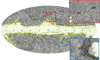 |
Fig. 1 Galaxy distribution of the GLADE+ catalogue superimposed on the MOC maps (green) derived from the reddening map by Schlegel et al. (1998), presented within the galactic frame using a Mollweide projection. The MOC contour has an extinction value >0.2 with an area = 10481 deg2. The red and blue boxes are zooms showing two examples of anisotropies in the galaxy distribution, possibly due to surveys with different sensitivities covering the region. |
3 Estimating Schechter function parameters
The Schechter function was employed to characterise the luminosity distribution of galaxies in a given sample, providing valuable insights into their population and evolution (Schechter 1976).
The Schechter function can be defined in terms of absolute magnitudes (González et al. 2006; Hill et al. 2010; Gehrels et al. 2016; Dálya et al. 2018),
 (1)
(1)
where Φ* is the normalisation factor, α* is the faint-end slope, M* is the characteristic absolute magnitude, Mi is the absolute magnitude of the ¡th galaxy, and M* is directly linked to the characteristic luminosity, with  . The completeness analysis presented in Dálya et al. (2022) demonstrates that the GLADE+ catalogue includes all of the brightest galaxies, contributing 90% of the total B-band luminosity up to a luminosity distance of dL ≃ 130 Mpc.
For our more thorough analysis, we aim is to find the best-fit Schechter function parameters for the GLADE+ catalogue and calculate its completeness using them. Our purpose is to determine the intrinsic Schechter function specific to the selected catalogue, independently of previous studies. To be more specific, we evaluated a proper set of the Schechter function parameters,  , from the GLADE+ catalogue. The new best-fit adjustment would provide an operational Schechter function profile, which would be compared to the luminosity function of the galaxies confined into the credible volume of a GW sky localisation. This was undertaken with the objective of calculating the new parameter, the completeness coefficient denoted as C, consistently for each GW localisation volume, cross-matching the galaxies compiled in the GLADE+ catalogue. Further discussion of the completeness coefficient is provided in Sect. 4.
In order to achieve this, first we discarded the region near the galactic plane with a cut of |b| > 20° in the galactic latitude. Hence, we excluded approximately three million objects whose lines of sight fall within the galactic plane (see Fig. 2). We conducted separate analyses for the northern and southern hemispheres to ascertain whether there are any notable differences in the catalogue between different galactic latitudes. No significant variation was observed between the two distributions; therefore, the luminosity function of GLADE+ will be determined by combining the data from both polar caps up to a conservative luminosity distance of 75 Mpc. At such a distance, the galaxy catalogue is complete (Dálya et al. 2022), allowing for the estimation of Schechter parameters (see Sect. 3) without having to additionally compensate for missing galaxies.
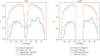 |
Fig. 2 Distribution of GLADE+ galaxies before (left) and after approximately 3 million galaxies were excluded, primarily because they are located within the galactic plane. Among the remaining galaxies, more than 17 million (in red) lack apparent K-magnitude values, while roughly 707 000 (in blue) have no apparent B-magnitude information. Lastly, there are approximately 760 000 sources (in green) with information available for both bands. |
Fitting procedure
After selecting the galaxies, as was described in the preceding section, we proceeded to fit the distribution of GLADE+ galaxies using the Schechter function.
Three distinct volume shells with radii ranging from 25 Mpc to 75 Mpc were chosen for the analysis. To initiate the fitting process, we used the Schechter parameters from Gehrels et al. (2016).
Figure 3 shows the absolute B magnitude distribution up to 75 Mpc together with our best-fit Schechter function, shown as a blue curve.
The error bands at 1σ, 3σ, and 5σ confidence levels are also represented in varying shades of light blue. For the analysis, we adopted the curve_fit7 method from the Python Scipy library (Virtanen et al. 2020). The error estimation for the counts was computed, taking into account a Poisson distribution. The sources were grouped into 30 bins, each having a width of 0.2. Ultimately, the derived values from our fitting, averaged across the three distinct shells, are presented in Table 1 and are consistent, within the error, with that reported in Gehrels et al. (2016) and Dálya et al. (2022).
Having obtained the intrinsic parameters, we are able to perform coherent completeness analyses inside a GW credible volume.
Galaxy luminosity function values from the literature and our fitting results for the GLADE+ catalogue.
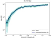 |
Fig. 3 Schechter function fitting for GLADE+ up to 75 Mpc; B-band filter. The GLADE+ galaxy distribution is shown in black with three different error bands in light blue, corresponding to 1σ, 3σ, and 5σ confidence levels. The resulting fit is shown in blue with medium parameter values of |

4 The completeness coefficient
The completeness coefficient, C, is determined as the ratio of the total luminosity of galaxies inside the credible volume of a GW sky localisation, ℒGW × GLADE+, to the total luminosity expected based on the Schechter function, ℒ = jL × VGW, where jL is the value obtained by integrating the Schechter function over the luminosity. Here, we computed the luminosity density (with integral bound x1 = 0) utilising the following equation:
 (2)
(2)
where Γ(α + 2, x1) is the incomplete gamma function.
The completeness coefficient, C, is evaluated as
 (3)
(3)
We estimate C for 86 events from the GWTC-2.1 and GWTC-3 catalogues (The LIGO Scientific Collaboration & Virgo Collaboration 2021; LIGO Scientific Collaboration 2023). These events present the mixed waveform analysis, plus the multi-messenger event, GW170817. Considering the low signal-to-noise ratio (S/N) and the unphysical dominance in the posterior, as is reported in Table IV of LIGO Scientific Collaboration (2023), we opted not to include GW200322_091133 and GW200308_173609 from the O3b run. Instead, by using the GLADEnet tool, users can explore all the events and select the waveform model according to the guidelines provided in Sect. 5.1. The results are summarised in Table A.1. Each event is presented with the 90% credible volume within which we computed the apparent magnitude threshold (mth,B) and the corresponding C coefficients. The upper panel of Fig. 4 illustrates the comparison of the completeness coefficient distributions obtained for GLADE+ and those obtained with another version of the same catalogue, GLADE v2.3 (Dálya et al. 2018), on the data server Vizier8. GLADE+ improves the estimate of the completeness coefficient by approximately one order of magnitude, shifting the tail of low values from C ~ 10−4 to C ~ 10−3. The lower panel of Fig. 4 displays the completeness coefficient for both GLADE+ and GLADE v. 2.3 as a function of the credible localisation volume. The distribution shows an approximate trend where the completeness coefficient decreases as the volume increases. In this distribution, the well-localised events GW170817 (Abbott et al. 2017b) and GW190814_211039 (Abbott et al. 2020a) are clearly evident in the top left corner with Cgw170817 ~ 3.4 and Cgw190814_211039 ~ 6.7 × 10⁻¹, respectively.
Completeness plots
For enhanced data visualisation, we generated a plot showcasing the completeness within the credible localisation volumes of a GW event. By way of example, Fig. 5 displays the completeness plot of GW190814_211039. Black dots represent the distribution of GLADE+ galaxies in the B photometric band within the 90% credible volume. The expected Schechter function, calculated in Sect. 3, is displayed as a dash-dotted green line, while the one using parameters from the literature in Gehrels et al. (2016) is represented by blue dots for comparison.
To determine the optimal histogram bin width, we employed Knuth’s rule (Knuth 2018), as it has been implemented in the astropy library9. Knuth’s rule is a Bayesian method used to determine the most suitable bin width for a histogram by considering a fixed-width approach.
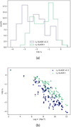 |
Fig. 4 Completeness coefficient distributions in the B band, CB, for the 86 selected events. Top panel a: histogram of CB values obtained using GLADE+ (green line) and the older version of GLADE, 2.3, (dashed histogram) on a logarithmic scale. Bottom panel b: scatter plot illustrating CB dependency on the localisation volume. Green triangles represent data from the updated galaxy catalogue, while blue circles represent data from the older one. |
5 GLADEnet: a progressive web app
GLADEnet10 is a progressive app that enables interactive visualisation and filtering of galaxies confined within the 90% credibility region of a GW sky localisation. GLADEnet is developed using ReactJS11. ReactJS is a JavaScript library used for building user interfaces in web development with a component-based approach that enables developers to create reusable user interface (UI) components.
With the second observational run of the LIGO and Virgo Collaborations, a 3D map was released for compact binary coalescence (CBC) events, which includes information about the event’s distance (Singer et al. 2016a; Abbott et al. 2019). To obtain the galaxies within the 90% credible volume, we utilised the crossmatch function provided by the ligo.skymap library12. The galaxy catalogue utilised in GLADEnet is based on the most up-to-date version of GLADE. At the time of writing, the latest version of GLADE is GLADE+.
GLADEnet uses 3D sky maps to select and visualise galaxies within the sky localisation volume and enables users to evaluate the completeness of the corresponding galaxy catalogue. Figure 6 depicts the graphical user interface of GLADEnet, which includes a drop-down menu for event selection. If the chosen event corresponds to one from the GWTCs, labelled as GW, you can further select the waveform model used in the parameter estimation (PE; see Sect. 5.1 for a detailed explanation). In the case of a candidate event sent in low latency, they are denoted as S, and the user can choose the sequence of LVK alerts sent for that specific event. The waveform banks used in the post-processing analysis are specified in the publications related to the GWTCs (The LIGO Scientific Collaboration & Virgo Collaboration 2021; LIGO Scientific Collaboration 2023). The timeline of alerts issued for the GW event candidates and the corresponding information on the source parameters released at different times with respect to the merger are fully described in the IGWN Public Alerts User Guide13, specifically in the data analysis section14.
The completeness plot is displayed within a dedicated resizable box and the coefficient, C, is reported in a contextual table.
The interactive galaxy visualisation is powered by Aladin Lite, displaying GLADE+ objects located within the 90% localisation volume (see Fig. 7). By utilising a slider, positioned below the Aladin Lite canvas, you can filter galaxies based on their absolute magnitude (B MAG) or the 3D probability density per Mpc3 (dp_dV) at the positions of each target, as is defined in Singer et al. (2016b). Applying more than one filter simultaneously is currently not allowed. We plan to add a multi-filter functionality in a future version.
The graphical visualisation is complemented by a map that shows regions with a low galaxy density in GLADE+ due to Galactic absorption. This map is overlaid with the GW sky localisation area and is constructed as described in Sect. 3.
The GLADE+ extinction map is shown in red in Fig. 7. This map can assist users in assessing whether the event is located in the direction of the Milky Way, enabling them to evaluate potential data loss due to the presence of gases and dust. This information helps in setting appropriate observational strategies, such as the use of suitable photometric filters. In addition to the graphical visualisation, we will provide the intersection percentage between the extinction map and the localisation area using the MOC approach (Greco et al. 2022a).
Considering the constraints of a web browser application, we limit the display to the first 1000 galaxies. However, the users can download the rest of the table to their local machine using the dedicated graphical functionality.
The complete source code is publicly accessible on GitHub15.
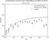 |
Fig. 5 Completeness plot for GW190814_211039. The black dots represent the distribution of the GLADE+ galaxies in the B photometric band within the 90% credible volume. The expected GLADE+ Schechter-function is displayed as a dash-dotted green line and compared with the one from Gehrels et al. (2016) shown with blue dots. |
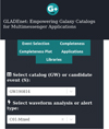 |
Fig. 6 GLADEnet user interface. The drop-down menu enables event selection. If the chosen event corresponds to one from the GWTCs, labelled as GW, the user can further select the waveform family used for the source parameter estimation. In the case of a candidate event sent with low latency, denoted as S, the user can choose the initial or updated information sent for that specific event. |
 |
Fig. 7 Interactive visualisation powered by Aladin Lite. The zoomed-in box displays in orange boxes the GLADE+ galaxies located within the 90% localisation volume (blue regions) of the GW190814 event. The plane of the Milky Way is shown with the red MOC map. |
5.1 Low latency and catalogued event modelling
As was previously described, the GLADEnet app provides both low-latency GW candidates, identified as S events, and catalogued published events. The initial low-latency sky map was obtained by Bayestar (Singer & Price 2016), whose conditional distribution of distance was obtained with the product of a Gaussian likelihood. These sky maps are followed in low latency by updated sky maps produced by Bayesian Bilby (Ashton et al. 2019; or LaLinference in the past; Veitch et al. 2015) algorithms. Over a longer timescale, the offline full Bayesian parameter estimation gives the most accurate parameter estimation, which can differ from the low-latency ones.
Analysing GW signals, different waveform models are applied. Each waveform model can infer slightly different parameter values for the source. This also causes some differences in the source localisation, namely in the 2D sky maps and in the 3D sky localisation volumes. Using the lower drop-down menu displayed in Fig. 6, the user can select the waveform model corresponding to each specific analysis. For BBH events, three different waveform models are used by the LVK Collaboration (LIGO Scientific Collaboration 2023): the IMRPhenomXPHM model, the SEOBNRv4PHM model, and the Mixed. IMRPhenomXPHM (Pratten et al. 2021) takes a phenomenological approach to extract the waveform, while SEOBNRv4PHM takes an effective one-body (EOB) approach (Ossokine et al. 2020). Finally, the Mixed model is just a weighted combination of the previous ones. For binary neutron stars (BNSs) and neutron star-black hole (NSBH) events, more waveform models are applied to account for specific effects, such as neutron star tidal effects (Abbott et al. 2021a, 2020b, 2021b).
For the catalogued events, the GLADEnet app makes available the different analysis results so that the user can choose the ones corresponding to a specific waveform model of interest or instead compare different model results. However, if the user is not interested in a specific waveform model, we suggest using the Mixed analyses, whose values are reported in the final Table A.1. On the GLADEnet page, the completeness coefficient is relative to the sky maps obtained by the offline parameter estimation and published in the catalogues (see Zenodo repository16).
5.2 Supporting GLADE catalogue versions
In the current development phase, the GLADEnet app automatically ingests the latest version of the GLADE catalogue and provides results accordingly. The utilised version of GLADE is explicitly stated in the legend of the completeness graph and prominently featured in the introductory paragraph of the application. A novel catalogue, UpGLADE, is currently in development, encompassing data across the ugriz and W1–W4 bands. The future migration to UpGLADE will assimilate recent surveys, including the Legacy Survey and Pan-STARRS (Dálya et al., in prep.). While GLADEnet will consistently generate results during the continuous updates of the GLADE release, similar to the aforementioned UpGLADE, extending it to any other galaxy catalogue will require the implementation of new functionalities planned in the forthcoming versions. It is noteworthy that, currently, local tables, FITS images, and MOC maps can be uploaded by right-clicking on the Aladin LITE canvas to test and compare tables from different collections.
5.3 Applications
The capabilities developed within GLADEnet will have several key applications. We provide a brief overview of some of them.
(i) Choice of observational strategy: GLADEnet will assist in selecting the observational strategy based on galaxy completeness and the magnitude threshold. The observational strategy depends both on the sky localisation area and on catalogue completeness. In the latter case, when completeness is low, covering the entire sky region with wide-field telescopes is needed due to the lack of many galaxies in the catalogue, while when the completeness coefficient is high, targeting galaxies with telescopes with smaller fields of view is optimal for following up on the probable host (Singer et al. 2016a). In this framework, GLADEnet can be used to promote punctual surveys and to maximise the follow-up campaigns identifying sky regions that are currently less observed or incomplete, so as to increase the catalogue completeness. Once the observation campaigns have been carried out, the new data can be uploaded directly to the VizieR data server. The VizieR upload service17 is dedicated to uploading and preparing the addition of a new catalogue. The Centre de Données astronomiques de Strasbourg (CDS) provides a full description of the standard conventions used18. The user has the freedom to define the strategy according to C. In future publications, some user-optimised target cases will be explored and suggested to the user.
(ii) Search efficiency estimates: the completeness evaluation by GLADEnet is linked to the probability that the observed galaxies are the actual hosts of the GW source, and is extrapolated directly from the Crossmatch method (Singer et al. 2016b). It is possible to see the dp_dV value, the probability density of being a host of the GW event at the positions of each target, and other properties by clicking on the possible host visualised on the Aladin window.
(iii) Support for the Hubble constant estimate: the punctual survey inside the GW event localisation could identify the most likely host galaxies based on their position and intrinsic properties, as is mentioned in the first item, and lead to a reduction in false positives (Singer et al. 2016a). The ad hoc observation could increase the number of galaxies in the catalogue, leading to an increase in catalogue completeness, a fundamental parameter in the gwcosmo catalogue method of cosmological inference (Gray et al. 2022).
6 Conclusion and future prospects
The paper presents a new interactive web tool named GLADEnet, which is able to evaluate the completeness of the GLADE+ galaxy catalogue within the sky localisation volume of GW signals.
Using GLADE+ galaxies, we built the luminosity function described by a Schechter function. The estimated best-fit Schechter function parameters are consistent with the previously published one (see e.g. Gehrels et al. 2016). We then defined the coefficient, estimating the completeness of the credible volume of a GW event by comparing the galaxies within this volume and the GLADE+ luminosity function.
Using GLADEnet, we then derived the completeness coefficient, C, for each gravitational event detected during the LVK observational runs (O1, O2, and O3). GLADEnet will be used in real time for current and future low-latency alerts. At present, new events, labelled as “S” in the application, are uploaded periodically or in response to the discovery of interesting detections that may necessitate a prompt follow-up.
We plan to add simulated events, which will be useful for defining observational strategies for upcoming runs. The application was completely developed within the framework of the Virtual Observatory in order to extend and use FAIR (findable, accessible, interoperable, and reusable) astronomical standards.
Here, we focus on the photometric B band, but this will also be extended to other bands of the electromagnetic spectrum, particularly the K band. The B and K filter bands are preferred as indicators of the BNS formation rate in various astrophysical models and BNS formation channels (see e.g. Zwart & Yungelson 1998; Belczynski et al. 2002; Rasio & Shapiro 2002; Vigna-Gómez et al. 2018; Andrews & Mandel 2019; Neijssel et al. 2019), and they are influenced differently by interstellar and Galactic dust and gases (Hill et al. 2010).
We also intend to conduct future studies to investigate red-shift dependencies, examining their potential impact on the density of galaxies within the 3D volume and on the luminosity function. Indeed, in Eq. (1), the characterisation of the absolute magnitude,  , and the normalisation factor density,
  , will be essential (Lin et al. 1999; Loveday et al. 2015; Wilson 2022). Here, Q and P represent the luminosity and density evolution parameters, respectively. This consideration becomes crucial because, going to more sensitive detectors, we expect that a large number of host galaxy candidates will be distributed across larger and larger redshifts. Accounting for redshift will be imperative for cosmological inference with third-generation detectors such as ET (Punturo et al. 2010; Maggiore et al. 2020) and Cosmic Explorer (Reitze et al. 2019), which will have the potential to investigate sources far beyond the local Universe (Ronchini et al. 2022). For instance, ET detection of BNSs extends up to z ~ 2–3, while BBH mergers could potentially be detected at redshifts as high as z ~ 5 (Maggiore et al. 2020; Branchesi et al. 2023). In this scenario, the redshift uncertainty associated with galaxies becomes a crucial factor. The impact of redshift uncertainties on the Hubble constant inference has already been explored in Turski et al. (2023). Consequently, the Schechter function’s evolution will be investigated with a focus on redshift uncertainties: many sources at the distances from which GWs from BBHs originate only have photometric redshift estimates available, which, compared to spectroscopic redshifts, are significantly less accurate.
Thinking about the future, this web tool will be extended to include the more and more complete catalogues expected from instruments such as Euclid (Euclid Collaboration 2022). The application uses GLADE+ but can be extended to the future version of GLADE, as is described in Sect. 5.2 (Gergely et al., in prep.). We are planning to include other galaxy catalogues present in Vizier that image large sky areas in different optical bands, such as the DESI Legacy Surveys (Dey et al. 2019) and Pan-STARRS (Chambers et al. 2016).
Acknowledgements
The research leading to these results has received funding from the European Union’s Horizon 2020 Programme under the AHEAD2020 project (grant agreement n. 871158). We acknowledge the INFN and ASI support under ASI-INFN agreement no. 2021-43-HH.0. Research is also supported by Italian Ministry of University and Research (MUR) through the program “Dipartimenti di Eccellenza 2023-2027” (Grant SUPER-C), Italy and by Italian Ministry of University and Research (MUR) through the program “Dipartimenti di Eccellenza 2023–2027” (Grant SUPER-C), Italy and PRIN 2020KB33TP: “Multimessenger astronomy in the Einstein Telescope Era (METE)”. E.K. is supported by the National Research Foundation of Korea 2021M3F7A1082056. The authors like to thank S. Palmerini, S. Germani, P.C. Orestano, S. Rinaldi, and C. Turski for fruitful discussions throughout the project. The authors would also like to thank T. Scocciolini for his valuable assistance in designing the GLADEnet logo. The authors are grateful to for the excellent support from the computing service at INFN Perugia provided by F. Gentile and E. Becchetti. We express our gratitude to the anonymous referee who has enabled us to enhance our work through invaluable suggestions and corrections.
Appendix A C values
C values for GW events.
References
- Aasi, J., Abadie, J., Abbott, B. P., et al. 2014, ApJS, 211, 7 [NASA ADS] [CrossRef] [Google Scholar]
- Abadie, J., Abbott, B. P., Abbott, R., et al. 2012, A&A, 541, A155 [NASA ADS] [CrossRef] [EDP Sciences] [Google Scholar]
- Abbott, B. P., Abbott, R., Abbott, T. D., et al. 2017a, Phys. Rev. Lett., 119, 161101 [Google Scholar]
- Abbott, B. P., Abbott, R., Abbott, T. D., et al. 2017b, ApJ, 848, L12 [Google Scholar]
- Abbott, B. P., Abbott, R., Abbott, T. D., et al. 2017c, ApJ, 848, L13 [CrossRef] [Google Scholar]
- Abbott, B. P., Abbott, R., Abbott, T. D., et al. 2019, ApJ, 875, 161 [NASA ADS] [CrossRef] [Google Scholar]
- Abbott, R., Abbott, T. D., Abraham, S., et al. 2020a, ApJ, 896, L44 [Google Scholar]
- Abbott, B. P., Abbott, R., Abbott, T. D., et al. 2020b, ApJ, 892, L3 [NASA ADS] [CrossRef] [Google Scholar]
- Abbott, B. P., Abbott, R., Abbott, T. D., et al. 2021a, ApJ, 909, 218 [NASA ADS] [CrossRef] [Google Scholar]
- Abbott, R., Abbott, T. D., Abraham, S., et al. 2021b, ApJ, 915, L5 [NASA ADS] [CrossRef] [Google Scholar]
- Abbott, B. P., Abbott, R., Abbott, T. D., et al. 2021c, ApJ, 909, 218 [NASA ADS] [CrossRef] [Google Scholar]
- Abbott, R., Abe, H., Acernese, F., et al. 2023, ApJ, 949, 76 [NASA ADS] [CrossRef] [Google Scholar]
- Ackley, K., Amati, L., Barbieri, C., et al. 2020, A&A, 643, A113 [NASA ADS] [CrossRef] [EDP Sciences] [Google Scholar]
- Andrews, J. J., & Mandel, I. 2019, ApJ, 880, L8 [NASA ADS] [CrossRef] [Google Scholar]
- Antier, S., Agayeva, S., Almualla, M., et al. 2020, MNRAS, 497, 5518 [NASA ADS] [CrossRef] [Google Scholar]
- Arcavi, I., McCully, C., Hosseinzadeh, G., et al. 2017, ApJ, 848, L33 [NASA ADS] [CrossRef] [Google Scholar]
- Ashton, G., Hübner, M., Lasky, P. D., et al. 2019, ApJS, 241, 27 [NASA ADS] [CrossRef] [Google Scholar]
- Belczynski, K., Kalogera, V., & Bulik, T. 2002, ApJ, 572, 407 [NASA ADS] [CrossRef] [Google Scholar]
- Bilicki, M., Jarrett, T. H., Peacock, J. A., Cluver, M. E., & Steward, L. 2013, ApJS, 210, 9 [NASA ADS] [CrossRef] [Google Scholar]
- Bilicki, M., Peacock, J. A., Jarrett, T. H., et al. 2016, ApJS, 225, 5 [Google Scholar]
- Bonnarel, F., Fernique, P., Bienaymé, O., et al. 2000, A&AS, 143, 33 [NASA ADS] [CrossRef] [EDP Sciences] [Google Scholar]
- Branchesi, M., Maggiore, M., Alonso, D., et al. 2023, J. Cosmology Astropart. Phys., 2023, 068 [CrossRef] [Google Scholar]
- Chambers, K. C., Magnier, E. A., Metcalfe, N., et al. 2016, arXiv e-prints [arXiv:1612.05560] [Google Scholar]
- Chen, H.-Y., Fishbach, M., & Holz, D. E. 2018, Nature, 562, 545 [Google Scholar]
- Cook, D. O., Kasliwal, M. M., Van Sistine, A., et al. 2019, ApJ, 880, 7 [Google Scholar]
- Cook, D. O., Mazzarella, J. M., Helou, G., et al. 2023, ApJS, 268, 14 [NASA ADS] [CrossRef] [Google Scholar]
- Coughlin, M. W., Tao, D., Chan, M. L., et al. 2018, MNRAS, 478, 692 [CrossRef] [Google Scholar]
- Coulter, D. A., Foley, R. J., Kilpatrick, C. D., et al. 2017a, Science, 358, 1556 [NASA ADS] [CrossRef] [Google Scholar]
- Coulter, D. A., Kilpatrick, C. D., Siebert, M. R., et al. 2017b, GRB Coordinates Network, 21529, 1 [NASA ADS] [Google Scholar]
- Dálya, G., Galgóczi, G., Dobos, L., et al. 2018, MNRAS, 479, 2374 [Google Scholar]
- Dálya, G., Díaz, R., Bouchet, F. R., et al. 2022, MNRAS, 514, 1403 [CrossRef] [Google Scholar]
- Del Pozzo, W. 2012, Phys. Rev. D, 86, 043011 [NASA ADS] [CrossRef] [Google Scholar]
- Dey, A., Schlegel, D. J., Lang, D., et al. 2019, AJ, 157, 168 [Google Scholar]
- Ducoin, J. G., Corre, D., Leroy, N., & Le Floch, E. 2020, MNRAS, 492, 4768 [NASA ADS] [CrossRef] [Google Scholar]
- Euclid Collaboration (Scaramella, R., et al.) 2022, A&A, 662, A112 [NASA ADS] [CrossRef] [EDP Sciences] [Google Scholar]
- Evans, M., Corsi, A., Afle, C., et al. 2023, arXiv e-prints [arXiv: 2306.13745] [Google Scholar]
- Fernique, P., Boch, T., Donaldson, T., et al. 2015, IVOA Recommendation [Google Scholar]
- Finke, A., Foffa, S., Iacovelli, F., Maggiore, M., & Mancarella, M. 2021, J. Cosmol. Astropart. Phys., 2021, 026 [CrossRef] [Google Scholar]
- Fishbach, M., Gray, R., Hernandez, I. M., et al. 2019, ApJ, 871, L13 [NASA ADS] [CrossRef] [Google Scholar]
- Gehrels, N., Cannizzo, J. K., Kanner, J., et al. 2016, ApJ, 820, 136 [CrossRef] [Google Scholar]
- González, R. E., Lares, M., Lambas, D. G., & Valotto, C. 2006, A&A, 445, 51 [NASA ADS] [CrossRef] [EDP Sciences] [Google Scholar]
- Gray, R., Hernandez, I. M., Qi, H., et al. 2020, Phys. Rev. D, 101, 122001 [NASA ADS] [CrossRef] [Google Scholar]
- Gray, R., Messenger, C., & Veitch, J. 2022, MNRAS, 512, 1127 [NASA ADS] [CrossRef] [Google Scholar]
- Greco, G., Branchesi, M., Chassande-Mottin, E., et al. 2019, PoS, Asterics2019, 031 [Google Scholar]
- Greco, G., Punturo, M., Allen, M., et al. 2022a, Astron. Comput., 39, 100547 [NASA ADS] [CrossRef] [Google Scholar]
- Greco, G., Branchesi, M., Punturo, M., et al. 2022b, in ASP Conf. Ser., 532, eds. J. E. Ruiz, F. Pierfedereci, & P. Teuben, 131 [NASA ADS] [Google Scholar]
- Hanna, C., Mandel, I., & Vousden, W. 2014, ApJ, 784, 8 [NASA ADS] [CrossRef] [Google Scholar]
- Hill, D. T., Driver, S. P., Cameron, E., et al. 2010, MNRAS, 404, 1215 [NASA ADS] [Google Scholar]
- Huchra, J. P., Macri, L. M., Masters, K. L., et al. 2012, ApJS, 199, 26 [Google Scholar]
- Knuth, K. H. 2018, Astrophysics Source Code Library, [record ascl:1803.013] [Google Scholar]
- Kopparapu, R. K., Hanna, C., Kalogera, V., et al. 2008, ApJ, 675, 1459 [NASA ADS] [CrossRef] [Google Scholar]
- Kovlakas, K., Zezas, A., Andrews, J. J., et al. 2021, MNRAS, 506, 1896 [NASA ADS] [CrossRef] [Google Scholar]
- Lin, H., Yee, H. K. C., Carlberg, R. G., et al. 1999, ApJ, 518, 533 [NASA ADS] [CrossRef] [Google Scholar]
- Loveday, J., Norberg, P., Baldry, I. K., et al. 2015, MNRAS, 451, 1540 [NASA ADS] [CrossRef] [Google Scholar]
- Lundquist, M. J., Paterson, K., Fong, W., et al. 2019, ApJ, 881, L26 [NASA ADS] [CrossRef] [Google Scholar]
- Lyke, B. W., Higley, A. N., McLane, J. N., et al. 2020, ApJS, 250, 8 [NASA ADS] [CrossRef] [Google Scholar]
- Magee, R., Chatterjee, D., Singer, L. P., et al. 2021, ApJ, 910, L21 [NASA ADS] [CrossRef] [Google Scholar]
- Maggiore, M., Broeck, C. V. D., Bartolo, N., et al. 2020, J. Cosmol. Astropart. Phys., 2020, 050 [CrossRef] [Google Scholar]
- Makarov, D., Prugniel, P., Terekhova, N., Courtois, H., & Vauglin, I. 2014, A&A, 570, A13 [NASA ADS] [CrossRef] [EDP Sciences] [Google Scholar]
- Mastrogiovanni, S., Pierra, G., Perriès, S., et al. 2023, arXiv e-prints [arXiv:2305.17973] [Google Scholar]
- Nair, R., Bose, S., & Saini, T. D. 2018, Phys. Rev. D, 98, 023502 [CrossRef] [Google Scholar]
- Neijssel, C. J., Vigna-Gómez, A., Stevenson, S., et al. 2019, MNRAS, 490, 3740 [Google Scholar]
- Ossokine, S., Buonanno, A., Marsat, S., et al. 2020, Phys. Rev. D, 102, 044055 [NASA ADS] [CrossRef] [Google Scholar]
- Paek, G. S. H., Im, M., Kim, J., & Lim, G. 2023, IAU Symp., 363, 356 [NASA ADS] [Google Scholar]
- Page, K. L., Evans, P. A., Tohuvavohu, A., et al. 2020, MNRAS, 499, 3459 [CrossRef] [Google Scholar]
- Planck Collaboration VI. 2020, A&A, 641, A6 [NASA ADS] [CrossRef] [EDP Sciences] [Google Scholar]
- Pratten, G., García-Quirós, C., Colleoni, M., et al. 2021, Phys. Rev. D, 103, 104056 [NASA ADS] [CrossRef] [Google Scholar]
- Punturo, M., Abernathy, M., Acernese, F., et al. 2010, Class. Quant. Grav., 27, 194002 [Google Scholar]
- Raffai, P., Pálfi, M., Dálya, G., & Gray, R. 2024, ApJ, 961, 17 [NASA ADS] [CrossRef] [Google Scholar]
- Rasio, F. A., & Shapiro, S. L. 2002, ApJ, 401, 226 [Google Scholar]
- Reitze, D., Adhikari, R. X., Ballmer, S., et al. 2019, Astro2020: Decadal Survey on Astronomy and Astrophysics, 51, 35 [Google Scholar]
- Ronchini, S., Branchesi, M., Oganesyan, G., et al. 2022, A&A, 665, A97 [NASA ADS] [CrossRef] [EDP Sciences] [Google Scholar]
- Salmon, L., Hanlon, L., Jeffrey, R. M., & Martin-Carrillo, A. 2020, A&A, 634, A32 [NASA ADS] [CrossRef] [EDP Sciences] [Google Scholar]
- Schechter, P. 1976, ApJ, 203, 297 [Google Scholar]
- Schlegel, D. J., Finkbeiner, D. P., & Davis, M. 1998, ApJ, 500, 525 [Google Scholar]
- Schutz, B. F. 1986, Lett. Nat., 323, 310 [NASA ADS] [CrossRef] [Google Scholar]
- Singer, L. P., & Price, L. R. 2016, Phys. Rev. D, 93, 024013 [CrossRef] [Google Scholar]
- Singer, L. P., Chen, H.-Y., Holz, D. E., et al. 2016a, ApJ, 829, L15 [NASA ADS] [CrossRef] [Google Scholar]
- Singer, L. P., Chen, H.-Y., Holz, D. E., et al. 2016b, ApJS, 226, 10 [NASA ADS] [CrossRef] [Google Scholar]
- Soares-Santos, M., Palmese, A., Hartley, W., et al. 2019, ApJ, 876, L7 [NASA ADS] [CrossRef] [Google Scholar]
- The LIGO Scientific Collaboration & Virgo Collaboration (Abadie, J., et al.) 2012, A&A, 539, A124 [NASA ADS] [CrossRef] [EDP Sciences] [Google Scholar]
- The LIGO Scientific Collaboration, & The Virgo Collaboration (Abbott, R., et al.) 2021, arXiv e-prints [arXiv:2108.01045] [Google Scholar]
- The LIGO Scientific Collaboration, Virgo Collaboration, & KAGRA Collaboration 2023, Phys. Rev. X, 13, 041039 [Google Scholar]
- Turski, C., Bilicki, M., Dálya, G., Gray, R., & Ghosh, A. 2023, MNRAS, 526, 6224 [NASA ADS] [CrossRef] [Google Scholar]
- Veitch, J., Raymond, V., Farr, B., et al. 2015, Phys. Rev. D, 91, 042003 [NASA ADS] [CrossRef] [Google Scholar]
- Vigna-Gómez, A., Neijssel, C. J., Stevenson, S., et al. 2018, MNRAS, 481, 4009 [Google Scholar]
- Virtanen, P., Gommers, R., Oliphant, T. E., et al. 2020, Nat. Methods, 17, 261 [Google Scholar]
- White, D. J., Daw, E. J., & Dhillon, V. S. 2011, Class. Quant. Grav., 28, 085016 [NASA ADS] [CrossRef] [Google Scholar]
- Wilson, T. J. 2022, RNAAS, 6, 60 [NASA ADS] [Google Scholar]
- Zwart, P., & Yungelson, L. R. 1998, A&A, 332, 173 [NASA ADS] [Google Scholar]
Available at https://emfollow.docs.ligo.org/userguide/
All Tables
Galaxy luminosity function values from the literature and our fitting results for the GLADE+ catalogue.
All Figures
|
Fig. 1 Galaxy distribution of the GLADE+ catalogue superimposed on the MOC maps (green) derived from the reddening map by Schlegel et al. (1998), presented within the galactic frame using a Mollweide projection. The MOC contour has an extinction value >0.2 with an area = 10481 deg2. The red and blue boxes are zooms showing two examples of anisotropies in the galaxy distribution, possibly due to surveys with different sensitivities covering the region. |
| In the text | |
|
Fig. 2 Distribution of GLADE+ galaxies before (left) and after approximately 3 million galaxies were excluded, primarily because they are located within the galactic plane. Among the remaining galaxies, more than 17 million (in red) lack apparent K-magnitude values, while roughly 707 000 (in blue) have no apparent B-magnitude information. Lastly, there are approximately 760 000 sources (in green) with information available for both bands. |
| In the text | |
|
Fig. 3 Schechter function fitting for GLADE+ up to 75 Mpc; B-band filter. The GLADE+ galaxy distribution is shown in black with three different error bands in light blue, corresponding to 1σ, 3σ, and 5σ confidence levels. The resulting fit is shown in blue with medium parameter values of |
| In the text | |
|
Fig. 4 Completeness coefficient distributions in the B band, CB, for the 86 selected events. Top panel a: histogram of CB values obtained using GLADE+ (green line) and the older version of GLADE, 2.3, (dashed histogram) on a logarithmic scale. Bottom panel b: scatter plot illustrating CB dependency on the localisation volume. Green triangles represent data from the updated galaxy catalogue, while blue circles represent data from the older one. |
| In the text | |
|
Fig. 5 Completeness plot for GW190814_211039. The black dots represent the distribution of the GLADE+ galaxies in the B photometric band within the 90% credible volume. The expected GLADE+ Schechter-function is displayed as a dash-dotted green line and compared with the one from Gehrels et al. (2016) shown with blue dots. |
| In the text | |
|
Fig. 6 GLADEnet user interface. The drop-down menu enables event selection. If the chosen event corresponds to one from the GWTCs, labelled as GW, the user can further select the waveform family used for the source parameter estimation. In the case of a candidate event sent with low latency, denoted as S, the user can choose the initial or updated information sent for that specific event. |
| In the text | |
|
Fig. 7 Interactive visualisation powered by Aladin Lite. The zoomed-in box displays in orange boxes the GLADE+ galaxies located within the 90% localisation volume (blue regions) of the GW190814 event. The plane of the Milky Way is shown with the red MOC map. |
| In the text | |
Current usage metrics show cumulative count of Article Views (full-text article views including HTML views, PDF and ePub downloads, according to the available data) and Abstracts Views on Vision4Press platform.
Data correspond to usage on the plateform after 2015. The current usage metrics is available 48-96 hours after online publication and is updated daily on week days.
Initial download of the metrics may take a while.