| Issue |
A&A
Volume 684, April 2024
|
|
|---|---|---|
| Article Number | A193 | |
| Number of page(s) | 11 | |
| Section | Cosmology (including clusters of galaxies) | |
| DOI | https://doi.org/10.1051/0004-6361/202347887 | |
| Published online | 24 April 2024 | |
An improved Magellan weak lensing analysis of the galaxy cluster Abell 2744
1
Dipartimento di Fisica, Università degli Studi di Milano, Via Celoria 16, 20133 Milano, Italy
e-mail: This email address is being protected from spambots. You need JavaScript enabled to view it.
2
INAF-OAS, Osservatorio di Astrofisica e Scienza dello Spazio di Bologna, via Gobetti 93/3, 40129 Bologna, Italy
3
INAF-OAT Osservatorio Astronomico di Trieste, via G. B. Tiepolo 11, 34131 Trieste, Italy
4
INAF-IASF Milano, via A. Corti 12, 20133 Milano, Italy
5
Dipartimento di Fisica e Scienze della Terra, Università degli Studi di Ferrara, via Saragat 1, 44122 Ferrara, Italy
Received:
5
September
2023
Accepted:
7
February
2024
Abstract
We present a new weak lensing analysis of the Hubble Frontier Fields galaxy cluster Abell 2744 (z = 0.308) using new Magellan/MegaCam multi-band gri imaging data. We carried out our study by applying brand-new PSF and shape measurement software that allow the use of multi-band data simultaneously, which we first tested on Subaru/Suprime-Cam BRcz′ imaging data of the same cluster. The projected total mass of this system within 2.35 Mpc from the south-west BCG is (2.56 ± 0.26)×1015 M⊙, which makes Abell 2744 one of the most massive clusters known. This value is consistent, within the errors, with previous weak lensing and dynamical studies. Our analysis reveals the presence of three high-density substructures, thus supporting the picture of a complex merging scenario. This result is also confirmed by a comparison with a recent strong lensing study based on high-resolution JWST imaging. Moreover, our reconstructed total mass profile nicely agrees with an extrapolation of the strong lensing best-fit model up to several megaparsecs from the BCG centre.
Key words: gravitation / gravitational lensing: weak / galaxies: clusters: individual: Abell 2744 / cosmology: observations / dark matter
© The Authors 2024
 Open Access article, published by EDP Sciences, under the terms of the Creative Commons Attribution License (https://creativecommons.org/licenses/by/4.0), which permits unrestricted use, distribution, and reproduction in any medium, provided the original work is properly cited.
This article is published in open access under the Subscribe to Open model. This email address is being protected from spambots. You need JavaScript enabled to view it. to support open access publication.
1. Introduction
Clusters of galaxies are the largest gravitationally bound systems in the Universe; they are composed of hundreds to thousands of galaxies immersed in a diffuse halo of dark matter (DM), which constitutes up to ∼85% of their total mass (David 1995). The remaining mass is subdivided between a hot and diffuse gas–the Intra Cluster Medium (ICM), which can constitute up to ∼15% of the total mass−and a stellar component (galaxies). Galaxy clusters have been proved to be powerful cosmological probes. Being among the most massive systems of the Universe, they are the latest phase of the hierarchical structure formation. Moreover, they represent ideal laboratories to study the evolution of and interaction between galaxies. For several applications it is crucial to accurately reconstruct their total mass distribution (see Pratt et al. 2019). Once the baryonic component has been mapped, one can infer the physical properties of DM and shed light on its nature (see e.g. Clowe et al. 2006). These findings can then be compared with the outcomes of cosmological simulations, and thus used to test the ΛCDM structure formation paradigm.
To reach these aims, exploiting gravitational lensing is one of the most powerful tools since, in contrast to other methods, it does not require any hypotheses regarding the physical nature, state equilibrium, and mass composition of the deflector. Given their typical total masses (≃1013 − 1015 M⊙), the dense inner cores of galaxy clusters act as strong gravitational lenses, and produce elongated arcs and hundreds of multiple images of background sources, many of which would otherwise not be observed. This has led to the discovery of galaxies lying at redshifts higher than 10 (e.g. Atek et al. 2023a,b; Roberts-Borsani et al. 2023). Therefore, these systems have been the target of several dedicated imaging and spectroscopic surveys, for example the Cluster Lensing And Supernova survey with Hubble (CLASH, Postman et al. 2012), its extension CLASH-VLT (Rosati et al. 2014) based on deep spectroscopic data (up to redshift 7) acquired with the spectrograph VIMOS (Le Fèvre et al. 2003) at the Very Large Telescope (VLT), and the Hubble Frontier Fields campaign (HFF, Lotz et al. 2017). These studies have led to detailed and accurate analyses of the inner cluster cores, up to hundreds of kiloparsecs (e.g. Grillo et al. 2015; Bergamini et al. 2019), by exploiting the information arising from hundreds of spectroscopically confirmed multiple images.
On the other hand, in the less dense regions of galaxy clusters, background galaxies are only weakly distorted. This is the weak lensing (WL) regime, which provides a complementary and independent probe to measure the total mass of galaxy clusters (see e.g. Hoekstra et al. 2000; Lombardi et al. 2000; Umetsu et al. 2010, 2014, 2022). The statistical study of the slight distortion induced on samples of background galaxies allows a robust and model-free (Kaiser & Squires 1993) reconstruction of the total mass distribution up to the outskirts of these systems (i.e. up to few megaparsecs from their centres) where no multiple images are produced. Hence, combined strong and weak lensing studies allow mapping the projected total mass of the deflectors on different scales, and a good agreement between the two probes has been observed in several clusters (e.g. Umetsu et al. 2011; Coe et al. 2012; Medezinski et al. 2013; Niemiec et al. 2023).
Among the HFF clusters, Abell 2744 (lying at redshift zd = 0.308, Lotz 2013) shows one of the most complex merger phenomena ever detected, observed in the radio data (Giovannini et al. 1999; Govoni et al. 2001a,b) and in the X-ray data (Kempner & David 2004; Owers et al. 2011). Therefore, this system has been the focus of several studies, which revealed a north-south merger, including a lensing analysis by Merten et al. (2011), based on Hubble Space Telescope, Subaru, and VLT imaging data, and suggest a complicated merging scenario, with the main cluster potential in the southern part. A recent WL analysis by Medezinski et al. (2016) using Subaru/Suprime-Cam imaging supported the picture of multiple mergers by discovering the presence of four substructures. This scenario was then further explored by Jauzac et al. (2016), who performed a joint optical (using data from the HFF campaign) and X-ray (using data collected by XMM-Newton) strong and weak gravitational lensing study of this cluster. Their analysis concluded that Abell 2744 is indeed a rare case of an extreme system. More recently, this system has been the target of still ongoing surveys, including the Beyond Ultra-deep Frontier Fields And Legacy Observations (BUFFALO, Steinhardt et al. 2020) survey, aimed at studying early galactic assembly and clustering, as well as the James Webb Space Telescope (JWST) Early Release Science (ERS) programme Grism Lens Amplified Survey from Space (GLASS, Treu et al. 2022), the JWST Ultradeep NIRspec and NIRcam observations before the epoch of reionisation (UNCOVER, Bezanson et al. 2022), and the Director’s Discretionary Time (DDT) observations programme 2756 (PI: Wenlei Chen, Chen et al. 2022a,b). The high-resolution imaging data acquired by JWST have led to recent gravitational lensing analyses, including the strong lensing (SL) only study by Bergamini et al. (2023b) and the combined free-form (non-parametric) SL-WL study by Cha et al. (2024).
In this paper we present an improved WL analysis of the galaxy cluster Abell 2744 using deep Magellan/MegaCam multi-band imaging data covering a field of view of approximately 31′×33′. We verify possible sources of systematic uncertainties, thus obtaining a robust WL total mass reconstruction that does not suffer from dilution due to foreground sources. We compare our results with those of a complementary SL study by Bergamini et al. (2023b).
The paper is organised as follows. In Sect. 2 we briefly recall the principles of WL, with the basic relations required to reconstruct the total mass distribution of the cluster starting from the shape measurements. In Sect. 3 we present the Magellan data, the detection of the astronomical sources, and their classification between stars, cluster members and foreground galaxies. In Sect. 4 we describe the WL procedure to obtain the total mass distribution of the cluster. The results obtained are discussed in Sect. 5, where we compare them with those from previous strong and weak lensing analyses. Finally, we summarise our findings in Sect. 6.
Throughout this paper we use the AB magnitude system and adopt a flat ΛCDM cosmology with Ωm = 0.31, ΩΛ = 0.69, and H0 = 67.66 km s−1 Mpc−1. In this cosmology, 1′ corresponds to 286 kpc at the cluster redshift, zd = 0.308. The adopted cluster centre is RA = 3.58°,  (J2000.0).
2. Weak lensing methodology
Weak lensing allows the reconstruction of the dimensionless surface mass distribution (or convergence) κ of a galaxy cluster starting from the measurements of the lensed shapes of background galaxies (i.e. lying at a redshift higher than that of the lens), expressed in terms of their complex ellipticity ε = ε1 + iε2 (for a review, see e.g. Bartelmann & Schneider 2001). The value of κ is related to the dimensional surface mass distribution Σ through
 (1)
(1)
where
 (2)
(2)
is the critical surface mass density, a geometrical term defined in terms of the angular-diameter distances between the observer and the lens (Dd), the observer and the source (Ds), and the lens and the source (Dds).
Given the measurements of the shapes of background galaxies, we first obtain the two-dimensional shear field γ = γ1 + iγ2 induced by the gravitational potential of the deflector through a moving average over a pixelised grid. This can be done by applying the iterative method outlined by Seitz & Schneider (1995). We first start from a first-guess null dimensionless surface mass distribution κ0, and estimate γ using Eq. (3). We then use this value to recover κ through Eq. (5), and exploit this quantity to further estimate γ. This process is performed several times, until convergence is reached, which takes place within a few steps. Since the mutual distance between the lens and the source affects the resulting map, we take into account the redshift distribution of the sources, thus evaluating the shear field γℓ(x) at each position x of the grid and at the ℓth iteration as
 (3)
(3)
where K(x, xn) is a kernel depending on the projected distance from the position xn of the nth background galaxy and εn its ellipticity. The parameter κℓ − 1 is the dimensionless surface mass distribution estimated at the (ℓ−1)th iteration for a fictitious source lying at redshift infinite. The quantity ωn is a weight factor that depends on the uncertainty σn on the shape measurement and the dispersion σε on the intrinsic ellipticity of the sources. It is defined as
 (4)
(4)
Finally, ⟨Z⟩n and ⟨Z2⟩n are weight factors taking into account the redshift distribution of the background galaxies. A more detailed discussion of the technique used to compute these quantities is deferred to Sect. 4. Here, we just mention that they are closely related to the critical surface mass density Σcr. The sums in Eq. (3) are extended to the number of background galaxies.
To recover the dimensionless surface mass density distribution κ of the cluster we minimise the action (Lombardi & Bertin 1998) A, extended over the field of view U,
 (5)
(5)
where u is a suitable combination of the derivatives of γ,
 (6)
(6)
Here the notation γi, j indicates the derivative of the ith component of γ with respect to the jth coordinate. The expression in Eq. (5) could be inverted to immediately recover the convergence by solving the corresponding linear equation
 (7)
(7)
where G is a sparse matrix implementing the operation of gradient.
Finally, since κ is dimensionless, we obtain a dimensional surface mass distribution Σ following this procedure. As stated more precisely in Sect. 4, κ is estimated by assuming a fictitious source at redshift infinite, and hence we recover Σ by evaluating the critical surface mass density at the same redshift.
3. Magellan observations
In this section we present the data collected by the Subaru/Suprime-Cam and Magellan/MegaCam cameras we worked on, the identification of astronomical objects, and their morphological classification. We also discuss the selection adopted to identify cluster members and background galaxies.
3.1. Data description
In our work we applied two brand-new software programs for the PSF reconstruction and the measurement of the shapes of the background sources. For this reason, we first tested them on Subaru/Suprime-Cam (Miyazaki et al. 2002) BRcz′ imaging data, collected on 2013 July 14–15, covering a field of view of approximately 24′×27′. After this preliminary study, we used the pipeline on new data collected on 2018 September 7–8 (see Treu et al. 2022) with the MegaCam camera (McLeod et al. 2015). This camera is located at the f/5 focus of the 6.5 m Magellan 2 Clay telescope at Las Campanas Observatory, Chile, and its focal plane is composed of 36 2048 px × 4608 px CCDs, which cover an approximately 25′ × 25′ field of view, with a pixel scale of 0.08″. The observations were carried out in the three filters g, r, and i. The data collected by the two facilities were reduced following the procedure described in Nonino et al. (2009) to create a co-added mosaic of images. The reduction steps include the subtraction of bias images, the application of flat-field corrections, and the masking of bad and/or saturated pixels and artefacts. For further details, we refer to Nonino et al. (2009). The co-added Magellan images were anchored to the Gaia-DR3 astrometric solution (see Paris et al. 2023). For each band, an effective ≃31′×33′ image was processed with the software SWarp (Bertin et al. 2002) in order to stack the single exposures on a common sky coordinate grid. For each band, the reduction pipeline also provided a weight map that we later used for our analysis. The observation details for Subaru/Suprime-Cam and Magellan/MegaCam are listed in Table 1. In particular, we approximately estimated the PSF size by modelling each star with an isotropic Gaussian profile and by taking the median of the resulting best-fit full width at half maximum (FWHM) sizes for each band (see below). We used these estimates in order to produce a composite image, given by a suitably weighted average of the single-band observations. Figure 1 is a RGB colour composite image showing the central 10′×10′ region of the field of view, obtained with both the Subaru/Suprime-Cam BRcz′ data (left) and the Magellan/MegaCam gri imaging (right). The results discussed and presented in the following refer to the analysis performed on the Magellan imaging; a comparison of the findings obtained with the two datasets is given in Sect. 5.
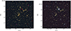 |
Fig. 1. Extract of the field of view analysed centred on the galaxy cluster Abell 2744 as observed at the two facilities. The left panel depicts a colour composite Subaru/Suprime-Cam BRcz′ image; the right panel is the colour composite Magellan/MegaCam gri image. |
Specifics of the observations performed with the Subaru/Suprime-Cam and the Magellan/MegaCam cameras.
3.2. Source identification
We first identified the astronomical sources located in the field of view with the SExtractor software (Bertin & Arnouts 1996) in the dual-image mode. The detections were carried out on the Magellan/MegaCam gri composite image, because of their superior depth and resolution, whereas the measurements of the physical properties of the sources (e.g. size and magnitude) were performed on the single-band images individually. A total of 11 7001 sources were thus recognised. We later classified them as galaxies and stars in the three bands independently, by studying their distribution in size and magnitude. As a reference for the size of the objects we used the flux radius measured by SExtractor (i.e. the radius of the isophote enclosing 40% of the total luminosity of the source). In a magnitude-size diagram, stars occupy a well-defined vertical region of approximately constant radius, whereas galaxies are broadly distributed in both size and flux. After removing the sources associated with saturated pixels, we identified as galaxies those objects recognised as such in at least one of the three bands and that were not classified either as stars or as saturated objects in the other filters. A similar procedure was followed to identify the stars. In our field of view we thus identified 695 objects as stars and 86 945 as galaxies. This corresponds to an average number density of ≃84 galaxies/arcmin−2. Figure 2 shows the distribution in size and magnitude of both stars and galaxies in the g band; similar results were found for the other filters. It is worth mentioning the lack of the ‘brighter-fatter’ effect up to magnitude 19, as emerges from Fig. 2: the region occupied by the unsaturated stars is vertical (i.e. they have an approximately constant flux radius irrespective of their luminosity). Saturated stars have been explicitly ignored in our analysis and are shown as grey dots in Fig. 2.
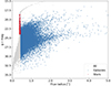 |
Fig. 2. Classification of the sources between galaxies (blue) and stars (red) after the comparison of the three bands from the Magellan data, as illustrated in the text, in a magnitude–size diagram. Also shown are all the detected sources (in grey). The values of the magnitude and flux radius reported here refer to the g band. |
3.3. Identification of cluster and background galaxies
Afterwards, we distinguished the galaxies between cluster members and background members by adopting the procedure outlined by Medezinski et al. (2010, 2018) and successfully applied in several WL analyses of galaxy clusters (see e.g. Jauzac et al. 2012; Medezinski et al. 2013, 2016). We produced a colour–colour (CC) g − r versus r − i diagram (left panel of Fig. 3) and evaluated the mean distance of all the galaxies from the cluster centre in a given CC cell (right plot in Fig. 3). We considered as the centre of the system the brightest cluster galaxy (BCG). The upper central region (identified by the white contours in both panels) is mainly populated by galaxies having the smallest mean distance from the centre of the cluster. It can be seen that this region corresponds to a local overdensity in the CC space. We therefore selected the galaxies residing in this region as potential cluster members, and further restricted the choice to those lying within 1.2 Mpc (i.e. 6′ at the redshift of the cluster) of the centre of the image. We identified in this way 1477 galaxies likely belonging to the cluster. These galaxies occupy a well-defined red cluster sequence in the colour-magnitude diagram depicted in Fig. 4.
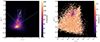 |
Fig. 3. Distribution of the identified galaxies in a colour–colour diagram. The left panel is the colour–colour (CC) diagram g − r vs. r − i, whereas the right panel displays the distribution of the mean distances of the galaxies from the centre of the image in the same space. The rectangular box identified with the white lines in both panels identifies the region where the cluster was estimated to lie in the CC space. In the left panel the white dots identify the 201 spectroscopically confirmed cluster members. The cyan lines in the left panel denote the region below which the background galaxies are assumed to lie. |
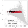 |
Fig. 4. Colour–magnitude diagram g − i vs. i for all the galaxies (grey) and for those we identified as cluster members (red). The latter define a clearly visible red cluster sequence. The black crosses identify the 201 spectroscopically confirmed cluster members. |
We verified the purity and completeness of our cluster sample by comparing it to the spectroscopic redshift catalogue used by Bergamini et al. (2023a), who performed a SL study of the same galaxy cluster based on JWST/NIRCam imaging and VLT Multi Unit Spectroscopic Explorer (MUSE) spectroscopy. The catalogue contains the spectroscopic redshifts of 2397 objects from Braglia et al. (2009), Owers et al. (2011), and Richard et al. (2021). To make a fair comparison with our sample, we considered only the galaxies lying in the redshift range (0.28, 0.34) (which corresponds to a rest-frame velocity of the galaxies in the cluster of ±6000 km s−1 around the median redshift of the cluster) and within 6′ from the cluster centre. Out of the 710 galaxies present in both datasets, 201 of them were classified by the authors as cluster members and satisfied the distance criterion described above, and we correctly identified 150 of them. We quantified the goodness of our classification by estimating the purity and the completeness, defined as
 (8)
(8)
and
 (9)
(9)
Here, TP, FP, and FN denote the true positives, false positives, and false negatives, respectively. We achieved a purity of ≃84% and a completeness of ≃87%. The spectroscopically confirmed cluster members are depicted as white dots in the left panel of Fig. 3.
With the 1477 galaxies selected above to be potential cluster members, we reconstructed the surface brightness distribution of the cluster. We took into account the K-correction (Hogg et al. 2002) by following the procedure in Beare et al. (2014), which allowed us to express the K-corrected magnitudes as a suitable combination of the available colours. The luminosity distribution in the K-corrected r band is depicted in Fig. 5, where the contour lines of the recovered surface mass density (see below) are also overlaid.
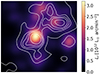 |
Fig. 5. 7′×7′ extract of the surface brightness distribution of the cluster in the K-corrected r band, with overlaid (in white), the contours of the total surface mass distribution at 2.5, 5, 6, 7 and 9 σk (see Sect. 4). |
Finally, we isolated the foreground galaxies from the background galaxies by identifying the region corresponding to an absolute maximum in the galaxy number density in the centre of the CC diagram (left panel of Fig. 3), which is mainly populated by foreground sources: we thus obtained a catalogue consisting of 54 614 potential background galaxies. The cyan lines in the left panel of Fig. 3 denote the region below which we assumed the background galaxies to lie.
4. WL analysis
4.1. PSF reconstruction
Before measuring the ellipticities of the background galaxies, we reconstructed the spatial variation of the point spread function (PSF) all over the field of view. The PSF introduces an artificial shape distortion, which has to be accurately measured and properly corrected for. For this purpose, we used mccd (Liaudat et al. 2021), a module of the pipeline shapepipe (Guinot et al. 2022; Farrens et al. 2022) we applied to our WL analysis. Unlike other software programs, mccd is capable of handling multiple CCDs simultaneously, thus handling discontinuities at the CCD boundaries and providing a single continuous PSF field, instead of producing a PSF model for each CCD separately. The point spread function is described by the software in terms of a model, specified by the user, split into a global and a local term. The latter describes the PSF variation over a single CCD as a function of the pixel coordinates, whereas the former takes into account all the CCDs. The mccd package operates on stamps of the stars to measure their shapes and thus determine the parameters of the model, which are later interpolated at the coordinates of the galaxies. In our work, both the global and the local terms coincided since, in order to simplify the WL pipeline, we directly operated on the single-band co-added images instead of working on individual frames. This may result in a limitation in the use of the code; however, we opted for a less complex methodology, and given the results we obtained (see below), we are satisfied with the results obtained with mccd. We applied the software on the three single-images separately, and obtained three different PSF maps.
We quantified the goodness of our PSF reconstruction by measuring the difference between the ellipticity ε = ε1 + iε2 of the observed stars and the that obtained after correcting for the PSF reconstruction at the same locations. The result is depicted in Fig. 6, and shows the ellipticity distribution before (black) and after (red) the PSF correction, as well as the position of the means of the distributions (in white and black, respectively) obtained with the Python-based huber estimator (Huber 1964). The results obtained with both the Subaru/Suprime-Cam (left panel) and the Magellan/MegaCam (right panel) cameras are shown. For the Magellan results, before correcting for the PSF, we estimated mean values of ⟨ε1⟩before = ( − 0.95 ± 9.28)×10−3 and ⟨ε2⟩before = (0.69 ± 1.37)×10−2. After the correction, we recovered mean values of ⟨ε1⟩after = (0.59 ± 1.06)×10−3 and ⟨ε2⟩after = (0.46 ± 1.53)×10−3.
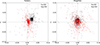 |
Fig. 6. Ellipticity distribution of the stars on the field of view before (in black) and after (in red) the PSF correction. The white (black) cross represents the mean of the distribution before (after) the correction. The left (right) panel shows the results for the Subaru (Magellan, respectively) facility. |
4.2. Shear measurement
We thus proceeded with the measurements of the shapes of the background galaxies with the module ngmix (Sheldon 2015; Sheldon & Huff 2017) of the above-mentioned shapepipe pipeline, which follows a model-fitting approach. For each galaxy, a stamp centred on it must be supplied. We used a square box with a size of six times the highest value of the flux radius (among the three bands) corresponding to that galaxy. The algorithm first fits the PSF associated with it (which was reconstructed in the previous passage) as a mixture of m co-axial Gaussian distributions, with the integer m specified by the user. Afterwards, the galaxy shape is measured: galaxies are initially described in terms of a parametrised surface brightness distribution; later, the resulting image is sheared and the previously fitted PSF is applied. Then, ngmix applies a least-squares method based on the Levenberg–Marquardt algorithm to fit the original image with the model, and returns the best-fit model parameters, including the two components of the shear. This operation is run once, and then the process is bootstrapped several times, such that an entire strip of best-fit values is returned, as well as their standard deviations and covariance matrix. Throughout the analysis, we set m = 2 and adopted a simple exponential surface brightness profile to model the galaxies since we were only interested in their shapes. Before opting for this choice, we had run ngmix both on simulated galaxies and on Subaru/Suprime-Cam data by using different models. Extensive tests on different combinations of galaxy shapes have shown that, for galaxies with angular sizes not much larger than the PSF size, as in our situation, a fit consisting of a single exponential profile is much more robust and reliable than a fit obtained by using a combination of exponential and de Vaucouleurs profiles. This is likely associated with the presence of degeneracies when a limited amount of information is available. Therefore, we opted for a pure exponential profile.
This algorithm does not measure the galaxy shapes correctly if the image provided to the software contains two or more objects, since it is not capable of disentangling multiple profiles. Therefore, we initially removed from our background sample the galaxies with overlapping isophotes, by exploiting the segmentation map produced by SExtractor. Furthermore, we removed from the subsequent analysis the galaxies lying close to bad and/or saturated pixels, stars of our Galaxy, and the edges of the field of view. We therefore applied ngmix to measure the shape of the 20 519 remaining background galaxies. To do so, we adopted the multi-band configuration (i.e. the measurements were carried out on an image created by stacking three stamps of each galaxy in the three filters individually). For each galaxy, the stamp was obtained on the three mosaic co-added images corresponding to the three different filters. We also supplied each single-band stamp with a corresponding box in the weight map and in the PSF map. In the case of galaxies with a signal-to-noise ratio (S/N) of less than 10 measured by SExtractor in a given band, the weight box in that filter was set to zero when creating the multi-band stamp, so as to force the algorithm not to use that filter.
After these measurements, we further cleaned our sample before reconstructing the shear field all over the field of view. We removed the galaxies whose shear components were measured with a standard deviation higher than 0.7, those whose centre (as measured with SExtractor) differed from that fitted with ngmix by more than 0.75″, and those with a S/N of less than 10 evaluated by the algorithm. This left us with Nb = 13 942 background galaxies to compute the total mass distribution with, corresponding to ≃15 galaxies/arcmin2. We thus reconstructed the shear field γ(x) by applying Eq. (3). To do so, we pixelised the field of view onto a 480 px × 500 px grid (corresponding to a pixel scale of 0.1′) and introduced an isotropic two-dimensional Gaussian weight function K with standard deviation equal to 0.5′. We evaluated the dispersion on the intrinsic ellipticity appearing in Eq. (4) by using our shape measurements, as
 (10)
(10)
where for each galaxy  is given by the sum in quadrature of the uncertainties of the two components of the ellipticity returned by ngmix. We obtained σε = 0.25. The weights {⟨Z⟩n} and {⟨Z2⟩n} appearing in Eq. (3), as suggested previously, depend on the redshift distribution of the background galaxies. Since we did not have this information at our disposal, we proceeded in the following way to evaluate them. We derived the redshift distribution from the photometric redshift catalogue centred in the Hubble Deep Field-North by Yang et al. (2014). We first selected the sources in the catalogue recognised as galaxies, and then applied the same selection criteria described in the previous section to determine the background galaxies. If zj denotes the redshift of the jth catalogue galaxy with magnitude m in the interval [mi, mi + 0.5) in a given band and Ni the number of catalogue galaxies in the same bin, we evaluated the ⟨Z⟩i and the ⟨Z2⟩i corresponding to the ith bin by using the equations
 (11)
(11)
and
 (12)
(12)
In the previous equations, Σcr, ∞ is the critical surface mass distribution given in Eq. (2) for a fictitious source at infinite redshift. We thus assigned each of our background galaxies having a magnitude in the ith bin the corresponding ⟨Z⟩i and ⟨Z2⟩i values. As a reference band, we opted for the r filter. Typical values of the variance of ⟨Z⟩i and ⟨Z2⟩i are around unity for all magnitude bins.
4.3. Cluster mass reconstruction
We thus reconstructed the convergence κ and then the total surface mass distribution Σ through Eq. (5), by applying Eq. (7). We first constructed G and then solved the linear equation using a least-squares method to obtain κ, and hence Σ. We applied the iterative procedure described in Seitz & Schneider (1995), which reached convergence in five steps. We also estimated a statistical error σk on the reconstruction of Σ through a reshuffling procedure (Lombardi & Bertin 1999); in other words, we produced 120 additional mass density maps, each time shuffling the coordinates of the background galaxies, and then evaluated the rms error σk on the resulting 120 realisations of Σ. Figure 7 depicts the contour levels of Σ over the central 6′×6′ region of the g-band image.
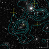 |
Fig. 7. Central 6′×6′ region of the g-band image with overlaid the contour levels of the total surface mass distribution at 2.5, 5, 6, 7, and 9 σk. The yellow crosses denote the density peaks identified by Medezinski et al. (2016). |
We further looked for potential systematic effects by evaluating the B-modes. The two components of the shear can indeed be decomposed into two parts, the E- (curl-free) and the B- (divergence-free) modes. In the context of gravitational lensing, the E-mode signal is related to the surface mass distribution, whereas the B-mode signal is identically zero (Umetsu 2020). The presence of non-null B-modes can thus be used as a test for the presence of systematic effects. To do so, we evaluated the lensing signal Σ after rotating each component of the shear of an angle equal to π/4 (i.e. mapping γ1 → −γ2 and γ2 → γ1). We followed the same procedure outlined above, and then estimated the rms error on the distribution found in this way by means of a similar reshuffling procedure. The resulting B-mode thus obtained is consistent with zero.
Finally, as in all WL analyses, our mass reconstruction is affected by the mass-sheet degeneracy (i.e. Σ can be determined up to an additive constant c) (for a review, see again Bartelmann & Schneider 2001). As can be seen in Eq. (5), an additive constant does not modify the gradient, and therefore the minimisation of the action. To deal with this degeneracy and obtain an estimate of c, we modelled the main density peak of our surface mass distribution (the one in the south-east part of the cluster; see below) in terms of a simple softened isothermal ellipsoid (SIE; Keeton 2001), depending, among other parameters, on the additive constant c.
To determine the free parameters of the model, λ, we performed a Bayesian inference. We expressed the likelihood as the product of bi-dimensional Gaussian distributions  , where Σ(x) and Σ0(x|λ) are the reconstructed and modelled total surface mass distributions given the parameters λ at location x, respectively, and
  is the value of the variance map at the same coordinate. We only restricted to the annulus with internal radius equal to ∼3 Mpc and external radius equal to ∼4 Mpc, where the radial density profile of the cluster is supposed to vanish. We inferred the parameters assuming as a prior a uniform distribution over a suitable subset in the parameter space. In particular, we left c free to vary in the interval [ − 1, 1]×1015 M⊙/Mpc2. We sampled the posterior distribution with the nested sampling Monte Carlo algorithm Ultranest (Buchner 2021). We found c = (4 ± 1)×1012 M⊙/Mpc2. Figure 8 shows the cumulative mass profiles, obtained by averaging the surface mass distribution on circular apertures. We adopted as the centre of the mass profile the centre of the cluster indicated at the end of Sect. 1. The plot also depicts the results from the preliminary WL analysis carried out on Subaru/Suprime-Cam BRcz′ data, on which we first applied the pipeline described above.
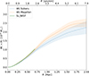 |
Fig. 8. Cumulative radial total mass profile of the cluster obtained with Subaru/Suprime-Cam (blue) and Magellan/Megacam (orange) imaging. Also shown is the cumulative profile (green) in the core of the cluster as a result of the SL analysis based on JWST (Bergamini et al. 2023b). The shaded area denotes the error band corresponding to the 68% confidence level. |
5. Discussion and results
5.1. Comparison between strong lensing and weak lensing
In the previous sections we presented the WL analysis that we performed to reconstruct the total mass distribution of the galaxy cluster Abell 2744. At a distance of 2.35 Mpc from the south-east BCG, we recovered a total mass of (2.56 ± 0.26)×1015 M⊙, which is slightly higher than the previous WL study of the same cluster by Medezinski et al. (2016), who found a value of the total mass within the same aperture of (2.06 ± 0.42)×1015 M⊙, albeit consistent within one rms. Moreover, the total mass enclosed within 1 Mpc, equal to (1.68 ± 0.13)×1015 M⊙, is in very good agreement with the estimate obtained by Boschin et al. (2006), equal to (1.4 − 2.4)×1015 M⊙ within the same radius, who performed a dynamical analysis of the cluster based on New Technology Telescope (NTT) European Southern Observatory (ESO) Multimode Instrument (EMMI, D’Odorico 1990) spectrography. Additionally, our result is consistent with the finding of the above-mentioned combined SL-WL analysis by Jauzac et al. (2016): they found a total mass enclosed within 1.3 Mpc from the BCG equal to (2.3 ± 0.1)×1015 M⊙, which is perfectly consistent with the total mass enclosed within the same radius we found, (2.1 ± 0.2)×1015 M⊙. To further corroborate the validity of our results, we compared our findings with the SL study by Bergamini et al. (2023b) based on new deep, high-resolution JWST imaging, after extrapolating their best-fit model up to 700 kpc. To make a fair comparison between the outcomes from the two different probes, we downgraded the best-fit SL surface mass distribution to the same resolution of our WL map. We then estimated the uncertainty on it by evaluating an additional 120 maps using different combinations of randomly extracted parameters from the SL model MCMC chains and evaluating the rms error. As can be seen in Fig. 9, where both the best-fit SL model and the WL surface mass distributions are overlaid on a JWST rgb composite image, a good agreement emerges for the southern and the right north-west density peaks. Only a slight discrepancy in the left north-west peak is present, likely due to the presence of a saturated star in the Magellan images (also visible in the JWST composite image), which we had to suitably mask out, and thus losing shape information about the galaxies located in its neighbourhood. We note that our WL study is capable of extrapolating the SL map out to large radii (up to a few Mpc). As a further test, we evaluated the radial cumulative mass distribution from the SL probe by following the same procedure outlined above for the WL analysis (see Fig. 8). Our findings are clearly in excellent agreement within one σk.
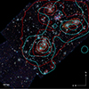 |
Fig. 9. Central 900 kpc × 900 kpc region of the composite JWST rgb image with overlaid the contour levels of the surface mass distribution emerging from the SL (Bergamini et al. 2023b, in red) and our WL (in cyan) studies. The contour levels depicted are linearly spaced between 0.5 × 10¹⁵ M⊙/Mpc2 and 2.4 × 10¹⁵ M⊙/Mpc2. |
Furthermore, our analysis reveals the presence of three density peaks having a S/N greater than 7: one peak, with higher density and a S/N of 14.0, lies in the south-east part of the cluster very close to the BCG, whereas the others are found in the north-west corner. All of them lie close to those observed in the SL surface mass distribution by Bergamini et al. (2023b). A slight overlap with the locations of the substructures detected in the WL study by Medezinski et al. (2016) (yellow crosses in Fig. 7) is also observed. In particular, the south-east substructre detected in Medezinski et al. (2016) lies well within our density peak, as does the north-west structure. This result suggests that the cluster is not relaxed, but is undergoing a complex merging process, as supported by the previously mentioned papers.
5.2. Comparison between mass and luminosity distributions
We compared the recovered surface mass distribution with the luminosity density of the cluster, as represented in Fig. 5. As can be seen, there is a nice agreement between mass and luminosity, except for a slight misalignment for the north-west density peak. We explain this discrepancy as a consequence of the above-mentioned effect due to the presence of the star we had to mask out. Furthermore, we estimated a mass-to-light ratio M/L in the K-corrected r band as the ratio of the total mass to the total luminosity Lr within 200 kpc; we found M(< 250 kpc)/Lr(< 250 kpc) = 573 ± 69 M⊙/L⊙, r, which is perfectly consistent with the results found by Medezinski et al. (2016) with Subaru imaging.
5.3. Comparison between Subaru and Magellan
In the previous sections we presented the results obtained with Magellan/MegaCam, after we tested both mccd and ngmix on the Subaru dataset, although the latter is characterised by a worse PSF and depth. These features therefore impacted the quality of the analysis. Firstly, with Subaru/Suprime-Cam, we detected fewer galaxies, as can be seen in Fig. 10, which displays the number counts per unit area referred to two filters, Rc and r for Subaru and Magellan, respectively. In particular, after applying the same CC method described previously, the average number density of background sources was slightly less than half of that with Magellan (≃33 galaxies/arcmin2). Moreover, after removing the galaxies unsuitable for the WL analysis, this density lowered to ≃9 galaxies/arcmin2. Secondly, we reported a significant difference for the shape measurements. For the Subaru dataset only, we found a significant fraction of background galaxies with an ellipticity measured by ngmix higher than 0.97 and an error on both the components of ε higher than unity, and thus indicating the failure in fitting the galaxy shape due to the low S/N. Additionally, ngmix fails to measure, with a sufficiently low error, the shape of faint galaxies, as emerges from Fig. 11. The median error on ε indeed increases with the apparent magnitude of the galaxies, with the errors on the Subaru imaging being steadily higher than those with Magellan imaging data. We therefore had to remove these sources from the subsequent analysis, which thus led to a result that was slightly different from that obtained with Magellan. At a distance of 2 Mpc from the BCG, the total mass is slightly lower, (2.41 ± 0.47)×1015 M⊙, and characterised by a rms almost twice that obtained with Magellan. Nevertheless, the two results agree with each other within one rms, as emerges from Fig. 8.
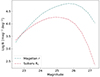 |
Fig. 10. Number counts of the galaxies per unit area and magnitude for the Subaru (red) Rc band and the Magellan (blue) r filter. |
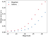 |
Fig. 11. Distribution of the median error on the ellipticity as a function of the apparent magnitude of the background galaxies, for the Magellan (blue) and the Subaru (red) datasets. |
5.4. Data contamination
The results we obtained depend on several factors. Firstly, we classified the galaxies between cluster members, and foreground and background members, by studying their distribution only in a CC space. An erroneous classification could lead to a dilution in the WL signal, and therefore influence the outcome of our analysis. We took care of this systematic by verifying the correctness of our classification through a comparison with the spectroscopic redshift catalogue by Bergamini et al. (2023a). Out of the galaxies present in both catalogues, we correctly identified the background sources with a purity of ≃70%. It should be noted, however, that the VLT/MUSE catalogue was obtained by analysing an area of few square arcmin, whereas our field of view covered an area of approximately 0.3 deg2. To overcome this bias, it would be useful for future WL works the use of multi-band imaging data obtained from several bands in order to estimate photometric redshifts, and thus allowing for a complementary method for the classification. These redshifts would also allow one to estimate the critical surface mass density in Eq. (2) for each background galaxy. This would lead to a more robust mass reconstruction.
Similarly, we propose the use of other techniques, including the application of convolutional neural networks (CNNs) (LeCun et al. 1989, 1998). These algorithms are composed of several convolutional layers that are able to recognise complex features within the images on which they are applied. Recent works show how the CNNs are capable of achieving a high (> 90%) purity-completeness rate when tested on multi-band imaging data (see Angora et al. 2020), and thus making their application in upcoming WL studies promising.
6. Conclusions
We have presented a WL analysis of the galaxy cluster Abell 2744 using new deep multi-band gri imaging from Magellan/Megacam. For our study we applied a pipeline based on two brand-new programs, mccd and ngmix, for the PSF reconstruction and shape measurement, respectively. Unlike previous algorithms developed for this scope, both mccd and ngmix allow one to exploit the information from all the bands simultaneously. Moreover, mccd is capable of modelling the spatial variation of the point spread function of several CCDs, and thus avoiding potential discontinuities at the boundaries. To test the robustness of these algorithms, we first applied them on multi-band BRcz′ Subaru/Suprime-Cam imaging of the same cluster, covering an effective field of view of ≃24′×27′, and with a depth of ≃27.9 in the B band. Afterwards, we analysed the deeper (up to mlim = 28.7 in the g band) and larger (≃31′×33′) Magellan/MegaCam dataset. We performed a robust analysis by carefully isolating the background galaxies, thus taking care of possible contaminations in the WL signal, which is one of the main sources of systematic uncertainties. We further verified the purity and completeness of our sample by using a reference spectroscopic redshift catalogue based on VLT/MUSE data centred on the same cluster. The reconstructed total surface mass distribution reveals the presence of three density peaks in the inner core of the cluster with significance greater than 7σk, thus supporting the hypothesis of a complex merging phenomenon from previous studies of the same cluster realised with different probes (e.g. galaxy dynamics) and performed in several bands (e.g. X-ray and radio). This picture is also confirmed by a comparison with a new high-precision SL JWST-based analysis of the central region of the cluster, with which we found a nice agreement. Not only do the two surface mass distributions resulting from the two methods agree, but our cumulative total mass profile is also consistent within the errors with the SL profile, over the radial range where they overlap. The total mass enclosed within 2.35 Mpc is (2.56 ± 0.26)×1015 M⊙, which is consistent with previous WL analyses of the same cluster and with different probes, for example dynamical methods, thus making Abell 2744 one of the most massive galaxy clusters ever studied.
Acknowledgments
The authors thank the anonymous referee for the useful comments that helped to improve the manuscript. This paper includes data gathered with the 6.5 meter Magellan Telescopes located at Las Campanas Observatory, Chile. The authors thank Amata Mercurio and Tommaso Treu for proposing us to perform an analysis of Abell 2744 with Magellan/MegaCam data to complement the SL JWST-based study by Bergamini et al. (2023b). We also thank useful discussions with Erin Sheldon about his software ngmix.
References
- Angora, G., Rosati, P., Brescia, M., et al. 2020, A&A, 643, A177 [NASA ADS] [CrossRef] [EDP Sciences] [Google Scholar]
- Atek, H., Chemerynska, I., Wang, B., et al. 2023a, MNRAS, 524, 5486 [NASA ADS] [CrossRef] [Google Scholar]
- Atek, H., Shuntov, M., Furtak, L. J., et al. 2023b, MNRAS, 519, 1201 [Google Scholar]
- Bartelmann, M., & Schneider, P. 2001, Phys. Rep., 340, 291 [Google Scholar]
- Beare, R., Brown, M., & Pimbblet, K. 2014, ApJ, 797, 104 [NASA ADS] [CrossRef] [Google Scholar]
- Bergamini, P., Rosati, P., Mercurio, A., et al. 2019, A&A, 631, A130 [NASA ADS] [CrossRef] [EDP Sciences] [Google Scholar]
- Bergamini, P., Acebron, A., Grillo, C., et al. 2023a, A&A, 670, A60 [NASA ADS] [CrossRef] [EDP Sciences] [Google Scholar]
- Bergamini, P., Acebron, A., Grillo, C., et al. 2023b, ApJ, 952, 84 [NASA ADS] [CrossRef] [Google Scholar]
- Bertin, E., & Arnouts, S. 1996, A&AS, 117, 393 [NASA ADS] [CrossRef] [EDP Sciences] [Google Scholar]
- Bertin, E., Mellier, Y., Radovich, M., et al. 2002, ASP Conf. Proc., 281, 228 [NASA ADS] [Google Scholar]
- Bezanson, R., Labbe, I., Whitaker, K. E., et al. 2022, ApJ, submitted, [arXiv:2212.04026] [Google Scholar]
- Boschin, W., Girardi, M., Spolaor, M., & Barrena, R. 2006, A&A, 449, 461 [NASA ADS] [CrossRef] [EDP Sciences] [Google Scholar]
- Braglia, F. G., Pierini, D., Biviano, A., & Boehringer, H. 2009, VizieR Online Data Catalog, J/A+A/500/947 [Google Scholar]
- Buchner, J. 2021, J. Open Source Software, 6, 60 [Google Scholar]
- Cha, S., HyeongHan, K., Scofield, Z. P., Joo, H., & Jee, M. J. 2024, ApJ, 961, 186 [NASA ADS] [CrossRef] [Google Scholar]
- Chen, W., Kelly, P., Broadhurst, T., et al. 2022a, Transient Name Server AstroNote, 260, 1 [NASA ADS] [Google Scholar]
- Chen, W., Kelly, P., Castellano, M., et al. 2022b, Transient Name Server AstroNote, 257, 1 [NASA ADS] [Google Scholar]
- Clowe, D., Bradač, M., Gonzalez, A. H., et al. 2006, ApJ, 648, L109 [NASA ADS] [CrossRef] [Google Scholar]
- Coe, D., Umetsu, K., Zitrin, A., et al. 2012, ApJ, 757, 22 [NASA ADS] [CrossRef] [Google Scholar]
- David, L. P., Jones, C.& Forman, W. 1995, ApJ, 445, 578 [NASA ADS] [CrossRef] [Google Scholar]
- D’Odorico, S. 1990, The Messenger, 61, 51 [Google Scholar]
- Farrens, S., Guinot, A., Kilbinger, M., et al. 2022, A&A, 664, A141 [NASA ADS] [CrossRef] [EDP Sciences] [Google Scholar]
- Giovannini, G., Tordi, M., & Feretti, L. 1999, New Astron., 4, 141 [CrossRef] [Google Scholar]
- Govoni, F., Enßlin, T. A., Feretti, L., & Giovannini, G. 2001a, A&A, 369, 441 [NASA ADS] [CrossRef] [EDP Sciences] [Google Scholar]
- Govoni, F., Feretti, L., Giovannini, G., et al. 2001b, A&A, 376, 803 [CrossRef] [EDP Sciences] [Google Scholar]
- Grillo, C., Suyu, S. H., Rosati, P., et al. 2015, ApJ, 800, 38 [Google Scholar]
- Guinot, A., Kilbinger, M., Farrens, S., et al. 2022, A&A, 666, A162 [NASA ADS] [CrossRef] [EDP Sciences] [Google Scholar]
- Hoekstra, H., Franx, M., & Kuijken, K. 2000, ApJ, 532, 88 [Google Scholar]
- Hogg, D. W., Baldry, I. K., Blanton, M. R., & Eisenstein, D. J. 2002, arXiv e-prints [arXiv:astro-ph/0210394] [Google Scholar]
- Huber, P. J. 1964, Ann. Math. Stat., 35, 492 [Google Scholar]
- Jauzac, M., Jullo, E., Kneib, J.-P., et al. 2012, MNRAS, 426, 3369 [Google Scholar]
- Jauzac, M., Eckert, D., Schwinn, J., et al. 2016, MNRAS, 463, 3876 [NASA ADS] [CrossRef] [Google Scholar]
- Kaiser, N., & Squires, G. 1993, ApJ, 404, 441 [Google Scholar]
- Keeton, C. R. 2001, arXiv e-prints [arXiv:astro-ph/0102341] [Google Scholar]
- Kempner, J. C., & David, L. P. 2004, MNRAS, 349, 385 [NASA ADS] [CrossRef] [Google Scholar]
- LeCun, Y., Boser, B., Denker, J., Henderson, D., et al. 1989, Neural Comput., 1, 541 [NASA ADS] [CrossRef] [Google Scholar]
- LeCun, Y., Bottou, L., Bengio, Y., & Haffner, P. 1998, Proc. IEEE, 86, 2278 [Google Scholar]
- Le Fèvre, O., Saisse, M., Mancini, D., et al. 2003, in Instrument Design and Performance for Optical/Infrared Ground-based Telescopes, eds. M. Iye, & A. F. M. Moorwood, SPIE Conf. Ser., 4841, 1670 [CrossRef] [Google Scholar]
- Liaudat, T., Bonnin, J., Starck, J. L., et al. 2021, A&A, 646, A27 [NASA ADS] [CrossRef] [EDP Sciences] [Google Scholar]
- Lombardi, M., & Bertin, G. 1998, A&A, 330, 791 [NASA ADS] [Google Scholar]
- Lombardi, M., & Bertin, G. 1999, A&A, 348, 38 [NASA ADS] [Google Scholar]
- Lombardi, M., Rosati, P., Nonino, M., et al. 2000, A&A, 363, 401 [NASA ADS] [Google Scholar]
- Lotz, J. 2013, HST Frontier Fields - Observations of Abell 2744, HST Proposal ID 13495. Cycle 21 [Google Scholar]
- Lotz, J. M., Koekemoer, A., Coe, D., et al. 2017, ApJ, 837, 97 [Google Scholar]
- McLeod, B., Geary, J., Conroy, M., et al. 2015, PASP, 127, 366 [NASA ADS] [CrossRef] [Google Scholar]
- Medezinski, E., Broadhurst, T., Umetsu, K., et al. 2010, MNRAS, 405, 257 [NASA ADS] [Google Scholar]
- Medezinski, E., Umetsu, K., Nonino, M., et al. 2013, ApJ, 777, 43 [NASA ADS] [CrossRef] [Google Scholar]
- Medezinski, E., Umetsu, K., Okabe, N., et al. 2016, ApJ, 817, 24 [NASA ADS] [CrossRef] [Google Scholar]
- Medezinski, E., Oguri, M., Nishizawa, A. J., et al. 2018, PASJ, 70, 30 [NASA ADS] [Google Scholar]
- Merten, J., Coe, D., Dupke, R., et al. 2011, MNRAS, 417, 333 [NASA ADS] [CrossRef] [Google Scholar]
- Miyazaki, S., Komiyama, Y., Sekiguchi, M., et al. 2002, PASJ, 54, 833 [Google Scholar]
- Niemiec, A., Jauzac, M., Eckert, D., et al. 2023, MNRAS, 524, 2883 [NASA ADS] [CrossRef] [Google Scholar]
- Nonino, M., Dickinson, M., Rosati, P., et al. 2009, ApJS, 183, 244 [NASA ADS] [CrossRef] [Google Scholar]
- Owers, M. S., Randall, S. W., Nulsen, P. E. J., et al. 2011, ApJ, 728, 27 [Google Scholar]
- Paris, D., Merlin, E., Fontana, A., et al. 2023, ApJ, 952, 20 [CrossRef] [Google Scholar]
- Postman, M., Coe, D., Benítez, N., et al. 2012, ApJS, 199, 25 [Google Scholar]
- Pratt, G. W., Arnaud, M., Biviano, A., et al. 2019, Space. Sci. Rev., 215, 25 [NASA ADS] [CrossRef] [Google Scholar]
- Richard, J., Claeyssens, A., Lagattuta, D., et al. 2021, VizieR Online Data Catalog, J/A+A/646/A83. [Google Scholar]
- Roberts-Borsani, G., Treu, T., Chen, W., et al. 2023, Nature, 618, 480 [NASA ADS] [CrossRef] [Google Scholar]
- Rosati, P., Balestra, I., Grillo, C., et al. 2014, The Messenger, 158, 48 [NASA ADS] [Google Scholar]
- Seitz, C., & Schneider, P. 1995, A&A, 297, 287 [NASA ADS] [Google Scholar]
- Sheldon, E. 2015, Astrophysics Source Code Library [record ascl:1508.008] [Google Scholar]
- Sheldon, E. S., & Huff, E. M. 2017, ApJ, 841, 24 [NASA ADS] [CrossRef] [Google Scholar]
- Steinhardt, C. L., Jauzac, M., Acebron, A., et al. 2020, ApJS, 247, 64 [Google Scholar]
- Treu, T., Roberts-Borsani, G., Bradac, M., et al. 2022, ApJ, 935, 110 [NASA ADS] [CrossRef] [Google Scholar]
- Umetsu, K. 2020, A&A Rev., 28, 7 [NASA ADS] [CrossRef] [Google Scholar]
- Umetsu, K., Medezinski, E., Broadhurst, T., et al. 2010, ApJ, 714, 1470 [NASA ADS] [CrossRef] [Google Scholar]
- Umetsu, K., Broadhurst, T., Zitrin, A., Medezinski, E., & Hsu, L.-Y. 2011, ApJ, 729, 127 [NASA ADS] [CrossRef] [Google Scholar]
- Umetsu, K., Medezinski, E., Nonino, M., et al. 2014, ApJ, 795, 163 [NASA ADS] [CrossRef] [Google Scholar]
- Umetsu, K., Ueda, S., Hsieh, B.-C., et al. 2022, ApJ, 934, 169 [NASA ADS] [CrossRef] [Google Scholar]
- Yang, G., Xue, Y. Q., Luo, B., et al. 2014, ApJS, 215, 27 [NASA ADS] [CrossRef] [Google Scholar]
All Tables
Specifics of the observations performed with the Subaru/Suprime-Cam and the Magellan/MegaCam cameras.
All Figures
|
Fig. 1. Extract of the field of view analysed centred on the galaxy cluster Abell 2744 as observed at the two facilities. The left panel depicts a colour composite Subaru/Suprime-Cam BRcz′ image; the right panel is the colour composite Magellan/MegaCam gri image. |
| In the text | |
|
Fig. 2. Classification of the sources between galaxies (blue) and stars (red) after the comparison of the three bands from the Magellan data, as illustrated in the text, in a magnitude–size diagram. Also shown are all the detected sources (in grey). The values of the magnitude and flux radius reported here refer to the g band. |
| In the text | |
|
Fig. 3. Distribution of the identified galaxies in a colour–colour diagram. The left panel is the colour–colour (CC) diagram g − r vs. r − i, whereas the right panel displays the distribution of the mean distances of the galaxies from the centre of the image in the same space. The rectangular box identified with the white lines in both panels identifies the region where the cluster was estimated to lie in the CC space. In the left panel the white dots identify the 201 spectroscopically confirmed cluster members. The cyan lines in the left panel denote the region below which the background galaxies are assumed to lie. |
| In the text | |
|
Fig. 4. Colour–magnitude diagram g − i vs. i for all the galaxies (grey) and for those we identified as cluster members (red). The latter define a clearly visible red cluster sequence. The black crosses identify the 201 spectroscopically confirmed cluster members. |
| In the text | |
|
Fig. 5. 7′×7′ extract of the surface brightness distribution of the cluster in the K-corrected r band, with overlaid (in white), the contours of the total surface mass distribution at 2.5, 5, 6, 7 and 9 σk (see Sect. 4). |
| In the text | |
|
Fig. 6. Ellipticity distribution of the stars on the field of view before (in black) and after (in red) the PSF correction. The white (black) cross represents the mean of the distribution before (after) the correction. The left (right) panel shows the results for the Subaru (Magellan, respectively) facility. |
| In the text | |
|
Fig. 7. Central 6′×6′ region of the g-band image with overlaid the contour levels of the total surface mass distribution at 2.5, 5, 6, 7, and 9 σk. The yellow crosses denote the density peaks identified by Medezinski et al. (2016). |
| In the text | |
|
Fig. 8. Cumulative radial total mass profile of the cluster obtained with Subaru/Suprime-Cam (blue) and Magellan/Megacam (orange) imaging. Also shown is the cumulative profile (green) in the core of the cluster as a result of the SL analysis based on JWST (Bergamini et al. 2023b). The shaded area denotes the error band corresponding to the 68% confidence level. |
| In the text | |
|
Fig. 9. Central 900 kpc × 900 kpc region of the composite JWST rgb image with overlaid the contour levels of the surface mass distribution emerging from the SL (Bergamini et al. 2023b, in red) and our WL (in cyan) studies. The contour levels depicted are linearly spaced between 0.5 × 10¹⁵ M⊙/Mpc2 and 2.4 × 10¹⁵ M⊙/Mpc2. |
| In the text | |
|
Fig. 10. Number counts of the galaxies per unit area and magnitude for the Subaru (red) Rc band and the Magellan (blue) r filter. |
| In the text | |
|
Fig. 11. Distribution of the median error on the ellipticity as a function of the apparent magnitude of the background galaxies, for the Magellan (blue) and the Subaru (red) datasets. |
| In the text | |
Current usage metrics show cumulative count of Article Views (full-text article views including HTML views, PDF and ePub downloads, according to the available data) and Abstracts Views on Vision4Press platform.
Data correspond to usage on the plateform after 2015. The current usage metrics is available 48-96 hours after online publication and is updated daily on week days.
Initial download of the metrics may take a while.