| Issue |
A&A
Volume 684, April 2024
|
|
|---|---|---|
| Article Number | A54 | |
| Number of page(s) | 10 | |
| Section | Interstellar and circumstellar matter | |
| DOI | https://doi.org/10.1051/0004-6361/202346896 | |
| Published online | 04 April 2024 | |
One size fits all: Insights into extrinsic thermal absorption based on the similarity of supernova remnant radio-continuum spectra
1
CONICET-Universidad Nacional de Córdoba, Instituto de Astronomía Teórica y Experimental (IATE),
Laprida 854,
X5000BGR,
Córdoba,
Argentina
e-mail: This email address is being protected from spambots. You need JavaScript enabled to view it.
2
Observatorio Astronómico, Universidad Nacional de Córdoba,
Laprida 854,
X5000BGR,
Córdoba,
Argentina
3
Instituto de Astronomía y Física del Espacio (IAFE), Ciudad Universitaria –
Pabellón 2, Intendente Güiraldes 2160 (C1428EGA),
Ciudad Autónoma de Buenos Aires,
Argentina
4
Remote Sensing Division, Naval Research Laboratory,
Code 7213, 4555 Overlook Ave SW,
Washington, DC
20375,
USA
5
Jet Propulsion Laboratory, California Institute of Technology,
Pasadena,
CA
91106,
USA
Received:
13
May
2023
Accepted:
3
December
2023
Abstract
Typically, integrated radio frequency continuum spectra of supernova remnants (SNRs) exhibit a power-law form due to their synchrotron emission. In numerous cases, these spectra show an exponential turnover, which has long been assumed to be due to thermal free-free absorption in the interstellar medium. We used a compilation of Galactic radio continuum SNR spectra, with and without turnovers, to constrain the distribution of the absorbing ionised gas. We introduce a novel parameterisation of SNR spectra in terms of a characteristic frequency, ν* which depends both on the absorption turnover frequency and the power-law slope. Normalising to v* and to the corresponding flux density, S* we demonstrate that the stacked spectra of our sample reveal a similarity in behavior with low scatter (root mean square, rms, of ~15%), and a unique exponential drop-off that is fully consistent with the predictions of a free-free absorption process. Observed SNRs, whether exhibiting spectral turnovers or not, appear to be spatially well-mixed in the Galaxy without any evident segregation between them. Moreover, their Galactic distribution does not show a correlation with general properties such as heliocentric distance or Galactic longitude, as might have been expected if the absorption were due to a continuous distribution of ionised gas. However, it naturally arises if the absorbers are discretely distributed, as suggested by early low-frequency observations. Modelling based on H II regions tracking Galactic spiral arms successfully reproduces the patchy absorption observed to date. While more extensive statistical datasets should yield more precise spatial models of the absorbing gas distribution, our present conclusion regarding its inhomogeneity will remain robust.
Key words: H II regions / ISM: supernova remnants / radio continuum: general / radio continuum: ISM
© The Authors 2024
 Open Access article, published by EDP Sciences, under the terms of the Creative Commons Attribution License (https://creativecommons.org/licenses/by/4.0), which permits unrestricted use, distribution, and reproduction in any medium, provided the original work is properly cited.
This article is published in open access under the Subscribe to Open model. This email address is being protected from spambots. You need JavaScript enabled to view it. to support open access publication.
1 Introduction
Continuum radio emission from shell-type supernova remnants (SNRs) is due to synchrotron emission from relativistic electrons spiraling in compressed circumstellar and interstellar magnetic fields, assumed to be a major source of Galactic cosmic ray electrons. Their intrinsic nonthermal continuum spectra typically reflect a power-law dependence of the flux density on the frequency, S ∝ να, the spectral slope of which is shaped by particle acceleration processes associated with their blast wave. Both linear and nonlinear diffusive shock acceleration models have been proposed to explain the production of the energetic particles and the synchrotron emission (see e.g. Blandford & Eichler 1987; Malkov & Drury 2001 for reviews).
Free-free thermal absorption from either internal or external ionised gas can impact the integrated radio spectra of SNRs by causing turnovers at the lowest frequencies (v < 100 MHz). In the former case, for shell-type SNRs the absorption is concentrated near the centre of the remnant. It is caused by the ionisation of cool, unshocked ejecta lying interior to the reverse shock and ionised by its X-ray emission. It is has been detected in the bright, young SNRs Cas A (Kassim et al. 1995; DeLaney et al. 2014; Arias et al. 2018) and Tycho (Arias et al. 2019). Hints of interior absorption attributed to its thermal filaments has also been discerned in the Crab nebula (Bietenholz et al. 1997). These special cases of interior or intrinsic thermal absorption in young SNRs remain observationally rare and are not considered in this work.
The much more common source of turnovers in SNR continuum spectra is exterior or extrinsic absorption from ionised gas outside the main boundaries of the remnant and located anywhere along the line of sight. Although it is customary to distinguish two different cases, local and non-local, the spectra alone do not offer any information about the distance between the emitter and the absorber. The local case can occur near the periphery of the SNR as the blast wave interacts with the surrounding interstellar medium (ISM) or from foreground H II regions within the same complex. On the other hand, the non-local case refers to absorption by unrelated more distant ionised gas. Evidence for spectral turnovers under 100 MHz with thermal absorption signatures dates to the classic works of Dulk & Slee (1972, 1975) and Kassim (1989), but were significantly limited due to poor angular resolution imposed by the Earth’s ionosphere on instruments at the time. Kassim (1989) suggested that at least some absorption occurs non-locally in extended (~100 pc), low-density envelopes (EHEs) associated with normal Galactic H II regions along the line of sight. Previously, EHEs had been inferred from widespread so-called Galactic ridge recombination lines detected at meter wavelengths (325 MHz) (Anantharamaiah 1985).
Synchrotron emission combined with thermal absorption produce integrated radio continuum spectra for most Galactic SNRs that can be fit by a power-law plus an exponential turnover at low frequencies (v < 100 MHz). Turnover spectra offer crucial insights into the ionised gas properties of the absorbers in our Galaxy. In particular, the presence and locations of SNRs with turnover spectra, or limits implied by those without turnovers at currently accessible frequencies, offer unique constrains on the spatial distribution of this gas, improving our understanding of the interstellar medium. However, the use of different reference frequencies (v0) to parameterise the optical depth (τ0) associated with these turnovers has made it awkward to compare spectra from different SNRs and formulate a clear picture of the underlying absorbing ionised medium. Therefore, in order to make the comparison of optical depths easier and ensure comparability between published values, it is beneficial to convert all values to a common reference frequency. To address this issue, we propose an alternative parameterisation of turnover spectra that avoids the need for multiple reference frequencies, streamlining the analysis and facilitating the comparison of different SNR samples.
Early sub-arcminute resolution imaging below 100 MHz of SNRs W49B (Lacey et al. 2001) and 3C 391 (Brogan et al. 2005) began resolving thermal absorption towards SNRs. They foreshadowed emerging arc-second resolution, mJy sensitivity capabilities to expand thermal absorption studies to a larger population of sources for constraining the ionised gas, diagnosing direct interactions, and constraining the relative radial superposition of emitters and absorbers. More recently, Castelletti et al. (2021) significantly expanded the sample, by performing a detailed analysis of 9 SNRs showing turnovers on the basis of radio, infrared, and molecular data. Four of these have been attributed to the discrete but non-local extrinsic scenario proposed by Kassim (1989) (see “Absorption from extended envelopes of normal H II regions (EHEs)” in their Table 3). The remaining five are far better explained by local extrinsic absorption by foreground ionised gas in the SNR neighbourhood (see “Absorption: Special cases” in their Table 3). In comparing these two tables, the main parameter distinguishing between the non-local and local extrinsic scenarios seems to be the best-fit free-free optical depth τ0 (at a reference frequency v0 = 74 MHz) in the integrated continuum spectra: a low one, τ0 ~ 0.1, for the case of external H II regions versus a high one, τ0 ~ 1, in the case of local H II regions or interactions at the ionised interface between SNR blast wave with their host complex. The only exception seems to be G39.2–0.3 (3C 396), which has a low τ0 ~ 0.063 but is classified as local rather than non-local absorption. Additionally, the best-fit models including measurements in the low frequency portion of the spectrum are reported in Kovalenko et al. (1994b) and Kassim (1989).
Here, we explore whether sufficient ‘trees’ now exist to begin visualising the ‘forest’. We consider whether it is possible to use the properties of the observed (or inferred) turnovers, coupled with an improved understanding of SNR distances and H II region distributions, to constrain the spatial distribution of the absorbers. We hope posing this question may stimulate forthcoming statistical and targeted studies of the seemingly ubiquitous phenomena of thermal absorption towards Galactic SNRs at low frequencies. The organisation of this paper is as follows. Section 2 describes our sample of integrated SNR radio continuum spectra with or without turnovers at low frequencies. Section 3 presents our analysis of all spectra in context of external thermal absorption. In Sect. 4, we present our simple Galactic distribution model for absorption of SNR emission. Our main results and plans for future works are summarised in Sect. 5.
2 Data collection
Our analysis is based on 129 integrated SNR radio continuum spectra. Among them, 57 exhibit a turnover at frequencies below 100 MHz, while the remaining 72 are well fit by simple power-law spectra. The former group includes 9 SNR spectra taken from Castelletti et al. (2021), 3 constructed for this paper, 31 from Kovalenko et al. (1994b), and 14 from Kassim (1989) (see Table A.1; note: certain sources appear in more than one reference). The group with pure power law spectra comprise 2 sources from Castelletti et al. (2021), 15 remnants whose spectra were constructed for this work, 45 from Kovalenko et al. (1994b), and 10 from Kassim (1989) (for reference see the labels in Figs. 4, 5, and 6).
While constructing the spectra for this study, encompassing both those with and without turnovers, our main goal was to minimise the typical scatter at the lower frequencies. To achieve this, we conducted new flux density measurements using available images from two resources: the Very Large Array Low-Frequency Sky Survey Redux (VLSSr, at 74 MHz, resolution 75″; Lane et al. 2004) and the Galactic and Extragalactic All-sky Murchison Widefield Array survey (GLEAM, at 88, 118, 155, and 200 MHz, resolutions from ~6′ to ~2′; Hurley-Walker et al. 2019). These fluxes are critical for constraining the low-frequency portion of the spectra, which for many years have remained problematic due to the relatively poor angular resolution and sensitivity of legacy instruments, such as Culgoora (80 MHz, Slee & Higgins 1973, 1975; Slee 1977), Clark Lake TPT (30.9 MHz, Kassim 1988), and the Pushchino telescopes (83 MHz, Kovalenko et al. 1994a)1.
It is worth noting that at the time of our analysis, no images below 100 MHz were available for the SNRs in our sample from surveys conducted with modern instruments such as LOw Frequency ARray (LOFAR) or Long Wavelength Array (LWA). At higher frequencies, depending on the position of the SNR in the sky, the spectra incorporate new flux density measurements from the Southern Galactic Plane Survey (SGPS, McClure-Griffiths et al. 2005) at 1420 MHz, the S-band Polarisation All Sky Survey (S-PASS, Carretti et al. 2019) at 2303 MHz, and the Parkes 6 cm survey at 5000 MHz (Haynes et al. 1978). All our new flux estimates have been combined with previous measurements from the literature. The criteria adopted for collecting the data for the new spectra are consistent with those reported in Castelletti et al. (2021). This includes taking only those measurements with error estimates lower than 30%, ensuring there are no significant deviations from the best-fit model, using interferometer data that adequately recover short spacings information at frequencies above 1000 MHz, along with single-dish data with appropriate resolution to prevent flux density overestimates due to high confusion levels. In total, considering the spectra from Castelletti et al. (2021) and those constructed for this work, we have collected around 570 flux density measurements. The improvements in the accuracy of the radio spectral index determinations for the SNRs in our sample are about one order of magnitude when compared to previously published estimates. We notice that the spectra presented in this paper will be available publicly through a forthcoming SNR radio continuum spectra catalog, currently under construction (Castelletti et al., in prep.).
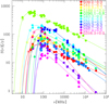 |
Fig. 1 Radio flux density measurements (coloured filled circles) as a function of frequency for 12 SNRs spectra with turnovers (see labels). This sample is built of 9 SNR spectra reported in Castelletti et al. (2021) plus 3 new spectra for the SNRs G189.1+3.0, G290.1–0.8, and G316.3+0.0, which were specifically constructed for this work. The solid coloured lines shows each corresponding best fit given by Eq. (2) with parameters included in our Table A.1. The asterisk symbol indicates the individual characteristic frequency, v* |
3 Analysis
SNRs that exhibit thermal turnovers are typically characterised by fitting the integrated continuum flux density S(v) at a frequency v using a power-law plus exponential cutoff equation:
![Mathematical equation: $S(v) = {S_0}{\left( {{v \over {{v_0}}}} \right)^\alpha }\exp \left[ { - {\tau _0}{{\left( {{v \over {{v_0}}}} \right)}^{ - 2.1}}} \right]$](/articles/aa/full_html/2024/04/aa46896-23/aa46896-23-eq1.png) (1)
(1)
where α is the power-law spectral index, S0 is a flux density normalisation, and τ0 is the free-free optical depth, both measured at a reference frequency, v0. The power-law term in this equation reflects the intrinsic synchrotron emission of the SNR, while the exponential term accounts for absorption due to ionised gas along the line of sight. However, because authors adopt different reference frequencies, typically related to their specific observing frequencies, it is often necessary to apply the scaling:  , where primed variables correspond to a reference frequency of
  . Some authors (e.g. Castelletti et al. 2021) use the same reference frequency (v0 = 74 MHz) for both physical process, namely, in the power law and in the exponential; others (e.g. Kassim 1989) presented their data using two different reference frequencies: one for the emission, v0 = 408 MHz, and one for the absorption, v0 = 30.9 MHz. Moreover, others (e.g. Kovalenko et al. 1994b) have used a unique reference frequency for absorption v0 = 100 MHz, but different ones for each individual SNR emission over a broad range from v0 = 175 MHz to v0 = 6000 MHz (see Table A.1). Although it is straightforward to convert values from one frequency to the other, the discordant parameterisation can make comparisons difficult. To avoid such complications, we can re-write Eq. (1) independent of the reference frequency as:
![Mathematical equation: $S(v) = {S_*}{\left( {{v \over {{v_*}}}} \right)^\alpha }\exp \left[ { - {{\left( {{v \over {{v_*}}}} \right)}^{ - 2.1}}} \right]$](/articles/aa/full_html/2024/04/aa46896-23/aa46896-23-eq4.png) (2)
(2)
where v* is a characteristic frequency and S* is a characteristic flux density. Equation (2) is identical to Eq. (1) but expressed by removing the explicit dependency of v0, τ0, and S0, that is, independently of the adopted reference frequency, v0. We notice that  and S* = S0(v*/v0)α. Computing these characteristic parameters using any other reference frequency gives the same values of v* and S*. Moreover, the physical meaning of these two parameters is straightforward: v* is related to the position of the turnover frequency vto, namely, where S(v) has its maximum, and S* is the spectrum normalisation height. The turnover frequency can be computed by deriving the flux density and equalising it to zero to yield vto/v* = (−2.1/α)1/2.1. Then, the characteristic frequency, v* is determined by both the turnover frequency, vto, and the power-law slope, α. It is only in the critical case where α = −2.1 that we have v* = vto, while for α > (<) − 2.1, we have v* < (>)vto. For a fiducial value of α ∼ −0.5, we obtain v* ~ vto/2, while for typical values of SNRs power-law slopes −0.89 ≲ α ≲ −0.35 (see Table A.1) we have 1.5 ≲ νto/ν. ≲ 2.5. It is worth noting that while Eq. (1) has been widely adopted by many authors, to the best of our knowledge, the simple parameterisation given by Eq. (2) has not been proposed before. An additional advantage of this parameterisation in terms of ν* is that low values of ν* indicate low νto or lower frequency turnovers, while high ν* values indicate high νto, with absorption commencing at higher frequencies.
To illustrate our approach to constrain the properties of the absorbing gas, in the next two subsections we apply these ideas to a sample of spectra for 129 SNRs, with and without observed turnovers. For the latter group, we utilise upper limits for ν. based on the lowest frequency measured.
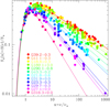 |
Fig. 2 Normalised radio flux density Sn(x) = S(v)/S, = xαexp(−x−2.1) measurements (coloured filled circles) as a function of the normalised frequency x = v/v* for 12 SNRs spectra with turnover (see labels). This sample comprises 9 SNR spectra reported in Castelletti et al. (2021), with the addition of three new spectra for the SNRs G189.1+3.0, G290.1–0.8, and G316.3+0.0 included for this work. Solid lines show their corresponding fit with parameters presented in our Table A.1. This normalised form sorts SNRs spectra in increasing order accordingly to their slope from bottom α = −0.89 to top α = −0.35. The black asterisk symbol marks the characteristic frequency v* and highlight how the normalisation has been done. |
3.1 SNRs with spectral turnovers
In Fig. 1, we display the measurements of 12 SNRs with turnovers, 9 of them reported by Castelletti et al. (2021), plus 3 more constructed for this work. Accordingly, Fig. 1 illustrates the complex superposition of spectra reflecting the relatively large range in spectral index (−0.89 ≲ α ≲ −0.35) and optical depth (0.016 ≲ τ0 ≲ 1.21 at ν0 = 74 MHz) listed in Table A.1.
In Fig. 2, we show the first advantage of the new parame-terisation offered through Eq. (2). Here, we plot the normalised flux density Sn(x) = S (ν)/S* as a function of the normalised frequency x = ν/ν* for the same 12 SNRs plotted in Fig. 1. The dynamic range of ~ 700 in S (ν) seen in Fig. 1 is reduced by at least a factor ~ 10 using the normalised form also showing a significantly smaller scatter. Moreover, the observational data at low frequencies, that is, lower than the characteristic frequency ν < ν* of the 12 SNRs when stacked together, are well fit by a unique drop-off curve A(x) = exp(−x−2.1) that is more clearly traced than in the individual curves. At high frequencies, namely, those that are higher than the characteristic frequency ν > ν*, the solid curves differ only due to their slopes α. Power-law emissions are ordered by their slope from a steep α = −0.89 value for G316.3+0.0 (bright pink filled circles and solid curve) to a flat α = −0.35 for G39.2−0.3 (red filled circles and solid curve).
In Fig. 3, we applied an additional normalisation step by dividing the flux density Sn(x) by the power-law emission factor of each SNR, E(x) = xα. Another advantage of the new normalisation is that any SNR spectrum can be fit by a unique absorption equation A(x) = exp(−x−2.1), as depicted by the solid black curve. A reduced rms scatter of ~11% is apparent for these 12 SNRs stacked together indicating the quality of the fits. To enlarge our sample, we also compiled spectra with a low-frequency turnover of 14 SNRs reported in Kassim (1989) and 31 from Kovalenko et al. (1994b). These dataset are represented by filled small black squares and triangles, respectively. The inclusion of these two additional samples reinforces our results showing a similar trend, albeit with a higher rms scatter.
3.2 Pure power-law SNRs spectra
Pure power-law spectra can be interpreted as absorbed spectra as well, but absorbed at such low frequencies that the turnover has not been observationally detected yet. For example, if the turnover frequency is at ν* = 30 MHz, but there are no quality measurements at comparable frequencies, the spectrum is usually fit by a pure power-law. Indeed, if a turnover has not been detected, the lowest measured frequency, νlow, of a spectrum can be considered as an upper limit for the undetected turnover frequency. We therefore expanded our sample of turnover spectra by assigning a turnover to the pure power law fits, allowing for a maximum of a 10% difference between the extrapolated power law and the absorbed fit at the lowest frequency. Using Eq. (2), we have ν* = νlow(loge ƒ)1/2.1 where ƒ is a parameter that fixes the ratio between the flux density power law and the turnover fit at νlow. We have adopted a value of ƒ = 1.1, which means that the difference is 10% yielding ν* ~ 0.33νlow.
Figures 4, 5, and 6 are analogous to Figs. 1, 2, and 3, respectively, but constructed for SNRs whose integrated radio continuum spectra are fitted by pure power laws. Two of the plotted spectra are taken from Castelletti et al. (2021) and the other 15 were constructed for the purposes of this work, as explained in Sect. 2. In Fig. 4, the coloured solid lines are the corresponding pure power-law best fits to the data points of each SNR, while the dotted lines are the putative turnover spectra given by Eq. (2). The asterisk symbols indicate the maximum characteristic frequency ν. allowed by the lowest frequency observed νlow. Again, the large dynamic range in measured flux densities of ~300 is reduced by a factor of ~7 when the normalised form is adopted (see Fig. 5). A final normalisation to the individual power law slope α shows good quality fits with rms of ~15% as seen in the coloured open circles of Fig. 6. These fits are better quality than the pure power-law samples of Kovalenko et al. (1994b) and Kassim (1989) depicted by open small black squares and triangles, respectively.
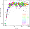 |
Fig. 3 Normalised radio flux density measurement as a function of frequency for 9 SNR spectra presented in Castelletti et al. (2021) plus 3 new spectra for the SNRs G189.1+3.0, G290.1−0.8, and G316.3+0.0, constructed for this work (coloured filled circles), along with data from Kovalenko et al. (1994b) (black filled squares) and Kassim (1989) (black filled triangles). In order to highlight the drop-off behavior, the data are normalised to the power-law emission E(x) = xα, where x = ν/ν*. The curved solid line is the normalised absorption A(x) = exp(−x−2.1). The total root mean square (rms) of the coloured circles is less than 11%. At ν ~ 2.75ν, approximately 50% of the emission is absorbed. |
3.3 Characteristic frequency ν* distribution
In Fig. 7, we show as a filled histogram the distribution of ν. values, computed for our three samples (Castelletti et al. 2021 plus this work, Kovalenko et al. 1994b, and Kassim 1989 listed in Table A.1) ranging from ~10 MHz to 100 MHz. In the upper panel, v* ~ 40 MHz separates two populations with low (τ ~ 0.1) and high (τ ~ 1) optical depths reported in Table 3 of Castelletti et al. (2021); these two subsam-ples were labeled as ‘Absorption from extended envelopes’ (non-local) and ‘Absorption: Special cases’ (local), respectively. The classification was made by additional information obtained from low-frequency radio recombination lines, infrared fine-structure, and molecular line emission to distinguish between spectral turnovers attributed to ionised material in the ISM unrelated to the SNR (non-local) and an ionised component in the SNR’s immediate surroundings (local). These low (v* ≲ 40 MHz) and high (v* ≳ 40 MHz) populations might hint at nonlocal vs. local absorbers in the other two samples, Kassim (1989) and Kovalenko et al. (1994b), shown in the middle and bottom panels of Fig. 7. However, due to the incompleteness of our samples, it is not possible to definitively determine yet whether these populations represent truly distinct groups or merely the low and high tails of a single population with intrinsic dispersion. The open histograms show the characteristic frequency v* of power-law spectra assigned according to their observed lowest frequency, vlow. In the upper panel, the observed peak at v* ~ 30 MHz is a direct consequence of the GLEAM survey cutoff frequency at vlow ~ 88 MHz (see asterisk symbols in Fig. 4). At v* ~ 10 MHz we have measurements obtained at lower frequencies by the Clark Lake TPT (30.9 MHz), Culgoora (80 MHz), and Pushchino (83 MHz) telescopes (see Sect. 2).
We notice that the upper colour bar indicates the colour coding adopted in Figs. 8 and 9 based on log(v*/MHz) value instead of using the SNRs’ names, as done in Figs. 1–6, as well as in Figs. 10 and 11. On the other hand, we also searched for (but did not find) any significant correlations between the three fitted parameters S*, v* and α. This result indicates that the emission and absorption processes in our limited SNR sample are independent of each other. A useful and direct application of the characteristic frequency, v* parameterisation is the possibility to provide insights concerning the properties of the absorbing thermal gas. A complete mapping of the v* distribution in the Galaxy should offer strong and unique constraints on the distribution of the ionised absorbing gas. Despite the incomplete and non-uniform nature of current surveys on SNRs, we utilised our compiled sample to extract fundamental and widespread characteristics from the presently available data. Additionally, we have compared our findings with ad-hoc constructed models in order to draw initial conclusions regarding the absorber population. In Fig. 8, we show the projected spatial distribution onto the Galactic plane for all the SNRs with turnovers (filled symbols) in our three samples. We have also included SNRs from Castelletti et al. (2021) plus this work, Kovalenko et al. (1994b), and Kassim (1989), whose spectra are well fitted by a pure power law (open symbols) coloured according to the upper limit of the characteristic frequency assigned to them (see Sect. 3.2 and Fig. 4). At first glance, it does not appear that there is a significant segregation between SNRs with and without spectral turnovers, or an apparent gradient in v* with global properties like heliocentric distance or Galactic longitude. This qualitative result indicates that the absorbing media is probably made of discrete ionised regions rather than a continuous gas distribution. Likewise, the absence of spectral turnover in some distant SNRs, coupled with significant absorption in some nearby ones, was first interpreted by Kassim (1989) as a patchy distribution of low-frequency absorbing gas, and not caused by a broadly distributed component of the ISM. Here, we test this original idea by adding the spectra presented by Castelletti et al. (2021), those constructed for this work, along with those included in Kovalenko et al. (1994b).
To facilitate the interpretation of these observational findings, in the following section, we describe how we developed a two-dimensional (2D) toy model that simulates the power-law emission from SNRs and takes into account the absorption caused by intervening ionising gas.
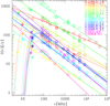 |
Fig. 4 Radio flux density measurements (coloured open circles) as a function of frequency for 17 SNRs spectra without turnovers (see labels). This sample includes the spectra of SNRs G4.5+6.8 and G28.6-0.1 published in Castelletti et al. (2021) plus 15 new ones constructed for this work. The solid coloured lines shows each corresponding power-law best fit, while the dotted ones correspond to Eq. (2) with a characteristic frequency v, (see asterisk symbol) assigned as an upper limit according to the lowest measured frequency, vlow. |
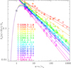 |
Fig. 5 Normalised radio flux density Sn(x) = S(v)/S, = xαexp(−x−21) measurements (coloured open circles) as a function of the normalised frequency x = v/v* for 17 SNRs spectra without low frequency turnover (see labels). This sample includes the spectra of G4.5+6.8 and G28.6-0.1 SNRs published in Castelletti et al. (2021), plus 15 new collected for this work. Extended lines show their power-law fit while dotted ones correspond to Eq. (2) with characteristic frequency, v* (asterisk symbol) assigned as an upper limit according to the lowest measured frequency vlow. This normalised form sorts SNRs spectra in increasing order accordingly to their slope from bottom α = −0.69 to top α = −0.32. The black asterisk symbol marks the characteristic frequency, v*, and highlights how the normalisation is done. |
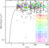 |
Fig. 6 Normalised radio flux density measurements as a function of frequency for the SNRs G4.5+6.8 and G28.6–0.1 presented in Castelletti et al. (2021) plus 15 new SNR spectra constructed for this work (coloured open circles). These datasets are complemented by flux density estimates from Kovalenko et al. (1994b) as black open squares and Kassim (1989) as black open triangles. In order to highlight the drop-off behavior, the data are normalised to the power-law emission E(x) = xα, where x = v/v*. The curved solid line is the normalised absorption A(x) = exp(−x−2.1). The total rms of the coloured open circles is less than 15%. |
4 Absorption model
We assumed that the SNRs are distributed on the Galactic plane following an exponential surface number density profile: Σ(R) = Σ0 exp(−R/Rd), where Σ0 is the central surface density and Rd is the scale-length. We tied Σ0 to a mock assumption of 20 000 SNRs sufficiently large to mimic the statistical behavior of a generic population of remnants distributed on the Galactic plane with Rd = 3.5 kpc following the Milky Way stellar scale-length. We started by attributing the absorption to ionised gas characterised by an emission measure (see Eq. (6) and discussion below) predicted by the continuum model NE2001, at a fixed temperature (Cordes & Lazio 2002). We found that the NE2001 model predicts a correlation between absorption and distance, a correlation that is not observed. We attribute the discrepancy to the fact that the NE2001 model assumes a nearly continuous distribution of ionised gas, together with its reliance on measurements of relatively nearby pulsars (PSRs). Recognising that H II regions are discrete structures, we then considered a model in which a set of discrete absorbing regions, representing H II regions or H II region complexes, are distributed throughout the disk of the Galaxy.
We place clumps of ionised gas preferentially along the Galactic spiral arms following the Hou & Han (2014) four-arm logarithmic model (see their Table 1). Clumps are circular with radius, r, drawn from a Maxwell-Boltzmann probability density distribution:
 (3)
(3)
with a parameter a = 50 pc. Initially, we distribute homogeneously clumps along the spiral arms; then we add a random noise of 5% in their polar radius to mimic the fact that H II regions are not perfectly distributed along the spiral arms and also that the spiral arms themselves are not perfectly delineated in real galaxies. We also fixed the number of absorbers in a way so that the initial (i.e. before adding the random noise) mean separation between them is five times their typical size. Altogether, these conditions result in 981 simulated H II regions that trace approximately the spiral arms and that they do not overlap. This is consistent with the number and distribution of Galactic H II regions revealed by observational surveys that typically point out hundreds to thousands of these objects (Anderson et al. 2018; Wenger et al. 2021, and references therein).
The predicted characteristic frequency, v* can be estimated using its definition, introduced in Sect. 3,  , where the optical depth, τ0, can be computed from the physical properties of the absorbing ionised gas using the following equation (Wilson et al. 2009):
 (4)
(4)
where Te is the gas electron temperature,
![Mathematical equation: ${{\rm{g}}_{{\rm{ff}}}} = {\log _e}\left[ {4.955 \times {{10}^{ - 2}}{{\left( {{{{v_0}} \over {{\rm{GHz}}}}} \right)}^{ - 1}}} \right] + 1.5{\log _e}\left( {{{{{\rm{T}}_{\rm{e}}}} \over {\rm{K}}}} \right)$](/articles/aa/full_html/2024/04/aa46896-23/aa46896-23-eq9.png) (5)
(5)
is the Gaunt factor, and
 (6)
(6)
is the emission measure depending on the electron density, ne, integrated along the linear length, L, of the intervening medium. Assuming a constant electron density, the emission measure is  . Therefore, we have
  , namely, the characteristic frequency depends more strongly on the electron density adopted, less on the electron temperature, and more weakly on the path L. We assume constant electron temperature Te = 5000 K and density ne = 2.0 cm−3 (Castelletti et al. 2021).
By adopting these values, our model is calibrated to reproduce an average value v* ~30 MHz observed in the combined sample of Castelletti et al. (2021) plus this work, Kovalenko et al. (1994b), and Kassim (1989) (see Fig. 7). The linear length, L, is computed as the cumulative sum of all segments along the integral that intersect circular ionised clumps of radius, r, along the line of sight from the solar position. We notice that the NE2001 model cannot predict such characteristic frequencies v* ~ 30 MHz for SNRs that are located nearby (i.e. at heliocentric distances of ~ 1 kpc) due to the low electron density assumed (ne ~ 0.2 cm−3), which is approximately one order of magnitude lower than that inferred from the SNR turnover spectra by Castelletti et al. (2021).
The prediction of our model is shown in Fig. 9, where the spatial distribution of the emitters (SNRs) are plotted as coloured dots (using the colour coding shown in the upper bar), while the absorbers are displayed as black open circles. To make the plot more clear the scale of each open circle has been expanded by an arbitrary factor of 3. The observer is assumed to be at Cartesian coordinates (0,8.5) kpc from the Galactic centre mimicking the Sun’s position. The coloured points correspond to SNRs that are absorbed by ionised gas along the line of sights. In a model of sparse and discrete absorbers, as this one, SNRs with and without spectral turnover are predicted to be mixed, namely, not spatially segregated as expected in a model with absorbers continuously distributed. In a continuous model, SNRs with nonthermal turnovers are expected to be located closer to the observer while those showing turnovers should exhibit characteristic frequencies, v* increasing with distance. This is because the radiation passes through more gas as it travels towards the observer, leading to increased intersection and thus a higher predicted frequency. We notice that the asymmetric coil of spiral arms, namely, that its Galacto-centric distance increases with its polar angle, makes absorption asymmetric between the first and fourth and between the second and third quadrants. The strongest absorption is predicted in the fourth quadrant tangential direction (see magenta dots) of the most internal spiral arm.
We conducted a series of tests on our model using different values of the scale-length parameter, Rd, for the exponential distribution of SNRs. We also experimented with using a power-law profile, Σ(R) = Σ0(R/Rd)γ. Despite these changes, we found that our results remained consistent and robust.
To compare the observational results against the predictions of our simple model, in Figs. 10 and 11 we plot the characteristic frequency, v* as a function of the heliocentric distance and the Galactic longitude, respectively. Observational values for spectra with turnovers, indicated by coloured filled circles (Castelletti et al. 2021 plus this work), small black filled squares (Kovalenko et al. 1994b) and small black filled triangles (Kassim 1989), show neither a positive gradient with distance nor a negative gradient with Galactic longitude, as expected in a model of continuously distributed absorbing gas. Theoretical models featuring discrete absorbers (as depicted in Fig. 9) reveal that the values of v* remain approximately constant. This indicates that absorption is independent of heliocentric distance or Galactic longitude, as illustrated by the black continuous solid line. Besides, we have also included observed SNRs with no measured spectral turnovers (i.e. sources with pure power-law continuum spectra) with v* computed as the upper limit allowed by the lowest observed frequency vlow (see Sect. 3.2). These remnants are located not only quite close, d ~ 2 kpc, to the solar position, but also at distances as large as d ~ 10 kpc. Similarly, they can be found either quite close the Galactic centre or in the anticentre direction.
Based on our assumed distribution of H II regions following the spiral arms, we find that the absorption of our mock SNR population is consistent with the patchy distribution of absorption indicated by observations to date. A much larger sample of low frequency spectra are needed to verify if our model of absorbing gas due to H II regions is the correct approach.
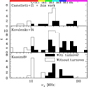 |
Fig. 7 Histograms showing the distribution of characteristic frequencies, v* for the three samples analyzed here. Each panel corresponds to a different sample, as indicated by the labels. The filled histograms show the distribution of v* for SNRs spectra with turnovers, while the open ones depict the estimated upper limit of v* based on the lowest measured frequency, vlow, for spectra without turnovers. |
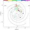 |
Fig. 8 Projected spatial distribution onto the Galactic plane of SNRs in the three samples analyzed here with distances taken from Ranasinghe & Leahy (2022) and coloured according to log(ν∗/MHz) using the colour bar code. Filled symbols show the location of SNRs with turnover spectra, while the open symbols indicate those sources not showing turnovers. Circles correspond to Castelletti et al. (2021) plus this work data, squares correspond to Kovalenko et al. (1994b), and triangles to Kassim (1989). As a guidance the solid black lines show the position of the spiral arms taken from the Hou & Han (2014) model. The central plus symbol indicates the position of the Galactic centre, the solar symbol shows the Sun’s position, and the dotted lines the Galactic quadrants. The coloured points do not show any strong dependence on heliocentric distance or Galactic longitude (see Figs. 10 and 11). |
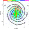 |
Fig. 9 Spatial distribution of an assumed mock sample of 20 000 SNRs (points coloured by log(v*/MHz) using the colour bar code). Absorbers (open circles) are distributed along the Galactic spiral arms taken from the Hou & Han (2014) model (solid black curves). Each absorber is assumed to have a constant low density ne = 2.0 cm−3, a temperature Te = 5000 K, and radius r drawn from a Maxwell-Boltzmann probability density distribution with a median of 50 pc. The scale of each open circle has been expanded by an arbitrary factor of 3 in order to make the plot clearer. The central plus symbol indicates the position of the Galactic centre, the solar symbol shows the Sun’s position, and the dotted lines the Galactic quadrants. The coloured points do not show any strong dependence on heliocentric distance or Galactic longitude (see Figs. 10 and 11). |
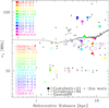 |
Fig. 10 Characteristic frequency, v*, as a function of the heliocentric distance for SNRs with low frequency turnovers (filled symbols) and SNRs spectra without turnovers (open symbols). Circles correspond to Castelletti et al. (2021) plus this work data, while squares to Kovalenko et al. (1994b), and triangles to Kassim (1989). The solid line corresponds to the median prediction of the model presented in Fig. 9 not showing a systematic gradient with heliocentric distance. |
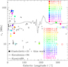 |
Fig. 11 Characteristic frequency, v* as a function of the Galactic longitude for SNRs with low frequency turnovers (filled symbols) and SNRs spectra without turnovers (open symbols). Circles correspond to Castelletti et al. (2021) plus this work data, while squares to Kovalenko et al. (1994b), and triangles to Kassim (1989). The solid line corresponds to the median prediction of the model presented in Fig. 9, which does not show a strong dependence with the Galactic longitude. |
5 Conclusions
We have analyzed a sample of 129 radio continuum spectra of Galactic SNRs from this work and the literature (including Castelletti et al. 2021; Kovalenko et al. 1994b; and Kassim 1989). Among them, 57 show low-frequency turnovers characteristic of extrinsic thermal absorption, while 72 remain straight power laws (special cases of intrinsic absorption by unshocked ejecta within SNRs is not considered in this paper). Since the frequencies sampled vary across the spectra, we take care to interpret the latter as limits on absorption in context of their lowest frequency measurement. Our main conclusions are:
We introduced a new parameterisation of the SNR integrated radio-continuum spectra in terms of characteristic frequency, v*, and corresponding flux density, S*, independent of arbitrary survey reference frequencies. Here, v* is directly related both to the power-law emission slope and the turnover frequency, including the density, temperature, and path through the absorbing medium;
By normalising the SNR spectra to the frequency, v*, and to the flux density, S*, we confirmed, with our larger sample, that while all SNRs emit energy with independent synchrotron emission power-law indices, turnovers are all well fit by thermal absorption;
For SNRs not showing turnovers, we derived an upper limit for v* by considering the lowest sampled frequency yielding a range of 4 MHz ≲ v* ≲ 40 MHz. This result should be tested and improved by forthcoming surveys pushing SNR spectra to lower frequencies, especially <50 MHz where sensitivity to absorption is markedly increased;
Emission (α) and absorption (v*) spectral parameters do not show any significant correlation indicating two unrelated, independent processes. For example, absorption beyond the nominal boundaries of the synchrotron emitting plasma seem oblivious to the details and history of the shock acceleration processes within the remnant. For our three samples of SNR spectra with turnovers we found the characteristic frequency ranges of 10 MHz ≲ v* ≲ 100 MHz;
There is no evidence for a correlation between absorption and global Galactic geometric parameters such as heliocentric distance and Galactic longitude, as would be expected if the distribution of the absorbing gas were continuous. Our result is also valid for pure power-law SNR spectra. This is consistent with Kassim (1989) who inferred that SNRs were being absorbed by an intervening patchy distribution of H II regions or their envelopes whose distances were unknown;
Modelling based on a distribution of H II regions tracking Galactic spiral arms produces patchy absorption towards a mock SNR population consistent with the limited observations to date. One prediction of this scheme is that strongly absorbed SNRs should be located preferentially towards the fourth Galactic quadrant relative to the first;
Emission measures predicted from NE2001 could not match the observations. We attribute the discrepancy to the fact that the NE2001 model assumes a nearly continuous distribution of ionised gas and relies predominantly on a relatively nearby population of PSRs. The NE2001 model predicts a correlation between absorption and distance, particularly for greater distances, that is not observed.
Unfortunately, the incompleteness of current SNR catalogs, and absence of low frequency spectra, even for those that are known, preclude making a much more detailed comparison between models and observations. This motivates the completion of deeper, global surveys at both MHz and GHz frequencies to push all SNR spectra to lower frequencies and to fully sample the intrinsic properties such as density, temperature, size, and distance, of intervening Galactic thermal gas. Arc-second resolution observations below 100 MHz, as provided by LOFAR and emerging low-frequency instruments such as LWA and Square Kilometre Array-Low, are critical for discerning the relative radial superposition of SNRs and H II regions along complex lines of sight. Given readily available kinematic distances to H II regions, this can offer powerful physical constraints for SNRs whose distances are far more problematic.
Acknowledgements
This work has been partially supported by the Consejo de Investigaciones Científicas y Técnicas de la República Argentina (CONICET), the Secretaría de Ciencia y Técnica de la Universidad Nacional de Córdoba (SeCyT), Agencia Nacional de Promoción Científica y Tecnológica (PICT 20173320, PICT 2019-1600), Argentina. M.A. acknowledges the hospitality of the Astronomical Observatory of Trieste where part of the work was done in the framework of the European Union LACEGAL program. Basic research in radio astronomy at the Naval Research Laboratory is funded by 6.1 Base funding. Part of this research was carried out at the Jet Propulsion Laboratory, California Institute of Technology, under a contract with the National Aeronautics and Space Administration.
Appendix A SNR radio-continuum spectral parameters
Radio continuum spectral parameters for the SNR sample used in this work.
References
- Anantharamaiah, K. R. 1985, J. Astrophys. Astron., 6, 203 [NASA ADS] [CrossRef] [Google Scholar]
- Anderson, L. D., Armentrout, W. P., Luisi, M., et al. 2018, ApJS, 234, 33 [NASA ADS] [CrossRef] [Google Scholar]
- Arias, M., Vink, J., de Gasperin, F., et al. 2018, A&A, 612, A110 [NASA ADS] [CrossRef] [EDP Sciences] [Google Scholar]
- Arias, M., Vink, J., Zhou, P., et al. 2019, AJ, 158, 253 [NASA ADS] [CrossRef] [Google Scholar]
- Bietenholz, M. F., Kassim, N., Frail, D. A., et al. 1997, ApJ, 490, 291 [NASA ADS] [CrossRef] [Google Scholar]
- Blandford, R., & Eichler, D. 1987, Phys. Rep., 154, 1 [Google Scholar]
- Braude, S. Y., Lebedeva, O. M., Megn, A. V., Ryabov, B. P., & Zhouck, I. N. 1969, MNRAS, 143, 289 [NASA ADS] [Google Scholar]
- Braude, S. I., Megn, A. V., Sokolov, K. P., Tkachenko, A. P., & Sharykin, N. K. 1979, Ap&SS, 64, 73 [NASA ADS] [CrossRef] [Google Scholar]
- Bridle, A. H., & Purton, C. R. 1968, AJ, 73, 717 [NASA ADS] [CrossRef] [Google Scholar]
- Brogan, C. L., Lazio, T. J., Kassim, N. E., & Dyer, K. K. 2005, AJ, 130, 148 [NASA ADS] [CrossRef] [Google Scholar]
- Carretti, E., Haverkorn, M., Staveley-Smith, L., et al. 2019, MNRAS, 489, 2330 [Google Scholar]
- Castelletti, G., Supan, L., Peters, W. M., & Kassim, N. E. 2021, A&A, 653, A62 [NASA ADS] [CrossRef] [EDP Sciences] [Google Scholar]
- Cordes, J. M., & Lazio, T. J. W. 2002, arXiv e-prints [arXiv:0207156] [Google Scholar]
- DeLaney, T., Kassim, N. E., Rudnick, L., & Perley, R. A. 2014, ApJ, 785, 7 [NASA ADS] [CrossRef] [Google Scholar]
- Dulk, G. A., & Slee, O. B. 1972, Aust. J. Phys., 25, 429 [NASA ADS] [CrossRef] [Google Scholar]
- Dulk, G. A., & Slee, O. B. 1975, ApJ, 199, 61 [CrossRef] [Google Scholar]
- Erickson, W. C., & Cronyn, W. M. 1965, ApJ, 142, 1156 [NASA ADS] [CrossRef] [Google Scholar]
- Haynes, R. F., Caswell, J. L., & Simons, L. W. J. 1978, Aust. J. Phys. Astrophys. Suppl., 45, 1 [NASA ADS] [Google Scholar]
- Hou, L. G., & Han, J. L. 2014, A&A, 569, A125 [NASA ADS] [CrossRef] [EDP Sciences] [Google Scholar]
- Hurley-Walker, N., Hancock, P. J., Franzen, T. M. O., et al. 2019, PASA, 36, e047 [Google Scholar]
- Jones, B. B., & Finlay, E. A. 1974, Aust. J. Phys., 27, 687 [NASA ADS] [CrossRef] [Google Scholar]
- Kassim, N. E. 1988, ApJS, 68, 715 [NASA ADS] [CrossRef] [Google Scholar]
- Kassim, N. E. 1989, ApJ, 347, 915 [NASA ADS] [CrossRef] [Google Scholar]
- Kassim, N. E., Perley, R. A., Dwarakanath, K. S., & Erickson, W. C. 1995, ApJ, 455, L59 [NASA ADS] [CrossRef] [Google Scholar]
- Kovalenko, A. V., Pynzar’, A. V., & Udal’Tsov, V. A. 1994a, AZh, 71, 110 [NASA ADS] [Google Scholar]
- Kovalenko, A. V., Pynzar’, A. V., & Udal’Tsov, V. A. 1994b, Astron. Rep., 38, 78 [NASA ADS] [Google Scholar]
- Lacey, C. K., Lazio, T. J. W., Kassim, N. E., et al. 2001, ApJ, 559, 954 [NASA ADS] [CrossRef] [Google Scholar]
- Lane, W. M., Clarke, T. E., Taylor, G. B., Perley, R. A., & Kassim, N. E. 2004, AJ, 127, 48 [NASA ADS] [CrossRef] [Google Scholar]
- Malkov, M. A., & Drury, L. O. 2001, Rep. Progr. Phys., 64, 429 [Google Scholar]
- McClure-Griffiths, N. M., Dickey, J. M., Gaensler, B. M., et al. 2005, ApJS, 158, 178 [NASA ADS] [CrossRef] [Google Scholar]
- Mills, B. Y., & Slee, O. B. 1957, Aust. J. Phys., 10, 162 [NASA ADS] [CrossRef] [Google Scholar]
- Mills, B. Y., Slee, O. B., & Hill, E. R. 1958, Aust. J. Phys., 11, 360 [NASA ADS] [CrossRef] [Google Scholar]
- Mills, B. Y., Slee, O. B., & Hill, E. R. 1960, Aust. J. Phys., 13, 676 [NASA ADS] [CrossRef] [Google Scholar]
- Ranasinghe, S., & Leahy, D. 2022, ApJ, 940, 63 [NASA ADS] [CrossRef] [Google Scholar]
- Rishbeth, H. 1958, Aust. J. Phys., 11, 550 [NASA ADS] [CrossRef] [Google Scholar]
- Roger, R. S., Costain, C. H., & Lacey, J. D. 1969, AJ, 74, 366 [NASA ADS] [CrossRef] [Google Scholar]
- Roger, R. S., Costain, C. H., & Stewart, D. I. 1986, A&AS, 65, 485 [NASA ADS] [Google Scholar]
- Slee, O. B. 1977, Aust. J. Phys. Astrophys. Suppl., 43, 1 [NASA ADS] [Google Scholar]
- Slee, O. B., & Higgins, C. S. 1973, Aust. J. Phys. Astrophys. Suppl., 27, 1 [NASA ADS] [Google Scholar]
- Slee, O. B., & Higgins, C. S. 1975, Aust. J. Phys. Astrophys. Suppl., 36, 1 [NASA ADS] [Google Scholar]
- Viner, M. R., & Erickson, W. C. 1975, AJ, 80, 931 [NASA ADS] [CrossRef] [Google Scholar]
- Wenger, T. V., Dawson, J. R., Dickey, J. M., et al. 2021, ApJS, 254, 36 [NASA ADS] [CrossRef] [Google Scholar]
- Williams, P. J. S., Kenderdine, S., & Baldwin, J. E. 1966, MmRAS, 70, 53 [NASA ADS] [Google Scholar]
- Wilson, T. L., Rohlfs, K., & Hüttemeister, S. 2009, Tools of Radio Astronomy (Berlin: Springer/Berlin Heidelberg) [Google Scholar]
Additional flux density measurements below 100 MHz, which were included in our spectral analysis and obtained from the literature, are as follows: 10 MHz (Bridle & Purton 1968), 19 MHz (Rishbeth 1958), 1025 MHz (Braude et al. 1969, 1979), 22 MHz (Roger et al. 1969, 1986), 26 MHz (Erickson & Cronyn 1965; Viner & Erickson 1975), 29.9 MHz (Jones & Finlay 1974), 38 MHz (Williams et al. 1966), and 86 MHz (Mills & Slee 1957; Mills et al. 1958, 1960).
All Tables
All Figures
|
Fig. 1 Radio flux density measurements (coloured filled circles) as a function of frequency for 12 SNRs spectra with turnovers (see labels). This sample is built of 9 SNR spectra reported in Castelletti et al. (2021) plus 3 new spectra for the SNRs G189.1+3.0, G290.1–0.8, and G316.3+0.0, which were specifically constructed for this work. The solid coloured lines shows each corresponding best fit given by Eq. (2) with parameters included in our Table A.1. The asterisk symbol indicates the individual characteristic frequency, v* |
| In the text | |
|
Fig. 2 Normalised radio flux density Sn(x) = S(v)/S, = xαexp(−x−2.1) measurements (coloured filled circles) as a function of the normalised frequency x = v/v* for 12 SNRs spectra with turnover (see labels). This sample comprises 9 SNR spectra reported in Castelletti et al. (2021), with the addition of three new spectra for the SNRs G189.1+3.0, G290.1–0.8, and G316.3+0.0 included for this work. Solid lines show their corresponding fit with parameters presented in our Table A.1. This normalised form sorts SNRs spectra in increasing order accordingly to their slope from bottom α = −0.89 to top α = −0.35. The black asterisk symbol marks the characteristic frequency v* and highlight how the normalisation has been done. |
| In the text | |
|
Fig. 3 Normalised radio flux density measurement as a function of frequency for 9 SNR spectra presented in Castelletti et al. (2021) plus 3 new spectra for the SNRs G189.1+3.0, G290.1−0.8, and G316.3+0.0, constructed for this work (coloured filled circles), along with data from Kovalenko et al. (1994b) (black filled squares) and Kassim (1989) (black filled triangles). In order to highlight the drop-off behavior, the data are normalised to the power-law emission E(x) = xα, where x = ν/ν*. The curved solid line is the normalised absorption A(x) = exp(−x−2.1). The total root mean square (rms) of the coloured circles is less than 11%. At ν ~ 2.75ν, approximately 50% of the emission is absorbed. |
| In the text | |
|
Fig. 4 Radio flux density measurements (coloured open circles) as a function of frequency for 17 SNRs spectra without turnovers (see labels). This sample includes the spectra of SNRs G4.5+6.8 and G28.6-0.1 published in Castelletti et al. (2021) plus 15 new ones constructed for this work. The solid coloured lines shows each corresponding power-law best fit, while the dotted ones correspond to Eq. (2) with a characteristic frequency v, (see asterisk symbol) assigned as an upper limit according to the lowest measured frequency, vlow. |
| In the text | |
|
Fig. 5 Normalised radio flux density Sn(x) = S(v)/S, = xαexp(−x−21) measurements (coloured open circles) as a function of the normalised frequency x = v/v* for 17 SNRs spectra without low frequency turnover (see labels). This sample includes the spectra of G4.5+6.8 and G28.6-0.1 SNRs published in Castelletti et al. (2021), plus 15 new collected for this work. Extended lines show their power-law fit while dotted ones correspond to Eq. (2) with characteristic frequency, v* (asterisk symbol) assigned as an upper limit according to the lowest measured frequency vlow. This normalised form sorts SNRs spectra in increasing order accordingly to their slope from bottom α = −0.69 to top α = −0.32. The black asterisk symbol marks the characteristic frequency, v*, and highlights how the normalisation is done. |
| In the text | |
|
Fig. 6 Normalised radio flux density measurements as a function of frequency for the SNRs G4.5+6.8 and G28.6–0.1 presented in Castelletti et al. (2021) plus 15 new SNR spectra constructed for this work (coloured open circles). These datasets are complemented by flux density estimates from Kovalenko et al. (1994b) as black open squares and Kassim (1989) as black open triangles. In order to highlight the drop-off behavior, the data are normalised to the power-law emission E(x) = xα, where x = v/v*. The curved solid line is the normalised absorption A(x) = exp(−x−2.1). The total rms of the coloured open circles is less than 15%. |
| In the text | |
|
Fig. 7 Histograms showing the distribution of characteristic frequencies, v* for the three samples analyzed here. Each panel corresponds to a different sample, as indicated by the labels. The filled histograms show the distribution of v* for SNRs spectra with turnovers, while the open ones depict the estimated upper limit of v* based on the lowest measured frequency, vlow, for spectra without turnovers. |
| In the text | |
|
Fig. 8 Projected spatial distribution onto the Galactic plane of SNRs in the three samples analyzed here with distances taken from Ranasinghe & Leahy (2022) and coloured according to log(ν∗/MHz) using the colour bar code. Filled symbols show the location of SNRs with turnover spectra, while the open symbols indicate those sources not showing turnovers. Circles correspond to Castelletti et al. (2021) plus this work data, squares correspond to Kovalenko et al. (1994b), and triangles to Kassim (1989). As a guidance the solid black lines show the position of the spiral arms taken from the Hou & Han (2014) model. The central plus symbol indicates the position of the Galactic centre, the solar symbol shows the Sun’s position, and the dotted lines the Galactic quadrants. The coloured points do not show any strong dependence on heliocentric distance or Galactic longitude (see Figs. 10 and 11). |
| In the text | |
|
Fig. 9 Spatial distribution of an assumed mock sample of 20 000 SNRs (points coloured by log(v*/MHz) using the colour bar code). Absorbers (open circles) are distributed along the Galactic spiral arms taken from the Hou & Han (2014) model (solid black curves). Each absorber is assumed to have a constant low density ne = 2.0 cm−3, a temperature Te = 5000 K, and radius r drawn from a Maxwell-Boltzmann probability density distribution with a median of 50 pc. The scale of each open circle has been expanded by an arbitrary factor of 3 in order to make the plot clearer. The central plus symbol indicates the position of the Galactic centre, the solar symbol shows the Sun’s position, and the dotted lines the Galactic quadrants. The coloured points do not show any strong dependence on heliocentric distance or Galactic longitude (see Figs. 10 and 11). |
| In the text | |
|
Fig. 10 Characteristic frequency, v*, as a function of the heliocentric distance for SNRs with low frequency turnovers (filled symbols) and SNRs spectra without turnovers (open symbols). Circles correspond to Castelletti et al. (2021) plus this work data, while squares to Kovalenko et al. (1994b), and triangles to Kassim (1989). The solid line corresponds to the median prediction of the model presented in Fig. 9 not showing a systematic gradient with heliocentric distance. |
| In the text | |
|
Fig. 11 Characteristic frequency, v* as a function of the Galactic longitude for SNRs with low frequency turnovers (filled symbols) and SNRs spectra without turnovers (open symbols). Circles correspond to Castelletti et al. (2021) plus this work data, while squares to Kovalenko et al. (1994b), and triangles to Kassim (1989). The solid line corresponds to the median prediction of the model presented in Fig. 9, which does not show a strong dependence with the Galactic longitude. |
| In the text | |
Current usage metrics show cumulative count of Article Views (full-text article views including HTML views, PDF and ePub downloads, according to the available data) and Abstracts Views on Vision4Press platform.
Data correspond to usage on the plateform after 2015. The current usage metrics is available 48-96 hours after online publication and is updated daily on week days.
Initial download of the metrics may take a while.