| Issue |
A&A
Volume 684, April 2024
|
|
|---|---|---|
| Article Number | A53 | |
| Number of page(s) | 21 | |
| Section | Extragalactic astronomy | |
| DOI | https://doi.org/10.1051/0004-6361/202245754 | |
| Published online | 01 April 2024 | |
Constraints on the densities and temperature of the Seyfert 2 narrow line region
1
Instituto de Astronomía, Universidad Nacional Autónoma de México, Apdo. Postal 70-264, 04510 D.F., México, Mexico
e-mail: This email address is being protected from spambots. You need JavaScript enabled to view it.
2
Département de physique, de génie physique et d’optique, Université Laval, Québec, Qc G1V 0A6, Canada
3
Research School of Astronomy & Astrophysics, Australian National University, Canberra 2611, Australia
4
ARC Centre of Excellence for All Sky Astrophysics in 3 Dimensions (ASTRO 3D), Australia
5
Centro de Astrobiología, (CAB, CSIC-INTA), Departamento de Astrofísica, Cra. de Ajalvir Km. 4, 28850 Torrejón de Ardoz, Madrid, Spain
6
Universidade do Vale do Paraíba. Av. Shishima Hifumi, 2911, CEP: 12244-000, São José dos Campos, SP, Brazil
7
Universidad Nacional Autónoma de México, Instituto de Astronomía, Apdo. Postal 106, Ensenada, 22800 BC, Mexico
8
Instituto de Ciencias Físicas, Universidad Nacional Autónoma de México, Av. Universidad s/n, 62210 Cuernavaca, Mor., Mexico
9
Space Telescope Science Institute, 3700 San Martin Drive, Baltimore, MD 21218, USA
10
Departamento de Física, Centro de Ciências Naturais e Exatas, Universidade Federal de Santa Maria, 97105-900 Santa Maria, RS, Brazil
Received:
21
December
2022
Accepted:
2
January
2024
Abstract
Context. Different studies have reported the so-called temperature problem of the narrow line region (NLR) of active galactic nuclei (AGNs). Its origin is still an open issue. To properly address its cause, a trustworthy temperature indicator is required.
Aims. To determine the temperature of an emission line plasma, the [O III] (λ4363Å/λ5007Å) line ratio is typically used. However, in the case of the NLR of AGNs, this ratio is not reliable when the electron density extends much above 105 cm−3 as collisional deexcitation strongly affects this ratio independently of the temperature. To verify the density regime, we need a density diagnostic that applies to high excitation plasma.
Methods. We propose that the weak [Ar IV] λλ4711,40Å doublet is the appropriate tool for evaluating the density of the high excitation plasma. We subsequently made use of the recent S7 survey sample to extract reliable measurements of the weak [Ar IV] doublet in 16 high excitation Seyfert 2s. As a result we could derive the plasma density of the NLR of our Seyfert 2 sample and compared the temperature inferred from the observed [O III] (λ4363Å/λ5007Å) ratios.
Results. It was found that 13 Seyfert 2s cluster near similar values as the [O III] (λ4363Å/λ5007Å) ratio, at a mean value of 0.0146 ± 0.0020. Three objects labeled outliers stand out at markedly higher [O III] values (> 0.03).
Conclusions. If for each object one assumes a single density, the values inferred from the [Ar IV] doublet for the 13 clustering objects all lie below 60 000 cm−3, indicating that the [O III] (λ4363Å/λ5007Å) ratios in these objects is a valid tracer of plasma temperature. Even when assuming a continuous power-law distribution of the density, the inferred cut-off density required to reproduce the observed [Ar IV] doublet is in all cases < 105.1 cm−3. The average NLR temperature inferred for the 13 Seyfert 2s is 13 000 ± 703 K, which photoionization models have difficulty reproducing. Subsequently we considered different mechanisms to account for the observed [O III] ratios. For the three outliers, a double-bump density distribution is likely required, with the densest component having a density > 106 cm−3.
Key words: line: formation / plasmas / galaxies: active / quasars: emission lines / galaxies: Seyfert
Deceased.
© The Authors 2024
 Open Access article, published by EDP Sciences, under the terms of the Creative Commons Attribution License (https://creativecommons.org/licenses/by/4.0), which permits unrestricted use, distribution, and reproduction in any medium, provided the original work is properly cited.
This article is published in open access under the Subscribe to Open model. This email address is being protected from spambots. You need JavaScript enabled to view it. to support open access publication.
1. Introduction
Prevailing models of the narrow-line region (NLR) of active galactic nuclei (AGNs) consider a distribution of photoionized clouds that extends over a wide range of cloud densities and ionization parameter values, whether the targets are Type I AGNs (Baldwin et al. 1995; Korista et al. 1997; Baskin & Laor 2005) such as quasars1 (QSO 1s), Seyfert 1s and broad-line radio galaxies, or alternatively Type II objects (Ferguson et al. 1997; Richardson et al. 2014) which consist of Seyfert 2s, QSO 2s and narrow-line radio galaxies (NLRGs).
A concern when modeling the AGNs emission lines is the handling of the plasma density, a parameter that can impact forbidden line ratios and affect temperature estimates. AGN-driven outflows are believed to play a crucial role in galaxy evolution by curtailing star formation in massive galaxies, thereby suppressing the high-mass end of the galaxy luminosity function (e.g., Croton et al. 2006). Accurately estimating outflow mass rates and energetics is therefore critical in understanding precisely how these outflows regulate star formation across cosmic time. Constraining these parameters requires knowledge of the plasma density gradient toward the nucleus, as this is needed to measure the ionized gas mass, which is in turn essential in evaluating mass outflow rates and wind energetics (e.g., Nesvadba et al. 2008).
At densities above the critical density ncrit of a particular forbidden line transition, collisional deexcitations from the excited states begin to dominate over radiative deexcitations, reducing the strength of the corresponding emission lines (Osterbrock 1989). In the particular case of the [O III] (λ4363Å/λ5007Å) ratio (hereafter ROIII), in order to reliably determine the plasma temperature of the high ionization emission regions, we must quantify to which extent this ratio is affected or not by collisional deexcitation. For this purpose, we rely on the weak [Ar IV] λλ4711,40Å doublet, which is a “direct” density indicator appropriate to high ionization plasmas (Wang et al. 2004; Kewley et al. 2019).
This work is a follow up of the Binette et al. (2022, hereafter BVM) paper which studied the Seyfert 2 sample of Koski (1978, hereafter Kos78), which had the particularity of providing reliable measurements of the [Ar IV] doublet in seven objects. The average NLR temperature BVM inferred from ROIII assuming a power-law density distribution was 13 500 K, which standard single-density photoionization models cannot reproduce, underscoring the so-called “temperature problem” (hereafter TE problem), that is, where single-zone low density photoionization models underpredict the observed ROIII ratios, as reported in various NLR studies (Storchi-Bergmann et al. 1996; Bennert et al. 2006a; Villar-Martín et al. 2008; Dors et al. 2015). In the current work, we determined the NLR densities and corresponding plasma temperatures using a larger sample consisting of 16 Seyfert 2s from the S7 survey (Dopita et al. 2015; Thomas et al. 2017), which present reliable measurements of the weak [Ar IV] doublet. We subsequently explored possible explanations to account for the larger temperatures observed with respect to standard photoionization calculations.
Following the introduction of Sect. 1, we compare in Sect. 2 various methods for determining the NLR densities and in particular the advantage of using the [Ar IV] λ4711,40Å doublet lines. In Sect. 3 we describe the S7 survey and the procedure adopted for the extraction of the [Ar IV] doublet while in Sect. 4, using the [O III] (λ4363Å/λ5007Å) lines, we determine the temperature characterizing the Seyfert 2 galaxies of our sample taking into account the densities we inferred from the [Ar IV] doublet. In Sect. 5 we look at the implication of the densities encountered in the determination of outflow kinematics. The plasma temperatures we derive are higher than those predicted by the standard photoionization models as indicated in Sect. 6, while in Sect. 7 we review alternative explanations such as a double-bump ionizing energy distribution, the predominance of matter-bounded photoionized components, the presence of temperature fluctuations, and finally the possibility of a non-Maxwellian electron energy distribution. Throughout this paper, the adopted cosmological parameters are H0 = 67.4 km s−1 Mpc−1 and Ωm = 0.315 (Planck Collaboration VI 2021).
2. Studies of the NLR and ENLR of active galactic nuclei
2.1. Contrast between Type I and II narrow line regions
In the NLR of Type I AGNs, significant collisional deexcitation of the [O III] λλ4959,5007Å lines2 takes place, as corroborated by the work of Baskin & Laor (2005, hereafter BL05) who compared the ROIII (λ4363Å/λ5007Å) ratios observed in 30 quasars from the Boroson & Green (1992) sample. The measured ratios extended from 0.02 to 0.2. On the other hand, as pointed out by BVM, the Type II AGNs from the Kos78 sample show ROIII similar to those observed in the spatially resolved extended NLR (hereafter ENLR) where the densities encountered are moderate, typically < 103 cm−3. Although some level of collisional deexcitation might be present in the Kos78 sample, BVM concluded that its impact on the observed [O III] lines fluxes was not significant given that the densities they inferred from the [Ar IV] doublet were all below 104 cm−3. The explanation they proposed for their Seyfert 2s to share a similar ROIII ratio that does not extend to the higher values commonly observed in quasars is the orientation of the AGN ionizing cone with respect to the observer.
As suggested earlier on by Nagao et al. (2001, hereafter NMT), the geometrical set up behind the AGN unified model (Antonucci 1993) might apply not only to the BLR but to the inner denser parts of the NLR which possibly becomes partly obscured in Type II objects. NMT for instance found that Type I Seyferts show a statistically higher ROIII than Type II Seyferts. Meléndez et al. (2008a) favor a similar interpretation with respect to the mid-infrared coronal lines by pointing out that the mean [O III] λ5007Å line luminosity is 1.4 dex smaller in Seyfert 2s than in Seyfert 1s while in the case of the mean luminosity of the far-infrared [O IV] λ25.89 μm line, the difference between the two subgroups is only 0.2 dex. This corroborates the earlier works of Jackson & Browne (1991), Cameron et al. (1993), Mulchaey et al. (1994), Keel et al. (1994), Rhee & Larkin (2005), Netzer et al. (2006) who pointed out that a much higher dust extinction affects the NLR of Seyfert 2s in comparison to Seyfert 1s. Interestingly, Kraemer et al. (2011) found that among AGNs with strong inclinations (i.e., with b/a > 0.5), a comparison of the ROIII and [O III]/[O IV] (λ5007Å/28.59 μm) ratios among their sample reveal that Seyfert 2’s tend to present lower values of both ratios with respect to Seyfert 1s, which they proposed is indicative that more extinction of the NLR emission is present in Seyfert 2s.
The ENLR densities inferred from the red [S II] λλ6716,31Å doublet by Bennert et al. (2006a,b) appear in most cases to be increasing toward the nucleus. If this gradient extended inward toward the supermassive black hole (SMBH), the resulting densest NLR sections might be expected to become hidden in Seyfert 2s although not in Seyfert 1s. A graphical description of such geometry is illustrated in Fig. 2 of Bennert et al. (2006c). Further information concerning the plasma densities inferred from the [S II] doublet is given in Appendix A.
2.2. Densities characterizing the spatially resolved ENLR
By ENLR we emphasize that we specifically refer to emission from plasma components that are spatially resolved. For the Seyfert 2s of our sample, this implies any plasma localized at a projected radial distance rBH (from the SMBH) higher than 1.5 times the seeing size. In brighter objects such as QSO 2s, however, this minimum distance has to be larger since the central source can dominate the emission up to several times the seeing size due to atmospheric blurring, causing a mixing of the unresolved nucleus emission with the foreground ENLR emission (Villar-Martín et al. 2016). For observations taken with the Hubble Space Telescope (HST), since no seeing is present, the ENLR initiates closer to the SMBH, at a projected radius rBH equals to the slit width. Incidentally, ground-based adaptive optics measurements such as obtained with VLT MUSE offer a spatial resolution approaching that of HST (e.g., Winkel et al. 2022).
With HST observations, owing to the high spatial resolution, the ENLR can be resolved down to a smaller radial distance of typically ≃0.2″ from the SMBH. For instance, while ground-based observations of ROIII of the nucleus of NGC 1068 indicate a value comparable to that observed in other Seyferts 2s (BVM), the HST-FOS measurements analyzed by Kraemer et al. (1998) show emission from two knots situated at distances rBH from the nucleus of 0.7″ and 0.2″, respectively (i.e., at 57 and 16 pc, respectively), which are superposed to a diffuse background emission. The spectra of these knots are consistent with a radial increase of ROIII toward the spatially unresolved nucleus where it reaches its highest value (see position of the three knot ROIII measurements in Fig. 1 of BVM). The diffuse plasma emission surrounding the knots and the nucleus presumably dominates in luminosity since ground-based observations of the nuclear region do not show an unusual integrated ROIII ratio. The gradient in the ROIII ratio across the knots and the unresolved inner nucleus might be the result of an increase in temperature due to shock excitation, or more likely, to collisional deexcitation, as was proposed by BL05 for the NLR of their quasar sample.
To confirm when collisional deexcitation of [O III] is present or not, a reliable option to evaluate the densities consists in using the [Ar IV] (λ4711Å/λ4740Å) doublet ratio. Using the Magellan Echellette spectrograph mounted on one of the Magellan Telescope, Congiu et al. (2017) succeeded in measuring the radial behavior of the [Ar IV] doublet ratio within the ENLR of two Seyfert 2s, IC 5063 and NGC 7212. The densities they inferred were all below 104 cm−3, except at the nucleus on the north side of IC 5063. Using the VLT X-shooter spectrograph, Holden et al. (2023) obtained deep observations of IC 5063 where the [Ar IV] doublet measured in the nucleus implied a density in log10 of  .
.
2.3. Prior studies of NLR densities in Seyfert 2s
Evidence of collisional deexcitation of ROIII ratio is presented by Komossa & Schulz (1997) who addressed the TE problem by exploring a wide range of parameters in their photoionization calculations. Five of the 36 Seyfert 2 of their sample indicated ROIII ratios above 0.03. Single density matter-bounded models with ne ≳ 105 cm−3 and a high ionization parameter could reproduce the observed high ROIII ratios. However, in order to reproduce the line ratios of other ionic species ([N II], [O I], [O II], [Ne III] etc), the authors had to adopt a multicomponent approach that combines photoionization models of four different densities (log n = 2, 3, 4, 5) independently distributed at four galactocentric radii. These components shared the same weight in Hβ luminosity (30%), except the densest (10% for log n = 5). In conclusion, the models that Komossa & Schulz (1997) favored assume subsolar metallicities and an ionizing SED consisting of a thermal bump superposed to a steep αUV = −2 power law. This procedure lead to a reasonable match to the behavior of the selected line ratios although the highest observed values of ROIII ≈ 0.03 could not be reproduced.
Another version of multicomponent calculations consists of the Locally Optimally emitting Clouds (LOC) models of Richardson et al. (2014, hereafter Ri14) and Ferguson et al. (1997, hereafter Fg97) who calculated an extensive grid of models where each calculation integrates the line fluxes over a wide range of both radii from the ionizing source and of cloud densities at each radius (up to 1010 cm−3). The abundances adopted corresponded to 1.4 Z⊙. To model the high excitation Seyfert 2s, their target ratios consisted of the subset a41, which represents a weighted average of different optical lines derived from the Sloan Digital Sky survey (SDSS) survey by Ri14 after applying the Mean Field Independent Component Analysis (MFICA) tool (see also Allen et al. 2013) to their SDSS sample consisting of ∼104 Type II emission line galaxies in the redshift range 0.1 < z < 0.12. Given the wide distribution of the densities covered by LOC models, collisional deexcitation is fully taken into account and it allowed their models to reproduce the ROIII ratio of the a41 subset as well as the bulk of the other line ratios considered. As pointed out by BVM, however, no direct evidence was found that the densities of the observed NLR in Seyfert 2s extended beyond 105 cm−3, even after assuming a power-law density distribution that extended up to a density cut-off consistent with the observed [Ar IV] doublet ratio, which suggests that the much denser NLR observed in Type I AGNs (see BL05) might generally be hidden in Seyfert 2s. In the current study we apply a similar approach but to a larger sample.
2.4. An approach based on the [Ar IV] λλ4711,40Å diagnostic
The [Ar IV] doublet is a direct density diagnostic well suited to studies of high excitation plasma (see Kewley et al. 2019). It has traditionally been used in the context of planetary nebulae (PNe). Since the ion Ar+3 is located in the high ionization plasma, the densities inferred are more directly related to the [O III] emission regions than those derived from the [S II] red doublet, which originates from the low ionization plasma. Its relative weakness, however, has hampered its use in AGNs studies. For instance, out of the 2153 Seyfert 2s extracted from the SDSS-DR7 data release by Vaona et al. (2012), the [Ar IV] doublet could be measured in only seven objects while the [O III] λ4363Å line was measured in 86 objects and the Fe VIIλ6086Å line in 96 objects. Interestingly, the densities inferred by Vaona et al. (2012) from the [Ar IV] doublet assuming a temperature of 104 K were on the order of 103 cm−3 (for their seven Seyfert 2s) while those they inferred using the [S II] doublet in 2300 objects showed a median value of 250 cm−3 and only in 97 objects were the densities found to be higher than 103 cm−3. The aim of the current study is to extend to a larger sample the analysis of BVM who disposed of only seven high excitation Seyfert 2s with measured [Ar IV] (λ4711Å/λ4740Å) ratios.
Assuming a 14 000 K plasma, the critical densities3 for the upper levels of the [Ar IV] λ4711Å and λ4740Å lines are 1.69 × 10⁴ and 1.52 × 105 cm−3 while for the ROIII temperature indicator, the critical densities of the upper levels of the [O III] λ5007Å and λ4363Å lines are 7.67 × 10⁵ and 2.79 × 107 cm−3 respectively. These results were derived using the PYNEB library version 1.1.18 (Luridiana et al. 2015). The atomic data for [Ar IV] used by default in PYNEB are taken from Rynkun et al. (2019) and Ramsbottom et al. (1997), and for [O III] from Storey et al. (2014), Storey & Zeippen (2000) and Froese Fischer & Tachiev (2004). The effect of atomic data on the densities determined from a given diagnostic line ratio can be important (Morisset et al. 2020). We have explored all the combinations of atomic data for [Ar IV] published after 1980, which are available in PYNEB, and obtain very similar values. The same applies for the critical densities obtained for [O III] where very similar results are also obtained, regardless of the atomic data used.
3. The Seyfert 2 sample extracted from the S7 survey
3.1. The S7 survey data release
Our sample was originally extracted from the final data release (Dopita et al. 2015; Thomas et al. 2017) of the Siding Spring Southern Seyfert Spectroscopic Snapshot Survey4. The S7 survey was performed over 2013–2016 using the Wide Field Spectrograph (WiFeS) on the ANU 2.3 m telescope at Siding Spring Observatory (Dopita et al. 2015). The sample consists of 131 galaxies where most have been selected from the Véron-Cetty & Véron (2006, 2010) catalogs of AGNs.
Among the 122 galaxies of the S7 sample with reliable measurements of the [O III] λ4363Å line, we excluded objects classified as Seyfert 1s, or starbursts or having hybrid nuclei. As in the BVM study, we only considered objects where the [Ar IV] (λ4711Å/λ4740Å) ratio is satisfactorily measured. This allows us to evaluate to what extent the optical [O III] emission lines are affected by collisional deexcitation, which is frequently observed to be the case in the NLR of quasars (Baskin & Laor 2005). We only considered high excitation Seyfert 2s, that is objects with a dereddened [O III]/Hβ (λ5007Å/λ4861Å) ratio > 7.0. It was not possible to define an excitation sequence of Seyfert 2 spectra since there were too few objects of lower excitation with a detectable [Ar IV] doublet. One advantage is that we are avoiding possible degeneracies due to a mixture of ionization mechanisms and/or to a wide range of ionization parameter, U. Our sample represents objects of comparable excitation that likely share the same excitation mechanism, that is photoionization from the AGN nuclear accretion disk.
Our final sample consists of 16 high excitation objects as listed in Table 1. Their redshift covers the range 0.004 ≤ z ≤ 0.0171. After we excluded the three outliers (labelled a, b, c) with anomalous ROIII ratios (as discussed in Sect. 3.5), the average [O III]/Hβ (λ5007Å/λ4861Å) ratio is 9.67, which is comparable to the high excitation subset a41 from Richardson et al. (2014) with [O III]/Hβ = 8.6.
High excitation Seyfert 2s from the S7 survey with reliable measurements of the [Ar IV] doublet.
3.2. New emission line extraction
The flux of the blended [Ar IV]+ λ4711Å line5 is on average three times weaker than the [O III] λ4363Å line; as a result, accurate density estimates using the [Ar IV] doublet ratio require high S/N spectra. Visual inspection of the [Ar IV] fits provided in the official S7 data release showed them to be unreliable in a large fraction of galaxies due to their faintness and prominent stellar absorption features. We therefore opted to use a bespoke emission line fitting procedure to obtain more accurate fluxes.
3.2.1. Emission line fitting procedure
Most galaxies in our sample exhibit complex emission line profiles due to AGN-driven winds and outflows, or strong jet-ISM interactions, as in the case of IC 5063 (Morganti et al. 2015). As a result, multi-Gaussian component fits are required to accurately capture the fluxes of strong lines such as [O III] λ5007Å and Hβ. However, fitting multiple Gaussians that target the much weaker blended lines such as He Iλ4713Å or [Ne IV] λλ4715Å cannot be justified at the comparatively low S/N of these components. Furthermore, this could introduce systematic errors due to possible mismatch of the stellar templates that are being fit. For this reason we adopted the following consistent approach to derive accurate measurements of the emission line fluxes.
First, the blue and red datacubes were spliced together to create a single “combined” datacube spanning 3500–7000 Å. This was achieved by spectrally convolving the higher-resolution R7000 cube with a Gaussian kernel in wavelength to the same resolution as the B3000 cube before splicing them together.
The aperture spectra were extracted from the B3000 and combined data cubes using the galaxy center coordinates given in table S7_DR2_Table_2_Catalogue except for 12 galaxies6 for which visual inspection showed the supplied values to be off-center. Center coordinates for these galaxies were taken to be the brightest pixel in a white-light image computed by collapsing the combined cube in wavelength. Spectra were corrected for foreground Galactic extinction using the dust map of Schlafly & Finkbeiner (2011) together with the Fitzpatrick & Massa (2007) extinction curve with R(V) = AV/E(B − V) = 3.1.
Emission lines were fitted using the IDL package LZIFU7 (Ho et al. 2016). To extract accurate emission line fluxes, LZIFU first uses PPXF (Cappellari & Emsellem 2004; Cappellari 2017) to fit and subtract the stellar continuum by computing the linear combination of template spectra that best fits the data. We used the González Delgado et al. (2005) stellar templates due to their high spectral resolution. After subtraction of the stellar continuum, the emission lines are fit simultaneously using one or more Gaussian components, where the line-of-sight velocity and velocity dispersions are constrained to be the same for all emission lines within each component. Optional Legendre polynomials may be included during the stellar continuum and emission line fits to account for stellar template mismatch and/or flux calibration errors.
The nuclear emission lines were extracted from both the 1″ and 4″ apertures. Although a larger aperture yields higher S/N, it also results in greater contamination from the stellar continuum, which has a variety of complex absorption features in the vicinity of the [Ar IV] lines, as illustrated by the spectra of Mrk 573 in Fig. 1. The final aperture chosen for each object was selected based on the balance between emission line S/N and the severity of systematic errors in the stellar continuum fit.
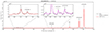 |
Fig. 1. Observed spectrum of Mrk 573 (black solid line). The LZIFU emission line fit (red) is superimposed to the dashed line which represents the stellar continuum fit. |
For red lines fluxes, including Hαλ6563Å and He Iλ5876Å, we performed one, two and three component fits to the combined spectrum, where the optimal number of components was evaluated using the likelihood ratio test with a critical threshold of 0.01 (e.g., Ho et al. 2016). A 5th-order additive polynomial was included in the stellar continuum fit to correct for flux calibration errors. We then repeated this process on the B3000 spectrum in order to obtain [O III] λ5007Å, Hβλ4861Å, Hγλ4340Å and [O III] λ4363Å fluxes. For these fits, a 12th-order additive polynomial was included in the stellar continuum fit to correct for flux calibration errors, and a 12th-order additive polynomial was included during the emission line fit to compensate for residuals due to stellar template match.
Visual inspection revealed significant stellar template mismatch in some objects in the wavelength range encompassing the [Ar IV] doublet lines. We therefore ran a series of tailored fits to obtain fluxes for these weak lines. Due to the low S/N of these lines, they were fitted with only a single Gaussian component to avoid introducing additional systematic errors. We first attempted to obtain [Ar IV] fluxes from the 1-component fits to the B3000 spectra discussed in the paragraph above, where visual inspection was used to assess the quality of the fits. If they were deemed unsatisfactory, we ran a second fit on a smaller wavelength range encompassing the [Ar IV] lines, including 3rd-order polynomials during the stellar continuum and emission line fits, where the order was reduced from 12 to compensate for the smaller wavelength range.
There was a subset of nine objects for which visual inspection of the [Ar IV] fits from both methods described above was not adequate. In these galaxies, the structure of the noise and/or the continuum shape underneath the [Ar IV] doublet and/or the faintness of the [Ar IV] lines (in particular λ4711Å) led to severe systematic errors in the LZIFU fits. For these objects, we manually measured the flux of each [Ar IV] line by fitting a single Gaussian to each line, and by requiring the two doublet lines to have consistent FWHM within the errors. As an additional test, we measured the fluxes simply by integrating the flux underneath each line profile after subtracting the stellar continuum fit generated by LZIFU. The continuum level and shape were also defined separately for each individual emission line. Because in these objects the shape and level of the continuum are the main source of uncertainty, in particular due to the undulating stellar contribution, different assumptions had to be made. The reported flux errors in these affected objects account for the dispersion of the flux values from both methods.
3.2.2. Extinction correction of the measured line fluxes
All emission line fluxes were corrected for extinction intrinsic to the AGNs using the Hα and Hβ fluxes. The internal galaxy AV was computed using the Fitzpatrick (1999) extinction curve with R(V) = 3.1 and assuming an intrinsic Balmer decrement Hα/Hβ of 3.1, as is appropriate for regions dominated by the hard ionizing spectra of AGNs (Dopita et al. 2015; Thomas et al. 2017).
3.2.3. Deblending of [Ar IV] λ4711Å due to weak He Iλ4713Å and [Ne IV] λλ4715Å lines
Following the dereddening of line ratios, the next step consisted of deblending the observed [Ar IV]+ λ4711Å line5, which is blended with the much weaker He Iλ4713Å line, as pointed out by Kewley et al. (2019), as well as with the [Ne IV] λλ4715Å line. We note first that, in our LZIFU fits, we did not separately fit the weak He Iλ4713Å and [Ne IV] λλ4715Å lines, which are blended to the dominant [Ar IV] λ4711Å line. The reason is that in the majority of galaxies in our sample, the magnitude of the stellar template mismatch exceeds the amplitude of these very faint lines. Additionally, at the resolution of the B3000 spectra, given the width of the line profiles, the [Ne IV] λλ4715Å lines are fully blended with the [Ar IV] λ4711Å line and as a result, the fluxes of both lines would be poorly constrained were they to both be included in the fit. This is the reason for adopting the deblending procedure described in Appendix B, which relies on measurements of the He I/[Ar IV] (λ5876Å/λ4740Å) ratio as well as of the [Ne IV]/[Ar IV] (λλ4725Å/λ4740Å) ratio when the [Ne IV] λλ4725Å doublet is detected. Neither deblending corrections are sensitive to the plasma temperature. Visual inspection of the spectra revealed that five objects (ESO 138-G01, IC 2560, NGC 3281, NGC 4939 and NGC 5506) showed prominent [Ne IV] λλ4725Å emission. In these galaxies, the [Ne IV] λλ4725Å fluxes (or upper limits, when the S/N was poor) were estimated by manually fitting a single Gaussian profile as done for the [Ar IV] λ4740Å line in order to estimate the level of contamination of the [Ar IV] λ4711Å flux by the [Ne IV] λλ4715Å doublet. Examples of the LZIFU fits in the region of the He IIλ4686Å and [Ar IV] doublet lines are shown in Fig. 2 for six objects.
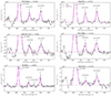 |
Fig. 2. Spectra showing the [Ar IV] doublet lines of six Seyfert 2s (black solid line) from our sample after subtraction of the stellar and AGN continuum fit. From left to right: NGC 5643, Mrk 573, ESO 137-G34, NGC 3393, IC 2560 and Mrk 1210. The LZIFU emission line fit (magenta line) is superimposed to each spectrum. |
3.2.4. Line ratios from the high excitation S7 Seyfert 2 sample
In Table 1, we indicate for each object the aperture that was selected (Col. 3), the object redshift (Col. 4), the extinction values AV (Col. 5) inferred from the observed Balmer decrement, and finally the reddening corrected ratios of [O III] (λ5007Å/λ4861Å; Col. 6) and He II/Hβ (λ4686Å/λ4861Å; Col. 7).
In Table 2, we subsequently list the dereddened ratios of [O III] (λ4363Å/λ5007Å; Col. 3), [Ar IV]+ (λ4711Å+/λ4740Å; Col. 4), RHe/Ar (λ5876Å/λ4740Å; Col. 5) and [Ne IV]/[Ar IV] (λλ4725Å/λ4740Å; Col. 7). The subindex + refers to blending being present in the [Ar IV] λ4711Å line measurement due to the unresolved He Iλ4713Å and [Ne IV] λλ4715Å lines. The adopted procedure for deblending [Ar IV]+ (λ4711Å+/λ4740Å) is described in Sect. 3.2.3 using the He Iλ5876Å and [Ne IV] λλ4725Å lines, respectively. This correction is relatively minor since the inferred intensity of the He I (λ4713Å) line turns out typically to be only ≃12 ± 5.3% of the (deblended) [Ar IV] λ4711Å line flux. Finally, the deblended [Ar IV] ratios that were used to constrain the NLR densities are listed in Col. 9 of Table 2.
NLR temperatures derived using the reddening-corrected ratios for our sample extracted from the S7 survey.
In Fig. 3 we present, as a function of the aperture D (in units of kpc) projected on the sky, the distribution of the following four quantities from Tables 1 and 2: the dust extinctions AV and the three dereddened ratios of ROIII, [O III] (λ5007Å/λ4861Å) and [Ar IV]+ (λ4711Å+/λ4740Å). The red dots correspond to the three objects identified as outliers due of their anomalous ROIII ratios (see Sects. 3.3 and 3.5). No significant correlation was found between AV or the line ratios with the aperture size, as indicated by the Pearson correlation coefficients (P), which are all negligible (< 0.5). We concluded that the use of distinct aperture sizes did not have any significant impact on the results presented in this work.
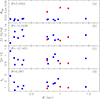 |
Fig. 3. Pearson correlation coefficients for our sample of high excitation Seyfert 2s from the S7 survey. From bottom to top panel, the V band extinction in magnitudes AV and the extinction corrected values of observed [Ar IV]+ (λ4711Å+/λ4740Å), [O III] (λ5007Å/λ4861Å) and ROIII line ratios (Tables 1 and 2) versus the aperture D (in kpc) used to extract the spectra. The value of the Pearson correlation coefficient (P) is indicated in each panel. The red points identify the three outliers discussed in Sect. 3.5. |
3.3. Distribution of ROIII ratios among S7 high excitation Seyfert 2s
The dereddened ratios of [O III] (λ5007Å/λ4861Å) versus ROIII of our S7 survey sample are illustrated in Fig. 4a. Unlike quasars which extends over a wide range in ROIII (light-gray open squares), our S7 sample of 13 Seyfert 2s (blue dots) cluster around a similar ROIII value. A navy colored circle (labeled S7) represents their average ROIII of 0.0146 ± 0.0020. The circle’s radius σs = 0.057 dex represents the sample dispersion of the ROIII ratios. The three objects labeled “outliers” in Tables 1 and 2 stand out at much higher ROIII values, beyond seven times the sample dispersion σs. Some of their characteristics are discussed in Sect. 3.5.
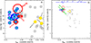 |
Fig. 4. Dereddened NLR ratios of [O III]/Hβ versus ROIII. Left panel a: blue dots represent the line ratios of 13 Seyfert 2s from the S7 survey sample which are listed in Table 1. Their average ROIII ratio is 0.0146 ± 0.0020, which is represented by the navy colored circle whose radius of 0.057 dex corresponds to the dispersion of the measurements. The yellow filled dots identifies the three outlier Seyfert 2s: ESO 138-G01, Mrk 1210 and NGC 4507 (labeled a, b, c in Table 1). Three complementary Seyfert 2 samples are represented by red open symbols: (1) the average of seven Seyfert 2s from Kos78 studied by BVM (large red circle), (2) the average of four Seyfert 2s from Be06b (small open circle with dispersion bars), (3) the high excitation Seyfert 2 subset a41 from Richardson et al. (2014; open red diamond). The light-gray open squares represent the ratios of Type I AGNs measured by BL05. Right panel b: a similar graph but with an expanded scale in order to cover the full range of ratios observed by BL05 among 30 quasars. The light-gray open triangles represent the four narrow-line Seyfert 1 galaxies observed by RA00. Both BL05 and RA00 subtracted the BLR profile component from Hβ before deriving the [O III]/Hβ ratio. The light-green filled symbols represent the spatially resolved ENLR measurements from three studies: (1) the average of two Seyfert 2s and two NLRGs (small light-green dot) from BWS, (2) the integrated long-slit spectrum of the Seyfert 2 IC 5063 from Be06b (pentagon), (3) the average of seven spatially resolved optical filaments of the radio-galaxy Centaurus A (light-green triangle) from Mo91. The blue segmented arrow at the top describes the effect of collisional deexcitation on the ROIII ratio for a 13 000 K isothermal plasma whose density is increased to successively larger values, from 102 to 106.5 cm−3. |
It is noteworthy that a similar clustering takes place among the seven high excitation Seyfert 2s studied by BVM8 using measurements from Kos78. Their average ROIII is represented by the red circle centered at ROIII = 0.0168 and whose radius of 0.088 dex represents the sample’s RMS dispersion.
Interestingly, other samples show similar trends. For instance the average of the four Seyfert 2s studied by Bennert et al. (2006b, hereafter Be06b), which is represented by the small red open circle with dispersion bars representing the RMS dispersion. A much larger sample of Seyfert 2s is represented by the red open diamond which corresponds to the high excitation subset a41 extracted from the SDSS survey by Ri14. Unfortunately, only the [Ar IV] λ4711Å line was extracted by Ri14.
To illustrate the effect of collisional deexcitation on the ROIII ratio, the blue horizontal arrow in Fig. 4b represents the ROIII ratios of a 13 000 K isothermal plasma in which the density successively takes on values that increase from 102 cm−3 up to 106.5 cm−3. For NLR densities above 105 cm−3, we can expect the ROIII ratios to take on much higher values as is indeed observed among Type I AGNs from the BL05 quasar dataset, which are represented in Fig. 4b by light-gray open squares. On the other hand, for the S7 Seyfert 2s, the measured [Ar IV] doublet ratios from Table 2 show evidence that the observed NLR have densities ≪105 cm−3, in which case we can trust the ROIII ratio as a direct temperature estimator.
3.4. Comparison with ENLR observations
Superposed in Fig. 4b are the ratios observed from the spatially resolved emission component of AGNs, the ENLR. They are represented by three light-green filled symbols which were extracted from the following samples: (i) the average of two Seyfert 2s and two NLRGs (filled dot) from Binette et al. (1996, hereafter BWS), (ii) the long-slit observations of the Seyfert 2 IC 5063 by Be06b (pentagon), and (iii) the average of seven spatially resolved optical filaments from the radio-galaxy Centaurus A (filled square) from Morganti et al. (1991, hereafter Mo91).
A remarkable feature is the near superposition of the ROIII ratios from ENLR measurements with those of the NLR of Seyfert 2s. Detailed modeling with photoionization calculations (e.g., Tadhunter et al. 1994; Bennert et al. 2006a,b) indicated that the ENLR emission occurs at low plasma densities (ne < 1500 cm−3). The simplest interpretation for the coincidence in position in Fig. 4b of the ROIII ratios from the ENLR and the NLR data sets is that in both cases the emission corresponds to relatively low densities in which collisional deexcitation is not significant. Interestingly, the six quasars from the BL05 sample with the lowest values in ROIII share positions relatively close to that of the NLR and ENLR measurements. We would propose that the accumulation of AGNs at a similar position on the left is most likely representing a floor AGN temperature where collisional deexcitation of ROIII is not significant.
3.5. The three outliers
The three Seyfert 2s labeled outliers (yellow filled dots in Fig. 4) correspond to the galaxies ESO 138-G01, Mrk 1210 and NGC 4507. Although the densities inferred from the [Ar IV] doublet are comparable to the other sample objects, their ROIII values are significantly higher than the average of the other nuclei. They depart from the averaged blue dots position in Fig. 4a by more than seven times the cluster dispersion in ROIII. This could suggest that their plasma is much hotter (∼20 000 K), possibly as a result of fast shocks (Binette et al. 1985; Sutherland et al. 2003), or alternatively could be caused by a dual-density distribution where some plasma components might possess densities above ≳106 cm−3 as was considered by BVM to account for the high ROIII values encountered in 3 luminous QSO 2s where they had measurements of the [Ar IV] doublet. Among the optical [O III] and [Ar IV] lines, the only one not affected by collisional deexcitation in this case is the [O III] λ4363Å line since its critical density is much higher, at 4.5 × 107 cm−3. With a dual-density distribution where a very dense component is present, the integrated [Ar IV] doublet ratio would be relatively unaffected by such high density component.
Interestingly, a polarized BLR component has been detected in Mrk 1210 (Tran et al. 1992; Tran 1995; Storchi-Bergmann et al. 1998) and NGC 4507 (Moran et al. 2000). They were classified as S1h by Véron-Cetty & Véron (2010, 2006). They possibly represent borderline cases between Type I and II AGNs. With respect to ESO 138-G01, the detailed analysis of Alloin et al. (1992) reveals a strong stratification of the emitting gas clouds that correlates with the density as well as with the presence of high ionization Fe species.
Mrk 1210 presents a very rich coronal line spectrum that includes [Si X], which is a very high excitation line not frequently detected (Mazzalay & Rodríguez-Ardila 2007). ESO 138-G01 is also a strong coronal line emitter. It was classified as a “coronal-line forest active galactic nuclei” (CLIFF AGNs), which are characterized by strong very high ionization lines, in contrast to what is found in most AGNs (Cerqueira-Campos et al. 2021).
Mazzalay et al. (2010) studied NGC 4507 as part of a sample of Seyferts selected on the basis of previous detection of coronal lines. It was originally classified as a Seyfert 2 (Durret & Bergeron 1986), but later reclassified as S1h (i.e., Seyfert 1.9) by Véron-Cetty & Véron (2006) because of the presence of a weak broad Hα in its spectrum.
Using observed IRAS mid-infrared and far-infrared continuum fluxes at 25 and 60 μm, Meléndez et al. (2008b) derived the spectral indices α25 − 60 of 98 Seyfert nuclei. The average index values reported were α25 − 60 = −1.5 ± 0.1 for Seyfert 2s and α25 − 60 = −0.8 ± 0.1 for Seyfert 1s. Interestingly, for the two outliers9 Mrk 1210 and NGC 4507, the average index is −0.46, indicating that the continuum emission originates from dust that is hotter than in typical Seyfert 2s.
4. A combined temperature-density diagnostic
The utility of “diagnostic” line ratios such as ROIII, [Ar IV] (λ4711Å/λ4740Å) or [S II] (λ6716Å/λ6731Å) is that they are independent of metallicity since they involve ions of the same species. The [Ar IV] density diagnostic for instance depends on density and negligibly on temperature while the ROIII diagnostic ratio depends on both except in the low density regime (ne ≲ 103 cm−3; Osterbrock 1989) where it varies according to temperature. Therefore, in order to reliably measure the NLR temperature, a handle on the plasma density is required, which is our motivation for focusing on data sets where the [Ar IV] doublet is observed. A concern is that while the ROIII ratio remains a valid temperature indicator up to densities of ∼108 cm−3 the [Ar IV] doublet ratio saturates and becomes progressively insensitive to the density beyond 105 cm−3. Hence, in situations where the observed ROIII ratio represents the emission from multiple density components that extend beyond ≳106 cm−3, the [Ar IV] doublet would not detect the higher densities while the ROIII ratio would increase as a result of collisional deexcitation, whether or not the temperature remains the same across the different components.
Our goal is to determine the temperature of the observed NLR by combining the ROIII and [Ar IV] diagnostics and requiring that the inferred temperature and density simultaneously reproduce the dereddened [Ar IV] (λ4711Å/λ4740Å) and ROIII ratios of the S7 survey sample. First, we consider in Sect. 4.1 the simplest case of a single density isothermal plasma. The algorithm OSALD as described in Appendix C of BVM proceeds iteratively using a nonlinear least squares fit method to determine which temperature and density are required to simultaneously reproduce the ROIII and [Ar IV] ratios. Subsequently in Sect. 4.2 we assume a power-law distribution of the density that extends up to the density ncut which is determined iteratively using OSALD.
4.1. Temperatures inferred from the single density case
In Tables 1 and 2, the Seyfert 2 sample follows an ascending order in the densities that were inferred from the [Ar IV] doublet. These extend from 6000 up to 54 000 cm−3. The average temperature for the sample of 13 Seyfert 2s is  K (that is, ±0.023 dex). We find remarkable that the S7 Seyfert 2s clustered over such a narrow range in temperature values. The average temperature inferred is comparable to the value of 13 480 ± 1180 K derived by BVM for the seven Seyfert 2s observed by Kos78.
4.2. OSALD algorithm: A power-law density distribution
The algorithm10 OSALD was developed to explore the effect of collisional deexcitation on the [O III] and [Ar IV] lines when the densities extend over a wide range of values from 102 cm−3 up to a cut-off density, ncut. The intention is to implement the case of NLR densities that increase radially toward the ionizing source as was observed in ENLR studies (e.g., Bennert et al. 2006b).
4.2.1. Transposition to a simplified spherical geometry
The algorithm consists in integrating the line emission measures11 of an isothermal multi-density plasma (hereafter MDP) of uniform temperature Te. The calculations can be transposed to the idealized geometry of a spherical (or conical) distribution of ionization bounded clouds whose densities n decrease as r−2. The clouds can be visualized as being radially distributed along concentric shells of negligible covering factor. The weight attributed to each plasma density component is set proportional to the covering solid angle12Ω(n) subtended by each plasma shell. In the case of photoionization models, such a cloud distribution would result in a constant ionization parameter Uo and the integrated columns NXk of each ion k of any cloud would be to a first order constant. For the sake of simplicity, to describe Ω(n) we adopt a power law (n/nlow)ϵ, which extends from nlow = 102 cm−3 up to ncut. If we transpose this to a spherical geometry where both Uo and Ω are constant (i.e., ϵ = 0), the area covered by ionization-bounded emission clouds would increase as r2, thereby compensating the dilution of the ionizing flux and the density fall out (both ∝r−2). In this case, the weight attributed by OSALD to each shell is the same, otherwise when ϵ ≠ 0 the weight is simply proportional to Ω(n). MDP calculations are not a substitute to photoionization calculations. They serve as diagnostics that could constrain some of the many free parameters that characterize multidimensional NLR models, including the option of a nonuniform dust distribution where the opacity correlates with density, that is with r, as was explored by BVM. The line ratios used as target in their diagnostics were not dereddened but were part of the simultaneous modeling of the [O III], [Ar IV], He I and H I Balmer lines. In the current work, we only consider reddening corrected line ratios and assume a distribution of densities that extends up to a sharp cut-off. The latter is a free parameter, which is constrained through line ratio fitting using OSALD.
To guide us in the selection of ϵ, we followed the work of Be06b who determined that, for a spectral slit radially positioned along the emission line cone, the surface brightness of the spatially resolved ENLR is seen decreasing radially along the slit as rδ (with δ < 0), where r is the projected nuclear distance on the sky. From their [O III] λ5007Å and Hα line observations of Seyfert 2s, Be06b derived average index values of δ[OIII] = −2.24 ± 0.2 and δHα = −2.16 ± 0.2, respectively. Let us assume that such gradient extends inward, that is, crosswise the unresolved NLR. For our assumed spherical geometry where the Hα luminosity across concentric circular apertures behave as r−2ϵ, ϵ is given by −(1 + δ)/2. Hence the value inferred for ϵ, which describes how the covering factor varies with density, is +0.6 in order that a long slit projected onto our assumed spherical geometry reproduce the δ[OIII] value reported by Be06b. To derive the optimal values for the selected input parameters that would reproduce as closely as possible the [O III] and [Ar IV] target line ratios, OSALD proceeds iteratively via a nonlinear least squares fit method as described in Appendix C.5 of BVM.
4.2.2. Temperatures inferred from a density stratified plasma
The cut-off densities ncut inferred from the algorithm OSALD for the case of a power-law density distribution are given in Col. 3 of Table 3. These extend from 4075 up to 1.14 × 105 cm−3. What governs the integrated line ratios, however, are the mean plasma densities. The luminosity weighted densities  , in Table 2 (Col. 4), range from 2430 up to 66 700 cm−3. The average temperature for the whole sample,
  , is 12 961 ± 711 K, which is essentially the same value as the single density case of Table 2. The main reason is that the ROIII ratio varies relatively little across the density interval covered. For instance, for the densest object, IC 2560, the shell densities of the fitted power law cover the range 102 to 1.14 × 105 cm−3 and the ROIII ratios calculated by OSALD across the different shells span over the range 0.01252 to 0.01547.
Changes in NLR temperatures assuming a power-law density distribution.
As shown by the differences in temperature ΔTiso (Col. 5) between the values derived from OSALD and those of the single density case, the temperatures  for the first 10 objects are essentially the same as those derived assuming a single density
  . For the most part ΔTiso is negligible and likely represents numerical noise from the iterative procedure, except possibly for the last three objects labeled 11–13.
5. Comparison with densities inferred from outflow studies
AGNs outflows are inhomogeneous and they extend over a large range of densities and geometries. Consequently the outflow rates, gas masses and kinematics that are inferred depend strongly on how the gas densities are estimated. We now review some of the techniques used.
5.1. The use of trans-auroral and auroral lines
Evidence that the densities inferred from the red [S II] doublet are not representative of the plasma observed in the NLR, or even the ENLR plasma, has been demonstrated in studies of outflows observed in Type II AGNs where the emission line profile was fitted using a central component to represent the stationary plasma and one or more velocity shifted profiles that fitted the asymmetric component, the latter being interpreted as out-flowing winds. A technique developed by Holt et al. (2011) to determine NLR densities in Type II AGNs made use of the trans-auroral and auroral [S II] and [O II] lines. The [S II] (λλ4069,76Å/λλ6716,31Å) and [O II] (λλ3726,29Å/λλ7320,31Å) ratios are sensitive to densities up to 106 cm−3 and when both ratios are combined, one can simultaneously determine the plasma density and the intervening dust extinction. The densities inferred by Rose et al. (2018) and Spence et al. (2018) for the outflowing plasma13 component in ten Type II ULIRGs ranged from 103 to 104.6 cm−3. For the ULIRG Pks B1345+12, the densities inferred by Holt et al. (2011) from the intermediate and very broad NLR profile components were 104.2 and 105.5cm−3, respectively, while for the AGN Pks B1934-63 the densities inferred by Santoro et al. (2018) for the corresponding components were 104.6 and 105.5cm−3, respectively.
Davies et al. (2020, hereafter Da20) similarly used the trans-auroral and auroral [S II] and [O II] lines to evaluate the densities of eight Type II objects14. They calibrated their density diagnostic diagram using photoionization calculations that took into account differences in temperature and ionization of the regions which emit the trans-auroral and auroral lines. The densities encountered ranged from 103.0 to 103.6 cm−3. The median density for the sample was 1900 cm−3, which is more than five times higher than the median density inferred from the [S II] λλ6716,31Å doublet measurements from their sample. After comparing how the red [S II] λλ6716,31Å doublet and [O III]/Hβ ratios varied across their respective profiles, Da20 found no evidence in their sample of an emission component that could be specifically associated to the systemic velocity (as defined by the stellar absorption lines). They commented that the multiple Gaussians from their profile fits do not represent distinct outflow components and for this reason they use the full integrated line fluxes in their analysis of the outflow densities.
5.2. The ionization parameter estimation method
In objects where no reliable density diagnostic is available, Baron & Netzer (2019) proposed a method which they labeled “ionization parameter estimation”. By comparing the [O III]/Hβ (λ5007Å/λ4861Å) and [N II]/Hα (λ6583Å/λ6563Å) ratios with the predictions of photoionization calculations, one can attribute a value to the ionization parameter U. The plasma density ne is then derived from the expression  where QH is the photon luminosity rate from the ionizing source, which is determined by estimating the AGN bolometric luminosity assuming a standard SED. To determine ne, this technique is only applicable to spatially resolved measurements as it requires knowledge of the distance remi separating the point source nucleus from the position of the line measurement (along the slit or at a given IFU). However, a novel technique to estimate remi within the unresolved nuclear NLR was proposed by Baron & Netzer (2019). It consisted in evaluating the mean location of the dust responsible for the mid-infrared excess emission from the outflows, which were measured using the 2-Micron All-Sky Survey (Skrutskie et al. 2006). For their sample of 234 ionized outflows in Type II AGNs extracted from the ALPAKA catalog (Mullaney et al. 2013), the mass-weighted average dust location, rdust, was ≈200 pc ±0.25 dex (Fig. 6 of Baron & Netzer 2019). The mean density that characterized their whole sample was 104.5 cm−3, that is more than an order of magnitude above the values inferred from the [S II] λλ6716,31Å doublet.
The density method of Baron & Netzer (2019) based on the estimated ionization parameter was incorporated to the Da20 study mentioned above and applied to 11 Type II AGNs of their sample. For their sample which integrated the emission of the nucleus with an IFU of 1.8″ × 1.8″, they estimated the projected size of the nucleus distance as corresponding to half the IFU size, that is 0.9″. The effect of projection was subsequently taken into account by multiplying the projected radius (in pc) by a factor of 1.4, which corresponds to a disk inclination of 45°. The densities they encountered extended from 102.9 to 104.8 cm−3. The median density for the whole sample is 4800 cm−3 while the corresponding value using the trans-auroral lines method discussed above is 1900 cm−3. As recognized by Da20, this method is most suited to spatially resolved data, where one can obtain measurements at a known projected distance remi from the AGN nucleus. Since their dataset consisted of spatially integrated nucleus measurements, Da20 recommended one should make use of the derived densities in a statistical sense rather than focusing on individual values.
5.3. Benefits of high spatial resolution HST observations of outflows
Reaching much smaller projected nucleus distances remi is possible by using observations from the Space Telescope Imaging Spectrograph (STIS), as shown by Revalski et al. (2021). Spatially resolved observations are essential for localizing AGN feedback and determining accurately the wind kinematics. Observations of the [Ar IV] doublet was reported by Revalski et al. (2018) in only one object, Mrk 573. In their study, the authors combined with varying weights three different photoionization models corresponding to a high, intermediate and low U values at each location along the STIS slit observations as well as of the DIS long-slit from the Apache Point Observatory (APO). The line ratios with respect to Hβ at each radial location were generally well reproduced (their Fig. 9) across the whole ENLR except for the two [O I] optical lines and the two [Ar IV]/Hβ ratios, although it had relatively little impact on their determination of the peak outflow velocity as well as other global wind kinetics. At only two positions along the HST-STIS slit do we suggest a distinct interpretation concerning the densities inferred, that is at +0.05″ and −0.05″ from the nucleus, where their intermediate U model favored densities of 105.1 and 105.3 cm−3 with a relative flux weight of 50% in both cases with respect to the high and low ionization models. Because of likely optical blurring within the 0.2″ slit width, it is not possible in our opinion to confirm the value of remi, on which the model densities so close to the nucleus are based. Using OSALD, the densities we infer at the corresponding positions from the [Ar IV] doublet ratios of Re18 are 22 600 and 4220 cm−3, which are values significantly lower. The corresponding temperatures inferred from the ROIII ratios are 16 600 and 13 800 K, respectively15.
More recently, for six Seyfert 2s, Revalski et al. (2022) compared the densities derived from their multicomponent photoionization models to other techniques that involve more assumptions about the gas physical conditions, but require less data and modeling (Revalski et al. 2022). For instance, the three ionization parameter values assumed (log U = [ − 1.5, −2.0, −2.5]) were the same at each radial location for all six objects. A good match of the observed line ratios along the slit was obtained although the assumed remi values at the position of the nucleus remained unconstrained and the caveat mentioned above by Da20 concerning the densities inferred from a spatially unresolved remi value would still apply to their analysis, as acknowledged by Revalski et al. (2021). If we exclude those calculations positioned at the closest distance from the SMBH, the densities inferred at the other radii, among their sample of six Seyfert 2s, all fall below 105 cm−3 except Mrk 3.
6. Standard photoionization calculations
Having shown that collisional deexcitation of the [O III] optical lines is relatively insignificant among a large fraction of Seyfert 2s from the S7 sample, we first illustrate the difficulty in reproducing the typical ROIII ratio observed in Seyfert 2s and subsequently explore in Sect. 7 possible solutions.
6.1. Standard input parameters for MAPPINGS Ig calculations
Most model parameters share similar values across the calculations presented below and in Sect. 7. With respect to the plasma metallicities, it is generally accepted that gas abundances of galactic nuclei are significantly above solar values. The values we adopted below correspond to 2.5 Z⊙ as in BVM, a value within the range expected for galactic nuclei of spiral galaxies as suggested by the Dopita et al. (2014) landmark study of the Seyfert 2 NGC 5427 using the Wide Field Spectrograph (WiFeS: Dopita et al. 2010). High metallicity values are shared by other observational and theoretical studies that confirm the high metallicities of Seyfert nuclei (Storchi-Bergmann & Pastoriza 1990; Nagao et al. 2002; Ballero et al. 2008). Our selected abundance set is twice the solar reference set of Asplund et al. (2006), that is, with O/H = 9.8 × 10⁻⁴, except for C/H and N/H which reach four times the solar values owing to secondary enrichment. We can expect the enriched metallicities of galactic nuclei to be accompanied by an increase in He abundance. We followed a suggestion from David Nicholls (priv. comm., ANU) of extrapolating to higher abundances the metallicity scaling formulas that Nicholls et al. (2017) derived from local B stars abundance determinations. At the adopted O/H ratio, the proposed scaling formula described by Eq. (A1) in Appendix A.c of Binette et al. (2023, hereafter BK23) implies a value of He/H = 0.12, which is mildly higher than the ratio of 0.103 adopted by Ri14. Our calculations are dustfree and assume a simple slab geometry in which the plasma is radiation-bounded and exposed to ionizing radiation emitted by the accretion disk assuming an ionization parameter defined as  , where ϕ0 is the ionizing photon flux impinging on the photoionized slab,
  the hydrogen density at the face of the slab and c the speed of light.
6.2. Thermal ionizing continuum
The ionizing radiation from the nucleus was assumed to originate from thermal emission by gas accreting onto a supermassive black hole. Although thermal in nature, the spectral energy distribution (SED) is broader than a blackbody since the continuum emission is considered to take place from an extended disk that covers a wide temperature range. In their photoionization models, Fg97 and Ri14 assumed a SED where the dominant ionizing continuum corresponds to a thermal distribution of the form
 (1)
(1)
where αUV is the low-energy slope of the “big bump”, which is typically assumed to be αUV = −0.3, and Tcut is the temperature cut-off. The values for Tcut adopted by Fg97 and Ri14 are 106.0 and 105.62 K, respectively. Both distributions are shown in Fig. 5 (black dashed lines). The thermal component dominates the ionizing continuum up to the X-ray domain where a power-law of index −1.0 takes over. For each SED hereafter considered, we impose an αOX of −1.35.
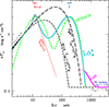 |
Fig. 5. Ionizing SEDs in νFν units: (1) the SED adopted by Fg97 for their LOC calculations using Tcut = 106.0 K (black long-dash line), (2) the optimized SED of Ri14 with Tcut = 105.62 K (black dotted short-dash line), (3) the double-bump distribution La |

6.3. Standard photoionization models
Assuming the Fg97 SED, a sequence of isochoric (i.e., constant density) photoionization models was calculated with the code MAPPINGS Ig (see updates in BK23, BVM and Appendices B and C of current paper) are shown in Fig. 6 (magenta line) where Uo increases in steps of 0.33 dex, from 0.01 (the gray dot) up to 0.46. In each model, the same frontal16 plasma density of  cm−3 is assumed. A square identifies models with Uo = 0.1. The whole sequence predicts ROIII values significantly lower than observed in the S7 survey (navy circle) or the Kos78 dataset (red circle) or the high excitation subset a41 from Ri14 (red diamond). The softer Ri14 SED shown in Fig. 5 results in even lower ROIII values, as shown by the yellow line sequence in Fig. 6. Either sequence illustrates the TE problem reported by various authors (e.g., Storchi-Bergmann et al. 1996; Bennert et al. 2006a; Villar-Martín et al. 2008; Dors et al. 2015, and BVM).
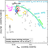 |
Fig. 6. Dereddened NLR ratios of [O III]/Hβ versus ROIII for the same observational dataset as in Fig. 4. Two ionization parameter sequences of isochoric photoionization calculations with a frontal density of |


7. Possible solutions to the TE problem
Finding the cause of why model calculations predict values of ROIII ratios significantly lower than observed is the next step. Except for the three outliers, where a high density NLR component is likely present, we considered that collisional deexcitation of the [O III] optical lines is unlikely the cause as discussed in Sect. 5, at least among the current sample of 13 Seyfert 2s where we could measure the [Ar IV] doublet as well as for the seven Seyfert 2s from the Kos78 dataset (BVM). We present below a few alternative solutions but do not rule out the existence of alternative interpretations that should eventually be explored. The calculations presented below all assume the same metallicities of 2.5 Z⊙ and, except in Sect. 7.1, the same ionizing SED of Fg97 with Tcut = 106.0 K.
7.1. Double-bump continuum distributions
As pointed out by Lawrence (2012, hereafter La12), AGNs seem to show a universal near-UV shape, reaching a maximum in νFν at a wavelength of around 1100 Å, regardless of luminosity or redshift (cf. Zheng et al. 1997; Telfer et al. 2002; Scott et al. 2004; Binette et al. 2005; Shang et al. 2005). To address the TE problem, La12 explored the possibility that a population of internally cold very thick (NH > 1024 cm−2) dense clouds (n ∼ 1012 cm−3) covers the accretion disk at a radius of ∼30 Rs from the black-hole, where Rs is the Schwarzschild radius. The cloud’s high velocity turbulent motions blur its line emission as well as reflect the disk emission, resulting in a double-peaked SED superposed to the reflected SED. The first peak at ∼1100 Å represents the clouds reprocessed radiation while the second corresponds to the disk radiation reflected by the clouds, which La12 positioned at ∼40 eV. The main advantage of this distribution is its ability to account for the “universal knee” observed at 12 eV in quasars. As shown by BVM, however, the resulting SED did not significantly increase the temperature of the photoionized plasma. The authors argued that the second peak must be shifted to much higher energies in order to reproduce the observed ROIII ratio and thereby resolve the TE problem.
To achieve this, BK23 proceeded as follows. First, they extracted a digitized version of the published La12 SED and to eliminate the 40 eV peak they extrapolated the declining segment of the first peak, as represented by the red dotted line in Fig. 5. For the second peak,  , they adopted the formula, ναFUVexp(−hν/kTcut) (i.e., Eq. (1)). All the double-bump SEDs which they explored were obtained by simply summing both distributions:
 (2)
(2)
where  is the renormalization factor which we define at hνpk1 = 12 eV, the energy where the first peak reaches its maximum in νFν. The position and width of the second peak depend on both parameters αFUV and Tcut while its intensity is set by the parameter
  . After experimenting with different shapes and positions for the second peak, it was found that the presence of a deep valley at ≃35 eV increased the heating rate due to He+ photoionization, hence generating a higher plasma temperature (i.e., a higher ROIII ratio).
After comparing the plasma temperatures reached when different combinations of the parameters Tcut, αFUV and  were considered, BK23 concluded that the optimal position for the second peak is ≈200 eV in order that the ROIII ratio from photoionization models reach the observed values. Moving it to higher values was not an option as it generated an excessive flux in the soft X-rays that is not observed in Type II AGNs. The height of the peak is set by the scaling parameter
  . For a given value of αFUV, an increase of
  or Tcut favors higher values of ROIII. However, the optimization of the SED parameters must ensure that it does not generate an excessive flux beyond 500 eV in the soft X-rays.
The first SED described by BK23, labeled  , assumes the value αFUV = +0.3, which is similar to the standard Shakura-Sunyaev accretion disk model17 (Shakura & Sunyaev 1973; Pringle 1981; Cheng et al. 2019) with αFUV = 1/3. The optimized values of the other parameters were Tcut = 1.6 106 K with a scaling factor
  . Increasing αFUV resulted in a narrower second peak, which prevents having a conflict with the soft-X ray observational limits. The second SED proposed by BK23, La
 , assumed a much larger αFUV of +3. In order that the second peak occurred at essentially the same energy as in the previous SED, the parameter Tcut had to be reduced to 0.5 106 K with a scaling parameter
  of 0.001.
7.1.1. Calculations using the double-bump SED La
For the current work, we opted for an intermediate case where αFUV = +1.0. The resulting SED is labeled La in Fig. 5 (cyan solid line). The optimized values for the other parameters are Tcut = 1.0 106 K with a scaling factor
  . These parameter values ensured that the predicted flux beyond 500 eV did not exceed the soft X-rays measurements. For illustrative purposes, we show in Fig. 5 the average soft excess component observed with XMM-Newton (magenta line) by Piconcelli et al. (2005, hereafter Pi05). It corresponds to the best-fit average of 13 quasars with z < 0.4 using the parameters from Table 5 of Pi05, as described in Haro-Corzo et al. (2007). It has been rescaled so as to reproduce an αOX of −1.35 with respect to the first bump. We note that the dotted section below 600 eV is speculative as it is not reliably constrained by the X-ray measurements.
Using MAPPINGS I, we calculated an ionizing parameter sequence assuming a constant density of 102 cm−3 and the same metallicities as defined in Sect. 6.1. The models are represented by the black dotted line in Fig. 6, which shows that the double bump SED has the potential of reproducing the observed ROIII ratios. The He II/Hβ ratio from this sequence is 0.27, which is close to the mean value of 0.24 from the S7 sample in Table 1.
In order to extend our models to Type I AGNs (open gray symbols), we calculated a density sequence along which the density increases in steps of 0.5 dex, from  up to 107 cm−3. These calculations are represented by the cyan solid line in Fig. 6. We selected Uo = 0.3 in order that the models cover the upper envelope of the quasar [O III]/Hβ ratios. Among quasars, the vertical dispersion in the observed [O III]/Hβ ratios is significant. It suggests a significant range in plasma excitation, which can be accounted for using lower values of Uo or dual-density models as explored by BL05.
7.1.2. Possible origin of the double-peak SED
Given that a double-peak SED can solve the [O III] TE problem, it is worth exploring how such a distribution might actually arise in the central regions of quasars. The pertinence of a second peak to describe the harder UV component is provided by studies that attempt to explain the soft X-ray excess in AGNs. Two different processes have been proposed to explain this feature.
The first one postulates the presence of relativistic blurred reflection by ionized plasma (e.g., Ross & Fabian 2005). We note that this mechanism is exactly the same one as proposed by La12, producing a second peak near 40 eV. However, in this case, the relativistic clouds reflecting the disk emission need to be much hotter, with a high degree of ionization, in order to extend its blurred reflection all the way up to the soft X-ray band. As such, these models have the potential to explain at the same time the presence of a second peak near 200 eV, and the soft X-ray excess.
The second mechanism besought to explain the soft X-ray excess proposes comptonization of the accretion disk seed photons by a dual-coronal system (e.g., Done et al. 2012). In this self-consistent accretion model (referred to as OPTXAGN), the primary emission from the disk becomes partly comptonized by an optically thick warm plasma, forming the extreme EUV as well as the soft excess. An example of an OPTXAGN model is represented in Fig. 5 by the light-green dashed curve (see BK23 for more details). The OPTXAGN SED can successfully reproduce the observed ROIII ratio, as shown by the light-green dashed line in Fig. 6, which is a density sequence of isochoric photoionization models similar to the previous La calculations. There are other sets of parameters in the OPTXAGN model that can match our double-peak SEDs, however, they require extreme accretion rates (L/LEdd ≥ 1) that are not proper of Type II objects discussed in this work.
Despite these drawbacks, we note the striking similarity of the OPTXAGN SED with that of La , considering that they were built independently and with completely different scientific motivations. Overall, we find it remarkable that the two most popular mechanisms to explain the presence of the soft X-ray excess (blurred reflection or warm comptonization) might also produce in a natural way the double-peak SED needed to explain the observed ROIII ratios.
7.2. High ionization matter-bounded clouds
Another possibility which benefits from photoionization of He+ consists in high ionization matter-bounded clouds (hereafter MB) as was proposed in the modeling of the NLR and ENLR spectra by BWS, Stasińska (1984), Viegas & Prieto (1992) and Morganti et al. (1991). In their models, BWS truncated the photoionization models at a depth close to the position where most photons with energies above the ionization potential of He+ (54.4 eV) have been absorbed. They considered an ionizing continuum consisting of a power law with Fν ∝ ν−1.3. In the current work, we adopt the thermal distribution of Fg97 with Tcut = 106 K (long-dash line in Fig. 5). Similarly to BWS, our photoionization models were truncated at a depth which is defined by the fraction FMB of the ionizing photons that has been absorbed. We found that calculations with FMB = 0.45 can reproduce the observed ROIII ratios of the S7 sample as indicated below.
7.2.1. Radiation pressure stratified MB component
Rather than assuming an isochoric or isobaric density profile for the MB component, we considered the effect of radiation pressure on the high ionization regions. As shown in Binette et al. (1997), Binette (1998), Dopita et al. (2002), radiation pressure exerted by the progressive absorption of the ionizing photons can induce a density gradient within the photoionized slabs. Binette et al. (1997) have indicated that for high Uo values, the density averaged ionization parameter  across the photoionized slab tended asymptotically toward a constant value where the integrated line ratios to a first order became insensitive to Uo. One important parameter that must be defined is FMB, the fraction of ionizing photons absorbed within MB clouds. Our selected value was inferred from the
  cm−3 MB calculation by determining at which depth (FMB) the integrated ROIII ratio reached 0.015, the average ratio observed among the S7 Seyfert 2 sample. We found that the truncation of the MB component should take place at FMB = 0.45, a similar value to that of BWS of 0.40.
The resulting MB component is represented by the blue continuous line in Fig. 7 along which the frontal density  successively increases in steps of 0.5 dex, starting at 102 cm−3. The gray dotted line shows the calculated line ratios if the same photoionization models were ionization-bounded rather than MB. In this case, the ROIII ratios are significantly lower than the S7 blue circle positioned at 10−1.836, except for the high density models owing to collisional deexcitation.
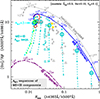 |
Fig. 7. Dereddened NLR ratios of [O III]/Hβ versus ROIII for the same observational dataset as in Fig. 4. The blue solid line represent the sequence of MB models in which the frontal densities varied from |


The matter-bounded component cannot account for the lower excitation emission lines and an additional emission component is required. BWS explored the possibility of combining the emission spectra from both a matter-bounded (MB) and an ionization-bounded (IB) component. The relative proportion of both components is set by the parameter AM/I. As in BWS, we hypothesized that the radiation which photoionizes the ionization-bounded clouds corresponds to the UV radiation which escapes unabsorbed from the MB component, which lies closer to the ionizing source.
For the IB clouds, we assumed a frontal density larger by a factor ten (i.e.,  from the MB model) and a smaller geometrical dilution factor of 5 × 10⁻² for the ionizing radiation that escapes the MB component. This is equivalent to having the IB clouds at a larger radial distance from the AGN by a factor of
  with respect to the MB clouds. Since the radiation pressure exerted on the IB component is negligible, we assumed the isobaric prescription. The line ratios behavior as a function of the outer density
  of the IB component is represented by the purple dashed line in Fig. 7. Because the IB component generates relatively little [O III] emission, the integrated ROIII ratio comes out primarily from the MB component.
7.2.2. Models that combine the MB and IB components
In our approach, the relative proportion of MB and IB clouds is determined by the parameter AM/I, which represents the ratio of the solid angle subtended by the MB clouds, as seen from the ionizing source, to the solid angle subtended by the IB clouds. The line ratio  for any line i along an AM/I sequence is obtained using the formula:
 (3)
(3)
where  and
and  are the line ratios relative to Hβ from the MB and IB components, respectively. By convention, the value of the scaling parameter CM/I is such that at AM/I = 1, the MB and IB components contribute in equal proportions to the Hβ luminosity. In Fig. 7, the near vertical short-dash lines illustrates how the line ratios behave as one varies the AM/I parameter, which takes on successive values of 10, 3.0, 1.0, 0.30 and 0.10, from top to bottom. A dot identifies each AM/I value while an open circle distinguishes the AM/I = 3 model in each sequence. To avoid confusion, the AM/I sequences with
  and 102.5 cm−3 were left out as they partially overlay the leftmost sequences. The two sequences with
  (light-cyan) and 103.5 cm−3 (light-green) are those that best reproduce the S7 average ROIII ratio, assuming AM/I = 3 as required to fit the observed [O III]/Hβ ratio. The MB component in this case is reprocessing ≃75% of the absorbed ionizing radiation.
The ROIII ratios observed among the S7 survey Seyfert 2s favor MB models with  where collisional deexcitation is not significant, which allows us to directly infer the plasma temperature. By comparison, the Type I AGNs measurements of BL05 and RA00 (open circles and triangles) imply much larger densities, above 105 cm−3 in most cases. A positive aspect of the MB+IB sequences is that the integrated [Ar IV] (λ4711Å/λ4740Å) ratios of the AM/I = 3 models with
  and 103.5 cm−3 resulted in values of 1.0 and 0.68, respectively, which is within the range of observed values among the Seyfert 2s of Table 2 (Col. 9). Furthermore, the temperature sensitive [N II] (λ5755Å/λ6583Å) ratio was calculated to be 0.013 and 0.021 for the same two models, while the mean ratio value for our Seyfert 2 sample is 0.020 ± 0.006 according to the measurements of Thomas et al. (2017).
One objection to the proposed MB+IB calculations is the predicted He II/Hβ ratio which was calculated to be He II/Hβ = 0.65 while the average observed ratio among the S7 sample of Table 1 is 0.243 ± 0.072. This was not an issue for the MB+IB models of BWS, essentially because the assumed ionizing SED consisted of a power law of index −1.3 rather than the thermal SED of Fg97, which peaks at 60 eV. Another concern is the required fine tuning of some parameters such as FMB, the density of the IB emission component or the dilution factor of the ionizing radiation reaching the IB component.
7.3. Temperature inhomogeneities within the NLR
In Planetary Nebulae and H II-regions, the plasma temperatures inferred from the [O III] (λ4363Å/λ5007Å) ratio are significantly higher than the values inferred from recombination lines of O+2. For instance, the measurements of these lines in 20 PNe by Peimbert et al. (2014) indicate that the temperatures inferred from the ROIII ratio were ≈28% higher on average than the temperatures that were inferred from the ratio of the observed O II V1 integrated multiplet18 with respect to the [O III] λλ4959,5007Å lines. This phenomenon was ascribed to the existence of temperature fluctuations (that is, inhomogeneities) permeating the nebulae. Using the nomenclature of Peimbert (1967, 1995), the mean nebular temperature  of a nebula characterized by small temperature fluctuations t2 can be defined as:
 (4)
(4)
where ne is the electronic density, T the electronic temperature and V the volume over which the integration is carried out. The rms amplitude t of the temperature fluctuations is given by
 (5)
(5)
The values of t2 derived by Peimbert et al. (2014) from their PNe sample covered the range of 0.035–0.128. In the case of AGN, the detection of recombination lines from O+2 so far has not been possible owing to the weakness of the lines in relation to the bright underlying AGN continuum. For the PNe studied by Peimbert et al. (2014), the integrated luminosity of the O II V1 multiplet was rather weak, typically < 0.2% of the [O III] 5007Å line. For plasma densities < 104 cm−3, the multiplet fluxes are distributed (although nonuniformly) among the eight O II recombination lines, which may explain why they so far have not been detected in AGNs. As an exercise, we have explored the possibility of having temperature fluctuations within the NLR and analyzed whether they may be related to the TE problem described in Sect. 6. Assuming that the temperature fluctuations as inferred by various authors in the case of H II-regions (e.g., Peimbert et al. 1995; Esteban et al. 1998; Rola & Stasińska 1994) were caused by an additional albeit unknown heating agent, we proceeded to quantify the energy contribution required from this heating process in order that the observed ROIII values could be reproduced.
As described in Binette & Luridiana (2000, hereafter BL00), the code MAPPINGS I offers the option of calculating the impact of temperature fluctuations on the emission lines from a photoionized nebula. In photoionization calculations, it is customary to define and use at every point in the nebula a local equilibrium temperature, Teq, which satisfies the condition that the cooling by radiative processes equals the heating due to the photoelectric effect. In our hot spots scheme, by construction, Teq corresponds to the temperature floor above which take place all the fluctuations. It defines the null energy expense when calculating the extra energy emitted as a result of the small scale hot spots. The procedure consists first in defining a mean temperature  which is derived from the computed local equilibrium temperature Teq. The following expression was adopted by BL00
![Mathematical equation: $$ \begin{aligned} \bar{T}_0 \simeq T_{\rm eq} [1+\gamma (\gamma -1)t^2/2]^{-1/\gamma }. \end{aligned} $$](/articles/aa/full_html/2024/04/aa45754-22/aa45754-22-eq73.gif) (6)
(6)
The simulation of the temperature fluctuations adopted by BL00 and shown in their Fig. 1 favored a value of γ = −15, which is the appropriate value for any distribution of fluctuations that resembles those depicted in BL00. Subsequently, each emission line was calculated using Teq and multiplied by a correction factor due to the fluctuations. In the case of recombination lines the intensity, Irec, of a given line is affected by a factor
![Mathematical equation: $$ \begin{aligned} I_{\rm rec} \propto \bar{T}_0^\alpha \, [1+\alpha (\alpha -1)t^2/2]. \end{aligned} $$](/articles/aa/full_html/2024/04/aa45754-22/aa45754-22-eq74.gif) (7)
(7)
This expression, which can be used to compute individual recombination line intensities in the presence of small fluctuations, is equivalent to calculating the intensity (which is proportional to Tα) using the effective temperature  rather than Teq
![Mathematical equation: $$ \begin{aligned} \bar{T}_{\rm rec} = \langle T^\alpha \rangle ^{1/\alpha }\simeq T_0 [1+\alpha (\alpha -1)t^2/2]^{1/\alpha }. \end{aligned} $$](/articles/aa/full_html/2024/04/aa45754-22/aa45754-22-eq76.gif) (8)
(8)
As shown by Peimbert (1995, and references therein), temperature fluctuations have in general much less impact on recombination than on collisional processes which are usually governed by the exponential factor. For this reason, we adopted the simplification of considering a single value of α = −0.83 for all recombination processes (such α is the appropriate value for the Hβ line at 10 000 K). This approximation allowed us to use a single temperature  when solving for the ionization balance of H, He and all ions of metals.
To calculate the forbidden line intensities, we solve for the population of each excited state of all ions of interest, assuming a system of five or more levels according to the ion. In the case of intercombination, fine structure and resonance lines, we treat those as simple two level systems. More specifically, when evaluating the excitation (∝Tβij exp[−ΔEij/kT]) and deexcitation (∝Tβji) rates of a given multilevel ion, each rate ij (population) or ji (depopulation) is calculated using  (instead of Teq) and then multiplied by the appropriate correction factor, either
![Mathematical equation: $$ \begin{aligned} \mathrm{cf}^\mathrm{exc.}_{ij} = 1+ \frac{t^2}{2} \Bigl [ (\beta _{ij} - 1 ) \, \Bigl (\beta _{ij} + 2 \frac{\Delta E_{ij}}{k \bar{T}_0} \Bigr ) + \Bigl (\frac{\Delta E_{ij}}{k \bar{T}_0}\Bigr )^2 \Bigr ] \end{aligned} $$](/articles/aa/full_html/2024/04/aa45754-22/aa45754-22-eq79.gif) (9)
(9)
in the case of excitation, or
 (10)
(10)
in the case of deexcitation. These factors result in general in an enhancement of the collisional rates in the presence of temperature inhomogeneities. They are adapted from the work of Peimbert (1995) and were applied to all collisionally excited transitions. If we consider a similar distribution of the fluctuations as assumed by BL00, the mean recombination temperature  derived using Eq. (8) lies slightly below
  . Inspection of the line ratios calculated with MAPPINGS I using
  and the above correction factors confirmed that the higher is ΔEij the higher the line intensity enhancement (at constant t2). It can be shown on the other hand that the far infrared lines (or any transition for which exp[−ΔEij/kT]≈1) are less affected by the fluctuations, similarly to the recombination lines.
Assuming a metallicity of 2.5 Z⊙ and the thermal ionizing distribution of Fg97 with Tcut = 106 K (long-dash line in Fig. 5), we explored the impact of varying the fluctuations amplitude t2 until the observed ROIII of 0.015 in Seyfert 2s could be reproduced. We found that a value of t2 ≈ 0.15 was required, as shown by the solid blue line in Fig. 8. Interestingly, it coincides with the upper end value inferred by Méndez-Delgado et al. (2023) in their study of extragalactic H II regions.
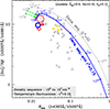 |
Fig. 8. Dereddened NLR ratios of [O III]/Hβ versus ROIII for the same observational dataset as in Fig. 4. The gray dotted line consists of radiation pressure stratified ionization-bounded models with Uo = 0.1 assuming the Fg97 SED with Tcut = 106 K. The frontal density along the sequence varies from |


We evaluated the extra energy required to generate the temperature fluctuations and found that the integrated cooling rate of the plasma with t2 = 0.15 was 50% higher than when the equilibrium temperature Teq is assumed19, which is an uncomfortably large fraction. To confirm the hypothesis of small scale NLR temperature inhomogeneities would in any case require observations of the weak recombinations lines of O II as was achieved in PNe and H II regions. A possibility could be deep spectroscopy of the radially distant ENLR associated to radio-galaxies such as in Pks 2152-69 (Tadhunter et al. 1987) where the underlying stellar emission is weak and only a dust-reflected AGN continuum is present.
7.4. Non-Maxwellian energy distributions
Another possibility to reach higher ROIII values is to consider a κ-distribution of the electron kinetic energy rather than the standard Maxwell–Boltzmann (hereafter M-B) energy distribution. One advantage of this approach is that it does not require an additional heating mechanism as was the case with the temperature fluctuations considered in Sect. 7.3. What is needed, however, is a mechanism that could account for the distortion of the kinetic energies of the electrons.
7.4.1. Context of kappa versus M-B distributions
The assumption that the velocity distribution of the free electrons in gaseous nebulae are described by a M-B distribution is based on the electron thermalization timescale. It is usually assumed that free electrons share their energy with the neighbouring medium so rapidly that they become thermalized before they excite any emission line. This is assumed because the energy redistribution through elastic collisions of electrons occurs faster than any other process (e.g., Draine & Kreisch 2018). However, if energetic electrons are injected into the gas continually and sufficiently quickly that the particle distribution does not have time to relax to a classical equilibrium distribution, then κ-distributions may arise. Although κ-distributions were initially criticized for lacking a theoretical justification, Tsallis et al. (1996) showed how these distributions can appear using entropy considerations and it has also been shown that they can arise from Tsallis’s non-extensive statistical mechanics (e.g., Leubner 2002; Livadiotis & McComas 2009). For a review on κ-distributions and on the mechanisms proposed to generate them in space plasmas, see Pierrard & Lazar (2010).
Nicholls et al. (2012) proposed various mechanisms that could induce and maintain a κ-distribution within photoionized regions. These include the injection of a population of energetic electrons by acceleration mechanisms such as magnetic reconnection and development of inertial Alfvén waves, shocks, and the injection of high-energy electrons through the photoionization process. Energetic electrons can be produced by the photoionization of dust (Dopita & Sutherland 2000), and X-ray or EUV photoionization (Shull & van Steenberg 1985; Petrini & da Silva 1997). Active galactic nuclei are regions where shocks, winds, and turbulence are known to be present (e.g., Baring 1991; Humphrey et al. 2008, 2010; Zhang et al. 2013; Silva et al. 2018), and these processes may also be sufficient to accelerate particles and generate a κ-distribution of electron energies. Several other processes, which are plausibly associated with AGN activity, may also be responsible for deviations from equilibrium, such as ionization by cosmic rays (Giammanco & Beckman 2005), and dissipative turbulence internal to the gas clouds (Mignoli et al. 2019).
7.4.2. Calculations assuming a κ-distribution
Electron κ-distributions have been directly measured in several solar system plasmas. They are present in the solar wind (e.g., Gloeckler et al. 1992; Maksimovic et al. 1997), in the outer heliosphere and the inner heliosleath (e.g., Decker & Krimigis 2003; Heerikhuisen et al. 2008), in planetary magnetospheres, including magnetosheath (e.g., Gloeckler & Hamilton 1987; Krimigis et al. 1983, 1986; Olbert 1968), and in magnetospheres of planetary moons (e.g., Jurac et al. 2002; Moncuquet et al. 2002).
Although it is apparent that κ-distributions are prevalent in solar system plasmas, but not until recent years has the possibility of κ-distributions in extrasolar gaseous nebulae been significantly explored. This possibility was investigated by Nicholls et al. (2012, hereafter Ni12), Binette et al. (2012) and Dopita et al. (2013) in the context of stellar-ionized gas. Morais et al. (2021) have recently compared photoionization models assuming a κ-distribution with the observed line ratios from a sample of 143 Type 2 AGNs. They found that for 98 objects, κ-distributions provide a better fit than M-B distributions.
In order to calculate the impact of a κ-distribution on our photoionization models, we used the analytical treatment developed by Ni12 and subsequently implemented in MAPPINGS I (see Binette et al. 2012 for details). Apart from taking into account the increased excitation rates of the atomic levels and the recombination rates of ionized species, MAPPINGS I also calculates the enhancement of collisional ionization that can result from κ-distributions.
Using the same metallicity as in previous models, we calculated a density sequence of ionization-bounded photoionization calculations assuming Uo = 0.1 and the thermal distribution of Fg97 with Tcut = 106 K as ionizing continuum. The density sequence calculations assuming κ = 7 for the electron velocity distribution (see Eq. (1) in Ni12) is represented by the black solid line in Fig. 9 while the gray dotted line corresponds to the same density sequence of M-B ionization-bounded models from Fig. 7 (i.e., κ = ∞). In both sequences the clouds internal density is stratified due to the progressive absorption of the ionizing continuum (see Sect. 7.2.1).
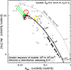 |
Fig. 9. Dereddened NLR ratios of [O III]/Hβ versus ROIII for the same observational dataset as in Fig. 4. The gray dotted line consists of radiation pressure stratified ionization-bounded models with Uo = 0.1 assuming the Fg97 SED with Tcut = 106 K. The frontal density along the sequence varies from |

The three light-green dashed arrows in Fig. 9 illustrate the change in line ratios for specific models of the M-B sequence (gray dotted line) when one assumes a κ-distribution with κ = 7. The frontal densities of these models correspond to  , 103.0 and 103.5 cm−3, respectively. They result in an [Ar IV] (λ4711Å/λ4740Å) line ratio of 1.13, 0.87 and 0.54, respectively, which are representative of the observed ratios among the S7 Seyfert 2s (Col. 9 in Table 2).
Owing to radiation pressure, the mean densities of the zones which emit the [Ar IV] lines is  . Interestingly, even though the integrated H Balmer line luminosities are not affected by κ (as they only depend on the flux of impinging ionizing photons ϕ0) the integrated columns of ionized H+ in the three models with κ = 7 turned out 25% lower because the H+ recombination rates are 25% higher than with the M-B models.
To conclude, the models with κ ≃ 7 and densities  can reproduce the observed [Ar IV] and ROIII ratios. Also, owing to the higher cooling efficiency of the models that assume κ-distributions, the average plasma temperature for the
  model is actually lower, by about 1100 K, than the same model assuming a M-B distribution (i.e., κ = ∞). Morais et al. (2021) have performed a more detailed comparison of the M-B distribution models with those that assume a κ-distribution. Their analysis consisted in exploring different values for the ionization parameter, the continuum spectral index, the plasma density and its metallicity. For a majority of objects from their 143 Type II AGNs sample, their analysis favored the κ-distribution approach.
We consider that κ-distributions have the potential of resolving the TE problem. We must emphasize, however, that if κ-distributions applied to the NLR, the observed ROIII ratio can no more serve as temperature indicator. The three κ = 7 models with densities similar to those inferred from the S7 sample show an average plasma temperature of ≈10 300 rather than the previously inferred value of 13 000 K (Sect. 4) based on a standard M-B distribution.
8. Summary and conclusions
Following a brief review of previous studies about the densities encountered in both the NLR and ENLR emission regions (Sect. 2), we are proposing the utilization of the [Ar IV] (λ4711Å/λ4740Å) doublet ratio to evaluate to what extent the temperatures derived from the [O III] (λ4363Å/λ5007Å) ratios of the NLR are affected by collisional deexcitation. Our Seyfert 2 sample was originally extracted from the final data release (Dopita et al. 2015; Thomas et al. 2017) of the Siding Spring Southern Seyfert Spectroscopic Snapshot Survey. Since our analysis centers on measurements of very weak lines, we found necessary to repeat the line extraction and line fitting procedure to ensure that the stellar spectral features surrounding the [Ar IV] λλ4711,40Å lines were properly subtracted and also to determine which aperture provided the best S/N ratio for the extracted lines (i.e., 1″ or 4″).
We extracted reliable NLR measurements of the [Ar IV] doublet in 16 high excitation Seyfert 2s of the S7 survey. The [Ar IV] λ4711Å line fluxes were subsequently corrected for blending due to the weaker He Iλ4713Å and [Ne IV] λλ4715Å lines. Among our sample, 13 Seyfert 2s cluster at a similar ROIII ratio of 0.0146 ± 0.0020 while three objects labeled outliers show significantly higher values (> 0.03). The plasma densities inferred from the [Ar IV] doublet for the 13 Seyfert 2s group span over the range 2.4103 to 5.4104 cm−3 in the single density case (Table 2). The average temperature derived from ROIII for the 13 objects is 13 000 ± 703 K. Alternatively, when for each object a decreasing power-law density distribution is assumed that extends up to a cut-off density ncut, the averaged values of the plasma densities that we infer for each object all turn out lower than 6.7 × 104 cm−3 (Table 3). The average temperature derived from ROIII in this case is 12 961 ± 711 K, which is similar to the single density case.
Assuming the thermal SED of Fg97 with Tcut = 106.0 K (Fig. 5) and a gas metallicity of 2.5 Z⊙, which is within the range expected for galactic nuclei of spiral galaxies, the photoionization models assuming low densities calculated with MAPPINGS I could not reproduce the observed ROIII ratios, which we labeled the TE problem. We subsequently addressed this issue by exploring alternative mechanisms that could account for the observed ROIII ratios while assuming plasma densities that encompassed those inferred from the [Ar IV] doublet. For instance, in order to reproduce an ROIII ratio close to the observed mean value of 0.015, we considered four mechanisms as follows. In Sect. 7.1, we explored the possibility of a double-bump SED where the second peak occurs near 200 eV. One advantage of this method is that it can also account for the soft X-ray excess observed by the XMM-Newton satellite. In Sect. 7.2, we explored the possibility of high ionization matter-bounded clouds. Although a promising solution, the calculated He II/Hβ ratio was much higher than observed, by a factor 2.4. In Sect. 7.3, following the approach of BL00, we hypothesized the existence of significant temperature inhomogeneities within the NLR clouds. To confirm this proposition would require the detection of the O II V1 multiplet. Finally, in Sect. 7.4 we considered the possibility of a κ electron energy distribution, with κ = 7. One advantage of this approach was that it did not require an additional heating mechanism although the immediate cause of the distortion of the M-B electron velocities remained indeterminate. We note that if the κ-distribution mechanism was confirmed, the ROIII ratio would no more serve as a direct temperature diagnostics.
Independently of the origin of the TE problem, the fact remains that Type I and Type II AGNs reveal significant differences insofar as the optical [O III] lines are concerned. There is a clear demarcation in the [O III] (λ4363Å/λ5007Å) versus ROIII diagram of the Seyfert 2’s from the S7 survey with respect to quasars and narrow-line Seyfert 1 galaxies. The most likely interpretation is that collisional deexcitation is significantly affecting the line emission of Type I nuclei where we have full view of the inner NLR and possibly systems at an intermediate orientation as might be the case for the few outliers of the S7 survey. The classical AGN unified model, which proposes that the NLR should be isotropic, is clearly an incomplete picture.
The term “quasar” is used to refer to Type I AGNs.
From level 1D2 to levels 3P1 and 3P2.
In accordance to the definition of critical density from Osterbrock (1989).
Currently available at https://docs.datacentral.org.au/s7/
The appended + symbol denotes the presence of line blending.
NGC4 24, NGC 1052, ESO 362-G18, MCG-01-24-012, NGC 3281, NGC3 783, NGC 3831, NGC 4593, ESO 339-G11, NGC 6860, IC 5063 and NGC 7590.
The S7 and BVM samples have one object in common: Mrk 573.
To determine the α25 − 60 index, the fluxes were taken from Meléndez et al. (2008b) and from NED (Helou & Madore 1988).
The algorithm OSALD is a routine of the code MAPPINGS I. Both software share the same atomic database.
Defined as the line emission coefficient times the electronic density.
Ω(n) = A(n)/4πr2 where A is the area of a shell of density n exposed to the ionizing source at a distance r. For definiteness we set the electron density equal to that of H: n = ne = nH.
As measured using the “broad/intermediate” line profile fits, see nomenclature of NLR profiles defined by Holt et al. (2008).
It included one object confirmed as Type 1.8 and another as Type 1.9.
To deblend the [Ar IV] doublet ratio of Mrk 573, we used the He I (λ3889Å/λ4740Å) ratio since neither the He Iλ5876Å nor the λ4471Å line were reported.
The density at the illuminated face of the photoionized gas shell.
In BK23, this value was erroneously qualified as equivalent to the αUV assumed by Ri14 and Fg97, which is αFUV = −0.3.
The O II V1 multiplet consists of eight recombination emission lines at the wavelengths of 4651, 4673, 4638, 4462, 4696, 4642, 4676 and 4649 Å, respectively. The integrated luminosity of the whole multiplet is insensitive to the electronic density (Peimbert et al. 2014; Storey et al. 2014).
This corresponds to a Γheat value of 0.5 as defined by Eq. (12) of BL00.
Acknowledgments
The S7 survey was made possible by the support of the Australian Research Council through the Discovery Project DP160103631. O.L.D. is grateful to Fundacão de Amparo à Pesquisa do Estado de São Paulo (FAPESP) and to Conselho Nacional de Desenvolvimento Científico e Tecnológico (CNPq). R.A.R. acknowledges financial support from Conselho Nacional de Desenvolvimento Científico e Tecnológico and Fundação de Amparo à pesquisa do Estado do Rio Grande do Sul. M.V.M. acknowledges support from grant PID2021-124665NB-I00 by the Spanish Ministry of Science and Innovation/State Agency of Research MCIN/AEI/10.13039/501100011033 and by “ERDF A way of making Europe”. C.M. acknowledges the support of UNAM/DGAPA/PAPIIT grants IN101220 and IG101223.
References
- Allen, J. T., Hewett, P. C., Richardson, C. T., Ferland, G. J., & Baldwin, J. A. 2013, MNRAS, 430, 3510 [NASA ADS] [CrossRef] [Google Scholar]
- Alloin, D., Bica, E., Bonatto, C., & Prugniel, P. 1992, A&A, 266, 117 [NASA ADS] [Google Scholar]
- Antonucci, R. 1993, ARA&A, 31, 473 [Google Scholar]
- Asplund, M., Grevesse, N., & Sauval, J. A. 2006, Nucl. Phys. A, 777, 1 [CrossRef] [Google Scholar]
- Baldwin, J., Ferland, G., Korista, K., & Verner, D. 1995, ApJ, 455, L119 [NASA ADS] [Google Scholar]
- Ballero, S. K., Matteucci, F., Ciotti, L., Calura, F., & Padovani, P. 2008, A&A, 478, 335 [NASA ADS] [CrossRef] [EDP Sciences] [Google Scholar]
- Baring, M. G. 1991, MNRAS, 253, 388 [CrossRef] [Google Scholar]
- Baron, D., & Netzer, H. 2019, MNRAS, 486, 4290 [Google Scholar]
- Baskin, A., & Laor, A. 2005, MNRAS, 358, 1043 [Google Scholar]
- Bennert, N., Jungwiert, B., Komossa, S., Haas, M., & Chini, R. 2006a, A&A, 459, 55 [NASA ADS] [CrossRef] [EDP Sciences] [Google Scholar]
- Bennert, N., Jungwiert, B., Komossa, S., Haas, M., & Chini, R. 2006b, A&A, 456, 953 [NASA ADS] [CrossRef] [EDP Sciences] [Google Scholar]
- Bennert, N., Jungwiert, B., Komossa, S., Haas, M., & Chini, R. 2006c, New Astron. Rev., 50, 708 [CrossRef] [Google Scholar]
- Binette, L. 1998, MNRAS, 294, L49 [NASA ADS] [CrossRef] [Google Scholar]
- Binette, L., & Luridiana, V. 2000, Rev. Mex. Astron. Astrofis., 36, 43 [NASA ADS] [Google Scholar]
- Binette, L., Dopita, M. A., & Tuohy, I. R. 1985, ApJ, 297, 476 [NASA ADS] [CrossRef] [Google Scholar]
- Binette, L., Wilson, A. S., & Storchi-Bergmann, T. 1996, A&A, 312, 365 [NASA ADS] [Google Scholar]
- Binette, L., Wilson, A. S., Raga, A., & Storchi-Bergmann, T. 1997, A&A, 327, 909 [NASA ADS] [Google Scholar]
- Binette, L., Magris C., G., Krongold, Y., et al. 2005, ApJ, 631, 661 [NASA ADS] [CrossRef] [Google Scholar]
- Binette, L., Matadamas, R., Hägele, G. F., et al. 2012, A&A, 547, A29 [NASA ADS] [CrossRef] [EDP Sciences] [Google Scholar]
- Binette, L., Villar Martín, M., Magris, C. G., et al. 2022, Rev. Mex. Astron. Astrofis., 58, 133 [Google Scholar]
- Binette, L., Krongold, Y., Haro-Corzo, S. A. R., Humphrey, A., & Morais, S. G. 2023, Rev. Mex. Astron. Astrofis., 59, 113 [Google Scholar]
- Boroson, T. A., & Green, R. F. 1992, ApJS, 80, 109 [Google Scholar]
- Cameron, M., Storey, J. W. V., Rotaciuc, V., et al. 1993, ApJ, 419, 136 [NASA ADS] [CrossRef] [Google Scholar]
- Cappellari, M. 2017, MNRAS, 466, 798 [Google Scholar]
- Cappellari, M., & Emsellem, E. 2004, PASP, 116, 138 [Google Scholar]
- Cerqueira-Campos, F. C., Rodríguez-Ardila, A., Riffel, R., et al. 2021, MNRAS, 500, 2666 [Google Scholar]
- Cheng, H., Yuan, W., Liu, H.-Y., et al. 2019, MNRAS, 487, 3884 [NASA ADS] [CrossRef] [Google Scholar]
- Congiu, E., Contini, M., Ciroi, S., et al. 2017, MNRAS, 471, 562 [Google Scholar]
- Croton, D. J., Springel, V., White, S. D. M., et al. 2006, MNRAS, 365, 11 [Google Scholar]
- Davies, R., Baron, D., Shimizu, T., et al. 2020, MNRAS, 498, 4150 [Google Scholar]
- Decker, R. B., & Krimigis, S. M. 2003, Adv. Space Res., 32, 597 [NASA ADS] [CrossRef] [Google Scholar]
- Done, C., Davis, S. W., Jin, C., Blaes, O., & Ward, M. 2012, MNRAS, 420, 1848 [Google Scholar]
- Dopita, M. A., & Sutherland, R. S. 2000, ApJ, 539, 742 [NASA ADS] [CrossRef] [Google Scholar]
- Dopita, M. A., Groves, B. A., Sutherland, R. S., Binette, L., & Cecil, G. 2002, ApJ, 572, 753 [NASA ADS] [CrossRef] [Google Scholar]
- Dopita, M., Rhee, J., Farage, C., et al. 2010, Ap&SS, 327, 245 [Google Scholar]
- Dopita, M. A., Sutherland, R. S., Nicholls, D. C., Kewley, L. J., & Vogt, F. P. A. 2013, ApJS, 208, 10 [NASA ADS] [CrossRef] [Google Scholar]
- Dopita, M. A., Scharwächter, J., Shastri, P., et al. 2014, A&A, 566, A41 [NASA ADS] [CrossRef] [EDP Sciences] [Google Scholar]
- Dopita, M. A., Shastri, P., Davies, R., et al. 2015, ApJS, 217, 12 [NASA ADS] [CrossRef] [Google Scholar]
- Dors, O. L., Cardaci, M. V., Hägele, G. F., et al. 2015, MNRAS, 453, 4102 [Google Scholar]
- Draine, B. T., & Kreisch, C. D. 2018, ApJ, 862, 30 [NASA ADS] [CrossRef] [Google Scholar]
- Durret, F., & Bergeron, J. 1986, A&A, 156, 51 [NASA ADS] [Google Scholar]
- Esteban, C., Peimbert, M., Torres-Peimbert, S., & Escalante, V. 1998, MNRAS, 295, 401 [NASA ADS] [CrossRef] [Google Scholar]
- Ferguson, J. W., Korista, K. T., Baldwin, J. A., & Ferland, G. J. 1997, ApJ, 487, 122 [NASA ADS] [CrossRef] [Google Scholar]
- Fitzpatrick, E. L. 1999, PASP, 111, 63 [Google Scholar]
- Fitzpatrick, E. L., & Massa, D. 2007, ApJ, 663, 320 [Google Scholar]
- Freitas, I. C., Riffel, R. A., Storchi-Bergmann, T., et al. 2018, MNRAS, 476, 2760 [Google Scholar]
- Froese Fischer, C., & Tachiev, G. 2004, At. Data Nucl. Data Tables, 87, 1 [NASA ADS] [CrossRef] [Google Scholar]
- García-Rojas, J., Madonna, S., Luridiana, V., et al. 2015, MNRAS, 452, 2606 [CrossRef] [Google Scholar]
- Giammanco, C., & Beckman, J. E. 2005, A&A, 437, L11 [NASA ADS] [CrossRef] [EDP Sciences] [Google Scholar]
- Gloeckler, G., & Hamilton, D. C. 1987, Phys. Scr. Vol. T, 18, 73 [NASA ADS] [CrossRef] [Google Scholar]
- Gloeckler, G., Geiss, J., Balsiger, H., et al. 1992, A&AS, 92, 267 [NASA ADS] [Google Scholar]
- González Delgado, R. M., Cerviño, M., Martins, L. P., Leitherer, C., & Hauschildt, P. H. 2005, MNRAS, 357, 945 [Google Scholar]
- Haro-Corzo, S. A. R., Binette, L., Krongold, Y., et al. 2007, ApJ, 662, 145 [NASA ADS] [CrossRef] [Google Scholar]
- Heerikhuisen, J., Pogorelov, N. V., Florinski, V., Zank, G. P., & le Roux, J. A. 2008, ApJ, 682, 679 [NASA ADS] [CrossRef] [Google Scholar]
- Helou, G., & Madore, B. 1988, ESO Conf. Workshop Proc., 28, 335 [NASA ADS] [Google Scholar]
- Ho, I. T., Medling, A. M., Groves, B., et al. 2016, Ap&SS, 361, 280 [CrossRef] [Google Scholar]
- Holden, L. R., Tadhunter, C. N., Morganti, R., & Oosterloo, T. 2023, MNRAS, 520, 1848 [NASA ADS] [CrossRef] [Google Scholar]
- Holt, J., Tadhunter, C. N., & Morganti, R. 2008, MNRAS, 387, 639 [NASA ADS] [CrossRef] [Google Scholar]
- Holt, J., Tadhunter, C. N., Morganti, R., & Emonts, B. H. C. 2011, MNRAS, 410, 1527 [NASA ADS] [Google Scholar]
- Humphrey, A., Villar-Martín, M., Vernet, J., et al. 2008, MNRAS, 383, 11 [NASA ADS] [CrossRef] [Google Scholar]
- Humphrey, A., Villar-Martín, M., Sánchez, S. F., et al. 2010, MNRAS, 408, L1 [NASA ADS] [CrossRef] [Google Scholar]
- Jackson, N., & Browne, I. W. A. 1991, MNRAS, 250, 422 [NASA ADS] [CrossRef] [Google Scholar]
- Jurac, S., McGrath, M. A., Johnson, R. E., et al. 2002, Geophys. Res. Lett., 29, 2172 [NASA ADS] [Google Scholar]
- Kakkad, D., Groves, B., Dopita, M., et al. 2018, A&A, 618, A6 [NASA ADS] [CrossRef] [EDP Sciences] [Google Scholar]
- Keel, W. C., de Grijp, M. H. K., Miley, G. K., & Zheng, W. 1994, A&A, 283, 791 [Google Scholar]
- Kewley, L. J., Nicholls, D. C., Sutherland, R., et al. 2019, ApJ, 880, 16 [Google Scholar]
- Komossa, S., & Schulz, H. 1997, A&A, 323, 31 [NASA ADS] [Google Scholar]
- Korista, K., Baldwin, J., Ferland, G., & Verner, D. 1997, ApJS, 108, 401 [NASA ADS] [CrossRef] [Google Scholar]
- Koski, A. T. 1978, ApJ, 223, 56 [NASA ADS] [CrossRef] [Google Scholar]
- Kraemer, S. B., Ruiz, J. R., & Crenshaw, D. M. 1998, ApJ, 508, 232 [CrossRef] [Google Scholar]
- Kraemer, S. B., Schmitt, H. R., Crenshaw, D. M., et al. 2011, ApJ, 727, 130 [NASA ADS] [CrossRef] [Google Scholar]
- Krimigis, S. M., Carbary, J. F., Keath, E. P., et al. 1983, J. Geophys. Res., 88, 8871 [CrossRef] [Google Scholar]
- Krimigis, S. M., Armstrong, T. P., Axford, W. I., et al. 1986, Science, 233, 97 [NASA ADS] [CrossRef] [Google Scholar]
- Lawrence, A. 2012, MNRAS, 423, 451 [NASA ADS] [CrossRef] [Google Scholar]
- Leubner, M. P. 2002, Ap&SS, 282, 573 [NASA ADS] [CrossRef] [Google Scholar]
- Livadiotis, G., & McComas, D. J. 2009, J. Geophys. Res. Space Phys., 114, A11105 [NASA ADS] [CrossRef] [Google Scholar]
- Luridiana, V., Morisset, C., & Shaw, R. A. 2015, A&A, 573, A42 [NASA ADS] [CrossRef] [EDP Sciences] [Google Scholar]
- Maksimovic, M., Pierrard, V., & Lemaire, J. F. 1997, A&A, 324, 725 [NASA ADS] [Google Scholar]
- Mazzalay, X., & Rodríguez-Ardila, A. 2007, A&A, 463, 445 [NASA ADS] [CrossRef] [EDP Sciences] [Google Scholar]
- Mazzalay, X., Rodríguez-Ardila, A., & Komossa, S. 2010, MNRAS, 405, 1315 [NASA ADS] [Google Scholar]
- Meléndez, M., Kraemer, S. B., Armentrout, B. K., et al. 2008a, ApJ, 682, 94 [Google Scholar]
- Meléndez, M., Kraemer, S. B., Schmitt, H. R., et al. 2008b, ApJ, 689, 95 [Google Scholar]
- Méndez-Delgado, J. E., Esteban, C., García-Rojas, J., Kreckel, K., & Peimbert, M. 2023, Nature, 618, 249 [CrossRef] [Google Scholar]
- Mignoli, M., Feltre, A., Bongiorno, A., et al. 2019, A&A, 626, A9 [NASA ADS] [CrossRef] [EDP Sciences] [Google Scholar]
- Moncuquet, M., Bagenal, F., & Meyer-Vernet, N. 2002, J. Geophys. Res. Space Phys., 107, 1260 [NASA ADS] [CrossRef] [Google Scholar]
- Morais, S. G., Humphrey, A., Villar Martín, M., Binette, L., & Silva, M. 2021, MNRAS, 506, 1389 [CrossRef] [Google Scholar]
- Moran, E. C., Barth, A. J., Kay, L. E., & Filippenko, A. V. 2000, ApJ, 540, L73 [NASA ADS] [CrossRef] [Google Scholar]
- Morganti, R., Robinson, A., Fosbury, R. A. E., et al. 1991, MNRAS, 249, 91 [NASA ADS] [Google Scholar]
- Morganti, R., Oosterloo, T., Oonk, J. B. R., Frieswijk, W., & Tadhunter, C. 2015, A&A, 580, A1 [NASA ADS] [CrossRef] [EDP Sciences] [Google Scholar]
- Morisset, C., Luridiana, V., García-Rojas, J., et al. 2020, Atoms, 8, 66 [NASA ADS] [CrossRef] [Google Scholar]
- Mulchaey, J. S., Koratkar, A., Ward, M. J., et al. 1994, ApJ, 436, 586 [NASA ADS] [CrossRef] [Google Scholar]
- Mullaney, J. R., Alexander, D. M., Fine, S., et al. 2013, MNRAS, 433, 622 [Google Scholar]
- Nagao, T., Murayama, T., & Taniguchi, Y. 2001, ApJ, 549, 155 [NASA ADS] [CrossRef] [Google Scholar]
- Nagao, T., Murayama, T., Shioya, Y., & Taniguchi, Y. 2002, ApJ, 575, 721 [NASA ADS] [CrossRef] [Google Scholar]
- Nesvadba, N. P. H., Lehnert, M. D., De Breuck, C., Gilbert, A. M., & van Breugel, W. 2008, A&A, 491, 407 [NASA ADS] [CrossRef] [EDP Sciences] [Google Scholar]
- Netzer, H., Mainieri, V., Rosati, P., & Trakhtenbrot, B. 2006, A&A, 453, 525 [NASA ADS] [CrossRef] [EDP Sciences] [Google Scholar]
- Nicholls, D. C., Dopita, M. A., & Sutherland, R. S. 2012, ApJ, 752, 148 [NASA ADS] [CrossRef] [Google Scholar]
- Nicholls, D. C., Sutherland, R. S., Dopita, M. A., Kewley, L. J., & Groves, B. A. 2017, MNRAS, 466, 4403 [Google Scholar]
- Olbert, S. 1968, Astrophys. Space Sci. Lib., 10, 641 [NASA ADS] [CrossRef] [Google Scholar]
- Osterbrock, D. E. 1989, Astrophysics of Gaseous Nebulae and Active Galactic Nuclei (University Science Books) [Google Scholar]
- Peimbert, M. 1967, ApJ, 150, 825 [NASA ADS] [CrossRef] [Google Scholar]
- Peimbert, M. 1995, in The Analysis of Emission Lines: A Meeting in Honor of the 70th Birthdays of D. E. Osterbrock& M. J. Seaton, eds. R. Williams, & M. Livio (Cambridge University Press), 165 [Google Scholar]
- Peimbert, M., Luridiana, V., & Torres-Peimbert, S. 1995, Rev. Mex. Astron. Astrofis., 31, 147 [NASA ADS] [Google Scholar]
- Peimbert, A., Peimbert, M., Delgado-Inglada, G., García-Rojas, J., & Peña, M. 2014, Rev. Mex. Astron. Astrofis., 50, 329 [Google Scholar]
- Pequignot, D., Petitjean, P., & Boisson, C. 1991, A&A, 251, 680 [NASA ADS] [Google Scholar]
- Petrini, D., & da Silva, E. P. 1997, A&A, 317, 262 [NASA ADS] [Google Scholar]
- Piconcelli, E., Jimenez-Bailón, E., Guainazzi, M., et al. 2005, A&A, 432, 15 [NASA ADS] [CrossRef] [EDP Sciences] [Google Scholar]
- Pierrard, V., & Lazar, M. 2010, Sol. Phys., 267, 153 [NASA ADS] [CrossRef] [Google Scholar]
- Planck Collaboration VI. 2021, A&A, 652, C4 [NASA ADS] [CrossRef] [EDP Sciences] [Google Scholar]
- Porter, R. L., Ferland, G. J., Storey, P. J., & Detisch, M. J. 2013, MNRAS, 433, L89 [NASA ADS] [CrossRef] [Google Scholar]
- Pringle, J. E. 1981, ARA&A, 19, 137 [NASA ADS] [CrossRef] [Google Scholar]
- Ramsbottom, C. A., Bell, K. L., & Keenan, F. P. 1997, MNRAS, 284, 754 [NASA ADS] [Google Scholar]
- Revalski, M., Crenshaw, D. M., Kraemer, S. B., et al. 2018, ApJ, 856, 46 [NASA ADS] [CrossRef] [Google Scholar]
- Revalski, M., Meena, B., Martinez, F., et al. 2021, ApJ, 910, 139 [NASA ADS] [CrossRef] [Google Scholar]
- Revalski, M., Crenshaw, D. M., Rafelski, M., et al. 2022, ApJ, 930, 14 [NASA ADS] [CrossRef] [Google Scholar]
- Rhee, J. H., & Larkin, J. E. 2005, ApJ, 620, 151 [CrossRef] [Google Scholar]
- Richardson, C. T., Allen, J. T., Baldwin, J. A., Hewett, P. C., & Ferland, G. J. 2014, MNRAS, 437, 2376 [NASA ADS] [CrossRef] [Google Scholar]
- Rola, C., & Stasińska, G. 1994, A&A, 282, 199 [Google Scholar]
- Rose, M., Tadhunter, C., Ramos Almeida, C., et al. 2018, MNRAS, 474, 128 [Google Scholar]
- Ross, R. R., & Fabian, A. C. 2005, MNRAS, 358, 211 [CrossRef] [Google Scholar]
- Rynkun, P., Gaigalas, G., & Jönsson, P. 2019, A&A, 623, A155 [NASA ADS] [CrossRef] [EDP Sciences] [Google Scholar]
- Santoro, F., Rose, M., Morganti, R., et al. 2018, A&A, 617, A139 [NASA ADS] [CrossRef] [EDP Sciences] [Google Scholar]
- Schlafly, E. F., & Finkbeiner, D. P. 2011, ApJ, 737, 103 [Google Scholar]
- Scott, J. E., Kriss, G. A., Brotherton, M., et al. 2004, ApJ, 615, 135 [NASA ADS] [CrossRef] [Google Scholar]
- Shakura, N. I., & Sunyaev, R. A. 1973, A&A, 500, 33 [NASA ADS] [Google Scholar]
- Shang, Z., Brotherton, M. S., Green, R. F., et al. 2005, ApJ, 619, 41 [NASA ADS] [CrossRef] [Google Scholar]
- Shull, J. M., & van Steenberg, M. E. 1985, ApJ, 298, 268 [NASA ADS] [CrossRef] [Google Scholar]
- Silva, M., Humphrey, A., Lagos, P., et al. 2018, MNRAS, 474, 3649 [NASA ADS] [CrossRef] [Google Scholar]
- Skrutskie, M. F., Cutri, R. M., Stiening, R., et al. 2006, AJ, 131, 1163 [NASA ADS] [CrossRef] [Google Scholar]
- Spence, R. A. W., Tadhunter, C. N., Rose, M., & Rodríguez Zaurín, J. 2018, MNRAS, 478, 2438 [NASA ADS] [CrossRef] [Google Scholar]
- Stasińska, G. 1984, A&A, 135, 341 [NASA ADS] [Google Scholar]
- Storchi-Bergmann, T., & Pastoriza, M. G. 1990, PASP, 102, 1359 [NASA ADS] [CrossRef] [Google Scholar]
- Storchi-Bergmann, T., Wilson, A. S., Mulchaey, J. S., & Binette, L. 1996, A&A, 312, 357 [NASA ADS] [Google Scholar]
- Storchi-Bergmann, T., Fernandes, R. C., & Schmitt, H. R. 1998, ApJ, 501, 94 [NASA ADS] [CrossRef] [Google Scholar]
- Storey, P. J., & Zeippen, C. J. 2000, MNRAS, 312, 813 [NASA ADS] [CrossRef] [Google Scholar]
- Storey, P. J., Sochi, T., & Badnell, N. R. 2014, MNRAS, 441, 3028 [CrossRef] [Google Scholar]
- Sutherland, R. S., Bicknell, G. V., & Dopita, M. A. 2003, ApJ, 591, 238 [NASA ADS] [CrossRef] [Google Scholar]
- Tadhunter, C. N., Fosbury, R. A. E., Binette, L., Danziger, I. J., & Robinson, A. 1987, Nature, 325, 504 [NASA ADS] [CrossRef] [Google Scholar]
- Tadhunter, C. N., Metz, S., & Robinson, A. 1994, MNRAS, 268, 989 [NASA ADS] [CrossRef] [Google Scholar]
- Telfer, R. C., Zheng, W., Kriss, G. A., & Davidsen, A. F. 2002, ApJ, 565, 773 [NASA ADS] [CrossRef] [Google Scholar]
- Thomas, A. D., Dopita, M. A., Shastri, P., et al. 2017, ApJS, 232, 11 [NASA ADS] [CrossRef] [Google Scholar]
- Tran, H. D. 1995, ApJ, 440, 578 [NASA ADS] [CrossRef] [Google Scholar]
- Tran, H. D., Miller, J. S., & Kay, L. E. 1992, ApJ, 397, 452 [NASA ADS] [CrossRef] [Google Scholar]
- Tsallis, C., Levy, S. V. F., Souza, A. M. C., & Maynard, R. 1996, Phys. Rev. Lett., 77, 5442 [NASA ADS] [CrossRef] [Google Scholar]
- Vaona, L., Ciroi, S., Di Mille, F., et al. 2012, MNRAS, 427, 1266 [NASA ADS] [CrossRef] [Google Scholar]
- Véron-Cetty, M. P., & Véron, P. 2006, A&A, 455, 773 [Google Scholar]
- Véron-Cetty, M. P., & Véron, P. 2010, A&A, 518, A10 [Google Scholar]
- Viegas, S. M., & Prieto, M. A. 1992, MNRAS, 258, 483 [NASA ADS] [CrossRef] [Google Scholar]
- Villar-Martín, M., Humphrey, A., Martínez-Sansigre, A., et al. 2008, MNRAS, 390, 218 [CrossRef] [Google Scholar]
- Villar-Martín, M., Arribas, S., Emonts, B., et al. 2016, MNRAS, 460, 130 [Google Scholar]
- Wang, W., Liu, X. W., Zhang, Y., & Barlow, M. J. 2004, A&A, 427, 873 [NASA ADS] [CrossRef] [EDP Sciences] [Google Scholar]
- Winkel, N., Husemann, B., Davis, T. A., et al. 2022, A&A, 663, A104 [NASA ADS] [CrossRef] [EDP Sciences] [Google Scholar]
- Zhang, Z. T., Liang, Y. C., & Hammer, F. 2013, MNRAS, 430, 2605 [NASA ADS] [CrossRef] [Google Scholar]
- Zheng, W., Kriss, G. A., Telfer, R. C., Grimes, J. P., & Davidsen, A. F. 1997, ApJ, 475, 469 [NASA ADS] [CrossRef] [Google Scholar]
Appendix A: Plasma densities inferred from the [S II] doublet
Density diagnostics of the NLR typically rely on the [S II] (λ6716Å/λ6731Å) doublet ratio, which originates from the low ionization plasma. In Seyfert galaxies, the study of Bennert et al. (2006a,b) for instance reveals densities of the spatially resolved ENLR that are typically < 103 cm−3 and in most cases both the electron density and the ionization parameter appear to be decreasing with radius. More recently, Freitas et al. (2018), who used the Gemini multiObject Spectrograph Integral Field Unit (IFU) on the Gemini North Telescope, created two-dimensional electron density maps of the central part of five bright nearby Seyfert nuclei. These authors found electron density (ne) values, inferred from the [S II] (λ6716Å/λ6731Å) line ratio, ranging from ∼100 up to ∼2500 cm−3 along the AGN radius. The spatial resolution quoted in their Table 1 implies a seeing of ∼0.6″. A complementary work is that of Kakkad et al. (2018) who generated IFU electron density maps for an AGNs sample issued from the S7 survey which consisted of seven Seyfert 2 galaxies. The electron densities they inferred for the ENLR showed a positive gradient toward the nucleus, which was fitted with an exponential profile that initiated at a radius beyond the seeing size to avoid atmospheric blending. The density values they inferred covered the range of 50 to 2000 cm−3. As argued in App. A of BVM, for the ENLR these density values are probably not far-off from those characterizing the higher excitation lines such as [O III]. However, the situation is very different in the case of the unresolved NLR of Type I AGNs as shown by BL05 (see Fig. 4b) who presented clear evidence of strong collisional deexcitation of the ROIII ratio.
Appendix B: Correcting the [Ar IV] doublet from line blending
The observed [Ar IV]+ line at λ4711Åconsists of a blend with the much weaker He Iλ4713Å and [Ne IV] λλ4725Ålines. In order to properly determine the plasma densities, one must deblend the [Ar IV]+ (λλλ4711,13,15Å/λ4740Å) ratio of each object. As in BVM, the deblended [Ar IV] (λ4711Å/λ4740Å) ratio is obtained by subtracting, from the measured doublet [Ar IV]+ ratio, the fractional contribution from the He Iλ4713Å line ( ) and the [Ne IV] λλ4715Å line (
 ), that is:
![Mathematical equation: $$ \begin{aligned}[\mathrm{Ar}\,iv ] = (1 - f^{HeI}_{\rm blend} - f^{NeIV}_{\rm blend}) \times [\mathrm{Ar}\,iv ]{\tiny +} \end{aligned} $$](/articles/aa/full_html/2024/04/aa45754-22/aa45754-22-eq93.gif)
with each blending correction evaluated as follows.
B.1. Blending of the He Iλ4713Å line
One characteristic of ratios involving recombination lines of the same ion is their limited sensitivity to either temperature or density. A valid prediction of the He Iλ4713Å line intensity can therefore be derived from the measurement of the He I (λ5876Å line) (alternatively, one can use the He Iλ4471Å line). Our deblending procedure is as follows. First, we derive the Case B He I (λ4713Å/λ5876Å) ratio, which we label RHe, via interpolation of the emissivities from the supplemental Table of Porter et al. (2013). For a 104 cm−3 plasma at a temperature of 12 000 K, the RHe ratio turns out to be only 4.78% of He Iλ5876Å. Temperature variations of ±2000 K would cause a change in this ratio of  %, respectively, while adopting density values in the interval 102 to 105 cm−3 would result in RHe ratios between 0.0429 and 0.0489, respectively. Second, by defining RHe/Ar as the observed He I/[Ar IV] (λ5876Å/λ4740Å) ratio, the product (RHe × RHe/Ar) defines our estimate of
  , which is the contribution from He Iλ4713Å blending to the “measured” [Ar IV]+ doublet ratio. The
  values for the S7 survey assuming a single density are shown in Col. 6 of Table 2.
B.2. Blending of the [Ne IV] λλ4715Å line.
The [Ne IV] optical lines consist of a quadruplet at λ4714.36, λ4715.80, λ4724.15 and λ4726.62Å, respectively (García-Rojas et al. 2015). To simplify the notation, we refer to the quadruplet as consisting of two doublets: the observed [Ne IV] λλ4725Å doublet and the potentially blended [Ne IV] λλ4715Å doublet. At typical NLR densities and temperatures, the observed [Ne IV] λλ4725Å doublet turns out to be ≈35% brighter than the blended [Ne IV] λλ4715Å doublet. The dependence of this ratio on temperature and densities is relatively minor. Within the S7 survey, we could detect the λλ4715Å doublet only in a few objects. To correct the measured [Ar IV]+ ratio from [Ne IV] blending, we first calculate at the appropriate density and temperature the [Ne IV] (λλ4715Å/λλ4725Å) ratio, which we label RNe. By defining RNe/Ar as the observed [Ne IV]/[Ar IV] (λλ4725Å/λ4740Å) ratio, the product (RNe× RNe/Ar) defines our estimate of  , which is the contribution from [Ne IV] blending to the “measured” [Ar IV]+ doublet ratio.
Appendix C: Recent updates to the code MAPPINGS Ig
We incorporated the following recombination emission line processes to the version Ig of MAPPINGS I.
C.1. Emission resulting from recombination of N+2, O+3, O+2 and S+3 to metastable levels
Based on the work of Pequignot et al. (1991), the recombination rates from N+2, O+3 and O+2 to the corresponding metastable levels  and
and  of [N II] and [O III] and levels 2P and 2D of [O II], respectively, have been incorporated in the calculation of the corresponding emission line intensities. In the case of the
  level of [O III], we added the missing contribution from dielectronic recombination (Christophe Morisset, private communication). As for the S+2 and S+3 ions, we estimated their recombination rates to metastable levels by extrapolation from the O+2 and O+3 ions as follows: we assumed that the fraction, ξ, of the total recombination rate (
 or
or  ), which populates metastable levels of Sulfur is the same fraction as found for Oxygen. For instance, for a 10 000 K plasma this fraction,
  , in the case of level
  of O III (causing emission of the [O III] λ4363Å line), is 2.2% of
  .
.
All Tables
High excitation Seyfert 2s from the S7 survey with reliable measurements of the [Ar IV] doublet.
NLR temperatures derived using the reddening-corrected ratios for our sample extracted from the S7 survey.
All Figures
|
Fig. 1. Observed spectrum of Mrk 573 (black solid line). The LZIFU emission line fit (red) is superimposed to the dashed line which represents the stellar continuum fit. |
| In the text | |
|
Fig. 2. Spectra showing the [Ar IV] doublet lines of six Seyfert 2s (black solid line) from our sample after subtraction of the stellar and AGN continuum fit. From left to right: NGC 5643, Mrk 573, ESO 137-G34, NGC 3393, IC 2560 and Mrk 1210. The LZIFU emission line fit (magenta line) is superimposed to each spectrum. |
| In the text | |
|
Fig. 3. Pearson correlation coefficients for our sample of high excitation Seyfert 2s from the S7 survey. From bottom to top panel, the V band extinction in magnitudes AV and the extinction corrected values of observed [Ar IV]+ (λ4711Å+/λ4740Å), [O III] (λ5007Å/λ4861Å) and ROIII line ratios (Tables 1 and 2) versus the aperture D (in kpc) used to extract the spectra. The value of the Pearson correlation coefficient (P) is indicated in each panel. The red points identify the three outliers discussed in Sect. 3.5. |
| In the text | |
|
Fig. 4. Dereddened NLR ratios of [O III]/Hβ versus ROIII. Left panel a: blue dots represent the line ratios of 13 Seyfert 2s from the S7 survey sample which are listed in Table 1. Their average ROIII ratio is 0.0146 ± 0.0020, which is represented by the navy colored circle whose radius of 0.057 dex corresponds to the dispersion of the measurements. The yellow filled dots identifies the three outlier Seyfert 2s: ESO 138-G01, Mrk 1210 and NGC 4507 (labeled a, b, c in Table 1). Three complementary Seyfert 2 samples are represented by red open symbols: (1) the average of seven Seyfert 2s from Kos78 studied by BVM (large red circle), (2) the average of four Seyfert 2s from Be06b (small open circle with dispersion bars), (3) the high excitation Seyfert 2 subset a41 from Richardson et al. (2014; open red diamond). The light-gray open squares represent the ratios of Type I AGNs measured by BL05. Right panel b: a similar graph but with an expanded scale in order to cover the full range of ratios observed by BL05 among 30 quasars. The light-gray open triangles represent the four narrow-line Seyfert 1 galaxies observed by RA00. Both BL05 and RA00 subtracted the BLR profile component from Hβ before deriving the [O III]/Hβ ratio. The light-green filled symbols represent the spatially resolved ENLR measurements from three studies: (1) the average of two Seyfert 2s and two NLRGs (small light-green dot) from BWS, (2) the integrated long-slit spectrum of the Seyfert 2 IC 5063 from Be06b (pentagon), (3) the average of seven spatially resolved optical filaments of the radio-galaxy Centaurus A (light-green triangle) from Mo91. The blue segmented arrow at the top describes the effect of collisional deexcitation on the ROIII ratio for a 13 000 K isothermal plasma whose density is increased to successively larger values, from 102 to 106.5 cm−3. |
| In the text | |
|
Fig. 5. Ionizing SEDs in νFν units: (1) the SED adopted by Fg97 for their LOC calculations using Tcut = 106.0 K (black long-dash line), (2) the optimized SED of Ri14 with Tcut = 105.62 K (black dotted short-dash line), (3) the double-bump distribution La |
| In the text | |
|
Fig. 6. Dereddened NLR ratios of [O III]/Hβ versus ROIII for the same observational dataset as in Fig. 4. Two ionization parameter sequences of isochoric photoionization calculations with a frontal density of |
| In the text | |
|
Fig. 7. Dereddened NLR ratios of [O III]/Hβ versus ROIII for the same observational dataset as in Fig. 4. The blue solid line represent the sequence of MB models in which the frontal densities varied from |
| In the text | |
|
Fig. 8. Dereddened NLR ratios of [O III]/Hβ versus ROIII for the same observational dataset as in Fig. 4. The gray dotted line consists of radiation pressure stratified ionization-bounded models with Uo = 0.1 assuming the Fg97 SED with Tcut = 106 K. The frontal density along the sequence varies from |
| In the text | |
|
Fig. 9. Dereddened NLR ratios of [O III]/Hβ versus ROIII for the same observational dataset as in Fig. 4. The gray dotted line consists of radiation pressure stratified ionization-bounded models with Uo = 0.1 assuming the Fg97 SED with Tcut = 106 K. The frontal density along the sequence varies from |
| In the text | |
Current usage metrics show cumulative count of Article Views (full-text article views including HTML views, PDF and ePub downloads, according to the available data) and Abstracts Views on Vision4Press platform.
Data correspond to usage on the plateform after 2015. The current usage metrics is available 48-96 hours after online publication and is updated daily on week days.
Initial download of the metrics may take a while.