| Issue |
A&A
Volume 682, February 2024
|
|
|---|---|---|
| Article Number | L13 | |
| Number of page(s) | 8 | |
| Section | Letters to the Editor | |
| DOI | https://doi.org/10.1051/0004-6361/202348822 | |
| Published online | 09 February 2024 | |
Letter to the Editor
Study of the HCCNC and HNCCC isotopologs in TMC-1⋆
1
Dept. de Astrofísica Molecular, Instituto de Física Fundamental (IFF-CSIC), C/ Serrano 121, 28006 Madrid, Spain
e-mail: This email address is being protected from spambots. You need JavaScript enabled to view it.
; This email address is being protected from spambots. You need JavaScript enabled to view it.
2
Observatorio Astronómico Nacional (OAN, IGN), C/ Alfonso XII, 3, 28014 Madrid, Spain
3
Centro de Desarrollos Tecnológicos, Observatorio de Yebes (IGN), 19141 Yebes, Guadalajara, Spain
4
LERMA, Observatoire de Paris, PSL Research University, CNRS, Sorbonne Université, 92190 Meudon, France
Received:
1
December
2023
Accepted:
22
January
2024
Abstract
We present the detection of the three 13C isotopologs of HCCNC and HNCCC toward TMC-1 using the QUIJOTE line survey. In addition, the D species has also been detected for these two isomers of HCCCN, whereas the 15N isotopolog was only detected for HCCNC. Using high-J lines of HCCNC and HNCCC, we were able to derive very precise rotational temperatures, column densities, and subsequently the isotopic abundance ratios. We found that 12C/13C is ∼90 for the three possible substitutions in both isomers. These results are slightly different from what has been found for the most abundant isomer HCCCN, for which abundances of 105, 95, and 66 were found for each one of the three possible positions of 13C. The H/D abundance ratio was found to be 31 ± 4 for HCCNC and of 53 ± 6 for HNCCC. The latter is similar to the H/D abundance ratio derived for HCCCN (∼59). The 14N/15N isotopic abundance ratio in HCCNC is 243 ± 24.
Key words: astrochemistry / line: identification / molecular data / ISM: individual objects: TMC-1 / ISM: molecules
Based on observations carried out with the Yebes 40 m telescope (projects 19A003, 20A014, 20D023, 21A011, 21D005 and 23A024). The 40 m radio telescope at Yebes Observatory is operated by the Spanish Geographic Institute (IGN, Ministerio de Transportes, Movilidad y Agenda Urbana).
© The Authors 2024
 Open Access article, published by EDP Sciences, under the terms of the Creative Commons Attribution License (https://creativecommons.org/licenses/by/4.0), which permits unrestricted use, distribution, and reproduction in any medium, provided the original work is properly cited.
This article is published in open access under the Subscribe to Open model. This email address is being protected from spambots. You need JavaScript enabled to view it. to support open access publication.
1. Introduction
The ultra-sensitive line survey QUIJOTE1 performed with the Yebes 40 m radio telescope toward the prestellar cold core TMC-1 has enabled the unambiguous detection of near 50 molecules in the last three years (Cernicharo et al. 2021, 2023, and references therein). The sensitivity of QUIJOTE is unprecedented, opening up new issues concerning the interpretation of the forest of unknown lines present in sensitive spectral sweeps. In addition to the detection of new molecular species, which is the main goal of the survey, we have to deal with the contribution of all isotopologs of any molecule producing line intensities larger than 50 mK. Additionally, we must also account for the presence of low-lying bending vibrational modes of abundant species (see the case of the ν11 mode of C6H, Cernicharo et al. 2023). One of the advantages of QUIJOTE is that it can provide a detection (for all isotopologs) of a molecule whose emission is optically thin, thereby permitting a direct estimation of the isotopic abundances of species containing C, O, S, N, and H.
The study of isotopic abundances as a function of the distance to the galactic center allows to trace stellar nucleosynthesis and constrain the chemical enrichment in our galaxy (see, e.g., Yan et al. 2023). Moreover, molecules are known to experience isotopic fractionation and this can be used to track the chemical evolution of molecular clouds and the transfer of chemical content to planetary systems (Ceccarelli et al. 2014). In this work, we report the detection and spectroscopic characterization of all isotopologs of HCCNC, along with the first detection in space and first spectroscopic characterization, of the 13C isotopologs of HNCCC. The results presented here will allow us to improve the chemical models dealing with isotopic fractionation in molecular clouds (Roueff et al. 2015; Colzi et al. 2020; Loison et al. 2020; Sipilä et al. 2023). Although these models take into account 13C and 15N fractionation reactions with various degrees of approximation when including the dependence of the 13C position and adopted reactions, none of them deal with isotopic exchange reactions involving HNCCC and HCCNC.
2. Observations
The observational data used in this work are part of QUIJOTE (Cernicharo et al. 2021), a spectral line survey of TMC-1 in the Q-band carried out with the Yebes 40 m telescope at the position αJ2000 = 4h41m41.9s and δJ2000 = +25° 41′27.0″, corresponding to the cyanopolyyne peak (CP) in TMC-1. The receiver was built within the Nanocosmos project2 and consists of two cold high-electron mobility transistor amplifiers covering the 31.0–50.3 GHz band with horizontal and vertical polarizations. Receiver temperatures achieved in the 2019 and 2020 runs vary from 22 K at 32 GHz to 42 K at 50 GHz. Some power adaptation in the down-conversion chains have reduced the receiver temperatures during 2021 to 16 K at 32 GHz and 30 K at 50 GHz. The backends are 2 × 8 × 2.5 GHz fast Fourier transform spectrometers with a spectral resolution of 38 kHz, providing the whole coverage of the Q-band in both polarizations. A more detailed description of the system is given by Tercero et al. (2021).
The data of the QUIJOTE line survey presented here were gathered in several observing runs between November 2019 and July 2023. All observations are performed using frequency-switching observing mode with a frequency throw of 8 and 10 MHz. The total observing time on the source for data taken with frequency throws of 8 MHz and 10 MHz is 465 and 737 h, respectively. Hence, the total observing time on source is 1202 h. The measured sensitivity varies between 0.08 mK at 32 GHz and 0.2 mK at 49.5 GHz. The sensitivity of QUIJOTE is around 50 times better than that of previous line surveys in the Q band of TMC-1 (Kaifu et al. 2004). For each frequency throw, different local oscillator frequencies were used in order to remove possible side band effects in the down conversion chain. A detailed description of the QUIJOTE line survey is provided in Cernicharo et al. (2021). The data analysis procedure has been described by Cernicharo et al. (2022).
The main beam efficiency measured during our observations in 2022 varies from 0.66 at 32.4 GHz to 0.50 at 48.4 GHz (Tercero et al. 2021) and can be given across the Q-band by Beff = 0.797 exp[−(ν(GHz)/71.1)2]. The forward telescope efficiency is 0.97. The telescope beam size at half-power intensity is 54.4″ at 32.4 GHz and 36.4″ at 48.4 GHz.
Data for HCCNC and HNCCC in the millimeter domain have been taken with the IRAM 30 m telescope and consist of a 3 mm line survey that covers the full available band at the telescope, between 71.6 GHz and 117.6 GHz. The EMIR E0 receiver was connected to the Fourier transform spectrometers (FTS) in its narrow mode, which provide a spectral resolution of 49 kHz and a total bandwidth of 7.2 GHz per spectral setup. Observations were performed in several runs. Between January and May 2012, we completed the scan 82.5–117.6 GHz (Cernicharo et al. 2012). In August 2018, after the upgrade of the E090 receiver, we extended the survey down to 71.6 GHz. More recent high sensitivity observations in 2021 have been used to improve the signal to noise ratio (S/N) in several frequency windows (Agúndez et al. 2022; Cabezas et al. 2022). The final 3 mm line survey has a sensitivity of 2–10 mK. However, at some selected frequencies, the sensitivity is as low as 0.6 mK. All the observations were performed using the frequency-switching method with a frequency throw of 7.14 MHz. The IRAM 30 m beam varies between 34″ and 21″ at 72 GHz and 117 GHz, respectively, while the beam efficiency takes values of 0.83 and 0.78 at the same frequencies, following the relation: Beff = 0.871 exp[−(ν(GHz)/359)2]. The forward efficiency at 3 mm is 0.95.
The intensity scale utilized in this study is the antenna temperature ( ). The calibration was performed using two absorbers at different temperatures and the atmospheric transmission model ATM (Cernicharo 1985; Pardo et al. 2001). The absolute calibration uncertainty is 10%. However, the relative calibration between lines within the QUIJOTE survey is certainly better as all them are observed simultaneously. The data were analyzed with the GILDAS package3.
3. Results
Line identification in this work has been performed using the MADEX code (Cernicharo 2012), and the CDMS and JPL catalogues (Müller et al. 2005; Pickett et al. 1998). The references and laboratory data used by MADEX in its spectroscopic predictions are described below.
3.1. Spectroscopy of HCCNC
HCCNC was detected toward TMC-1 by Kawaguchi et al. (1992a). The dipole moment is 2.93 D (Krüger et al. 1991), which is lower than that of HCCCN. Guarnieri et al. (1992) observed rotational transitions of this species up to Ju = 33. Hence, the rotational and distortion constants have been well established. However, the hyperfine structure was observed only for the J = 1 − 0 line (Krüger et al. 1992). The hyperfine structure of the J = 4 − 3 and J = 5 − 4 lines was observed toward TMC-1 with a previous version of the QUIJOTE line survey (Cernicharo et al. 2020). We remeasured the frequencies of these lines with the present QUIJOTE data (see Table A.1). In addition, the J = 8 − 7 up to J = 11 − 10 lines of HCCNC were observed with the IRAM 30 m radio telescope. They are shown in Fig. A.1 and their line parameters are given in Table A.1. A fit to all the laboratory and space data was performed using the standard Hamiltonian of a linear molecule with a hyperfine structure. The results are given in Table 1. Therefore, the predictions for HCCNC, including the hyperfine structure, are reliable up to very high-J. In addition, DCCNC was also observed in the laboratory up to Ju = 51 (Huckauf et al. 1998). The situation was completely different for the 13C and 15N isotopologs, for which only the J = 1 − 0 transition has been observed in the laboratory (Krüger et al. 1992). All these isotopologs were observed and characterized spectroscopically by Cernicharo et al. (2020), who observed their J = 4 − 3 and J = 5 − 4 transitions toward TMC-1. The present sensitivity of QUIJOTE is much better than that of 2020 and the frequency of the lines has been measured again in order to improve the rotational constants of these species. The observed lines of HCCNC, H13CCNC, HC13CNC, HCCN13C, HCC15NC, and DCCNC are shown in Fig. 1 and their line parameters are given in Table A.1.
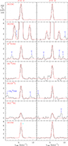 |
Fig. 1. J = 4 − 3 and J = 5 − 4 transitions of the single substituted isotopologs of HCCNC. The abscissa corresponds to the velocity with respect to the local standard of rest. The derived line parameters are given in Table A.1. The ordinate is the antenna temperature, corrected for atmospheric and telescope losses, in mK. Blanked channels correspond to negative features produced when folding the frequency-switched data. The red line shows the computed synthetic spectra for these lines (see Sect. 3.3). The second row panels correspond to a zoom in intensity of the lines of the main isotopolog (first row) to show the emission from its weak hyperfine components. The J = 4 − 3 line of DCCNC (marked with a cyan star) is affected by the negative features produced by the hyperfine structure of CH3CN which is ∼8 MHz above in frequency. |
Derived rotational constants and column densities for the isotopologs of HCCNC and HNCCC.
3.2. Spectroscopy of HNCCC
HNCCC was discovered in TMC-1 by Kawaguchi et al. (1992b) through the observation of three unknown lines in the Nobeyama spectral line survey of TMC-1 (Kaifu et al. 2004) that they assigned to this isomer of HCCCN. The dipole moment of this molecule has been computed through ab initio calculations to be 5.67 D (Botschwina et al. 1992). The molecule was observed in the laboratory by Hirahara et al. (1993) confirming the assignment of Kawaguchi et al. (1992b). These observations included the hyperfine components of the J = 1 − 0 and J = 2 − 1 transitions. Laboratory line frequencies up to J = 31 − 30 have been reported by Vastel et al. (2018). Several lines at 3 mm have been also observed with our data gathered with the IRAM 30 m radio telescope (see Fig. A.1). In addition, we have observed the hyperfine structure of the J = 4 − 3 and J = 5 − 4 lines with the QUIJOTE line survey (see Fig. 2). The derived line parameters for all observed transitions of HNCCC are given in Table A.1. All the spectroscopic data from the laboratory and our space observations were fitted with the same Hamiltonian than for HCCNC. The results are given in Table 1. Unlike the case of HCCNC, the only spectral information for the isotopologs of HNCCC concerns DNCCC (Hirahara et al. 1993). This isotopolog was observed in TMC-1 by Cernicharo et al. (2020). Improved frequencies for DNCCC are reported in Table A.1 and its derived rotational constants are given in Table 1. Assuming that the emission of HNCCC is not affected by line opacity, then we could expect to detect the lines from the 13C isotopologs at the level of 1–1.5 mK. For H15NCCC, the same lines should be at the level of 0.5 mK (assuming the HCCNC/HCC15NC abundance ratio). The expected molecular constants, B0 and D0, of the isotopologs have been computed through ab initio calculations using B0,exp(HNCCC)/Be, cal(HNCCC) as the scaling factor. We estimated B0 ∼ 4655.5, 4644.0, 4501.0, and 4545.4 MHz for HN13CCC, HNC13CC, HNCC13C, and H15NCCC, respectively. Three pairs of lines with similar intensities, as is the case for the isotopologs of HCCNC, have been easily found with a near perfect harmonic frequency relation 5/4 in our data close in frequency to our predictions. The deviation from this relation is 3 × 10⁻⁶ and fits the expected contribution of the distortion constant (∼0.6 kHz). They correspond to the three 13C isotopologs and they are shown in Fig. 2. Their line parameters are given in Table A.1. As only two lines are available for each isotopolog, we have adopted a distortion constant of 0.61 kHz for HN13CCC and HNC13CC, and of 0.57 kHz for HNCC13C. The derived rotational constants, for which we estimated a conservative uncertainty of 5 kHz, are given in Table 1. We have not been able to find a similar pair of lines that could be assigned to the 15N isotopolog because too many features do appear at the expected intensities of 0.5 mK. Thus, we report the first detection in space of the 13C isotopologs of HNCCC and the determination of their rotational constant.
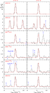 |
Fig. 2. Same as Fig. 1, but for HNCCC. The red line shows the computed synthetic spectra for these lines (see Sect. 3.3). The second row correspond to a zoom in intensity of the lines of the main isotopolog (first row). The derived line parameters are given in Table A.1. |
3.3. Rotational temperatures and column densities
We analyzed the intensities of the lines of HCCNC and HNCCC using a rotational diagram to derive the rotational temperatures of these molecules. We assumed a source of uniform brightness temperature and a radius of 40″ (Fossé et al. 2001, Fuentetaja et al., in prep.) to estimate the dilution factor for each transition. The line width adopted in the models to compute the synthetic spectra is 0.6 km s−1 for all lines. The results of the rotational diagram for HCCNC are Trot = 5.5 ± 0.1 K and N = (3.4 ± 0.1)×1012 cm−2, while for HNCCC, we obtained Trot = 4.5 ± 0.2 K and N = (5.8 ± 0.2)×1011 cm−2. The corresponding synthetic spectra are shown in Fig. 1 for HCCNC and in Fig. 2 for HNCCC. We note that the weak hyperfine satellite lines of HCCNC and HNCCC are very well reproduced with the derived values for the column densities. These hyperfine components represent 2% and 1.3% of the total intensity of the J = 4 − 3 and 5–4 transitions, respectively. The fact that the modeled intensities for the weak and strong hyperfine components are in perfect agreement with the observations indicates that the emission of the J = 4 − 3 and 5–4 transitions of HCCNC. In addition, HNCCC is mostly optically thin. Hence, the derived column densities can be used to obtain isotopic abundance ratios. By adopting the rotational temperatures derived for HCCNC and HNCCC for all their isotopologs, we obtained the column densities given in Table 1. The match between computed and observed spectra is excellent (see Figs. 1 and 2) and the derived isotopic abundance ratios are given in Table 2. We note that the synthetic spectra derived from the assumption of a constant rotational temperature reproduce the observed spectra at 3 mm for both species rather well. Nevertheless, the column density of HNCCC has to be reduced by a factor 1.5 to reproduce the observed intensities of this species at 3 mm.
Isotopic abundance ratios.
Collisional rates for HCCNC and HNCCC with p-H2 and o-H2 have been calculated by Bop et al. (2021). We used the large velocity gradient approximation (LVG), described by Goldreich & Kwan (1974) and implemented in the MADEX code (Cernicharo 2012), to model the line profiles of the J = 4 − 3 to J = 11 − 10 lines of both isomers. We explored the density and the column density that produce the best fit to the J = 8 − 7 to J = 11 − 10 lines of these species using p-H2 as collider. For HCCNC the best fit is obtained for n(H2) = (7.0 ± 0.3) × 103 cm−3 and N = (2.7 ± 0.2) × 1012 cm−2. The excitation temperatures vary between 7.3 K for the J = 4 − 3 transition to 4.7 K for the J = 11 − 10 one. The generated synthetic spectra are shown in blue in Fig. A.1. These synthetic spectra agree rather well with those obtained for a constant rotational temperature of 5.5 K and N = 3.4 × 1012 cm−2 (synthetic spectra shown in red in Fig. A.1). However, this fit to the volume density and column density to the 3 mm lines does not adequately reproduce the observations of the J = 4 − 3 and J = 5 − 4 lines. The differences between the two methods are probably related to the density structure of the source and to the accuracy of the collisional rates. We note that the derived density is lower than that derived from other molecules in TMC-1. We checked the effect of using o-H2 as collider and found similar results. In the case of HNCCC, our LVG calculations indicate that the intensity of the 3 mm lines are well reproduced, with n(H2) = 1.5 × 104 cm−3 and a column density of 3.8 × 10¹¹. The excitation temperatures vary between 5.6 K for the J = 4 − 3 transition to 4.0 K for the J = 11 − 10 one. The computed synthetic spectra are shown in blue in Fig. A.1 and agree well with those obtained from a constant rotational temperature (red curve in Fig. A.1). It is worth noting that in this case the derived volume density is in better agreement with the values derived from other species. We note also that as for HCCNC, the best column density obtained from the LVG analysis is lower than that obtained by the rotational diagram. The most plausible explanation for these differences in both isomers is related to the cloud density structure, that is, the dense core of TMC-1 can not be treated as an object of uniform density. Moreover, it is also likely that molecular abundances vary across the core.
4. Discussion
For the following discussion, we adopt the values derived above for the column densities using an uniform rotational temperature for all observed transitions. Taking the column density of HCCCN derived by Tercero et al. (2024) of 1.9 × 1014 cm−2, the relative abundance ratios are 56, 328, and 6 for HCCCN/HCCNC, HCCCN/HNCCC, and HCCNC/HNCCC, respectively. These values agree, within a factor of two, with those obtained from less sensitive line surveys of TMC-1 (Gratier et al. 2016). The derived abundance for the isotopologs of HCCNC, HNCCC, and HCCCN permits us to study the isotopic 12C/13C abundance ratio for the three possible substitutions. The results are given in Table 2. We found that for HCCNC and HNCCC this isotopic ratio does not depend on the substituted carbon, being very similar to the solar one and slightly larger than that of the local ISM of 59–76 (Lucas & Liszt 1998; Wilson 1999; Milam et al. 2005; Sheffer et al. 2007; Stahl et al. 2008; Ritchey et al. 2011). The results from Tercero et al. (2024) for HCCCN also indicate that for the most abundant isomer, the only isotopolog whose ratio is slightly different is HCC13CN. Table 2 presents a summary of these ratios.
The 13C isotopic ratios derived for HCCCN in TMC-1 are in agreement with previous determinations in other cold dense clouds, such as L1521B, L134N (Taniguchi et al. 2017), L1527 (Yoshida et al. 2019), and L483 (Agúndez et al. 2019); more specifically, HCC13CN is somewhat more abundant than the other two 13C isotopologs. The 12C/13C ratio for HCC13CN in TMC-1 is consistent with the local ISM 12C/13C ratio, while the isotopologs H13CCCN and HC13CCN are somewhat diluted in 13C. This behavior is reproduced by the chemical model of Loison et al. (2020), assuming that C3 reacts with oxygen atoms, although we caution that there are uncertainties in some of the relevant chemical reactions. In the cases of HCCNC and HNCCC, the three 13C isotopologs show similar abundances, somewhat above the local ISM 12C/13C ratio. A slight dilution in 13C was therefore found for the three isotopologs of HCCNC and HNCCC.
The dependence of the isotopic ratio between HC3N and carbon substituted HC3N on the position of the 13C was previously discussed by Taniguchi et al. (2016, 2017). They concluded that the main formation of HC3N comes from the neutral-neutral reaction between acetylene C2H2 and CN. The 13C substituted HC3N has been considered in the fractionation models of Loison et al. (2020), who obtained a satisfactory agreement with observations when introducing a moderate value for the C3 and O reaction rate coefficient. The most recent Letter by Sipilä et al. (2023) only introduces 13C fractionation reactions for CCH, C3, and c-C3H2. The three 13C isotopomers of HC3N thus have equal abundances over the full time dependence in the corresponding models.
The carbon and nitrogen isotopic chemistry of HCCNC and HNCCC has not seen very much interest until now and no chemical model has been performed to predict their isotopic ratios as yet. The deuterated species were detected by Cernicharo et al. (2020) and the abundance ratios were reported and modeled in Cabezas et al. (2021) with reasonable success. Interestingly, the recent detection of HCCNCH+ by Agúndez et al. (2022), showing a high HCCNCH+ over HCCNC ratio (on the order of 10−2), is surprisingly well reproduced in the associated chemical model. This is contrary to the results seen for most other protonated molecules. Following the KIDA database suggestion (Wakelam et al. 2012), we find that HCCNCH+ is efficiently formed through the C+ + CH3CN reaction that can return HCCNC through dissociative recombination amongst other products. This mechanism prevails over the other proton transfer reactions in our chemical model. Such an ion-molecule scheme may lead to different isotopic ratios than the neutral-neutral formation channels. Further studies on these topics are desirable to build on these results.
Q-band Ultrasensitive Inspection Journey to the Obscure TMC-1 Environment.
Acknowledgments
We thank Ministerio de Ciencia e Innovación of Spain (MICIU) for funding support through projects PID2019-106110GB-I00, PID2019-107115GB-C21/AEI/10.13039/501100011033, and PID2019-106235GB-I00. We also thank ERC for funding through grant ERC-2013-Syg-610256-NANOCOSMOS.
References
- Agúndez, M., Marcelino, N., Cernicharo, J., et al. 2019, A&A, 625, A147 [NASA ADS] [CrossRef] [EDP Sciences] [Google Scholar]
- Agúndez, M., Cabezas, C., Marcelino, N., et al. 2022, A&A, 659, L9 [NASA ADS] [CrossRef] [EDP Sciences] [Google Scholar]
- Bop, C. T., Lique, F., Faure, A., et al. 2021, MNRAS, 501, 1911 [Google Scholar]
- Botschwina, P., Horn, M., Seeger, S., & Flügge, J. 1992, Chem. Phys. Lett., 195, 427 [NASA ADS] [CrossRef] [Google Scholar]
- Cabezas, C., Roueff, E., Tercero, B., et al. 2021, A&A, 650, L15 [NASA ADS] [CrossRef] [EDP Sciences] [Google Scholar]
- Cabezas, C., Agúndez, M., Marcelino, N., et al. 2022, A&A, 657, L4 [NASA ADS] [CrossRef] [EDP Sciences] [Google Scholar]
- Cernicharo, J. 1985, Internal IRAM Report (Granada: IRAM) [Google Scholar]
- Cernicharo, J. 2012, in ECLA 2011: Proc. of the European Conference on Laboratory Astrophysics, eds. C. Stehl, C. Joblin, & L. d’Hendecourt (Cambridge: Cambridge Univ. Press), EAS Publ. Ser., 2012, 251, https://nanocosmos.iff.csic.es/?page_id=1619 [Google Scholar]
- Cernicharo, J., Marcelino, N., Rouef, E., et al. 2012, ApJ, 759, L43 [Google Scholar]
- Ceccarelli, C., Caselli, P., Bockelée-Morvan, D., et al. 2014, in Protostars and Planets VI, eds. H. Beuther, R. S. Kiessen, C. P. Dullemond, et al. (Univ. Arizona Press), 859 [Google Scholar]
- Cernicharo, J., Marcelino, N., Agúndez, M., et al. 2020, A&A, 642, L8 [NASA ADS] [CrossRef] [EDP Sciences] [Google Scholar]
- Cernicharo, J., Agúndez, M., Kaiser, R., et al. 2021, A&A, 652, L9 [NASA ADS] [CrossRef] [EDP Sciences] [Google Scholar]
- Cernicharo, J., Fuentetaja, R., Agúndez, M., et al. 2022, A&A, 663, L9 [NASA ADS] [CrossRef] [EDP Sciences] [Google Scholar]
- Cernicharo, J., Fuentetaja, R., Agúndez, M., et al. 2023, A&A, 680, L4 [NASA ADS] [CrossRef] [EDP Sciences] [Google Scholar]
- Colzi, L., Sipilä, O., Roueff, E., et al. 2020, A&A, 640, A51 [NASA ADS] [CrossRef] [EDP Sciences] [Google Scholar]
- Fossé, D., Cernicharo, J., Gerin, M., & Cox, P. 2001, ApJ, 552, 168 [Google Scholar]
- Goldreich, P., & Kwan, J. 1974, ApJ, 189, 441 [CrossRef] [Google Scholar]
- Gratier, P., Majumdar, L., Ohishi, M., et al. 2016, ApJS, 225, 25 [Google Scholar]
- Guarnieri, A., Hinze, R., Krüger, M., & Zerbe-Foese, H. 1992, J. Mol. Spectr., 156, 39 [NASA ADS] [CrossRef] [Google Scholar]
- Hirahara, Y., Ohshima, Y., & Endo, Y. 1993, ApJ, 403, L83 [CrossRef] [Google Scholar]
- Huckauf, A., Guarniere, A., Lentz, D., & Fayt, A. 1998, J. Mol. Spectr., 188, 109 [CrossRef] [Google Scholar]
- Kaifu, N., Ohishi, M., Kawaguchi, K., et al. 2004, PASJ, 56, 69 [Google Scholar]
- Kawaguchi, K., Ohishi, M., Ishikawa, S.-I., & Kaifu, N. 1992a, ApJ, 386, L51 [NASA ADS] [CrossRef] [Google Scholar]
- Kawaguchi, K., Takano, S., Ohishi, M., et al. 1992b, ApJ, 396, L49 [CrossRef] [Google Scholar]
- Krüger, M., Dreizler, H., Preugschat, D., & Lentz, D. 1991, Angew. Chem. Int. Ed. Engl., 30, 1644 [CrossRef] [Google Scholar]
- Krüger, M., Stahlm, W., & Dreizler, H. 1992, J. Mol. Spectr., 158, 298 [Google Scholar]
- Loison, J.-C., Wakelam, V., Gratier, P., & Hickson, K. M. 2020, MNRAS, 498, 4663 [Google Scholar]
- Lucas, R., & Liszt, H. 1998, A&A, 337, 246 [NASA ADS] [Google Scholar]
- Milam, S. N., Savage, C., Brewster, M. A., & Ziurys, L. M. 2005, ApJ, 634, 1126 [NASA ADS] [CrossRef] [Google Scholar]
- Müller, H. S. P., Schlöder, F., Stutzki, J., & Winnewisser, G. 2005, J. Mol. Spectr., 742, 215 [Google Scholar]
- Pardo, J. R., Cernicharo, J., & Serabyn, E. 2001, IEEE Trans. Antennas Propag., 49, 12 [Google Scholar]
- Pickett, H. M., Poynter, R. L., Cohen, E. A., et al. 1998, J. Quant. Spectrosc. Radiat. Transf., 60, 883 [Google Scholar]
- Ritchey, A. M., Federman, S. R., & Lambert, D. L. 2011, ApJ, 728, 36 [NASA ADS] [CrossRef] [Google Scholar]
- Roueff, E., Loison, J.-C., & Hickson, K. M. 2015, A&A, 576, A99 [NASA ADS] [CrossRef] [EDP Sciences] [Google Scholar]
- Sheffer, Y., Rogers, M., Federman, S. R., et al. 2007, ApJ, 667, 1002 [NASA ADS] [CrossRef] [Google Scholar]
- Sipilä, O., Colzi, L., Roueff, E., et al. 2023, A&A, 678, A120 [NASA ADS] [CrossRef] [EDP Sciences] [Google Scholar]
- Stahl, O., Casassus, S., & Wilson, T. 2008, A&A, 477, 865 [NASA ADS] [CrossRef] [EDP Sciences] [Google Scholar]
- Taniguchi, K., Saito, M., & Ozeki, H. 2016, ApJ, 830, 106 [NASA ADS] [CrossRef] [Google Scholar]
- Taniguchi, K., Ozeki, H., & Saito, M. 2017, ApJ, 846, 46 [NASA ADS] [CrossRef] [Google Scholar]
- Tercero, F., López-Pérez, J. A., Gallego, J. D., et al. 2021, A&A, 645, A37 [EDP Sciences] [Google Scholar]
- Tercero, B., Marcelino, N., Agúndez, M., et al. 2024, A&A, 682, L12 [NASA ADS] [CrossRef] [EDP Sciences] [Google Scholar]
- Vastel, C., Kawaguchi, K., Quénard, D., et al. 2018, MNRAS, 474, L76 [NASA ADS] [CrossRef] [Google Scholar]
- Wakelam, V., Herbst, E., Loison, J.-C., et al. 2012, ApJS, 199, 21 [Google Scholar]
- Wilson, T. L. 1999, Rep. Prog. Phys., 62, 143 [Google Scholar]
- Yan, Y. T., Henkel, C., Kobayashi, C., et al. 2023, A&A, 670, A98 [NASA ADS] [CrossRef] [EDP Sciences] [Google Scholar]
- Yoshida, K., Sakai, N., Nishimura, Y., et al. 2019, PASJ, 71, S18 [NASA ADS] [CrossRef] [Google Scholar]
Appendix A: Line parameters
Line parameters for all observed transitions were derived by fitting a Gaussian line profile to them using the GILDAS package. A velocity range of ±20 km s−1 around each feature was considered for the fit after a polynomial baseline was removed. Negative features produced in the folding of the frequency switching data were blanked before baseline removal. The derived line parameters for all observed lines are given in Table A.1. The J = 4-3 and J = 5-4 lines of HCCNC are shown in Fig. 1 and those of HNCCC in Fig. 2. The J = 8-7 to J = 11-10 lines of HCCNC and HNCCC are shown in Fig. A.1.
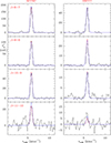 |
Fig. A.1. Observed lines in the 3mm domain of HCCNC (left panels) and HNCCC (right panels). The abscissa and ordinate are those of Fig. 1. The computed synthetic spectra adopting a constant rotational temperature are shown in red, whereas those obtained from the LVG model are shown in blue (see Sect. 3.3). The derived line parameters are given in Table A.1. |
Observed line parameters for the isotopologs of HCCNC and HNCCC
All Tables
Derived rotational constants and column densities for the isotopologs of HCCNC and HNCCC.
All Figures
|
Fig. 1. J = 4 − 3 and J = 5 − 4 transitions of the single substituted isotopologs of HCCNC. The abscissa corresponds to the velocity with respect to the local standard of rest. The derived line parameters are given in Table A.1. The ordinate is the antenna temperature, corrected for atmospheric and telescope losses, in mK. Blanked channels correspond to negative features produced when folding the frequency-switched data. The red line shows the computed synthetic spectra for these lines (see Sect. 3.3). The second row panels correspond to a zoom in intensity of the lines of the main isotopolog (first row) to show the emission from its weak hyperfine components. The J = 4 − 3 line of DCCNC (marked with a cyan star) is affected by the negative features produced by the hyperfine structure of CH3CN which is ∼8 MHz above in frequency. |
| In the text | |
|
Fig. 2. Same as Fig. 1, but for HNCCC. The red line shows the computed synthetic spectra for these lines (see Sect. 3.3). The second row correspond to a zoom in intensity of the lines of the main isotopolog (first row). The derived line parameters are given in Table A.1. |
| In the text | |
|
Fig. A.1. Observed lines in the 3mm domain of HCCNC (left panels) and HNCCC (right panels). The abscissa and ordinate are those of Fig. 1. The computed synthetic spectra adopting a constant rotational temperature are shown in red, whereas those obtained from the LVG model are shown in blue (see Sect. 3.3). The derived line parameters are given in Table A.1. |
| In the text | |
Current usage metrics show cumulative count of Article Views (full-text article views including HTML views, PDF and ePub downloads, according to the available data) and Abstracts Views on Vision4Press platform.
Data correspond to usage on the plateform after 2015. The current usage metrics is available 48-96 hours after online publication and is updated daily on week days.
Initial download of the metrics may take a while.