Constraining the H2 column densities in the diffuse interstellar medium using dust extinction and H I data

R. Skalidis; P. F. Goldsmith; P. F. Hopkins; S. B. Ponnada

doi:10.1051/0004-6361/202347968

Home

All issues

Volume 682 (February 2024)

A&A, 682 (2024) A161

Full HTML

Open Access

Issue		A&A Volume 682, February 2024


Article Number		A161
Number of page(s)		20
Section		Interstellar and circumstellar matter
DOI		https://doi.org/10.1051/0004-6361/202347968
Published online		21 February 2024

A&A, 682, A161 (2024)

Constraining the H₂ column densities in the diffuse interstellar medium using dust extinction and H I data^★

R. Skalidis¹^,2, P. F. Goldsmith², P. F. Hopkins³ and S. B. Ponnada³

¹ Owens Valley Radio Observatory, California Institute of Technology, MC 249-17, Pasadena, CA 91125, USA
e-mail: skalidis@caltech.edu
² Jet Propulsion Laboratory, California Institute of Technology, 4800 Oak Grove Drive, Pasadena, CA 91109-8099, USA
e-mail: paul.f.goldsmith@jpl.nasa.gov
³ California Institute of Technology, TAPIR, Mailcode 350-17, Pasadena, CA 91125, USA

Received: 14 September 2023
Accepted: 4 December 2023

Abstract

Context. Carbon monoxide (CO) is a poor tracer of H₂ in the diffuse interstellar medium (ISM), where most of the carbon is not incorporated into CO molecules, unlike the situation at higher extinctions.

Aims. We present a novel, indirect method for constraining H₂ column densities (N_H₂) without employing CO observations. We show that previously recognized nonlinearities in the relation between the extinction, A_V (H₂), derived from dust emission and the H I column density (N_H I) are due to the presence of molecular gas.

Methods. We employed archival (N_H₂) data, obtained from the UV spectra of stars, and calculated A_V(H₂) toward these sight lines using 3D extinction maps. The following relation fits the data: log N_H₂ = 1.38742 (log A_V(H₂)⁾³ − 0.05359 (log A_V(H₂)⁾² + 0.25722 log A_V(H₂) + 20.67191. This relation is useful for constraining N_H₂ in the diffuse ISM as it requires only N_H I and dust extinction data, which are both easily accessible. In 95% of the cases, the estimates produced by the fitted equation have deviations of less than a factor of 3.5. We constructed a N_H₂ map of our Galaxy and compared it to the CO integrated intensity (W_CO) distribution.

Results. We find that the average ratio (X_CO) between N_H₂ and W_CO is approximately equal to 2 × 10²⁰ cm⁻² (K km s⁻¹ )⁻¹, consistent with previous estimates. However, we find that the X_CO factor varies by orders of magnitude on arcminute scales between the outer and the central portions of molecular clouds. For regions with N_H₂ ≳ 10²⁰ cm⁻², we estimate that the average H₂ fractional abundance, f_H₂ = 2 N_H₂/(2N_H₂ + N_H I), is 0.25. Multiple (distinct) largely atomic clouds are likely found along high-extinction sightlines (A_V ≥ 1 mag), hence limiting f_H₂ in these directions.

Conclusions. More than 50% of the lines of sight with N_H₂ ≥ 10²⁰ cm⁻² are untraceable by CO with a J = 1−0 sensitivity limit W_CO = 1 K km s⁻¹.

Key words: methods: data analysis / ISM: abundances / dust, extinction / ISM: structure / Galaxy: abundances / local insterstellar matter

^★

A copy of the N_H₂ and X_CO maps is available at the CDS website/ftp to cdsarc.cds.unistra.fr (130.79.128.5) or via https://cdsarc.cds.unistra.fr/viz-bin/cat/J/A+A/682/A161

© The Authors 2024

Open Access article, published by EDP Sciences, under the terms of the Creative Commons Attribution License (https://creativecommons.org/licenses/by/4.0), which permits unrestricted use, distribution, and reproduction in any medium, provided the original work is properly cited.

This article is published in open access under the Subscribe to Open model. Subscribe to A&A to support open access publication.

1 Introduction

Molecular hydrogen is the most abundant molecule in the Universe, rendering it one of the most, if not the most, important chemical constituents. Molecular hydrogen’s lack of a permanent electric dipole moment results in its rotational levels being connected only by quadrupole transitions. Their weakness, together with the large spacing of its rotational levels, results in rotational emission from H₂ being extremely weak at the temperatures typically encountered in molecular regions and is only rarely observed in infrared emission.

An alternative method for observing molecular hydrogen is through absorption lines; molecular hydrogen has several Lyman–Werner absorption lines at UV wavelengths (11.2– 13.6 eV). The column density of H₂ can be determined by measuring the depths of the Lyman–Werner absorption lines against UV-bright background sources (Savage et al. 1977; Savage & Sembach 1996; Cartledge et al. 2004; Shull et al. 2021; Mangum & Shirley 2015).

The direct measurement of $N_{H_{2}}$ ${N_{{{\rm{H}}_2}}}$ , either through emission or absorption, requires space observatories. The Mid-Infrared Instrument (MIRl) spectrometer on board the James Webb Space Telescope (Rieke et al. 2015; Bouchet et al. 2015; Kendrew et al. 2015; Boccaletti et al. 2015; Wells et al. 2015; Glasse et al. 2015; Gordon et al. 2015; Wright et al. 2023) is sensitive to H₂ rotational transitions (e.g., Armus et al. 2023), while the absorption lines can be detected in spectra obtained with the Far Ultraviolet Spectroscopic Explorer or the Hubble Space Telescope (Savage et al. 1977; Bohlin et al. 1978; Shull et al. 2000, 2021; Sofia et al. 2005; Sheffer et al. 2008; Rachford et al. 2002, 2009; Gillmon et al. 2006). The necessity of space observatories makes $N_{H_{2}}$ ${N_{{{\rm{H}}_2}}}$ measurements expensive and thus relatively sparse. For this reason, various indirect techniques have been developed to estimate $N_{H_{2}}$ ${N_{{{\rm{H}}_2}}}$ . Below, we summarize the most widely applied indirect methods.

Dust emission is one of the most commonly applied indirect methods for constraining $N_{H_{2}}$ ${N_{{{\rm{H}}_2}}}$ . Emission from dust at far–infrared wavelengths (λ ≳ 100 µm) traces cold molecular gas; the dust in dark and giant molecular clouds emits thermal radiation as a gray–body. Using multiwavelength observations of dust emission, the dust spectral energy distribution can be obtained and fitted analytically with the following free parameters (e.g., Hildebrand 1983; Draine et al. 2007; Paradis et al. 2010, 2023; Kirk et al. 2010; Martin et al. 2012; Planck Collaboration XI 2014; Schnee et al. 2006; Juvela et al. 2018): (1) dust temperature and (2) dust grain emissivity, which, assuming a dust-to-gas mass ratio, can be converted to $N_{H_{2}}$ ${N_{{{\rm{H}}_2}}}$ . Dust spectral energy distribution fitting was the most common strategy applied to analyze Herschel images to obtain $N_{H_{2}}$ ${N_{{{\rm{H}}_2}}}$ toward several nearby interstellar clouds (e.g., André et al. 2010; Miville-Deschênes et al. 2010; Palmeirim et al. 2013; Könyves et al. 2010, 2015; Cox et al. 2016).

The use of carbon monoxide (CO) emission lines is another powerful method for probing $N_{H_{2}}$ ${N_{{{\rm{H}}_2}}}$ . CO is an abundant molecule in the ISM. It is abundant in regions where $N_{H_{2}} \geq 10^{20} {cm}^{- 2}$ ${N_{{{\rm{H}}_2}}} \ge {10^{20}}\,\,{\rm{c}}{{\rm{m}}^{ - 2}}$ , as self-shielding there is sufficient to prevent rapid photo-dissociation of CO by the background ISM radiation field. Thus, when there is CO, there is also H₂, although the opposite is not always true (e.g., Grenier et al. 2005; Planck Collaboration XIX 2011; Barriault et al. 2010; Langer et al. 2010, 2014, 2015; Velusamy et al. 2010; Pineda et al. 2013; Goldsmith 2013; Skalidis et al. 2022; Madden et al. 2020; Kalberla et al. 2020; Murray et al. 2018; Lebouteiller et al. 2019; Glover & Smith 2016; Seifried et al. 2020; Li et al. 2015).

The CO integrated intensity (W_CO) can be used as a proxy for $N_{H_{2}}$ ${N_{{{\rm{H}}_2}}}$ by employing the X_CO factor, defined as $N_{H_{2}} = X_{CO} W_{CO} .$ ${N_{{{\rm{H}}_2}}} = {X_{{\rm{CO}}}}{W_{{\rm{CO}}}}.$ (1)

In our Galaxy, the average value of X_CO is 〈X_CO〉 ≈ 2 × 10²⁰ cm⁻² (K km s⁻¹)⁻¹ (Bolatto et al. 2013). When X_CO is measured, factor of 2 deviations are expected from the average value due to the assumptions employed to estimate $N_{H_{2}}$ ${N_{{{\rm{H}}_2}}}$ by various methods (Dame et al. 2001; Bolatto et al. 2013).

The conversion of W_CO to $N_{H_{2}}$ ${N_{{{\rm{H}}_2}}}$ using the Galactic average X_CO is meaningful only in a statistical sense, and when it is applied on Galactic scales. Within individual clouds in the interstellar medium (ISM), X_CO can vary by orders of magnitude (e.g., Pineda et al. 2008, 2013; Lee et al. 2014; Ripple et al. 2013) due to the sensitivity of X_CO to local ISM conditions, including gas density, turbulent line width, and the interstellar radiation field (Visser et al. 2009; Glover & Clark 2016; Gong et al. 2017).

Diffuse regions of the ISM (defined as having A_V ≲ 1 mag, and density n ≲ 100 cm⁻³) may contain a significant fraction of molecular hydrogen but relatively little CO compared to the abundance of carbon (Grenier et al. 2005). The reason is that the formation of H₂ formation takes place at smaller extinctions than does that of CO due to the rapid onset of self-shielding at lower values of the extinction.

In the transition phase where the H₂ density has started rising but that of CO is still small, oxygen and carbon are largely in atomic form. In this region, then, H₂ is primarily associated with ionized (C⁺) or neutral (C I) carbon, and not with CO. Molecular hydrogen in regions that are undetectable in CO are referred to as CO-dark H₂. The mass of CO-dark H₂ is estimated to be ~30% of the total (primarily H₂) mass (Pineda et al. 2010; Kalberla et al. 2020).

Finally, $N_{H_{2}}$ ${N_{{{\rm{H}}_2}}}$ can be constrained using dust extinction. Dust in the ISM is well mixed with gas (Boulanger et al. 1996; Rachford et al. 2009). Thus, the extinction and reddening produced by dust is proportional to the total (atomic plus molecular hydrogen) gas column along the LOS (Bohlin et al. 1978). All established methodologies (Sect. 6) concur that in regions where the gas is atomic, the dust reddening, E(B − V), is linearly correlated with N_H I (Liszt & Gerin 2023; Lenz et al. 2017; Nguyen et al. 2018; Shull & Panopoulou 2023); changes in the dust or hydrogen content cause N_H I/E(B − V) to vary (Liszt 2014b; Shull & Panopoulou 2023). At high Galactic latitudes, Lenz et al. (2017) found that the linear correlation between E(B − V) and N_H I holds for N_H I ≲ 4 × 10²⁰ cm⁻². At higher H I column densities, E(B − V) increases nonlinearly with N_H I, behavior plausibly attributed to the presence of molecular gas. This implies that the residuals between the total dust extinction (or reddening) and the extinction induced by dust mixed with H I gas should probe $N_{H_{2}}$ ${N_{{{\rm{H}}_2}}}$ (Planck Collaboration XIX 2011; Paradis et al. 2012; Lenz et al. 2015; Kalberla et al. 2020).

This strategy for estimating $N_{H_{2}}$ ${N_{{{\rm{H}}_2}}}$ can only be applied if two conditions are satisfied: (1) the N_H I/E(B − V) ratio must be constrained, and (2) a mapping function that converts the extinction residuals to $N_{H_{2}}$ ${N_{{{\rm{H}}_2}}}$ exists. N_H I/E(B − V) has been constrained in the past by various authors (e.g., Liszt 2014b; Lenz et al. 2017; Nguyen et al. 2018; Shull et al. 2021). The major challenge is to find an accurate way to convert the extinction residuals to $N_{H_{2}}$ ${N_{{{\rm{H}}_2}}}$ .

In this paper, we present a novel method for converting the dust extinction residuals to $N_{H_{2}}$ ${N_{{{\rm{H}}_2}}}$ and then construct a full-sky $N_{H_{2}}$ ${N_{{{\rm{H}}_2}}}$ map of our Galaxy without using CO observations. We use our $N_{H_{2}}$ ${N_{{{\rm{H}}_2}}}$ estimates to constrain some of the molecular gas properties of our Galaxy.

We calculated the residuals between the total extinction and the extinction expected from dust mixed with H I gas toward lines of sight (LOSs) with $N_{H_{2}}$ ${N_{{{\rm{H}}_2}}}$ measurements; these $N_{H_{2}}$ ${N_{{{\rm{H}}_2}}}$ measurements have been obtained from absorption lines (Sect. 2). We find that the extinction residuals are well correlated with $N_{H_{2}}$ ${N_{{{\rm{H}}_2}}}$ and fit them with a polynomial function. We then calculated the extinction residuals using full-sky N_H I and E(B − V) maps (Sect. 3). Finally, we converted the extinction residuals to $N_{H_{2}}$ ${N_{{{\rm{H}}_2}}}$ using our fitted function in order to construct a full-sky $N_{H_{2}}$ ${N_{{{\rm{H}}_2}}}$ map at 16′ resolution.

We compared our constructed $N_{H_{2}}$ ${N_{{{\rm{H}}_2}}}$ map with the CO intensity map of Dame et al. (2001) (Sect. 4), reproducing the previously reported global value of X_CO. Our $N_{H_{2}}$ ${N_{{{\rm{H}}_2}}}$ estimates are consistent with previous work that combines dust extinction residuals and the X_CO factor (Sect. 4.2). We constructed a full-sky map of the molecular fractional abundance and show that molecular hydrogen is less abundant than atomic hydrogen (Sect. 5). In Sect. 5.2, we determine the proportion of CO-dark molecular hydrogen in relation to the total amount of molecular hydrogen. We explored the N_H/A_V ratio and compared our findings against previous results (Sect. 6). In Sects. 7 and 8, we discuss our results in the context of the existing literature and present our conclusions.

2 Probing molecular gas using dust extinction

For atomic gas, Lenz et al. (2017) found that dust reddening correlates with the column density of the atomic hydrogen as N_H I/E(B − V) = 8.8 × 10²¹ cm⁻² mag⁻¹. This is our reference value, and we show that our results remain statistically the same when we consider variations about this ratio (Sect. 2.2.2). When the gas becomes molecular, E(B − V) increases nonlinearly with respect to N_H I.

We assumed a constant total-to-selective extinction R_V = A_V/E(B − V) = 3.1 (Cardelli et al. 1989; Schlafly & Finkbeiner 2011) and calculated the visual extinction of dust mixed with atomic gas, $A_{V} (H I) = 0.35 \times 10^{- 21} N_{H I} .$ ${A_{\rm{V}}}({\rm{HI}}) = 0.35 \times {10^{ - 21}}{N_{{\rm{HI}}}}.$ (2)

R_V fluctuates throughout our Galaxy (e.g., Peek & Schiminovich 2013; Zhang et al. 2023). However, the uniformity of R_V is implicit in our method, because we employed dust reddening maps that were constructed using far-infrared multiwavelength dust intensity data (Sect. 3, Appendix A). These maps directly constrain the dust emission properties, such as dust temperature and opacity, when some dust model is fitted to the data, and indirectly E(B − V), by assuming some extinction law and R_V = 3.1 (e.g., Schlegel et al. 1998). In addition, most of the existing constraints of N_H I/E(B − V) also rely on these dust reddening maps. Therefore, the uniformity of R_V inevitably propagates in our methods and accounts for some of our uncertainties, which are calculated in Sect. 2.4.

We defined the residuals between the total dust extinction and A_V(H I) as $A_{V} (H_{2}) = A_{V} (H) - A_{V} (H I),$ ${A_{\rm{V}}}\left( {{{\rm{H}}_2}} \right) = {A_{\rm{V}}}({\rm{H}}) - {A_{\rm{V}}}({\rm{HI}}),$ (3)

where A_V(H) denotes the total extinction from dust associated with both atomic and molecular hydrogen. On the left hand side, we use H₂ in the parentheses because we hypothesize, and verify below (Fig. 1), that these residuals trace the visual extinction of dust mixed with molecular hydrogen.

Equation (3) is the cornerstone of our methodology for estimating $N_{H_{2}}$ ${N_{{{\rm{H}}_2}}}$ . A_V(H I) can be estimated using N_H I measurements (Eq. (2)) from surveys such as HI4PI (HI4PI Collaboration 2016), while A_V(H) can be extracted from publicly available full-sky dust extinction maps (e.g., Schlegel et al. 1998; Planck Collaboration Int. XXXV 2016). The next step in our strategy is to find an empirical relation for $N_{H_{2}}$ ${N_{{{\rm{H}}_2}}}$ as a function of A_V(H₂). Before proceeding, we discuss some pathologies in the definition of A_V(H₂).

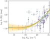Fig. 1

Extinction of dust mixed with molecular gas as a function of $N_{H_{2}}$ ${N_{{{\rm{H}}_2}}}$ . The H₂ column densities were determined from UV observations toward stars, and the A_V(H₂) were determined from the nonlinearities of the E(B − V) versus N_H I relation (Eq. (3)). Green stars identify outlying points that were not considered in the fitting. At high column densities, A_V(H₂) is strongly correlated with $N_{H_{2}}$ ${N_{{{\rm{H}}_2}}}$ , indicating that the nonlinear increase in dust reddening with respect to N_H I is induced by the presence of molecular gas. The orange curves were randomly sampled from the posterior distribution of the Markov chain Monte Carlo fitting, representing the fitting uncertainties. The green curve corresponds to the mean posterior profile that we employ to convert A_V(H₂) to $N_{H_{2}}$ ${N_{{{\rm{H}}_2}}}$ (Eq. (6)).

2.1 Pathologies in the definition of A_V (H₂)

Dust extinction is a positive definite quantity, but A_V(H₂) can become negative if A_V(H I) > A_V(H). This situation can be encountered when either the signal-to-noise ratio (S/N) of the measurements is low or the value of N_H I/E(B − V) deviates from its global value; variations of this ratio propagate to A_V(H₂), due to Eq. (3) (Sect. 2.2.2). We present a thought experiment to demonstrate how the use of a global N_H I/E(B − V) (Eq. (2)) can affect the estimation of A_V(H₂).

Consider an ISM cloud with a local N_H I/E(B − V) ratio smaller than the Galactic value. We considered the imaginary cloud to have a given A_V(H) and that the gas is atomic. Thus, the total extinction of the cloud will be produced by dust mixed with H I gas. If we used the local N_H I/E(B − V) of the cloud, we would derive that A_V(H) = A_V(H I), and hence A_V(H₂) = 0. However, in Eq. (3) we use the global value from Lenz et al. (2017), which would yield for the cloud of our thought experiment that A_V(H) < A_V(H I), and hence A_V(H₂) < 0.

Thus, A_V(H₂) can become negative due to the use of a global N_H I/E(B − V), which limits the detectability of our method. However, this is something that we cannot overcome because local measurements are limited. For this reason, for every measurement with A_V(H₂) < 0, we considered gas to be fully atomic, and it is not considered in the analysis below.

2.2 Mapping A_V (H₂) to $N_{H_{2}}$ ${N_{{{\rm{H}}_2}}}$

We calculated A_V(H₂) using Eq. (3) toward several LOSs with reliable direct $N_{H_{2}}$ ${N_{{{\rm{H}}_2}}}$ determinations. The direct $N_{H_{2}}$ ${N_{{{\rm{H}}_2}}}$ measurements were obtained by observing the Lyman–Werner absorption lines toward background sources in our Galaxy. We extracted the $N_{H_{2}}$ ${N_{{{\rm{H}}_2}}}$ measurements, with their corresponding observational uncertainties, from the catalogues of Sheffer et al. (2008), Gillmon et al. (2006), Gudennavar et al. (2012), and Shull et al. (2021); these catalogues also provide estimates for N_H I, which allow us to obtain A_V(H I) (Eq. (2)). For measurements with asymmetric observational uncertainties, we calculated their average value.

The majority of the sources used for estimating $N_{H_{2}}$ ${N_{{{\rm{H}}_2}}}$ are nearby – at distances of less than 1 kpc – and close to the Galactic plane. Therefore, the column densities obtained from the absorption lines of these stars trace the integrated gas abundances up to the distance of each object, and not the total gas column. Therefore, we also needed to calculate the dust extinction up to the distance of each star (d_★). Below, we explain how we obtained fractional extinctions up to the distance of each star using the publicly available 3D extinction map of Green et al. (2019).

For each object with $N_{H_{2}}$ ${N_{{{\rm{H}}_2}}}$ measurement, we extracted d_★ from the catalogue of Bailer-Jones et al. (2021), which uses parallaxes from Gaia Data Release 3 (Gaia Collaboration 2021). We then calculated the dust extinction integral of each star as $E {(B - V)}_{⋆} = \int_{0}^{d_{⋆}} d z E (B - V) (z),$ $E{(B - V)_ \star } = \mathop \smallint \nolimits^ _0^{{d_ \star }}{\rm{d}}zE(B - V)(z),$ (4)

where z is the LOS distance between the observer and the star at distance d_★, and E(B − V)(z) denotes the dust reddening at a given distance z. We extracted the E(B − V)(z) values from the 3D map (Bayestar19) of Green et al. (2019)¹. This map provides a sample of E(B − V)(z) profiles drawn from a posterior distribution; for the calculation of E(B − V)_★ we used the most probable extinction profile. Dust reddening values from the map of Green et al. (2019) are calibrated for the Sloan Digital Sky Survey (SDSS) bands. We converted to dust reddening by multiplying the output of their map by 0.884, which is the standard color correction recommended by those authors. Then, we converted E(B − V)_★ to A_V(H) by multiplying by R_V.

Both A_V(H) and A_V(H I) are constrained for the LOSs where $N_{H_{2}}$ ${N_{{{\rm{H}}_2}}}$ measurements exist from spectroscopic observations. This allows us to calculate A_V(H₂) for each LOS and compare with $N_{H_{2}}$ ${N_{{{\rm{H}}_2}}}$ . Several objects with spectroscopically constrained $N_{H_{2}}$ ${N_{{{\rm{H}}_2}}}$ are located in the anticenter of our Galaxy, which are not covered by the extinction map of Green et al. (2019). These measurements were not considered in the analysis below.

Figure 1 displays A_V(H₂) versus $N_{H_{2}}$ ${N_{{{\rm{H}}_2}}}$ . We do not show measurements with log A_V(H₂) (mag) ≲ −1.2 because they are non-detections. We also note that some measurements, mostly with low S/N, yielded negative A_V(H₂). These were also discarded.

For log $N_{H_{2}} ({cm}^{- 2}) ≲ 19$ ${N_{{{\rm{H}}_2}}}\,\,\left( {{\rm{c}}{{\rm{m}}^{ - 2}}} \right) \mathbin{\lower.3ex\hbox{$\buildrel<\over {\smash{\scriptstyle\sim}\vphantom{_x}}$}} 19$ , A_V(H₂) remains constant with respect to $N_{H_{2}}$ ${N_{{{\rm{H}}_2}}}$ . Most of the measurements there have S/N < 3², and hence we cannot confidently determine whether the flatness of the profile is physical or induced by noise in the data. We observe a strong correlation between A_V(H₂) and $N_{H_{2}}$ ${N_{{{\rm{H}}_2}}}$ for log $N_{H_{2}} \geq 20$ ${N_{{{\rm{H}}_2}}} \ge 20$ . This correlation strongly supports the initial hypothesis that the extinction residuals, found in the total dust extinction when the extinction induced by dust mixed with H I is subtracted, yield the extinction of dust mixed with H₂ (as given by Eq. (3)).

The various quantities involved in our analysis (E(B − V), $N_{H_{2}}$ ${N_{{{\rm{H}}_2}}}$ , N_H I) are measured with beams of differing size: a) $N_{H_{2}}$ ${N_{{{\rm{H}}_2}}}$ is measured from UV absorption lines with a “pencil beam” defined by the star, b) several N_H I measurements have been constrained by fitting the Lyα profiles (e.g., as in Shull et al. 2021), which are also characterized by pencil beams, while some of the N_H I measurements were obtained from H I emission line data, where the resolution is 16′ (HI4PI Collaboration 2016), and c) the resolution of the 3D extinction map of Green et al. (2019) varies from 3.4′ to 13.7′. Some of the scatter of the points in Fig. is a result of this effect, but we note that the beam mismatch seems to be less important for diffuse and extended ISM clouds (e.g., Pineda et al. 2017; Murray et al. 2018). Although we cannot make a correction for this issue, we include it when we calculate the confidence levels of our method (Sect. 2.4).

2.2.1 Observational uncertainties in A_V (H₂)

There are two different sources of uncertainty that affect the estimates of A_V(H₂): (1) Uncertainties coming from the 3D extinction map of Green et al. (2019), and (2) distance uncertainties of stars.

To evaluate the dust extinction uncertainties, we sampled 300 random values from the posterior distribution of the Green et al. (2019) map at the most probable distance of each star (d_★). We calculated the extinction spread (σ_ext) at d_★.

Parallax uncertainties affect the distance estimates of a star. We consider the distance upper and lower limits denoted as d_★,+ and d_★,−, respectively. From the map of Green et al. (2019), we calculated the most probable extinction at d_★,+, and at d_★,−, denoted as E(B − V) and E(B − V) (d_★,−), respectively. We then calculated the differences σ_d+ = E(B − V) − E(B − V) (d_★) and σ_d− = E(B − V) d_★ − E(B − V) (d_★,−). The average (σ_d) between σ_d+ and σ_d− measures the extinction uncertainties due to parallax uncertainties. We take the total dust extinction uncertainty to be the quadratic sum of σ_ext and σ_d. These uncertainties are shown as the error bars in Fig. 1 and discussed in the following.

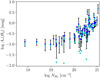Fig. 2

Same as Fig. 1 but for different N_H I/E(B − V) ratios. The black points with error bars correspond to our formal measurements using the N_H I/E(B − V) constraint of Lenz et al. (2017). Blue and cyan points correspond to measurements obtained when we assume that N_HI/E(B − V) × 10⁻²¹ is equal to 10 and 8 cm² mag⁻¹, respectively. Approximately all data points show statistically consistent results.

2.2.2 Uncertainties from N_H I/E(B − V) variations

At high Galactic latitudes (|b| ≥ 60°), Lenz et al. (2017) found that the correlation between E(B − V) and N_H I is very tight, with intrinsic variations only 0.015 mag. However, as shown recently by Shull & Panopoulou (2023), the uncertainties in the E(B − V) versus N_H I relation are larger than what is inferred by Lenz et al. (2017), with variations being dominated by systematic uncertainties in the employed datasets.

Lenz et al. (2017) used the E(B − V) map of Schlegel et al. (1998), and N_H I estimated using only emission line data from HI4PI Collaboration (2016), assuming that the line is optically thin. However, the E(B − V) values of Planck Collaboration XI (2014) are systematically larger than the values of Schlegel et al. (1998) at high Galactic latitudes (Shull & Panopoulou 2023). Thus, if the Planck map were employed, the ratio between N_H I and E(B − V) would be biased toward smaller values than what would have been inferred from the Schlegel et al. (1998) map. In addition, beam effects in the H I emission data can induce significant scatter in the obtained N_H I constraints. Several of these uncertainties are summarized in Shull & Panopoulou (2023), who found that N_H I/E(B − V) ×10⁻²¹ ranges from 8 to 10 cm⁻² mag⁻¹; this range is orders of magnitude larger than what is claimed by Lenz et al. (2017), and represents the formal uncertainty in N_H I/E(B − V). We explored how N_H I/E(B − V) variations, which propagate to our calculations through Eq. (2), affect our results.

Figure 2 shows A_V(H₂) versus $N_{H_{2}}$ ${N_{{{\rm{H}}_2}}}$ for every measurement, except for the outliers (green stars), shown in Fig. 1. Black points correspond to A_V(H₂) when we use the Lenz et al. (2017) relation, N_H I/E(B − V) ×10⁻²¹ = 8.8 cm⁻² mag⁻¹; the error bars are calculated as explained in Sect. 2.2.1. The blue and cyan points correspond to the obtained A_V(H₂) when we assume that N_HI/E(B − V) ×10⁻²¹ is equal to 10 and 8 cm⁻² mag⁻¹, respectively.

For log $N_{H_{2}} > 20.56$ ${N_{{{\rm{H}}_2}}} > 20.56$ , the colored (black and cyan) points are very close to the black points. In this regime, gas is mostly molecular, and thus the contribution of the dust mixed with atomic gas to the total dust extinction is minor. Thus, the uncertainty of N_H I/E(− V) has a weak effect in high-extinction regions. When $N_{H_{2}}$ ${N_{{{\rm{H}}_2}}}$ is low, deviations between black and colored points become more prominent, because the relative abundance of atomic gas is higher there. However, even there, the offset between the black and the colored points is statistically insignificant for the vast majority of the points (Fig. 2). There are only six exceptions, but this is only a minor fraction of the sample.

We conclude that our analysis remains robust in relation to variations of N_H I/E(B − V), which implies that uncertainties coming from the 3D extinction maps (Green et al. 2019) or Gaia distances (Sect. 2.2.1) are more important. However, variations in N_H I/E(B − V) likely contribute to the scatter of the observed $A_{V} (H_{2}) - N_{H_{2}}$ ${A_{\rm{V}}}\left( {{{\rm{H}}_2}} \right) - {N_{{{\rm{H}}_2}}}$ relation (Fig. 1). Our estimated confidence intervals include all the aforementioned uncertainties (Sect. 2.4).

2.3 Fitting the data

We fitted a polynomial to the $A_{V} (H_{2}) - N_{H_{2}}$ ${A_{\rm{V}}}\left( {{{\rm{H}}_2}} \right) - {N_{{{\rm{H}}_2}}}$ relation using Bayesian analysis. We assumed uniform priors, and calculated the following likelihood: $\ln ℒ = - {\sum }_{i = 1}^{N} [\ln \sqrt{2 π} + \ln σ + \frac{{(y_{i} - \tilde{y})}^{2}}{2 σ^{2}}],$ $\ln {\cal L} = - \mathop {\mathop \sum \nolimits^ }\limits_N^{i = 1} \left[ {\ln \sqrt {2\pi } + \ln \sigma + {{{{\left( {{y_i} - \tilde y} \right)}^2}} \over {2{\sigma ^2}}}} \right],$ (5)

where σ is the quadratic sum of the observational uncertainties of log A_V(H₂), and log $N_{H_{2}}$ ${N_{{{\rm{H}}_2}}}$ , y_i corresponds to the measured A_V(H₂), $\tilde{y}$ $\widetilde y$ is the intrinsic model, which we assume to be a polynomial, and i is the measurement index.

We sampled the parameter space with the “emcee” Markov chain Monte Carlo sampler (Foreman-Mackey et al. 2013). Measurements shown as green stars in Fig. 1 were not included in the fit because they are variable sources (Sect. 2.2.1). However, the fit changes only slightly even if they are included.

The best-fit polynomial equation is $\begin{matrix} \log A_{V} (H_{2}) = 0.03077 {(\log N_{H_{2}})}^{3} - 1.60469 {(\log N_{H_{2}})}^{2} \\ + 27.80868 \log N_{H_{2}} - 161.06073, \end{matrix}$ $\matrix{ {\log {A_{\rm{V}}}\left( {{{\rm{H}}_2}} \right) = 0.03077{{\left( {\log {N_{{{\rm{H}}_2}}}} \right)}^3} - 1.60469{{\left( {\log {N_{{{\rm{H}}_2}}}} \right)}^2}} \cr { + 27.80868\log {N_{{{\rm{H}}_2}}} - 161.06073,} \cr }$ (6)

with uncertainties for the fitted coefficients (from highest to smallest power of the logarithm) being 0.00769, 0.42823, 7.88171, and 49.91439. The spread of the fit, shown by the orange lines in Fig. 1, grows for log $N_{H_{2}} ({cm}^{- 2}) < 19$ ${N_{{{\rm{H}}_2}}}\,\,\left( {{\rm{c}}{{\rm{m}}^{ - 2}}} \right) < 19$ , making our fit unreliable in that range. This determines the sensitivity threshold of our method.

In practice, $N_{H_{2}}$ ${N_{{{\rm{H}}_2}}}$ is usually the unknown, while A_V(H₂) can be measured from dust extinction and N_H I observational data. $N_{H_{2}}$ ${N_{{{\rm{H}}_2}}}$ can be estimated from A_V(H₂) using the following analytical relation, which also fits our data well, $\begin{matrix} \log N_{H_{2}} = 1.38742 {(\log A_{V} (H_{2}))}^{3} - 0.05359 {(\log A_{V} (H_{2}))}^{2} \\ + 0.25722 \log A_{V} (H_{2}) + 20.67191. \end{matrix}$ $\matrix{ {\log {N_{{{\rm{H}}_2}}} = 1.38742{{\left( {\log {A_{\rm{V}}}\left( {{{\rm{H}}_2}} \right)} \right)}^3} - 0.05359{{\left( {\log {A_{\rm{V}}}\left( {{{\rm{H}}_2}} \right)} \right)}^2}} \cr { + 0.25722\log {A_{\rm{V}}}\left( {{{\rm{H}}_2}} \right) + 20.67191.} \cr }$ (7)

The fitting uncertainties of the coefficients, from highest to smallest power of the logarithm, are 0.17822, 0.17277, 0.05248, and 0.01555. The above equation maps A_V(H₂) to $N_{H_{2}}$ ${N_{{{\rm{H}}_2}}}$ , and we used it to construct a full-sky $N_{H_{2}}$ ${N_{{{\rm{H}}_2}}}$ map of our Galaxy (Sect. 3).

2.3.1 Fitting different polynomials

We experimented with the degree of the polynomial used to fit Eq. (7). For even polynomials, we find that $N_{H_{2}}$ ${N_{{{\rm{H}}_2}}}$ is reduced at high A_V(H₂) because the coefficient of the highest power of the fitted polynomial is always negative, hence making the curve concave downward. When we forced the coefficient of the highest-power term to be positive (by employing this constraint in the prior distribution), the reduction of $N_{H_{2}}$ ${N_{{{\rm{H}}_2}}}$ disappeared. However, we wish to keep a flat distribution of priors over the entire domain range (uninformative priors). We thus decided to work with polynomials whose highest-power term is odd because they did not show any reduction of $N_{H_{2}}$ ${N_{{{\rm{H}}_2}}}$ at high A_V(H₂).

A linear polynomial would not reproduce the nonlinear behavior of the data at log $N_{H_{2}} ({cm}^{- 2}) ≲ 20$ ${N_{{{\rm{H}}_2}}}\left( {{\rm{c}}{{\rm{m}}^{ - 2}}} \right) \mathbin{\lower.3ex\hbox{$\buildrel<\over {\smash{\scriptstyle\sim}\vphantom{_x}}$}} 20$ , and log A_V(H₂) (mag) ≲ −1 (Fig. 1). As a result, linear models would underestimate $N_{H_{2}}$ ${N_{{{\rm{H}}_2}}}$ in low-extinction regions. We conclude that a cubic polynomial (as shown in Eq. (7)) is the simplest function that accurately represents the data, while higher-degree polynomials overfit the data.

2.3.2 Outliers in the $A_{V} (H_{2}) - N_{H_{2}}$ ${A_{\rm{V}}}\left( {{H_2}} \right) - {N_{{{\rm{H}}_2}}}$ relation

In the fitting process, we excluded the four measurements shown as green stars (Fig. 1). According to the SIMBAD database, one of the outliers (identified as HD 200120) is a Be star – this object also appears in the Be star catalogue of the International Astronomical Union (Jaschek & Egret 1982), hence further supporting the validity of the spectral classification of this object – while there is a T Tauri (HD 40111) and a β Cephei variable (HD 172140) star. Both Be and T Tauri stars can show some variability in both photometric and spectroscopic observations: Be stars eject material, due to their rapid rotation, while the brightness of T Tauri objects can vary significantly, due to their high accretion rate, even within months. β Cephei are B-type stars whose surface pulsates owing to their rapid rotation. The last object that was considered an outlier (HD 164816) is a Be star according to the SIMBAD database. However, accurate spectroscopic observations suggest that it is a binary system (Sota et al. 2014). In either case, some degree of variability is expected, which explains why this measurement is an outlier. We consider the $N_{H_{2}}$ ${N_{{{\rm{H}}_2}}}$ measurements toward these stars to be untrustworthy and did not include them in the fit. But even if we include these measurements, the fit changes insignificantly.

2.4 Confidence intervals in the estimated $N_{H_{2}}$ ${N_{{H_2}}}$

Our fitted model (Eq. (7)) allows us to estimate $N_{H_{2}}$ ${N_{{{\rm{H}}_2}}}$ using H I and E(B − V) data. But the estimates do not come without uncertainties.

The uncertainties of the fit (shown by the orange lines in Fig. 1) are much smaller than the variance of the points about the fitted curve. These measured variations could be induced by several factors, such as variations in N_H I/E(B − V) (Sect. 2.2.2), R_V variations, metallicity gradients, H I emission line optical depth effects (Sect. 7), or due to the beam mismatch of the employed data, unaccounted for in our model. Therefore, the fitting uncertainties alone overestimate our confidence on the $N_{H_{2}}$ ${N_{{{\rm{H}}_2}}}$ estimates derived by Eq. (7).

To place reasonable confidence levels, we assumed that the depicted A_V(H₂) spread (Fig. 1) represents the intrinsic spread in our Galaxy. We calculated the linear scale ratio (r) between the observed A_V(H₂) with the value obtained from Eq. (7) for every data point with S/N ≥ 3. From the cumulative distribution function of r – the distribution of r is asymmetric with skewness equal to 1.38 – we obtained the following probabilities: for 68% of the measurements r ϵ [0.75, 2.48], for 95% r ϵ [0.46, 3.54], and for 99% r ϵ [0.30, 4.78]. This implies that in 95% of the cases, the “true” $N_{H_{2}}$ ${N_{{{\rm{H}}_2}}}$ should not deviate by a factor greater than 3.5 from the values obtained from the fit (Eq. (7)).

3 Full-sky N_H₂ map of our Galaxy

We use the N_H I data from the HI4PI survey (HI4PI Collaboration 2016) and the dust extinction map of Schlegel et al. (1998) – the values of this map are multiplied by 0.884 to account for systematic uncertainties (Schlafly et al. 2010; Schlafly & Finkbeiner 2011) – to construct a full-sky $N_{H_{2}}$ ${N_{{{\rm{H}}_2}}}$ map of our Galaxy. For comparison, we use the Planck extinction map. Overall, the Planck map shows enhanced extinction at high Galactic latitudes; this is also noted by Shull & Panopoulou (2023). The various estimated quantities for the molecular hydrogen do not change by more than a factor of 2 when the Planck map is used (Appendix A).

For the construction of the full-sky $N_{H_{2}}$ ${N_{{{\rm{H}}_2}}}$ map, we calculated A_V(H₂) using the N_H I and the E(B − V) maps (Eq. (3)), and then converted to $N_{H_{2}}$ ${N_{{{\rm{H}}_2}}}$ (Eq. (7)). The resolution of the extinction map (6.1′) is higher than that of the N_H I data (16.2′). We thus smoothed the extinction map to the resolution of the H I data. Figure 3 (top panel) shows a Mollweide projection of our constructed $N_{H_{2}}$ ${N_{{{\rm{H}}_2}}}$ map for the Milky Way. We only visualize regions with log $N_{H_{2}} \geq 19$ ${N_{{{\rm{H}}_2}}} \ge 19$ because below this limit our calibration relation is dominated by noise (Fig. 1).

We identify several molecular clouds of the Gould Belt, including the Polaris Flare (ℓ, b ~ 125°, +30°), Taurus (ℓ, b ~ 170°, −15°), and Orion (ℓ, b ~ 209°, −19°). The North Polar Spur appears as a large-scale molecular feature centered at Galactic coordinates ℓ, b ~ 15°, 15° and extending up to b ~ 45°. We observe many small-angular-scale diffuse molecular clouds in the southern Galactic hemisphere, while in the northern hemisphere molecular structures seem to be coherent over scales of many degrees.

We hardly see any molecular gas structures with log $N_{H_{2}} ({cm}^{- 2}) \geq 19$ ${N_{{{\rm{H}}_2}}}\,\,\left( {{\rm{c}}{{\rm{m}}^{ - 2}}} \right) \ge 19$ above the Galactic plane, for |b| ≥ 60°. This, however, seems to be the case only when we use the Schlegel et al. (1998) extinction map. When we construct the $N_{H_{2}}$ ${N_{{{\rm{H}}_2}}}$ map using extinctions from Planck Collaboration XII (2020), we see some molecular structures extending up to the northern and southern poles, and weaker emission from both extended and small-scale clouds at higher Galactic latitudes (Fig. A.1). In both $N_{H_{2}}$ ${N_{{{\rm{H}}_2}}}$ maps (Figs. 3, and A.1), the majority of the molecular gas seems to lie within |b| ≲ 45°.

In the Galactic plane, extinctions are larger than the extinction range used for the fitting of the $N_{H_{2}} - A_{V} (H_{2})$ ${N_{{{\rm{H}}_2}}} - {A_{\rm{V}}}\left( {{{\rm{H}}_2}} \right)$ relation (Eq. (7)). Therefore, the estimated H₂ column densities in the Galactic plane were derived by extrapolating the fitted relation to larger values of A_V.

4 Comparison with previous results

4.1 Comparing N_H₂ and W_CO

Figure 3 shows our $N_{H_{2}}$ ${N_{{{\rm{H}}_2}}}$ map (top panel) and the CO (J = 1−0) integrated intensity, W_CO, map (bottom panel) from Dame et al. (2001). The two maps are well correlated, but the observed structures in the $N_{H_{2}}$ ${N_{{{\rm{H}}_2}}}$ map are more extended than in W_CO. In this section our analysis is focused on CO-bright H₂ regions, while in Sect. 5.2 we study the properties of CO-dark H₂, which extends to higher Galactic latitudes than CO-bright H₂.

Figure 4 shows the full-sky X_CO (Eq. (1)) map obtained with our $N_{H_{2}}$ ${N_{{{\rm{H}}_2}}}$ measurements and W_CO from Dame et al. (2001). We calculated X_CO toward LOSs with W_CO ≥ 1 K km s⁻¹, which is the noise level in the CO data. We find that the average value of X_CO is approximately equal to 2 × 10²⁰ cm⁻² (K km s⁻¹)⁻¹, which matches exactly with the previously reported value (Bolatto et al. 2013; Liszt & Gerin 2016).

We observe that in many regions X_CO varies by orders of magnitude within a few arcminutes. The small-scale variations X_CO are more prominent in regions above the Galactic plane and in the Galactic plane but only for 270° > ℓ > 90°. X_CO tends to be high (log X_CO ≳ 20.5) in the surroundings of molecular regions, while it decreases significantly (log X_CO ≈ 19.5) in the inner parts of molecular clouds.

The X_CO is enhanced in the surroundings of clouds because CO molecules are more effectively photo-dissociated there. The low CO abundance implies that W_CO is small, and hence X_CO becomes high. On the other hand, in the inner parts of the molecular clouds, the total column density is greater, reducing the photo-destruction rate of molecules due to both shielding by dust and by self-shielding, and the CO abundance increases. The enhanced CO abundance implies that W_CO increases and thus X_CO decreases. In the Galactic plane, X_CO becomes large because $N_{H_{2}}$ ${N_{{{\rm{H}}_2}}}$ is maximum there and W_CO saturates, due to the high optical depth of the J = 1−0 transition usually employed to determine W_CO.

The observed behavior is consistent with past observations, and numerical simulations (Bolatto et al. 2013). Our results demonstrate that CO is a good tracer of $N_{H_{2}}$ ${N_{{{\rm{H}}_2}}}$ only for LOSs where CO is the dominant form of carbon, and the CO rotational line is not saturated.

We explore quantitatively the correlation of the CO observables (X_CO, W_CO) with A_V and $N_{H_{2}}$ ${N_{{{\rm{H}}_2}}}$ . Figure 5 shows the 2D probability density functions of all possible combinations of A_V, X_CO, W_CO, and $N_{H_{2}}$ ${N_{{{\rm{H}}_2}}}$ . Measurements with $N_{H_{2}} > 10^{21} {cm}^{- 2}$ ${N_{{{\rm{H}}_2}}} > {10^{21}}\,\,{\rm{c}}{{\rm{m}}^{ - 2}}$ and A_V > 5.5 mag were derived by extrapolating our fitted equation, and hence no strong conclusions are made for this regime. The following paragraphs summarize the results of the comparison.

A_v−X_CO. The majority of points are clustered around X_CO ≈ 10²⁰ cm⁻² (K km s⁻¹)⁻¹. The relation looks relatively flat in this regime, although there is a slight anticorrelation; this is more evident in the low-probability contours, which are concave upward. The anticorrelation is due to the presence of CO-dark H₂ gas in low-extinction regions (Seifried et al. 2020; Borchert et al. 2022). For log A_V ≳ 1, X_CO increases with A_V because the CO line saturates. The critical extinction that marks the CO line saturation is log A_V ≈ 0.6 ⇒ A_V ≈ 4 mag, which is consistent with previous estimates toward the Perseus molecular cloud (Pineda et al. 2008; Lee et al. 2014). The local ISM conditions, such as the density and intensity of the background radiation field, can change the value of A_V where CO saturates. For this reason, there is an extinction range where a nonlinear increase in X_CO is observed (e.g., Lombardi et al. 2006). Similar behavior between X_CO and A_V is also observed in numerical simulations (Borchert et al. 2022).

A_v−W_CO. Most of the points lie in the range 0.3 ≲ log W_CO (K km s⁻¹) ≲ 1. W_CO varies by orders of magnitude for log A_V ≲ 1, while the dispersion in W_CO decreases significantly for log A_V ≥ 1. The scaling between A_V and W_CO transitions at log A_V ≈ 0.6, and W_CO converges to a maximum value W_CO ≈ 100 K km s⁻¹. This convergence is due to the increase in the optical depth of the CO line, which becomes optically thick, and is consistent with previous observations (Pineda et al. 2008; Lee et al. 2014).

$A_{v} - N_{H_{2}}$ ${A_{\rm{V}}} - {N_{{{\rm{H}}_2}}}$ . $N_{H_{2}}$ ${N_{{{\rm{H}}_2}}}$ increases nonlinearly with respect to A_V for log A_V ≲ 0, because H I is transformed to H₂; the transition takes place for log N_H (cm⁻²) in the range ≈ 20.1–20.8 (Savage et al. 1977; Gillmon et al. 2006; Bellomi et al. 2020). If we assume that A_V/N_H = 5.34 × 10⁻²² cm² mag (Bohlin et al. 1978), then we obtain that −1.2 ≲ log A_V (mag) < −0.5, which is consistent with the extinction range where we observe the nonlinear increase in $N_{H_{2}}$ ${N_{{{\rm{H}}_2}}}$ . For log A_V ≳ 0, the correlation between $N_{H_{2}}$ ${N_{{{\rm{H}}_2}}}$ and A_V becomes quasi-linear. The positive correlation between A_V and $N_{H_{2}}$ ${N_{{{\rm{H}}_2}}}$ reflects the fact that we see more gas when there is more dust and that the hydrogen is almost entirely molecular. We explore the dust-to-gas ratio in more detail in Sect. 6. In agreement with previous studies (Liszt & Gerin 2023), we find that only a few sightlines have appreciable molecular gas content, log $N_{H_{2}} ({cm}^{- 2}) ≳ 19$ ${N_{{{\rm{H}}_2}}}\left( {{\rm{c}}{{\rm{m}}^{ - 2}}} \right) \mathbin{\lower.3ex\hbox{$\buildrel>\over {\smash{\scriptstyle\sim}\vphantom{_x}}$}} 19$ when log A_V (mag) ≲ −0.5.

$N_{H_{2}} - W_{CO}$ ${N_{{H_2}}} - {W_{{\rm{CO}}}}$ . The observed behavior in this figure is similar to that of A_V−W_CO. For log $N_{H_{2}} ({cm}^{- 2}) > 22$ ${N_{{{\rm{H}}_{\rm{2}}}}}\left( {{\rm{c}}{{\rm{m}}^{ - 2}}} \right) > 22$ , W_CO converges to a maximum value because the line saturates. For log $N_{H_{2}} ({cm}^{- 2}) < 21.5$ ${N_{{{\rm{H}}_2}}}\left( {{\rm{c}}{{\rm{m}}^{ - 2}}} \right) < 21.5$ , the two quantities are weakly correlated: W_CO varies by four orders of magnitude for 20 ≲ log $N_{H_{2}} ≲ 21$ ${N_{{{\rm{H}}_2}}} \mathbin{\lower.3ex\hbox{$\buildrel<\over {\smash{\scriptstyle\sim}\vphantom{_x}}$}} 21$ . The rapid increase in W_CO as a function of $N_{H_{2}}$ ${N_{{{\rm{H}}_2}}}$ reflects the conversion of atomic carbon to CO and the resulting rise in fractional CO abundance. The most commonly found sightlines have W_CO ≈ 10 K km s⁻¹ and $N_{H_{2}} \approx 10^{21} {cm}^{- 2}$ ${N_{{{\rm{H}}_2}}} \approx {10^{21}}\,\,{\rm{c}}{{\rm{m}}^{ - 2}}$ , which explains why the global X_CO is close to 10²⁰ cm⁻² (K km s⁻¹)⁻¹.

W_CO−X_CO. For log W_CO ≲ 0.6, X_CO is anticorrelated with W_CO due to Eq. (1). For log W_CO ≈ 0.6, the CO line saturates and X_CO becomes independent of W_CO, which converges to 100 K km s⁻¹.

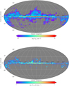Fig. 3

Comparison between $N_{H_{2}}$ ${N_{{{\rm{H}}_2}}}$ and W_CO maps. Top panel: Mollweide projection of our $N_{H_{2}}$ ${N_{{{\rm{H}}_2}}}$ map. The dark blue color indicates regions with $19 ≲ \log N_{H_{2}} ({cm}^{- 2}) ≲ 20$ $19 \mathbin{\lower.3ex\hbox{$\buildrel<\over {\smash{\scriptstyle\sim}\vphantom{_x}}$}} \log {N_{{{\rm{H}}_2}}}\left( {{\rm{c}}{{\rm{m}}^{ - 2}}} \right) \mathbin{\lower.3ex\hbox{$\buildrel<\over {\smash{\scriptstyle\sim}\vphantom{_x}}$}} 20$ . Bottom panel: W_CO map from Dame et al. (2001). Our $N_{H_{2}}$ ${N_{{{\rm{H}}_2}}}$ map was constructed by calculating A_V(H₂), using E(B − V) and N_H I data, and then converting to $N_{H_{2}}$ ${N_{{{\rm{H}}_2}}}$ using the relation given in Eq. (7). The $N_{H_{2}}$ ${N_{{{\rm{H}}_2}}}$ map shows several relatively large angular scale structures. As these are CO-dark H₂ regions, they are undetectable in the W_CO map. (Sect. 5.2). In both maps, longitude increases to the left from the central (vertical) line at ℓ = 0°, the grid spacing, shown by the white solid lines, is 30°, the angular resolution is 16′, and the HEALPix parameter NSIDE = 1024.

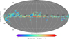Fig. 4

Mollweide projection of our constructed X_CO map. Our global value for X_CO is 2 × 10²⁰ K km s⁻¹ cm⁻², which is consistent with previous estimates. X_CO varies by orders of magnitude within a few tens of arcminutes. In the surroundings of molecular regions, X_CO ~ 10²¹ cm⁻² (K km s⁻¹)⁻¹, while in the inner parts of clouds it decreases to X_CO ~ 5 × 10¹⁹ cm⁻² (K km s⁻¹)⁻¹. In the Galactic center, X_CO increases significantly due to the high optical depths in that region. The angular resolution is 16′, and NSIDE=1024.

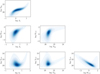Fig. 5

2D probability density functions relating the different parameters studied in this work (Sect. 4.1).

4.2 Comparison to the N_H₂ map of Kalberla et al. (2020)

Kalberla et al. (2020) used the nonlinear deviations in the E(B − V)−N_H I relation to estimate $N_{H_{2}}$ ${N_{{{\rm{H}}_2}}}$ . Our method is similar to that of Kalberla et al. (2020), although with some key differences that we discuss below.

4.2.1 Summary of the Kalberla et al. (2020) method

H I emits at various Doppler-shifted frequencies (velocities). Each velocity component is considered to be a distinct cloud along the LOS. Kalberla et al. (2020) decomposed the H I emission spectra into distinct Gaussian components³. Each Gaussian is characterized by an amplitude and a dispersion: the amplitude is proportional to the total H I emitting gas, while the spread (σ_u) represents the internal velocity dispersion of the H I gas, consisting of a thermal and turbulent component.

Kalberla et al. (2020) assigned an effective temperature (T_D) – in their paper this is referred to as the Doppler temperature – to each decomposed Gaussian component, where T_D represents the total width of the Gaussian component. They calculated the dust extinction expected from each H I Gaussian component, by assuming a constant dust-to-gas ratio (Lenz et al. 2017). Then, they added the E(B − V) contribution from all Gaussian components to estimate the total dust extinction induced by dust mixed with H I gas. They compared their estimated H I based extinction to the total extinction, using the map of Schlegel et al. (1998), and attributed the residuals to the presence of molecular gas.

4.2.2 Similarities and differences with our method

The similarities between our method and that of Kalberla et al. (2020) are the following: (1) both methods rely on the assumption of a universal dust-to-gas ratio and on the hypothesis that nonlinear deviations in the E(B − V)N_H I relation trace the molecular gas content. (2) Both methods employ a mapping function that converts the E(B − V)N_H I nonlinearities to $N_{H_{2}}$ ${N_{{{\rm{H}}_2}}}$ .

The major difference between our method and that of Kalberla et al. (2020) lies on how the mapping function was obtained. Kalberla et al. (2020) derived their mapping function by minimizing the extinction nonlinearities from the linear relation through bootstrapping. We derived our mapping function from independent data by using $N_{H_{2}}$ ${N_{{{\rm{H}}_2}}}$ measurements from UV spectra of background objects (Sect. 2). In addition, Kalberla et al. (2020) fitted their calibration function in regions where CO is undetectable. In CO-emitting regions, they estimated $N_{H_{2}}$ ${N_{{{\rm{H}}_2}}}$ by assuming a constant X_CO. On the other hand, our method does not require any assumption concerning X_CO. Finally, we note that Kalberla et al. (2020) decomposed the H I components based on their spread (T_D), while we treated all the H I components uniformly.

4.2.3 Comparison of the maps

Figure 6 shows the $N_{H_{2}}$ ${N_{{{\rm{H}}_2}}}$ map of Kalberla et al. (2020) together with our map at 2° resolution. We only include regions with log $N_{H_{2}} ({cm}^{- 2}) \geq 20$ ${N_{{{\rm{H}}_{\rm{2}}}}}\left( {{\rm{c}}{{\rm{m}}^{ - 2}}} \right) \ge 20$ , because below that threshold both methods might be susceptible to noise artifacts.

The $N_{H_{2}}$ ${N_{{{\rm{H}}_2}}}$ structures are more extended in the map of Kalberla et al. (2020) than ours. This difference could be due to degeneracies in the definition of T_D, which consists of a nonthermal (turbulent) and thermal component. The method of Kalberla et al. (2020) employs T_D as a proxy for the gas kinetic temperature, which is correlated with the molecular abundance. This approximation is accurate because the distribution of sonic Mach numbers in the diffuse ISM has a well-defined peak⁴ (Heiles & Troland 2003b). Although T_D represents the average gas temperature in the diffuse ISM, deviations toward individual regions are inevitably present.

We define the difference in the column densities of our map and the map of Kalberla et al. (2020) as $Δ (\log N_{H_{2}}) = \log N_{H_{2}}^{here} - \log N_{H_{2}}^{Kalberla+2020} .$ ${\rm{\Delta }}\left( {\log {N_{{{\rm{H}}_2}}}} \right) = \log N_{{{\rm{H}}_2}}^{{\rm{here}}} - \log N_{{{\rm{H}}_2}}^{{\rm{Kalberla + 2020}}}.$ (8)

Figure 7 shows a full-sky map of $Δ (\log N_{H_{2}})$ $\Delta \left( {\log {N_{{{\rm{H}}_{\rm{2}}}}}} \right)$ , calculated only in regions where both maps yield $N_{H_{2}} \geq 10^{20} {cm}^{- 2}$ ${N_{{{\rm{H}}_{\rm{2}}}}} \ge {10^{20}}\,\,{\rm{c}}{{\rm{m}}^{ - 2}}$ . The majority of the pixels have $Δ (\log N_{H_{2}}) < 0$ $\Delta \left( {\log {N_{{{\rm{H}}_{\rm{2}}}}}} \right) < 0$ , while in the Galactic plane we find that $Δ (\log N_{H_{2}}) > 0$ $\Delta \left( {\log {N_{{{\rm{H}}_{\rm{2}}}}}} \right) > 0$ .

We focus on Galactic latitudes |b| ≥ 10^°, because typical extinctions in the Galactic plane exceed the A_V range used for the calibration of the two methods. Figure 8 shows the distribution of $Δ (\log N_{H_{2}})$ $\Delta \left( {\log {N_{{{\rm{H}}_2}}}} \right)$ of all pixels at |b| ≥ 10°. The distribution peaks at −0.5, which implies that the $N_{H_{2}}$ ${N_{{{\rm{H}}_2}}}$ estimates in the map of Kalberla et al. (2020) are, on average, ~3 times larger than ours. Their estimates are consistent within the uncertainties of our method (Sect. 2.4).

The method of Kalberla et al. (2020) was calibrated in CO-dark H₂ regions, while in CO-bright regions they estimated $N_{H_{2}}$ ${N_{{{\rm{H}}_2}}}$ by assuming that X_CO = 4 × 10²⁰ cm⁻² (K km s⁻¹)⁻¹. Although this value is consistent with the range of local X_CO variations, 1.7−4.1 × 10²⁰ cm⁻² (K km s⁻¹ it is a factor of 2 larger than the Galactic average (Bolatto et al. 2013). If Kalberla et al. (2020) had adopted the global value of X_CO, then our estimates would differ, on average, by less than a factor of 2. A careful visual comparison of the $Δ (\log N_{H_{2}})$ $\Delta \left( {\log {N_{{{\rm{H}}_2}}}} \right)$ (Fig. 7) and the W_CO map (Fig. 3, bottom panel) shows that the $N_{H_{2}}$ ${N_{{{\rm{H}}_2}}}$ estimates of the two methods agree well, $Δ (\log N_{H_{2}}) \approx 0$ $\Delta \left( {\log {N_{{{\rm{H}}_2}}}} \right) \approx 0$ , in regions where CO is undetected.

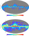Fig. 6

$N_{H_{2}}$ ${N_{{{\rm{H}}_2}}}$ map constructed using the method presented here (upper panel) and using that in Kalberla et al. (2020; lower panel). The resolution of both maps is 2° and NSIDE = 1024.

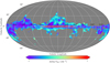Fig. 7

Difference between our $N_{H_{2}}$ ${N_{{{\rm{H}}_2}}}$ estimates and those of Kalberla et al. (2020).

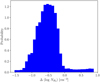Fig. 8

Distribution of the difference (our Eq. (8)) of our $N_{H_{2}}$ ${N_{{{\rm{H}}_2}}}$ estimates and those of Kalberla et al. (2020) for regions with |b| ≥ 10°. Our $N_{H_{2}}$ ${N_{{{\rm{H}}_2}}}$ estimates are, on average, three times smaller than those inferred by Kalberla et al. (2020). This difference likely results in large part from the X_CO value employed in the method of Kalberla et al. (2020).

5 Characterization of the total gas properties of our Galaxy

Characterizing the total gas properties of our Galaxy is an important but challenging task. It is hard to constrain $N_{H_{2}}$ ${N_{{{\rm{H}}_2}}}$ , which is usually estimated using CO observations by assuming some global (and constant) X_CO value. However, X_CO varies by orders of magnitude between the various regions (Sect. 4.1), and in addition a significant portion of the molecular gas lies in diffuse clouds that are largely devoid of CO (CO-dark H₂).

Dust traces the total hydrogen column density, including atomic and molecular in either CO-dark or CO-bright form. For the NH₂ estimate, we employed the nonlinearities in the dust extinction (Sect. 2). Thus, our $N_{H_{2}}$ ${N_{{{\rm{H}}_2}}}$ map (Fig. 3) probes the total H₂ column (CO-dark and CO-bright), which enables us to explore the various gas properties irrespective of the gas phase (atomic or molecular, CO-dark or CO-bright H₂). In the following sections, we use our constructed $N_{H_{2}}$ ${N_{{{\rm{H}}_2}}}$ map to explore the relative abundances between H I and H₂ gas, and we constrain the sky distribution of CO-dark and CO-bright H₂.

5.1 Relative abundance of atomic and molecular gas

The molecular fractional abundance $(f_{H_{2}})$ $\left( {{f_{{{\rm{H}}_2}}}} \right)$ is defined as $f_{H_{2}} = \frac{2 N_{H_{2}}}{N_{HI} + 2 N_{H_{2}}} .$ ${f_{{{\rm{H}}_2}}} = {{2{N_{{{\rm{H}}_2}}}} \over {{N_{{\rm{HI}}}} + 2{N_{{{\rm{H}}_2}}}}}.$ (9)

When $f_{H_{2}} \to 0$ ${f_{{{\rm{H}}_2}}} \to 0$ , then the total gas column is mostly in atomic form, while when $f_{H_{2}} \to 1$ ${f_{{{\rm{H}}_2}}} \to 1$ gas is 100% molecular.

Some fraction of the dust is expected to be mixed with ionized hydrogen, which is omitted in Eq. (9). The contribution of H+ in dust extinction, if any, is only expected in low-extinction regions (A_V ≲0.093 mag, Liszt 2014a). However, this is below the extinction range where our method is applicable, which is $\log N_{H_{2}} \geq 19$ $\log {N_{{{\rm{H}}_2}}} \ge 19$ (Fig. 1) or log A_v ≥ −0.5 (Fig. 2). Thus, we expect that our estimated $f_{H_{2}}$ ${{\rm{f}}_{{{\rm{H}}_2}}}$ remains statistically unchanged even if some ionized hydrogen is present.

We used the $N_{H_{2}}$ ${N_{{{\rm{H}}_2}}}.$ values from the map we constructed (Fig. 3, upper panel) and the N_{h i} data from the HI4PI survey to construct a full-sky $F_{H_{2}}$ ${F_{{{\rm{H}}_2}}}$ map (Fig. 9). We observe that close to the Galactic center (ℓ ≲ 60° and ℓ ≳ 300°, b = 0°), gas tends to be fully molecular. On the other hand, $F_{H_{2}}$ ${F_{{{\rm{H}}_2}}}$ dramatically decreases in the outer parts of the Galactic plane (300° ≳ℓ≳ 60°, b = 0°), meaning that the relative abundance of H I increases.

The $F_{H_{2}}$ ${F_{{{\rm{H}}_2}}}$ full-sky map also shows several large-scale structures above the Galactic plane with enhanced molecular abundances $(\log f_{H_{2}} ≳ 0.5)$ $\left( {\log {f_{{{\rm{H}}_2}}} \mathbin{\lower.3ex\hbox{$\buildrel>\over {\smash{\scriptstyle\sim}\vphantom{_x}}$}} 0.5} \right)$ : (1) the Taurus molecular cloud at ℓ, b ~ 170° – 15°, (2) the Polaris Flare at ℓ, b ~ 125°, 30°, (3) the North Polar Spur at ℓ, b ~ 27°, 10°, and (4) Orion at ℓ, b ~ 170°, −15°. Below we argue that the proximity of these molecular structures imply that the scale height of $N_{H_{2}}$ ${N_{{{\rm{H}}_2}}}$ of our Galaxy should be less than 300 pc.

Zucker et al. (2021) used the 3D extinction map of Leike et al. (2020) to derive the distances of Taurus and Orion, which are close to 150 and 400 pc, respectively. The distance estimates to the Polaris Flare are more uncertain, ranging from 100 pc up to 400 pc (Heithausen & Thaddeus 1990; Zagury et al. 1999; Brunt 2003; Schlafly et al. 2014; Panopoulou et al. 2016). The North Polar Spur is a gigantic radio loop and there is a debate regarding its distance. Some Galactic models suggest that this structure is a few kiloparsecs away from the Sun. However, recently Panopoulou et al. (2021) compared submillimeter and radio polarization data and found that the maximum distance of the North Polar Spur is approximately equal to 400 pc from the Sun. Altogether, all the aforementioned large-scale H₂ structures above the Galactic plane are relatively close to the Sun.

To be conservative, we assume that the maximum distance of the aforementioned molecular clouds is 500 pc. Assuming that b = 45°, which is the maximum Galactic Latitude where molecular clouds are observed in Fig. 3, we obtain a vertical distance from the Galactic plane equal to 350 pc. This distance barely exceeds the outer edge of the Local Bubble (Pelgrims et al. 2020). Therefore, most of the H₂ gas of our Galaxy lies within a vertical distance of 350 pc of the Galactic plane. This is consistent with previous constraints of the H₂ scale height of our Galaxy (Heyer & Dame 2015; Marasco et al. 2017).

Figure 10 shows the distribution of the logarithm of $F_{H_{2}}$ ${F_{{{\rm{H}}_2}}}$ . The distribution is nearly symmetric with an average equal to $〈 f_{H_{2}} 〉 \approx 25 %$ $\left\langle {{f_{{{\rm{H}}_2}}}} \right\rangle \approx 25\%$ , which is consistent with previous constraints derived with UV spectra of sparsely located point sources (Shull et al. 2021). From the cumulative distribution function of $F_{H_{2}}$ ${F_{{{\rm{H}}_2}}}$ , shown in Fig. 11, we calculate that a large fraction (80%) of our Galaxy with $N_{H_{2}} \geq 10^{20} {cm}^{- 2} has f_{H_{2}} ≲ 40 %$ ${N_{{{\rm{H}}_2}}} \ge {10^{20}}{\rm{c}}{{\rm{m}}^{ - 2}}{\rm{ has }}{f_{{{\rm{H}}_2}}} \mathbin{\lower.3ex\hbox{$\buildrel<\over {\smash{\scriptstyle>}\vphantom{_x}}$}} 40\%$ . This indicates that either the majority of the molecular gas of our Galaxy lies in diffuse molecular clouds or that atomic clouds are more abundant than molecular clouds. Below we argue that the latter is more probable.

We display $f_{H_{2}}$ ${F_{{{\rm{H}}_2}}}$ versus A_v in Fig. 12. For −0.5 ≲ log A_v ≲ −0.2, $\log f_{H_{2}}$ $\log {f_{{{\rm{H}}_2}}}$ increases from −2.0 (1% ) to −0.5 (30%), because the atomic gas transitions to molecular in this range of extinction, given an ambient radiation field of ~1 Habing. The observed nonlinear increase in $F_{H_{2}}$ ${F_{{{\rm{H}}_2}}}$ , is similar to the predicted behavior of semi-analytical models of the H I → H₂ transition (Draine & Bertoldi 1996; Krumholz et al. 2008, 2009; McKee & Krumholz 2010; Sternberg et al. 2014, 2024; Bialy & Sternberg 2016). For −0.2 ≲ log A_v ≲ 0.7, we observe that $\log f_{H_{2}}$ $\log {f_{{{\rm{H}}_2}}}$ slightly decreases from −0.5 (30%) to −0.7 (20%). Although A_v increases by a factor of 5, $F_{H_{2}}$ ${F_{{{\rm{H}}_2}}}$ decreases by a factor of 1.5. This suppression of $F_{H_{2}}$ ${F_{{{\rm{H}}_2}}}$ could be due to young stars that are illuminating the surrounding material and hence responsible for photo-destruction of the molecular gas (Madden et al. 2020). We consider this scenario unlikely because the decline of $F_{H_{2}}$ ${F_{{{\rm{H}}_2}}}$ starts at A_v ≈ 1 mag, which is typical of translucent (non-star-forming) clouds, such as the Polaris Flare.

We conclude simply that there are more atomic than molecular clouds in most of the LOSs of our Galaxy, even where we observe molecular gas. The concatenation of atomic clouds increases N_{H I} and consequently A_v, but not $N_{H_{2}}$ ${N_{{{\rm{H}}_2}}}$ ; hence, the reduction in $F_{H_{2}}$ ${F_{{{\rm{H}}_2}}}$ .

This suppression of $F_{H_{2}}$ ${F_{{{\rm{H}}_2}}}$ is more prominent close to the Galactic plane: the majority of LOSs with $\log f_{H_{2}} \approx - 1$ $\log {f_{{{\rm{H}}_2}}} \approx - 1$ and log A_v ≈ 0.7 are observed at \b\ ≈ 5°. However, even in regions at high Galactic latitudes (\b\ > 40°), which cover a large portion of the sky, we observed a similar trend. For \b\ > 40°, there are several LOSs with $\log f_{H_{2}} \approx - 0.5$ $\log {f_{{{\rm{H}}_2}}} \approx - 0.5$ and log A_v ≈ 0.

This suppression is expected from the following approximate calculation. The average number of atomic clouds per LOS, as indicated by H I emission line data, is close to three for \b\ > 40° (Panopoulou & Lenz 2020). On the other hand, the number of molecular clouds per LOS is a maximum two because: (1) molecular gas is associated with the H I cloud having an exceptionally large column, usually observed in H I emission data at low velocities measured with respect to the local standard of rest, and (2) molecular gas associated with H I clouds at intermediate local-standard-of-rest velocities tend to have lower column densities than clouds with lower velocities and only occasionally show any sign of H₂ (e.g., Lenz et al. 2015; Röhser et al. 2016a,b). Thus, we expect the ratio of the number of molecular clouds to atomic clouds to be a maximum of ≈0.67, implying that the high-Galactic-latitude sky has more atomic than molecular clouds. The majority of LOSs with $\log f_{H_{2}} \approx 0$ $\log {f_{{{\rm{H}}_2}}} \approx 0$ and log A_v ≳ 0.7 are toward the Galactic midplane (ℓ ≲ 30° and ℓ ≳ 330°, b = 0°).

Our conclusion about the decrease in $f_{H_{2}}$ ${F_{{{\rm{H}}_2}}}$ at high A_v is also evident in Fig. 20 of Planck Collaboration XXIV (2011). These authors compare $N_{H_{2}}$ ${N_{{{\rm{H}}_2}}}$ measurements used for the computation of $f_{H_{2}}$ ${F_{{{\rm{H}}_2}}}$ have been obtained from UV spectra (Rachford et al. 2002, 2009; Gillmon et al. 2006; Wakker 2006). This suggests that despite the significant beam difference (16' in our study, and pencil beams for the UV data), the observed trend is robust. The concatenation of multiple clouds along the LOS can significantly complicate observational studies of the HI → H₂ transition (Browning et al. 2003).

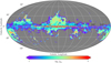Fig. 9

All-sky image of the logarithm of the fractional H₂ abundance, $f_{H_{2}}$ ${{\rm{f}}_{{{\rm{H}}_2}}}$ . The mean value of $\log f_{H_{2}}$ $\log {f_{{{\rm{H}}_2}}}$ is equal to −0.6, with standard deviation equal to 0.23.

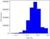Fig. 10

Distribution of values of the H₂ fractional abundance. Our mean $f_{H_{2}} = 0.25$ ${f_{{{\rm{H}}_2}}} = 0.25$ (with lσ range in linear scale 0.15–0.43) is consistent with Liszt & Gerin (2023), and Shull et al. (2021), who found the average $F_{H_{2}}$ ${F_{{{\rm{H}}_2}}}$ to be 0.2–0.4 and 0.20, respectively.

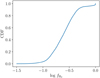Fig. 11

Cumulative distribution function of $F_{H_{2}}$ ${F_{{{\rm{H}}_2}}}$ . Atomic hydrogen is more abundant than molecular: 50%, and 80% of the LOSs have $f_{H_{2}} ≲ 25 %, and f_{H_{2}} ≲ 40 %,$ ${f_{{{\rm{H}}_2}}} \mathbin{\lower.3ex\hbox{$\buildrel<\over {\smash{\scriptstyle\sim}\vphantom{_x}}$}} 25\% {\rm{, and }}{f_{{{\rm{H}}_2}}} \mathbin{\lower.3ex\hbox{$\buildrel<\over {\smash{\scriptstyle\sim}\vphantom{_x}}$}} 40\% {\rm{, }}$ , respectively, while only −3% have $f_{H_{2}} \geq 80 %$ ${f_{{{\rm{H}}_2}}} \ge 80\%$ .

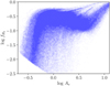Fig. 12

Molecular fractional abundance as a function of dust extinction. The nonlinear increase in $F_{H_{2}}$ ${F_{{{\rm{H}}_2}}}$ at −0.5 ≲ log A_v (mag) ≲ −0.2 corresponds to the atomic to molecular gas transition. At larger A_v, $F_{H_{2}}$ ${F_{{{\rm{H}}_2}}}$ decreases by a factor of 1.5, most probably because even along high-extinction sightlines there exist more atomic than molecular clouds.

5.2 The properties of CO-dark and CO-bright H₂

There is a significant fraction of molecular gas that is not traced by CO. This CO-dark H₂ is observed in diffuse ISM clouds where the H I → H₂ transition is ongoing. In regions where the HI → H₂ transition is well advanced, carbon monoxide formation can also occur. Between the extinctions that characterize the predominance of H₂ and CO, carbon transitions from C⁺ to C I. For typical ISM conditions, the onset of the H₂ formation takes place at A_v ≲ 0.5 mag, the C⁺ → C I transition at 1 ≲ A_v ≲ 3 mag, while CO becomes the dominant carrier of carbon at A_v ≥ 3 mag. During the transition from C⁺ to C I, H₂, whose electronic transitions due to photon absorption (Lyman-Werner lines) start at 11.18 eV, has already started forming but carbon is still in atomic form. Sufficient shielding is required to reduce the energy of incident photons below the CO photo-dissociation threshold (11.09 eV), hence allowing the buildup of the abundance of CO. Until this energy threshold is reached, the H₂ absorption lines are detectable but without any corresponding CO emission line. In this case, molecular hydrogen is primarily mixed with atomic carbon.

The integrated intensity of the [C II] line (at 158 μm) is proportional to the gas density squared (Goldsmith et al. 2018) at the densities characteristic of diffuse and translucent clouds. Toward several clouds with untraceable CO, the observed [C II] intensity, even assuming all carbon is in the form of C⁺, is larger than that expected solely from C-H I collisions (Langer et al. 2010). The enhancement of the [C II] line indicates the presence of H₂ gas.

The above discussion makes it clear that our ability to trace CO-dark H₂ relies on the observational uncertainties in the CO line. Even in diffuse regions, there should be some CO emission, although very weak. Strictly speaking CO-dark H₂ is located in regions where the atomic carbon is more abundant than CO, or in terms of observables, when the [C ii] or [C i] lines are stronger than CO. In this work, we adopt a detectability threshold of the CO line in order to define CO-dark H₂. The detectability limit is determined by the noise in the CO data of Dame et al. (2001), which is 1 K km s^-1.

We adopt the definition that molecular gas is in CO-dark form when the following conditions are satisfied: (1) $\log N_{H_{2}} \geq 19 {cm}^{- 2}$ $\log {N_{{{\rm{H}}_2}}} \ge 19{\rm{c}}{{\rm{m}}^{ - 2}}$ , and (2) W_CO ≤ 1 Kkm s^-1. On the other hand, we define molecular gas that is traceable by CO, CO-bright H₂, as: (1) $\log N_{H_{2}} \geq 19 {cm}^{- 2}$ $\log {N_{{{\rm{H}}_2}}} \ge 19{\rm{c}}{{\rm{m}}^{ - 2}}$ and (2) W_CO > 1 K km s^-1.

Figure 13 shows our inferred CO-dark (upper panel), and CO-bright (lower panel) NH₂ maps. We observe that CO-dark H₂ extends to high Galactic latitudes (|b| ≈ 60°), and has generally lower column densities than CO-bright H₂, because CO-dark H₂ is characteristic of regions having lower densities than CO-bright H₂. CO-dark H₂ increases toward lower Galactic Latitudes, but in the Galactic plane almost all of the molecular gas is in CO-bright form due to the enhanced densities, and column densities there. CO-bright H₂ lies close to the Galactic plane and only a few CO-emitting clouds can be seen at higher latitudes (|b| ≈ 30°).

We estimate that CO-dark H₂ covers ~17% of the total sky area, while CO-bright H₂ ~9% of the sky. These values, however, should be considered with some caution because the W_CO map of Dame et al. (2001) is considered to be complete only for |b| ≤ 32°, as indicated by the comparison between the CO intensities with far-infrared and H I data⁵. Thus, the W_CO map may miss some CO emission at high Galactic latitudes (|b| > 32°), although we do not expect the emission at such high b to be significant. Our argument is supported by the CO survey of Dame & Thaddeus (2022), which is complete for the entire northern sky, and shows that very few LOSs have detectable CO emission - assuming the sensitivity of the Dame et al. (2001) survey – at |b| > 40°. Therefore, our inferred fractional sky coverage of the CO-dark, and CO-bright H₂ components should be considered as upper and lower limits, respectively. Finally, we find that 66% of the sightlines with log $N_{H_{2}} ({cm}^{- 2}) \geq 19$ ${N_{{{\rm{H}}_2}}}\left( {{\rm{c}}{{\rm{m}}^{ - 2}}} \right) \ge 19$ are in CO-dark form, while the remaining 34% of sightlines are in CO-bright form. If in the definition of CO-dark H₂ we increase the threshold to log $N_{H_{2}} ({cm}^{- 2}) \geq 20$ ${N_{{{\rm{H}}_2}}}\left( {{\rm{c}}{{\rm{m}}^{ - 2}}} \right) \ge 20$ , we obtain that 57% of the LOSs are in CO-dark and 43% in CO-bright form.

6 Dust-to-gas ratio

N_H/E(B − V) is a key ratio for ISM studies. Existing constraints on the Galactic average N_H/E(B – V) vary significantly (Liszt & Gerin 2023). The constraint of Bohlin et al. (1978), N_H/E(B – V) = 5.8 × 10²¹ cm^-2 mag^-1, has been the gold standard for several decades. But, several recent works (Lenz et al. 2017; Planck Collaboration XI 2014; Shull et al. 2021; Liszt & Gerin 2023; Liszt 2014a; Gillmon et al. 2006; Rachford et al. 2009) have found larger values, although Kalberla et al. (2020) quote a smaller value for the Galactic average of N_H/E(B – V). However, when Kalberla et al. (2020) excluded regions close to the Galactic plane, they found a larger value than Bohlin et al. (1978).

Variations in the N_H /E(B – V) ratio can be induced by different factors: (1) environmental ISM conditions (Paradis et al. 2012), (2) dynamical effects (e.g., imperfect coupling between dust and gas motions, Squire & Hopkins 2018; Hopkins & Squire 2018; Hopkins et al. 2020, 2022), and (3) the V-band could be less than optimal for measuring dust extinction (Jura 1980; Butler & Salim 2021).

Atomic clouds at high Galactic Latitudes, where N_H ≈ N_{H i}, have larger dust-to-gas ratio, N_H/E(B – V) = 8–10 × 10²¹ cm^-2 mag^-1 (Liszt 2014b; Lenz et al. 2017), than the Galactic plane, where N_H/E(B – V) lies in the range 5.8–6.1 × 10²¹ cm^-2 mag^-1 (Bohlin et al. 1978; Rachford et al. 2002, 2009; Shull et al. 2021). Uncertainties in the employed techniques (UV or radio spectroscopy, far-infrared dust emission) could also induce variations in the constrained N_H/E(B – V) (Shull & Panopoulou 2023).

The only direct way to constrain N_H, and hence the dust-to-gas ratio, is by the use of spectra of background objects (e.g., Bohlin et al. 1978; Sheffer et al. 2008; Gillmon et al. 2006; Rachford et al. 2009; Shull et al. 2021). However, obtaining spectra is time consuming and only a limited number of LOSs can be targeted, usually toward relatively bright stars and quasars. The sky is sparsely sampled, which implies that the N_H/E(B – V) estimates could be biased as spectroscopic surveys usually focus on the Galactic plane. Indirect methods for constraining the dust-to-gas ratio require some assumptions and approximations, but they have the advantage of uniformly sampling the Galaxy (Paradis et al. 2012; Planck Collaboration XIX 2011; Planck Collaboration XI 2014; Kalberla et al. 2020).

In Fig. 14, we present our N_H/E(B – V) constraint and compare it to previous work. The figure shows the total hydrogen column density, calculated as $N_{H} = N_{H 1} + 2 N_{H_{2}}$ ${N_{\rm{H}}} = {N_{{\rm{H}}1}} + 2{N_{{{\rm{H}}_2}}}$ , including data covering the full celestial sphere; the data employed are the N_{H i} full-sky map from HI4PI Collaboration (2016), and our constructed $N_{H_{2}}$ ${N_{{{\rm{H}}_2}}}$ map (Fig. 3). The colored dashed lines correspond to previous constraints.

All the depicted lines are consistent, within variations, with our data. However, the green and red lines, which correspond to 7.0 × 10²¹ cm^-2 mag^-1 (Planck Collaboration XI 2014) and 5.8 × 10²¹ cm^-2 mag^-1 (Bohlin et al. 1978), respectively, agree more closely with the mean behavior of our data.

We can approximate, to first order, the N_H versus E(B - V) relation with a line. But, a closer inspection to Fig. 14 suggests that some nonlinearities arise. For E(B – V) ≤ 0.1 mag, the average behavior of our data agrees well with the green line describing the results of Planck Collaboration XI (2014), while for E(B – V) > 0.1 mag the red profile of Bohlin et al. (1978) seems to be a better fit. This indicates that at larger E(B - V) the dust-to-gas ratio decreases, which could happen due to dust coagulation.

7 Discussion

7.1 A historical perspective on the extinction residuals

Boulanger et al. (1996) found that dust intensity correlates with the HI integrated intensity (W_Hi). The correlation is linear for W_{H I} ≤ 300 K km s^-1 and nonlinear for W_{H I} > 300 K km s^-1. Assuming that the H I line is optically thin the H I column density is given by N_{h i} = 1.823 ×10¹⁸ W_{h i} (Draine 2011), yielding a transition at N_HI ≈ 5 × 10²⁰ cm^-2. Boulanger et al. (1996) argued that the nonlinear excess between dust intensity and W_{h i} is due to the presence of molecular gas that is only probed by dust intensity, which traces both the atomic and molecular gas phase, while the 21 cm emission line probes only the atomic phase. Their argument was based on the results of Savage et al. (1977), who found, using the H₂ absorption lines, that the molecular gas fraction rapidly increases when N_HI ≈ 5 × 10²⁰ cm^-2. An alternative explanation of the nonlinear relationship between dust intensity and W_H I for W_H I > 300 K km s^-1 is that at some point the emission line becomes optical thick and W_{h i} misses a significant faction of the H I due to self-absorption, and reduction of the observed intensity (Burton et al. 1992).

The same debate is found in more recent papers. Fukui et al. (2014, 2015) explored the correlation between W_{h i} and the dust opacity (t₃₅₃), but they also added one more free parameter in the analysis: the dust temperature (T_d). The dust temperature is anticorrelated with the total gas column. Warm dust traces the outer regions of iSM clouds, which are primarily atomic, while cold dust traces the inner, primarily molecular, regions of the clouds. Fukui et al. (2015) showed that the correlation between W_H I and t₃₅₃ is linear when T_d > 20 K. When dust is cold (T_d < 20 K), t₃₅₃ increases nonlinearly with respect to W_H I. Fukui et al. (2015) argued that this nonlinear excess of t₃₅₃ with respect to W_{h i} is consistent with the presence of optically thick H I gas, and although some H₂ gas might be present, it is less abundant than H I. At sufficiently high column densities, the increase in t₃₅₃ would be dominated by the formation of the molecular gas, which is traceable by the CO emission line. However, Fukui et al. (2015) suggest that the excess of τ₃₅₃ at low W_{h i} is not due to CO-dark H₂, but due to optically thick H I.

Murray et al. (2018) addressed the question of whether the Hi optical depth effects can explain the excess of τ₃₅₃ when W_{h i} is high. They compiled a large catalogue of t_H I absorption data, which provide the only direct way to estimate t_H I. Their sample consisted of archival data toward 151 LOSs that are covered within the Galactic Arecibo L-band Feed Array (GALFA) HI survey footprint. Following the analysis of Fukui et al. (2015), Murray et al. (2018) found that as t_H I increases, the HI gas that is missed by the 21 cm emission line is less than a factor of 1.3; similar results have been found by Liszt (2019). This means that the increase in t_H I cannot adequately explain the nonlinear relation between W_{h i} and t₃₅₃.

We found that nonlinear deviations in the extinction with respect to N_HI correlate well with $N_{H_{2}}$ ${N_{{{\rm{H}}_2}}}$ . Our findings (Fig. 1) support the claims of Boulanger et al. (1996), and Murray et al. (2018) - that extinction residuals are induced by molecular hydrogen. However, given the spread in our obtained A_v versus $N_{H_{2}}$ ${N_{{{\rm{H}}_2}}}$ relation (Fig. 1), some, but not dominant, contribution of optically thick HI gas is also plausible.

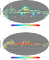Fig. 13

Comparison of the CO-dark and CO-bright $N_{H_{2}}$ ${N_{{{\rm{H}}_2}}}$ maps. Upper panel: full-sky CO-dark $N_{H_{2}}$ ${N_{{{\rm{H}}_2}}}$ map, showing sightlines with $N_{H_{2}} \geq 10^{19} {cm}^{- 2}$ ${N_{{{\rm{H}}_2}}} \ge {10^{19}}{\rm{c}}{{\rm{m}}^{ - 2}}$ cm^-2 but devoid of CO (W_CO < 1 Kkm s^-1). Bottom panel: CO-bright $N_{H_{2}}$ ${N_{{{\rm{H}}_2}}}$ map, corresponding to $N_{H_{2}} \geq 10^{19} {cm}^{- 2}$ ${N_{{{\rm{H}}_2}}} \ge {10^{19}}{\rm{c}}{{\rm{m}}^{ - 2}}$ cm^-2 and W_CO > 1 K km s^-1. The CO-dark H₂ spans an area approximately equal to 17% of the total sky. This is a factor of 2 larger than that of the CO-bright H₂, and extends up to high Galactic Latitude. On the other hand, CO-bright H₂ is mostly concentrated toward the Galactic plane. Moving away from the Galactic plane, we observe that H₂ transitions from CO-bright to CO-dark form at |b| ≈ 5 deg. Although we still observe a few CO-bright H₂ regions at higher latitudes above the Galactic plane, most of the molecular gas is in the CO-dark form there.

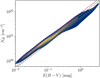Fig. 14

Total hydrogen column density versus dust reddening. The colored curves correspond to previously constrained dust-to-gas ratios. The blue, red, green, and magenta curves correspond to N_H/E(B – V) = 5.1 (Kalberla et al. 2020), 5.8 (Bohlin et al. 1978), 7.0 (Planck Collaboration XI 2014), and 8.8 (Lenz et al. 2017) x10²¹ cm^-2 mag^-1, respectively.

7.2 Variations in X_CO

The X_CO factor is an important observable for estimating the molecular gas content of molecular clouds and entire galaxies (Lee et al. 2014; Sun et al. 2018, 2020). XCO is expected to vary as a function of the local iSM properties, such as metallicity, density, and intensity of the UV background field (Gong et al. 2017, 2018). Observations of local iSM clouds suggest that the XCO factor is relatively constant, with variations not exceeding a factor of 2 (Bolatto et al. 2013; Liszt & Gerin 2016).

The constancy of X_CO indicates that iSM clouds in our Galaxy have generally similar properties, such as temperature and surface densities. This uniformity has important consequences regarding the nature of iSM clouds. For example, it explains the relation between nonthermal velocity linewidths and cloud size – known as Larson’s relation (Larson 1981) – as the outcome of clouds with magnetically supported boundaries (Mouschovias & Psaltis 1995). A plethora of theoretical works address the question of why ISM clouds in the Milky Way are so similar (e.g., Narayanan & Hopkins 2013; Clark & Glover 2015).

We have found that CO-emitting regions are most probably observed when $20.5 ≲ \log N_{H_{2}} ({cm}^{- 2}) ≲ 21$ $20.5 \mathbin{\lower.3ex\hbox{$\buildrel<\over {\smash{\scriptstyle\sim}\vphantom{_x}}$}} \log {N_{{{\rm{H}}_2}}}\left( {{\rm{c}}{{\rm{m}}^{ - 2}}} \right) \mathbin{\lower.3ex\hbox{$\buildrel<\over {\smash{\scriptstyle\sim}\vphantom{_x}}$}} 21$ , and 3 ≲ W_co ≲ 8 K km s^-1 (Fig. 5). Our results thus suggest, in agreement with previous studies, that our Galaxy favors clouds with relatively uniform CO and surface density properties. This is also supported by our inferred $f_{H_{2}}$ ${F_{{{\rm{H}}_2}}}$ distribution (Fig. 10), which is nearly symmetric and narrow; the 1 σ of the distribution is 0.15–0.43. However, in individual molecular clouds (on angular scales of a few arcminutes), X_CO can vary by an order of magnitude from the outer to the inner parts, as atomic gas transitions to fully molecular form.

7.3 Molecular hydrogen column densities as a function of the galactocentric distance

The Galactic plane contains most of the molecular gas of our Galaxy. Several authors employed data from the CO survey of Dame et al. (2001) to model the H₂ surface as a function of distance from the Galactic center, but omitted any contribution from CO-dark H₂ (Bronfman et al. 1988; Wouterloot et al. 1990; Nakanishi & Sofue 2006, 2016; Marasco et al. 2017; Miville-Deschenes et al. 2017).

A common conclusion from these works is that the H₂ surface density decreases nonlinearly at large galactocentric distances, although the different studies differ on the exact cutoff distance. It would be interesting to see how the effect of the CO-dark H₂ could affect the relative abundance between the HI and H₂ surface densities as a function of galactocentric distance. The presence of CO-dark H₂ could yield more extended H₂ surface density profiles, as shown by Pineda et al. (2013) who estimated that the H₂ gas in CO-dark form corresponds to ~20% of the total molecular abundance at 4 kpc and ~80% at 10 kpc.

Our $f_{H_{2}}$ ${F_{{{\rm{H}}_2}}}$ map (Fig. 9) shows that in the Galactic plane gas is mostly molecular for ℓ ≲ 60° and ℓ ≳ 300°, while it becomes fully atomic for 90° ≳ ℓ ≳ 270°. Despite the presence of CO-dark H₂, the overall contribution of molecular gas at large Galactic latitudes is minimal; the abundance of CO-dark H₂ becomes maximum at 150° ≳ ℓ ≳ 210°, but there $f_{H_{2}}$ ${F_{{{\rm{H}}_2}}}$ is only 10%. Thus, the CO-dark H₂ abundance seems to increase with galactocentric distance, but this only affects the exact distance where H I starts becoming more abundant than H₂.

7.4 CO-dark H₂ estimates in the solar neighborhood

Existing constraints on the relative abundance of CO-dark H₂ in relation to total gas imply that a significant amount of molecular gas exists in CO-dark form (Planck Collaboration XIX 2011; Paradis et al. 2012; Kalberla et al. 2020). As stated by Li et al. (2018), the derived abundances of CO-dark H₂ depend on the detectability threshold of the CO line. This was demonstrated by Donate & Magnani (2017) who performed a high-sensitivity CO survey toward a region with existing, lower sensitivity CO data. The (new) high-sensitivity survey showed that the relative abundance of CO-dark with respect to the total H₂ gas was approximately two times smaller than what had been inferred by the (previous) low-sensitivity CO survey. That said, the definition of CO-dark H₂ is vague, making the comparison of the various results in the literature challenging.

Our definition of CO-dark and CO-bright H₂ components differs from several past works (e.g., Paradis et al. 2012; Kalberla et al. 2020). In these works, the decomposition is based on the models of photo-dissociation regions (Wolfire et al. 2010; Velusamy et al. 2010). In photo-dissociation-region models, molecular gas phases are organized into layers with CO-dark corresponding to a diffuse, and hot layer that surrounds the dense, and cold CO-bright H₂ layer.

We define CO-dark H₂, molecular hydrogen in LOSs devoid of CO. Using this definition, CO-dark and CO-bright H₂ never coexist (Fig. 13). However, our definition allows us to emphasize that a significant fraction of the molecular sky (~60%) is untraceable in CO maps, when a detectability threshold equal to 1 K km s^-1 is employed (Sect. 5.2). Our estimates should be treated as upper limits, given the incompleteness of the Dame et al. (2001) CO survey at high Galactic latitudes. However, we do not expect significant variations from these estimates because CO emission is minimal in that portion of the Milky Way.

8 Conclusions

Molecular hydrogen is the most abundant molecule in the ISM, but it is hard to directly observe it and infer its column density. Several indirect methods have been used to probe $N_{H_{2}}$ ${N_{{{\rm{H}}_2}}}$ , usually by observing the CO emission lines and employing a CO–H₂ conversion factor (X_CO; Eq. (1)). However, CO misses the diffuse molecular hydrogen that lies in translucent clouds, where densities are not sufficient to allow a rapid formation of CO and column densities are insufficient to provide effective shielding against photo-dissociation.The result is CO-dark H₂. We present a new indirect method for estimating $N_{H_{2}}$ ${N_{{{\rm{H}}_2}}}$ using N_H I and dust extinction data.

We show that the nonlinear increments of dust extinction with respect to N_H I, A_V(H₂), observed for N_H I ≥ 3 × 10²⁰ cm^-2 (Lenz et al. 2017), are due to the presence of molecular hydrogen. We measure the implied extinction due to molecular hydrogen, A_V(H₂), using publicly available extinction maps (Green et al. 2019), toward LOSs with direct $N_{H_{2}}$ ${N_{{{\rm{H}}_2}}}$ measurements that have been obtained with spectroscopic data. We show that A_V(H₂) correlates with $N_{H_{2}}$ ${N_{{{\rm{H}}_2}}}$ (Fig. 1). We obtain a best-fit model for the $A_{V} (H_{2}) - N_{H_{2}}$ ${A_{\rm{V}}}\left( {{{\rm{H}}_2}} \right) - {N_{{{\rm{H}}_2}}}$ relation (Eq. (7)). The fitted relation is the basis of our methodology for estimating $N_{H_{2}}$ ${N_{{{\rm{H}}_2}}}$ .

We employed the following assumptions, which are motivated by the literature: (1) N_H/E (B – V) = 8.8 × 10²¹ cm^-2 mag^-1 (Lenz et al. 2017) and (2) R_v = 3.1 (Cardelli et al. 1989; Schlafly et al. 2014). We used the fitted relation (Eq. (7)) to construct a full-sky $N_{H_{2}}$ ${N_{{{\rm{H}}_2}}}$ map at 16' resolution (top panel in Fig. 3); our $N_{H_{2}}$ ${N_{{{\rm{H}}_2}}}$ map does not employ CO observations and hence traces both the CO-dark (diffuse) and CO-bright H₂. The accuracy of the obtained NH₂ estimates is better than a factor of 2, 3, and 5, with a probability of 68%, 95%, and 98%, respectively.

We compared our inferred NH₂ estimates with those of Kalberla et al. (2020) and find good agreement (Sect. 4.2); there is some discrepancy, which can be explained by the assumptions of the employed methods. We also compared our $N_{H_{2}}$ ${N_{{{\rm{H}}_2}}}$ map with the CO total intensity obtained from the composite survey of Dame et al. (2001) (our Sect. 4.1). We constructed a map of X_CO, which is the ratio between $N_{H_{2}}$ ${N_{{{\rm{H}}_2}}}$ and W_CO (Fig. 4). We estimate that the Galactic value of X_CO is approximately equal to 2 × 10²⁰ cm^-2 (K km s^-1)^-1, which is consistent with previous constraints (Bolatto et al. 2013; Lada & Dame 2020). However, we find that X_CO can vary by orders of magnitude on angular scales of a few arcminutes.

In the diffuse (peripheral) parts of ISM clouds, X_CO > 10²¹ cm^-2 (K km s^-1)^-1 because a large portion of the molecular hydrogen there is not traced by CO, hence the large conversion factor. On the other hand, in the inner (denser) parts of the cloud, where CO is well mixed with molecular hydrogen, X_CO decreases to −5 × 10¹⁹ cm^-2 (K km s^-1)^-1. Toward LOSs with A_V ≳ 10 mag - mostly encountered in the Galactic plane - the CO line saturates and X_co > 10²¹ cm^-2 (K km s^-1)^-1 (Fig. 5).

We used our $N_{H_{2}}$ ${N_{{{\rm{H}}_2}}}$ map and archival N_HI data to construct a map (Fig. 9) of the molecular fractional abundance $(f_{H_{2}}),$ $\left( {{f_{{{\rm{H}}_2}}}} \right),$ , which is the ratio between $N_{H_{2}}$ ${N_{{{\rm{H}}_2}}}$ and the total gas column (Eq. 9). For our Galaxy, we find an average $f_{H_{2}}$ ${F_{{{\rm{H}}_2}}}$ equal to 25% (Fig. 11), which is consistent with previous estimates (Bellomi et al. 2020; Shull et al. 2021). In the Galactic plane (b = 0°), for 90° ≲ ℓ ≲ 270°, $f_{H_{2}}$ ${F_{{{\rm{H}}_2}}}$ decreases abruptly from unity to 0.1. This agrees with previous constraints of the molecular gas distribution of our Galaxy (Miville-Deschenes et al. 2017; Marasco et al. 2017). We find that fH₂ approaches unity, implying that gas is fully molecular, only toward 3% of the LOSs with $N_{H_{2}} \geq 10^{20} {cm}^{- 2}$ ${N_{{{\rm{H}}_2}}} \ge {10^{20}}{\rm{c}}{{\rm{m}}^{ - 2}}$ . A large fraction of the sky (∽66%) with $N_{H_{2}} \geq 10^{19} {cm}^{- 2}$ ${N_{{{\rm{H}}_2}}} \ge {10^{19}}{\rm{c}}{{\rm{m}}^{ - 2}}$ is undetected in CO maps when the sensitivity of the CO data is W_CO = 1 K km s^-1 (Sect. 2).

We explored the correlation between N_H and E(B – V) (Sect. 6). Our data favor a N_H/E(B – V) ratio close to 7 × 10²¹ cm^-2 mag^-1 for E(B – V) ≲ 0.1 mag, consistent with the constraint of Planck Collaboration XI (2014). For E(B – V) ≲ 0.1 mag, our data fit better with the constraint of Bohlin et al. (1978), N_H/E(B – V) ≈ 5.8 × 10²¹ cm^-2 mag^-1. All the constructed maps are made publicly available through the Strasbourg astronomical Data Center.

Acknowledgements

We are grateful to the reviewer, J.M. Shull, for a very constructive report which significantly improved the manuscript. We would like to thank M. Heyer, P. Kalberla, K. Tassis, S. Stahler, and G. V. Panopoulou for useful comments on the draft and M. A. Miville-Deschenes, C. Murray, S. Bialy, A. Bracco, and B. Hensley for fruitful discussions. We also thank P. Kallemi for the graphic design in part of the figures. This work was supported by NSF grant AST-2109127. This work was performed in part at the Jet Propulsion Laboratory, California Institute of Technology, under contract with the National Aeronautics and Space Administration (80NM0018D0004). The authors acknowledge Interstellar Institute’s program "II6" and the Paris-Saclay University’s Institut Pascal for hosting discussions that nourished the development of the ideas behind this work.

Appendix A Full-sky $N_{H_{2}}$ ${N_{{{\bf{H}}_2}}}$ properties of our Galaxy using the Planck extinction map

We constructed a full-sky $N_{H_{2}}$ ${N_{{{\rm{H}}_2}}}$ map of our Galaxy using the extinction data of Planck Collaboration XII (2020) (Fig. A.1). We compared against the $N_{H_{2}}$ ${N_{{{\rm{H}}_2}}}$ map that we constructed with the extinction data of Schlegel et al. (1998) (Fig. 3).

Figure A.1 shows more extended $low- N_{H_{2}}$ ${\rm{ low - }}{N_{{{\rm{H}}_2}}}$ regions at high Galactic latitudes than Fig. 3. This happens because A_V in Planck Collaboration XII (2020) tends to be, overall, larger than in Schlegel et al. (1998). As we show below, the relatively enhanced A_V values of Planck Collaboration XII (2020) may affect some of the estimated molecular gas properties of our Galaxy.

We used the $N_{H_{2}}$ ${N_{{{\rm{H}}_2}}}$ data shown in Fig. A.1 to calculate the Galactic average X_CO and $f_{H_{2}}$ ${F_{{{\rm{H}}_2}}}$ . We obtain that 〈X_CO〉 ≈ 4 × 10²⁰ cm^-2 (K km s^-1)^-1, and $〈 f_{H_{2}} 〉 \approx 30 %$ $\left\langle {{f_{{{\rm{H}}_2}}}} \right\rangle \approx 30\%$ , which are ∽2 larger than what we inferred in Sects. 4.1, and 5, but both consistent with the range of values in the literature. In addition, the estimated sky fraction of CO-dark with respect to the total H₂ becomes ∽79%, while that of CO-bright ∽21% for LOSs with $N_{H_{2}} \geq 10^{20} {cm}^{- 2}$ ${N_{{{\rm{H}}_2}}} \ge {10^{20}}{\rm{c}}{{\rm{m}}^{ - 2}}$ . In this case the relative abundance of CO-dark H₂ is almost two times larger than what we get from the Schlegel et al. (1998) map (Sect. 5.2). We conclude that differences in the extinction maps can induce at most factor of 2 deviations in the estimated molecular hydrogen properties.

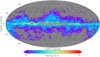Fig. A.1

Full-sky $N_{H_{2}}$ ${N_{{{\rm{H}}_2}}}$ map of our Galaxy constructed with the extinction map of Planck Collaboration XII (2020). Resolution and grid properties are the same as in Fig. 3.

References

André, P., Men’shchikov, A., Bontemps, S., et al. 2010, A&A, 518, L102 [Google Scholar]
Armus, L., Lai, T., U, V., et al. 2023, ApJ, 942, L37 [NASA ADS] [CrossRef] [Google Scholar]
Bailer-Jones, C. A. L., Rybizki, J., Fouesneau, M., Demleitner, M., & Andrae, R. 2021, AJ, 161, 147 [Google Scholar]
Barriault, L., Joncas, G., Lockman, F. J., & Martin, P. G. 2010, MNRAS, 407, 2645 [NASA ADS] [CrossRef] [Google Scholar]
Bellomi, E., Godard, B., Hennebelle, P., et al. 2020, A&A, 643, A36 [NASA ADS] [CrossRef] [EDP Sciences] [Google Scholar]
Bialy, S., & Sternberg, A. 2016, ApJ, 822, 83 [NASA ADS] [CrossRef] [Google Scholar]
Boccaletti, A., Lagage, P. O., Baudoz, P., et al. 2015, PASP, 127, 633 [CrossRef] [Google Scholar]
Bohlin, R. C., Savage, B. D., & Drake, J. F. 1978, ApJ, 224, 132 [Google Scholar]
Bolatto, A. D., Wolfire, M., & Leroy, A. K. 2013, ARA&A, 51, 207 [CrossRef] [Google Scholar]
Bouchet, P., García-Marín, M., Lagage, P. O., et al. 2015, PASP, 127, 612 [CrossRef] [Google Scholar]
Borchert, E. M. A., Walch, S., Seifried, D., et al. 2022, MNRAS, 510, 753 [Google Scholar]
Boulanger, F., Abergel, A., Bernard, J. P., et al. 1996, A&A, 312, 256 [Google Scholar]
Bronfman, L., Cohen, R. S., Alvarez, H., May, J., & Thaddeus, P. 1988, ApJ, 324, 248 [NASA ADS] [CrossRef] [Google Scholar]
Browning, M. K., Tumlinson, J., & Shull, J. M. 2003, ApJ, 582, 810 [NASA ADS] [CrossRef] [Google Scholar]
Brunt, C. M. 2003, ApJ, 584, 293 [NASA ADS] [CrossRef] [Google Scholar]
Burton, W. B., Elmegreen, B. G., Genzel, R., Pfenniger, D., & Bartholdi, P. 1992, ASP Conf. Ser., 31, 327 [Google Scholar]
Butler, R. E., & Salim, S. 2021, ApJ, 911, 40 [NASA ADS] [CrossRef] [Google Scholar]
Cardelli, J. A., Clayton, G. C., & Mathis, J. S. 1989, ApJ, 345, 245 [Google Scholar]
Cartledge, S. I. B., Lauroesch, J. T., Meyer, D. M., & Sofia, U. J. 2004, ApJ, 613, 1037 [NASA ADS] [CrossRef] [Google Scholar]
Clark, P. C., & Glover, S. C. O. 2015, MNRAS, 452, 2057 [NASA ADS] [CrossRef] [Google Scholar]
Cox, N. L. J., Arzoumanian, D., André, P., et al. 2016, A&A, 590, A110 [NASA ADS] [CrossRef] [EDP Sciences] [Google Scholar]
Dame, T. M., & Thaddeus, P. 2022, ApJS, 262, 5 [NASA ADS] [CrossRef] [Google Scholar]
Dame, T. M., Hartmann, D., & Thaddeus, P. 2001, ApJ, 547, 792 [Google Scholar]
Donate, E., & Magnani, L. 2017, MNRAS, 472, 3169 [CrossRef] [Google Scholar]
Draine, B. T. 2011, Physics of the Interstellar and Intergalactic Medium (Princeton University Press) [Google Scholar]
Draine, B. T., & Bertoldi, F. 1996, ApJ, 468, 269 [Google Scholar]
Draine, B. T., Dale, D. A., Bendo, G., et al. 2007, ApJ, 663, 866 [NASA ADS] [CrossRef] [Google Scholar]
Foreman-Mackey, D., Hogg, D. W., Lang, D., & Goodman, J. 2013, PASP, 125, 306 [Google Scholar]
Fukui, Y., Okamoto, R., Kaji, R., et al. 2014, ApJ, 796 [Google Scholar]
Fukui, Y., Torii, K., Onishi, T., et al. 2015, ApJ, 798, 6 [Google Scholar]
Gaia Collaboration (Brown, A. G. A., et al.) 2021, A&A, 649, A1 [NASA ADS] [CrossRef] [EDP Sciences] [Google Scholar]
Gillmon, K., Shull, J. M., Tumlinson, J., & Danforth, C. 2006, ApJ, 636, 891 [NASA ADS] [CrossRef] [Google Scholar]
Glasse, A., Rieke, G. H., Bauwens, E., et al. 2015, PASP, 127, 686 [NASA ADS] [CrossRef] [Google Scholar]
Glover, S. C. O., & Clark, P. C. 2016, MNRAS, 456, 3596 [Google Scholar]
Glover, S. C. O., & Smith, R. J. 2016, MNRAS, 462, 3011 [NASA ADS] [CrossRef] [Google Scholar]
Goldsmith, P. F. 2013, ApJ, 774, 134 [NASA ADS] [CrossRef] [Google Scholar]
Goldsmith, P. F., Pineda, J. L., Neufeld, D. A., et al. 2018, ApJ, 856, 96 [NASA ADS] [CrossRef] [Google Scholar]
Gong, M., Ostriker, E. C., & Wolfire, M. G. 2017, ApJ, 843, 38 [NASA ADS] [CrossRef] [Google Scholar]
Gong, M., Ostriker, E. C., & Kim, C.-G. 2018, ApJ, 858, 16 [Google Scholar]
Gordon, K. D., Chen, C. H., Anderson, R. E., et al. 2015, PASP, 127, 696 [CrossRef] [Google Scholar]
Green, G. M., Schlafly, E., Zucker, C., Speagle, J. S., & Finkbeiner, D. 2019, ApJ, 887, 93 [NASA ADS] [CrossRef] [Google Scholar]
Grenier, I. A., Casandjian, J.-M., & Terrier, R. 2005, Science, 307, 1292 [Google Scholar]
Gudennavar, S. B., Bubbly, S. G., Preethi, K., & Murthy, J. 2012, ApJS, 199, 8 [NASA ADS] [CrossRef] [Google Scholar]
Heiles, C., & Troland, T. H. 2003a, ApJS, 145, 329 [Google Scholar]
Heiles, C., & Troland, T. H. 2003b, ApJ, 586, 1067 [NASA ADS] [CrossRef] [Google Scholar]
Heithausen, A., & Thaddeus, P. 1990, ApJ, 353, L49 [NASA ADS] [CrossRef] [Google Scholar]
Heyer, M., & Dame, T. M. 2015, ARA&A, 53, 583 [Google Scholar]
HI4PI Collaboration (Ben Bekhti, N., et al.) 2016, A&A, 594, A116 [NASA ADS] [CrossRef] [EDP Sciences] [Google Scholar]
Hildebrand, R. H. 1983, QJRAS, 24, 267 [NASA ADS] [Google Scholar]
Hopkins, P. F., & Squire, J. 2018, MNRAS, 480, 2813 [Google Scholar]
Hopkins, P. F., Squire, J., & Seligman, D. 2020, MNRAS, 496, 2123 [NASA ADS] [CrossRef] [Google Scholar]
Hopkins, P. F., Rosen, A. L., Squire, J., et al. 2022, MNRAS, 517, 1491 [NASA ADS] [CrossRef] [Google Scholar]
Jaschek, M., & Egret, D. 1982, in Be Stars, 98, eds. M. Jaschek, & H. G. Groth, 261 [NASA ADS] [CrossRef] [Google Scholar]
Jura, M. 1980, ApJ, 235, 63 [NASA ADS] [CrossRef] [Google Scholar]
Juvela, M., He, J., Pattle, K., et al. 2018, A&A, 612, A71 [NASA ADS] [CrossRef] [EDP Sciences] [Google Scholar]
Kalberla, P. M. W., & Haud, U. 2015, A&A, 578, A78 [NASA ADS] [CrossRef] [EDP Sciences] [Google Scholar]
Kalberla, P. M. W., & Haud, U. 2018, A&A, 619, A58 [NASA ADS] [CrossRef] [EDP Sciences] [Google Scholar]
Kalberla, P. M. W., Kerp, J., & Haud, U. 2020, A&A, 639, A26 [EDP Sciences] [Google Scholar]
Kendrew, S., Scheithauer, S., Bouchet, P., et al. 2015, PASP, 127, 623 [NASA ADS] [CrossRef] [Google Scholar]
Kirk, J. M., Polehampton, E., Anderson, L. D., et al. 2010, A&A, 518, L82 [NASA ADS] [CrossRef] [EDP Sciences] [Google Scholar]
Könyves, V., André, P., Men’shchikov, A., et al. 2010, A&A, 518, A106 [Google Scholar]
Könyves, V., André, P., Men’shchikov, A., et al. 2015, A&A, 584, A91 [Google Scholar]
Krumholz, M. R., McKee, C. F., & Tumlinson, J. 2008, ApJ, 689, 865 [NASA ADS] [CrossRef] [Google Scholar]
Krumholz, M. R., McKee, C. F., & Tumlinson, J. 2009, ApJ, 693, 216 [NASA ADS] [CrossRef] [Google Scholar]
Lada, C. J., & Dame, T. M. 2020, ApJ, 898, 3 [NASA ADS] [CrossRef] [Google Scholar]
Langer, W. D., Velusamy, T., Pineda, J. L., et al. 2010, A&A, 521, L17 [NASA ADS] [CrossRef] [EDP Sciences] [Google Scholar]
Langer, W. D., Velusamy, T., Pineda, J. L., Willacy, K., & Goldsmith, P. F. 2014, A&A, 561, A122 [NASA ADS] [CrossRef] [EDP Sciences] [Google Scholar]
Langer, W. D., Goldsmith, P. F., Pineda, J. L., et al. 2015, A&A, 576, A1 [Google Scholar]
Larson, R. B. 1981, MNRAS, 194, 809 [Google Scholar]
Lebouteiller, V., Cormier, D., Madden, S. C., et al. 2019, A&A, 632, A106 [EDP Sciences] [Google Scholar]
Lee, M.-Y., Stanimirovic, S., Wolfire, M. G., et al. 2014, ApJ, 784, 80 [NASA ADS] [CrossRef] [Google Scholar]
Leike, R. H., Glatzle, M., & Enßlin, T. A. 2020, A&A, 639, A138 [NASA ADS] [CrossRef] [EDP Sciences] [Google Scholar]
Lenz, D., Kerp, J., Flöer, L., et al. 2015, A&A, 573, A83 [NASA ADS] [CrossRef] [EDP Sciences] [Google Scholar]
Lenz, D., Hensley, B. S., & Doré, O. 2017, ApJ, 846, 38 [NASA ADS] [CrossRef] [Google Scholar]
Li, D., Xu, D., Heiles, C., Pan, Z., & Tang, N. 2015, Publ. Korean Astron. Soc., 30, 75 [Google Scholar]
Li, D., Tang, N., Nguyen, H., et al. 2018, ApJS, 235, 1 [Google Scholar]
Lindner, R. R., Vera-Ciro, C., Murray, C. E., et al. 2015, AJ, 149, 138 [NASA ADS] [CrossRef] [Google Scholar]
Liszt, H. 2014a, ApJ, 783, 17 [Google Scholar]
Liszt, H. 2014b, ApJ, 780, 10 [Google Scholar]
Liszt, H. 2019, ApJ, 881, 29 [NASA ADS] [CrossRef] [Google Scholar]
Liszt, H. S., & Gerin, M. 2016, A&A, 585, A80 [NASA ADS] [CrossRef] [EDP Sciences] [Google Scholar]
Liszt, H., & Gerin, M. 2023, ApJ, 943, 172 [NASA ADS] [CrossRef] [Google Scholar]
Lombardi, M., Alves, J., & Lada, C. J. 2006, A&A, 454, 781 [NASA ADS] [CrossRef] [EDP Sciences] [Google Scholar]
Madden, S. C., Cormier, D., Hony, S., et al. 2020, A&A, 643, A141 [NASA ADS] [CrossRef] [EDP Sciences] [Google Scholar]
Mangum, J. G., & Shirley, Y. L. 2015, PASP, 127, 266 [Google Scholar]
Marasco, A., Fraternali, F., van der Hulst, J. M., & Oosterloo, T. 2017, A&A, 607, A106 [NASA ADS] [CrossRef] [EDP Sciences] [Google Scholar]
Marchal, A., Miville-Deschênes, M.-A., Orieux, F., et al. 2019, A&A, 626, A101 [NASA ADS] [CrossRef] [EDP Sciences] [Google Scholar]
Martin, P. G., Roy, A., Bontemps, S., et al. 2012, ApJ, 751, 28 [NASA ADS] [CrossRef] [Google Scholar]
McKee, C. F., & Krumholz, M. R. 2010, ApJ, 709, 308 [NASA ADS] [CrossRef] [Google Scholar]
Miville-Deschênes, M. A., Boulanger, F., Joncas, G., & Falgarone, E. 2002, A&A, 381, 209 [NASA ADS] [CrossRef] [EDP Sciences] [Google Scholar]
Miville-Deschênes, M. A., Martin, P. G., Abergel, A., et al. 2010, A&A, 518, L104 [NASA ADS] [CrossRef] [EDP Sciences] [Google Scholar]
Miville-Deschênes, M.-A., Murray, N., & Lee, E. J. 2017, ApJ, 834, 57 [Google Scholar]
Mouschovias, T. C., & Psaltis, D. 1995, ApJ, 444, L105 [NASA ADS] [CrossRef] [Google Scholar]
Murray, C. E., Lindner, R. R., Stanimirovic, S., et al. 2014, ApJ, 781, L41 [CrossRef] [Google Scholar]
Murray, C. E., Peek, J. E. G., Lee, M.-Y., & Stanimirovic, S. 2018, ApJ, 862, 131 [NASA ADS] [CrossRef] [Google Scholar]
Nakanishi, H., & Sofue, Y. 2006, PASJ, 58, 847 [NASA ADS] [Google Scholar]
Nakanishi, H., & Sofue, Y. 2016, PASJ, 68, 5 [NASA ADS] [CrossRef] [Google Scholar]
Narayanan, D., & Hopkins, P. F. 2013, MNRAS, 433, 1223 [NASA ADS] [CrossRef] [Google Scholar]
Nguyen, H., Dawson, J. R., Miville-Deschênes, M. A., et al. 2018, ApJ, 862, 49 [NASA ADS] [CrossRef] [Google Scholar]
Palmeirim, P., André, P., Kirk, J., et al. 2013, A&A, 550, A38 [NASA ADS] [CrossRef] [EDP Sciences] [Google Scholar]
Panopoulou, G. V., & Lenz, D. 2020, ApJ, 902, 120 [NASA ADS] [CrossRef] [Google Scholar]
Panopoulou, G. V., Psaradaki, I., & Tassis, K. 2016, MNRAS, 462, 1517 [Google Scholar]
Panopoulou, G. V., Dickinson, C., Readhead, A. C. S., Pearson, T. J., & Peel, M. W. 2021, ApJ, 922, 210 [CrossRef] [Google Scholar]
Paradis, D., Veneziani, M., Noriega-Crespo, A., et al. 2010, A&A, 520, A8 [Google Scholar]
Paradis, D., Dobashi, K., Shimoikura, T., et al. 2012, A&A, 543, A103 [NASA ADS] [CrossRef] [EDP Sciences] [Google Scholar]
Paradis, D., Mény, C., Demyk, K., Noriega-Crespo, A., & Ristorcelli, I. 2023, A&A, 674, A141 [NASA ADS] [CrossRef] [EDP Sciences] [Google Scholar]
Payne, H. E., Salpeter, E. E., & Terzian, Y. 1980, ApJ, 240, 499 [NASA ADS] [CrossRef] [Google Scholar]
Peek, J. E. G., & Schiminovich, D. 2013, ApJ, 771, 68 [NASA ADS] [CrossRef] [Google Scholar]
Pelgrims, V., Ferrière, K., Boulanger, F., Lallement, R., & Montier, L. 2020, A&A, 636, A17 [EDP Sciences] [Google Scholar]
Pineda, J. E., Caselli, P., & Goodman, A. A. 2008, ApJ, 679, 481 [Google Scholar]
Pineda, J. L., Goldsmith, P. F., Chapman, N., et al. 2010, ApJ, 721, 686 [NASA ADS] [CrossRef] [Google Scholar]
Pineda, J. L., Langer, W. D., Velusamy, T., & Goldsmith, P. F. 2013, A&A, 554, A103 [CrossRef] [EDP Sciences] [Google Scholar]
Pineda, J. L., Langer, W. D., Goldsmith, P. F., et al. 2017, ApJ, 839, 107 [NASA ADS] [CrossRef] [Google Scholar]
Planck Collaboration XIX. 2011, A&A, 536, A19 [NASA ADS] [CrossRef] [EDP Sciences] [Google Scholar]
Planck Collaboration XXIV. 2011, A&A, 536, A24 [NASA ADS] [CrossRef] [EDP Sciences] [Google Scholar]
Planck Collaboration XI. 2014, A&A, 571, A11 [NASA ADS] [CrossRef] [EDP Sciences] [Google Scholar]
Planck Collaboration XII. 2020, A&A, 641, A12 [NASA ADS] [CrossRef] [EDP Sciences] [Google Scholar]
Planck Collaboration Int. XXXV. 2016, A&A, 586, A138 [NASA ADS] [CrossRef] [EDP Sciences] [Google Scholar]
Rachford, B. L., Snow, T. P., Tumlinson, J., et al. 2002, ApJ, 577, 221 [Google Scholar]
Rachford, B. L., Snow, T. P., Destree, J. D., et al. 2009, ApJS, 180, 125 [NASA ADS] [CrossRef] [Google Scholar]
Rieke, G. H., Wright, G. S., Böker, T., et al. 2015, PASP, 127, 584 [NASA ADS] [CrossRef] [Google Scholar]
Riener, M., Kainulainen, J., Henshaw, J. D., et al. 2019, A&A, 628, A78 [NASA ADS] [CrossRef] [EDP Sciences] [Google Scholar]
Ripple, F., Heyer, M. H., Gutermuth, R., Snell, R. L., & Brunt, C. M. 2013, MNRAS, 431, 1296 [NASA ADS] [CrossRef] [Google Scholar]
Röhser, T., Kerp, J., Ben Bekhti, N., & Winkel, B. 2016a, A&A, 592, A142 [NASA ADS] [CrossRef] [EDP Sciences] [Google Scholar]
Röhser, T., Kerp, J., Lenz, D., & Winkel, B. 2016b, A&A, 596, A94 [NASA ADS] [CrossRef] [EDP Sciences] [Google Scholar]
Savage, B. D., & Sembach, K. R. 1996, ARA&A, 34, 279 [Google Scholar]
Savage, B. D., Bohlin, R. C., Drake, J. F., & Budich, W. 1977, ApJ, 216, 291 [NASA ADS] [CrossRef] [Google Scholar]
Schlafly, E. F., & Finkbeiner, D. P. 2011, ApJ, 737, 103 [Google Scholar]
Schlafly, E. F., Finkbeiner, D. P., Schlegel, D. J., et al. 2010, ApJ, 725, 1175 [NASA ADS] [CrossRef] [Google Scholar]
Schlafly, E. F., Green, G., Finkbeiner, D. P., et al. 2014, ApJ, 786, 29 [NASA ADS] [CrossRef] [Google Scholar]
Schlegel, D. J., Finkbeiner, D. P., & Davis, M. 1998, ApJ, 500, 525 [Google Scholar]
Schnee, S., Bethell, T., & Goodman, A. 2006, ApJ, 640, L47 [NASA ADS] [CrossRef] [Google Scholar]
Seifried, D., Haid, S., Walch, S., Borchert, E. M. A., & Bisbas, T. G. 2020, MNRAS, 492, 1465 [NASA ADS] [CrossRef] [Google Scholar]
Sheffer, Y., Rogers, M., Federman, S. R., et al. 2008, ApJ, 687, 1075 [Google Scholar]
Shull, J. M., & Panopoulou, G. V. 2023, ApJ, submitted [arXiv:2310.12205] [Google Scholar]
Shull, J. M., Tumlinson, J., Jenkins, E. B., et al. 2000, ApJ, 538, L73 [NASA ADS] [CrossRef] [Google Scholar]
Shull, J. M., Danforth, C. W., & Anderson, K. L. 2021, ApJ, 911, 55 [NASA ADS] [CrossRef] [Google Scholar]
Skalidis, R., Tassis, K., Panopoulou, G. V., et al. 2022, A&A, 665, A77 [NASA ADS] [CrossRef] [EDP Sciences] [Google Scholar]
Sofia, U. J., Wolff, M. J., Rachford, B., et al. 2005, ApJ, 625, 167 [NASA ADS] [CrossRef] [Google Scholar]
Sota, A., Maíz Apellániz, J., Morrell, N. I., et al. 2014, ApJS, 211, 10 [Google Scholar]
Squire, J., & Hopkins, P. F. 2018, ApJ, 856, L15 [NASA ADS] [CrossRef] [Google Scholar]
Sternberg, A., Petit, F. L., Roueff, E., & Bourlot, J. L. 2014, ApJ, 790, 10 [CrossRef] [Google Scholar]
Sternberg, A., Bialy, S., & Gurman, A. 2024, ApJ, 960, 8 [NASA ADS] [CrossRef] [Google Scholar]
Sun, J., Leroy, A. K., Schruba, A., et al. 2018, ApJ, 860, 172 [NASA ADS] [CrossRef] [Google Scholar]
Sun, J., Leroy, A. K., Schinnerer, E., et al. 2020, ApJ, 901, L8 [NASA ADS] [CrossRef] [Google Scholar]
Velusamy, T., Langer, W. D., Pineda, J. L., et al. 2010, A&A, 521, L18 [NASA ADS] [CrossRef] [EDP Sciences] [Google Scholar]
Visser, R., van Dishoeck, E. F., & Black, J. H. 2009, A&A, 503, 323 [NASA ADS] [CrossRef] [EDP Sciences] [Google Scholar]
Wakker, B. P. 2006, ApJS, 163, 282 [Google Scholar]
Wells, M., Pel, J. W., Glasse, A., et al. 2015, PASP, 127, 646 [NASA ADS] [CrossRef] [Google Scholar]
Wolfire, M. G., Hollenbach, D., & McKee, C. F. 2010, ApJ, 716, 1191 [Google Scholar]
Wouterloot, J. G. A., Brand, J., Burton, W. B., & Kwee, K. K. 1990, A&A, 230 21 [NASA ADS] [Google Scholar]
Wright, G. S., Rieke, G. H., Glasse, A., et al. 2023, PASP, 135, 048003 [NASA ADS] [CrossRef] [Google Scholar]
Zagury, F., Boulanger, F., & Banchet, V. 1999, A&A, 352, 645 [NASA ADS] [Google Scholar]
Zhang, R., Yuan, H., & Chen, B. 2023, ApJS, 269, 6 [NASA ADS] [CrossRef] [Google Scholar]
Zucker, C., Goodman, A., Alves, J., et al. 2021, ApJ, 919, 35 [NASA ADS] [CrossRef] [Google Scholar]

¹

http://argonaut.skymaps.info/

²

The uncertainties are shown in logarithmic scale, while S/N refers to a linear scale.

³

The decomposition of the emission spectrum into Gaussians has been widely applied in the past (e.g., Miville-Deschênes et al. 2002, 2017; Heiles & Troland 2003a; Murray et al. 2014; Kalberla & Haud 2015, 2018). There are some uncertainties that can affect the decomposition of the emission spectra: (1) Contributions from non-Gaussian intensity peaks cannot be adequately captured. (2) Decomposing a spectrum into Gaussians is an ill-defined problem because different numbers of Gaussians can fit a spectrum equally well. (3) Distinct clouds that emit at frequencies with small Doppler shifts can appear as a single component in emission. Some of the aforementioned problems have been treated with the development of sophisticated decomposition techniques that require minimum user input (Lindner et al. 2015; Marchal et al. 2019; Riener et al. 2019).

⁴

The sonic Mach number (ℳ_s) is defined as ℳ_s = δu_turb/c_s, where δu_turb, and c_s correspond to the turbulent and thermal sound speed, respectively. The Doppler temperature is T_D = 21.86 δu² (Payne et al. 1980), where δu represents the broadening of the H i emission line, which consists of a thermal and turbulent component, hence $T_{D} \propto δ u_{turb}^{2} + δ u_{thermal}^{2}$ ${T_{\rm{D}}} \propto \delta u_{{\rm{turb}}}^2 + \delta u_{{\rm{thermal}}}^2$ . In the diffuse ISM, the average sonic Mach number is 〈ℳ_s〉 = 3.1 (Heiles & Troland 2003b). The above equations suggest that $〈 T_{D} 〉 \propto 3.1 〈 c_{s}^{2} 〉 + 〈 δ u_{thermal}^{2} 〉$ $\left\langle {{T_{\rm{D}}}} \right\rangle \propto 3.1\,\,\left\langle {c_{{\rm{s}}}^2} \right\rangle + \left\langle {\delta u_{{\rm{thermal}}}^2} \right\rangle$ . Both c_s, and u_thermal vary with the square root of the gas temperature, and thus 〈T_D〉 ∝ 〈T〉. This implies that the average T_D probes the average gas temperature in the diffuse ISM. In the absence of a characteristic sonic Mach number, the turbulent and thermal components of T_D become inseparable.

⁵

https://lambda.gsfc.nasa.gov/product/foreground/fg_wco_info.html

All Figures

Fig. 1

Extinction of dust mixed with molecular gas as a function of $N_{H_{2}}$ ${N_{{{\rm{H}}_2}}}$ . The H₂ column densities were determined from UV observations toward stars, and the A_V(H₂) were determined from the nonlinearities of the E(B − V) versus N_H I relation (Eq. (3)). Green stars identify outlying points that were not considered in the fitting. At high column densities, A_V(H₂) is strongly correlated with $N_{H_{2}}$ ${N_{{{\rm{H}}_2}}}$ , indicating that the nonlinear increase in dust reddening with respect to N_H I is induced by the presence of molecular gas. The orange curves were randomly sampled from the posterior distribution of the Markov chain Monte Carlo fitting, representing the fitting uncertainties. The green curve corresponds to the mean posterior profile that we employ to convert A_V(H₂) to $N_{H_{2}}$ ${N_{{{\rm{H}}_2}}}$ (Eq. (6)).

In the text

Fig. 2

Same as Fig. 1 but for different N_H I/E(B − V) ratios. The black points with error bars correspond to our formal measurements using the N_H I/E(B − V) constraint of Lenz et al. (2017). Blue and cyan points correspond to measurements obtained when we assume that N_HI/E(B − V) × 10⁻²¹ is equal to 10 and 8 cm² mag⁻¹, respectively. Approximately all data points show statistically consistent results.

In the text

Fig. 3

Comparison between $N_{H_{2}}$ ${N_{{{\rm{H}}_2}}}$ and W_CO maps. Top panel: Mollweide projection of our $N_{H_{2}}$ ${N_{{{\rm{H}}_2}}}$ map. The dark blue color indicates regions with $19 ≲ \log N_{H_{2}} ({cm}^{- 2}) ≲ 20$ $19 \mathbin{\lower.3ex\hbox{$\buildrel<\over {\smash{\scriptstyle\sim}\vphantom{_x}}$}} \log {N_{{{\rm{H}}_2}}}\left( {{\rm{c}}{{\rm{m}}^{ - 2}}} \right) \mathbin{\lower.3ex\hbox{$\buildrel<\over {\smash{\scriptstyle\sim}\vphantom{_x}}$}} 20$ . Bottom panel: W_CO map from Dame et al. (2001). Our $N_{H_{2}}$ ${N_{{{\rm{H}}_2}}}$ map was constructed by calculating A_V(H₂), using E(B − V) and N_H I data, and then converting to $N_{H_{2}}$ ${N_{{{\rm{H}}_2}}}$ using the relation given in Eq. (7). The $N_{H_{2}}$ ${N_{{{\rm{H}}_2}}}$ map shows several relatively large angular scale structures. As these are CO-dark H₂ regions, they are undetectable in the W_CO map. (Sect. 5.2). In both maps, longitude increases to the left from the central (vertical) line at ℓ = 0°, the grid spacing, shown by the white solid lines, is 30°, the angular resolution is 16′, and the HEALPix parameter NSIDE = 1024.

In the text

Fig. 4

Mollweide projection of our constructed X_CO map. Our global value for X_CO is 2 × 10²⁰ K km s⁻¹ cm⁻², which is consistent with previous estimates. X_CO varies by orders of magnitude within a few tens of arcminutes. In the surroundings of molecular regions, X_CO ~ 10²¹ cm⁻² (K km s⁻¹)⁻¹, while in the inner parts of clouds it decreases to X_CO ~ 5 × 10¹⁹ cm⁻² (K km s⁻¹)⁻¹. In the Galactic center, X_CO increases significantly due to the high optical depths in that region. The angular resolution is 16′, and NSIDE=1024.

In the text

	Fig. 5 2D probability density functions relating the different parameters studied in this work (Sect. 4.1).
In the text

	Fig. 6 $N_{H_{2}}$ ${N_{{{\rm{H}}_2}}}$ map constructed using the method presented here (upper panel) and using that in Kalberla et al. (2020; lower panel). The resolution of both maps is 2° and NSIDE = 1024.
In the text

	Fig. 7 Difference between our $N_{H_{2}}$ ${N_{{{\rm{H}}_2}}}$ estimates and those of Kalberla et al. (2020).
In the text

Fig. 8

Distribution of the difference (our Eq. (8)) of our $N_{H_{2}}$ ${N_{{{\rm{H}}_2}}}$ estimates and those of Kalberla et al. (2020) for regions with |b| ≥ 10°. Our $N_{H_{2}}$ ${N_{{{\rm{H}}_2}}}$ estimates are, on average, three times smaller than those inferred by Kalberla et al. (2020). This difference likely results in large part from the X_CO value employed in the method of Kalberla et al. (2020).

In the text

	Fig. 9 All-sky image of the logarithm of the fractional H₂ abundance, $f_{H_{2}}$ ${{\rm{f}}_{{{\rm{H}}_2}}}$ . The mean value of $\log f_{H_{2}}$ $\log {f_{{{\rm{H}}_2}}}$ is equal to −0.6, with standard deviation equal to 0.23.
In the text

	Fig. 10 Distribution of values of the H₂ fractional abundance. Our mean $f_{H_{2}} = 0.25$ ${f_{{{\rm{H}}_2}}} = 0.25$ (with lσ range in linear scale 0.15–0.43) is consistent with Liszt & Gerin (2023), and Shull et al. (2021), who found the average $F_{H_{2}}$ ${F_{{{\rm{H}}_2}}}$ to be 0.2–0.4 and 0.20, respectively.
In the text

Fig. 11

Cumulative distribution function of $F_{H_{2}}$ ${F_{{{\rm{H}}_2}}}$ . Atomic hydrogen is more abundant than molecular: 50%, and 80% of the LOSs have $f_{H_{2}} ≲ 25 %, and f_{H_{2}} ≲ 40 %,$ ${f_{{{\rm{H}}_2}}} \mathbin{\lower.3ex\hbox{$\buildrel<\over {\smash{\scriptstyle\sim}\vphantom{_x}}$}} 25\% {\rm{, and }}{f_{{{\rm{H}}_2}}} \mathbin{\lower.3ex\hbox{$\buildrel<\over {\smash{\scriptstyle\sim}\vphantom{_x}}$}} 40\% {\rm{, }}$ , respectively, while only −3% have $f_{H_{2}} \geq 80 %$ ${f_{{{\rm{H}}_2}}} \ge 80\%$ .

In the text

Fig. 12

Molecular fractional abundance as a function of dust extinction. The nonlinear increase in $F_{H_{2}}$ ${F_{{{\rm{H}}_2}}}$ at −0.5 ≲ log A_v (mag) ≲ −0.2 corresponds to the atomic to molecular gas transition. At larger A_v, $F_{H_{2}}$ ${F_{{{\rm{H}}_2}}}$ decreases by a factor of 1.5, most probably because even along high-extinction sightlines there exist more atomic than molecular clouds.

In the text

Fig. 13

Comparison of the CO-dark and CO-bright $N_{H_{2}}$ ${N_{{{\rm{H}}_2}}}$ maps. Upper panel: full-sky CO-dark $N_{H_{2}}$ ${N_{{{\rm{H}}_2}}}$ map, showing sightlines with $N_{H_{2}} \geq 10^{19} {cm}^{- 2}$ ${N_{{{\rm{H}}_2}}} \ge {10^{19}}{\rm{c}}{{\rm{m}}^{ - 2}}$ cm^-2 but devoid of CO (W_CO < 1 Kkm s^-1). Bottom panel: CO-bright $N_{H_{2}}$ ${N_{{{\rm{H}}_2}}}$ map, corresponding to $N_{H_{2}} \geq 10^{19} {cm}^{- 2}$ ${N_{{{\rm{H}}_2}}} \ge {10^{19}}{\rm{c}}{{\rm{m}}^{ - 2}}$ cm^-2 and W_CO > 1 K km s^-1. The CO-dark H₂ spans an area approximately equal to 17% of the total sky. This is a factor of 2 larger than that of the CO-bright H₂, and extends up to high Galactic Latitude. On the other hand, CO-bright H₂ is mostly concentrated toward the Galactic plane. Moving away from the Galactic plane, we observe that H₂ transitions from CO-bright to CO-dark form at |b| ≈ 5 deg. Although we still observe a few CO-bright H₂ regions at higher latitudes above the Galactic plane, most of the molecular gas is in the CO-dark form there.

In the text

	Fig. 14 Total hydrogen column density versus dust reddening. The colored curves correspond to previously constrained dust-to-gas ratios. The blue, red, green, and magenta curves correspond to N_H/E(B – V) = 5.1 (Kalberla et al. 2020), 5.8 (Bohlin et al. 1978), 7.0 (Planck Collaboration XI 2014), and 8.8 (Lenz et al. 2017) x10²¹ cm^-2 mag^-1, respectively.
In the text

	Fig. A.1 Full-sky $N_{H_{2}}$ ${N_{{{\rm{H}}_2}}}$ map of our Galaxy constructed with the extinction map of Planck Collaboration XII (2020). Resolution and grid properties are the same as in Fig. 3.
In the text

Current usage metrics show cumulative count of Article Views (full-text article views including HTML views, PDF and ePub downloads, according to the available data) and Abstracts Views on Vision4Press platform.

Data correspond to usage on the plateform after 2015. The current usage metrics is available 48-96 hours after online publication and is updated daily on week days.

Initial download of the metrics may take a while.

[1] André, P., Men’shchikov, A., Bontemps, S., et al. 2010, A&A, 518, L102 [Google Scholar]

[2] Armus, L., Lai, T., U, V., et al. 2023, ApJ, 942, L37 [NASA ADS] [CrossRef] [Google Scholar]

[3] Bailer-Jones, C. A. L., Rybizki, J., Fouesneau, M., Demleitner, M., & Andrae, R. 2021, AJ, 161, 147 [Google Scholar]

[4] Barriault, L., Joncas, G., Lockman, F. J., & Martin, P. G. 2010, MNRAS, 407, 2645 [NASA ADS] [CrossRef] [Google Scholar]

[5] Bellomi, E., Godard, B., Hennebelle, P., et al. 2020, A&A, 643, A36 [NASA ADS] [CrossRef] [EDP Sciences] [Google Scholar]

[6] Bialy, S., & Sternberg, A. 2016, ApJ, 822, 83 [NASA ADS] [CrossRef] [Google Scholar]

[7] Boccaletti, A., Lagage, P. O., Baudoz, P., et al. 2015, PASP, 127, 633 [CrossRef] [Google Scholar]

[8] Bohlin, R. C., Savage, B. D., & Drake, J. F. 1978, ApJ, 224, 132 [Google Scholar]

[9] Bolatto, A. D., Wolfire, M., & Leroy, A. K. 2013, ARA&A, 51, 207 [CrossRef] [Google Scholar]

[10] Bouchet, P., García-Marín, M., Lagage, P. O., et al. 2015, PASP, 127, 612 [CrossRef] [Google Scholar]

[11] Borchert, E. M. A., Walch, S., Seifried, D., et al. 2022, MNRAS, 510, 753 [Google Scholar]

[12] Boulanger, F., Abergel, A., Bernard, J. P., et al. 1996, A&A, 312, 256 [Google Scholar]

[13] Bronfman, L., Cohen, R. S., Alvarez, H., May, J., & Thaddeus, P. 1988, ApJ, 324, 248 [NASA ADS] [CrossRef] [Google Scholar]

[14] Browning, M. K., Tumlinson, J., & Shull, J. M. 2003, ApJ, 582, 810 [NASA ADS] [CrossRef] [Google Scholar]

[15] Brunt, C. M. 2003, ApJ, 584, 293 [NASA ADS] [CrossRef] [Google Scholar]

[16] Burton, W. B., Elmegreen, B. G., Genzel, R., Pfenniger, D., & Bartholdi, P. 1992, ASP Conf. Ser., 31, 327 [Google Scholar]

[17] Butler, R. E., & Salim, S. 2021, ApJ, 911, 40 [NASA ADS] [CrossRef] [Google Scholar]

[18] Cardelli, J. A., Clayton, G. C., & Mathis, J. S. 1989, ApJ, 345, 245 [Google Scholar]

[19] Cartledge, S. I. B., Lauroesch, J. T., Meyer, D. M., & Sofia, U. J. 2004, ApJ, 613, 1037 [NASA ADS] [CrossRef] [Google Scholar]

[20] Clark, P. C., & Glover, S. C. O. 2015, MNRAS, 452, 2057 [NASA ADS] [CrossRef] [Google Scholar]

[21] Cox, N. L. J., Arzoumanian, D., André, P., et al. 2016, A&A, 590, A110 [NASA ADS] [CrossRef] [EDP Sciences] [Google Scholar]

[22] Dame, T. M., & Thaddeus, P. 2022, ApJS, 262, 5 [NASA ADS] [CrossRef] [Google Scholar]

[23] Dame, T. M., Hartmann, D., & Thaddeus, P. 2001, ApJ, 547, 792 [Google Scholar]

[24] Donate, E., & Magnani, L. 2017, MNRAS, 472, 3169 [CrossRef] [Google Scholar]

[25] Draine, B. T. 2011, Physics of the Interstellar and Intergalactic Medium (Princeton University Press) [Google Scholar]

[26] Draine, B. T., & Bertoldi, F. 1996, ApJ, 468, 269 [Google Scholar]

[27] Draine, B. T., Dale, D. A., Bendo, G., et al. 2007, ApJ, 663, 866 [NASA ADS] [CrossRef] [Google Scholar]

[28] Foreman-Mackey, D., Hogg, D. W., Lang, D., & Goodman, J. 2013, PASP, 125, 306 [Google Scholar]

[29] Fukui, Y., Okamoto, R., Kaji, R., et al. 2014, ApJ, 796 [Google Scholar]

[30] Fukui, Y., Torii, K., Onishi, T., et al. 2015, ApJ, 798, 6 [Google Scholar]

[31] Gaia Collaboration (Brown, A. G. A., et al.) 2021, A&A, 649, A1 [NASA ADS] [CrossRef] [EDP Sciences] [Google Scholar]

[32] Gillmon, K., Shull, J. M., Tumlinson, J., & Danforth, C. 2006, ApJ, 636, 891 [NASA ADS] [CrossRef] [Google Scholar]

[33] Glasse, A., Rieke, G. H., Bauwens, E., et al. 2015, PASP, 127, 686 [NASA ADS] [CrossRef] [Google Scholar]

[34] Glover, S. C. O., & Clark, P. C. 2016, MNRAS, 456, 3596 [Google Scholar]

[35] Glover, S. C. O., & Smith, R. J. 2016, MNRAS, 462, 3011 [NASA ADS] [CrossRef] [Google Scholar]

[36] Goldsmith, P. F. 2013, ApJ, 774, 134 [NASA ADS] [CrossRef] [Google Scholar]

[37] Goldsmith, P. F., Pineda, J. L., Neufeld, D. A., et al. 2018, ApJ, 856, 96 [NASA ADS] [CrossRef] [Google Scholar]

[38] Gong, M., Ostriker, E. C., & Wolfire, M. G. 2017, ApJ, 843, 38 [NASA ADS] [CrossRef] [Google Scholar]

[39] Gong, M., Ostriker, E. C., & Kim, C.-G. 2018, ApJ, 858, 16 [Google Scholar]

[40] Gordon, K. D., Chen, C. H., Anderson, R. E., et al. 2015, PASP, 127, 696 [CrossRef] [Google Scholar]

[41] Green, G. M., Schlafly, E., Zucker, C., Speagle, J. S., & Finkbeiner, D. 2019, ApJ, 887, 93 [NASA ADS] [CrossRef] [Google Scholar]

[42] Grenier, I. A., Casandjian, J.-M., & Terrier, R. 2005, Science, 307, 1292 [Google Scholar]

[43] Gudennavar, S. B., Bubbly, S. G., Preethi, K., & Murthy, J. 2012, ApJS, 199, 8 [NASA ADS] [CrossRef] [Google Scholar]

[44] Heiles, C., & Troland, T. H. 2003a, ApJS, 145, 329 [Google Scholar]

[45] Heiles, C., & Troland, T. H. 2003b, ApJ, 586, 1067 [NASA ADS] [CrossRef] [Google Scholar]

[46] Heithausen, A., & Thaddeus, P. 1990, ApJ, 353, L49 [NASA ADS] [CrossRef] [Google Scholar]

[47] Heyer, M., & Dame, T. M. 2015, ARA&A, 53, 583 [Google Scholar]

[48] HI4PI Collaboration (Ben Bekhti, N., et al.) 2016, A&A, 594, A116 [NASA ADS] [CrossRef] [EDP Sciences] [Google Scholar]

[49] Hildebrand, R. H. 1983, QJRAS, 24, 267 [NASA ADS] [Google Scholar]

[50] Hopkins, P. F., & Squire, J. 2018, MNRAS, 480, 2813 [Google Scholar]

[51] Hopkins, P. F., Squire, J., & Seligman, D. 2020, MNRAS, 496, 2123 [NASA ADS] [CrossRef] [Google Scholar]

[52] Hopkins, P. F., Rosen, A. L., Squire, J., et al. 2022, MNRAS, 517, 1491 [NASA ADS] [CrossRef] [Google Scholar]

[53] Jaschek, M., & Egret, D. 1982, in Be Stars, 98, eds. M. Jaschek, & H. G. Groth, 261 [NASA ADS] [CrossRef] [Google Scholar]

[54] Jura, M. 1980, ApJ, 235, 63 [NASA ADS] [CrossRef] [Google Scholar]

[55] Juvela, M., He, J., Pattle, K., et al. 2018, A&A, 612, A71 [NASA ADS] [CrossRef] [EDP Sciences] [Google Scholar]

[56] Kalberla, P. M. W., & Haud, U. 2015, A&A, 578, A78 [NASA ADS] [CrossRef] [EDP Sciences] [Google Scholar]

[57] Kalberla, P. M. W., & Haud, U. 2018, A&A, 619, A58 [NASA ADS] [CrossRef] [EDP Sciences] [Google Scholar]

[58] Kalberla, P. M. W., Kerp, J., & Haud, U. 2020, A&A, 639, A26 [EDP Sciences] [Google Scholar]

[59] Kendrew, S., Scheithauer, S., Bouchet, P., et al. 2015, PASP, 127, 623 [NASA ADS] [CrossRef] [Google Scholar]

[60] Kirk, J. M., Polehampton, E., Anderson, L. D., et al. 2010, A&A, 518, L82 [NASA ADS] [CrossRef] [EDP Sciences] [Google Scholar]

[61] Könyves, V., André, P., Men’shchikov, A., et al. 2010, A&A, 518, A106 [Google Scholar]

[62] Könyves, V., André, P., Men’shchikov, A., et al. 2015, A&A, 584, A91 [Google Scholar]

[63] Krumholz, M. R., McKee, C. F., & Tumlinson, J. 2008, ApJ, 689, 865 [NASA ADS] [CrossRef] [Google Scholar]

[64] Krumholz, M. R., McKee, C. F., & Tumlinson, J. 2009, ApJ, 693, 216 [NASA ADS] [CrossRef] [Google Scholar]

[65] Lada, C. J., & Dame, T. M. 2020, ApJ, 898, 3 [NASA ADS] [CrossRef] [Google Scholar]

[66] Langer, W. D., Velusamy, T., Pineda, J. L., et al. 2010, A&A, 521, L17 [NASA ADS] [CrossRef] [EDP Sciences] [Google Scholar]

[67] Langer, W. D., Velusamy, T., Pineda, J. L., Willacy, K., & Goldsmith, P. F. 2014, A&A, 561, A122 [NASA ADS] [CrossRef] [EDP Sciences] [Google Scholar]

[68] Langer, W. D., Goldsmith, P. F., Pineda, J. L., et al. 2015, A&A, 576, A1 [Google Scholar]

[69] Larson, R. B. 1981, MNRAS, 194, 809 [Google Scholar]

[70] Lebouteiller, V., Cormier, D., Madden, S. C., et al. 2019, A&A, 632, A106 [EDP Sciences] [Google Scholar]

[71] Lee, M.-Y., Stanimirovic, S., Wolfire, M. G., et al. 2014, ApJ, 784, 80 [NASA ADS] [CrossRef] [Google Scholar]

[72] Leike, R. H., Glatzle, M., & Enßlin, T. A. 2020, A&A, 639, A138 [NASA ADS] [CrossRef] [EDP Sciences] [Google Scholar]

[73] Lenz, D., Kerp, J., Flöer, L., et al. 2015, A&A, 573, A83 [NASA ADS] [CrossRef] [EDP Sciences] [Google Scholar]

[74] Lenz, D., Hensley, B. S., & Doré, O. 2017, ApJ, 846, 38 [NASA ADS] [CrossRef] [Google Scholar]

[75] Li, D., Xu, D., Heiles, C., Pan, Z., & Tang, N. 2015, Publ. Korean Astron. Soc., 30, 75 [Google Scholar]

[76] Li, D., Tang, N., Nguyen, H., et al. 2018, ApJS, 235, 1 [Google Scholar]

[77] Lindner, R. R., Vera-Ciro, C., Murray, C. E., et al. 2015, AJ, 149, 138 [NASA ADS] [CrossRef] [Google Scholar]

[78] Liszt, H. 2014a, ApJ, 783, 17 [Google Scholar]

[79] Liszt, H. 2014b, ApJ, 780, 10 [Google Scholar]

[80] Liszt, H. 2019, ApJ, 881, 29 [NASA ADS] [CrossRef] [Google Scholar]

[81] Liszt, H. S., & Gerin, M. 2016, A&A, 585, A80 [NASA ADS] [CrossRef] [EDP Sciences] [Google Scholar]

[82] Liszt, H., & Gerin, M. 2023, ApJ, 943, 172 [NASA ADS] [CrossRef] [Google Scholar]

[83] Lombardi, M., Alves, J., & Lada, C. J. 2006, A&A, 454, 781 [NASA ADS] [CrossRef] [EDP Sciences] [Google Scholar]

[84] Madden, S. C., Cormier, D., Hony, S., et al. 2020, A&A, 643, A141 [NASA ADS] [CrossRef] [EDP Sciences] [Google Scholar]

[85] Mangum, J. G., & Shirley, Y. L. 2015, PASP, 127, 266 [Google Scholar]

[86] Marasco, A., Fraternali, F., van der Hulst, J. M., & Oosterloo, T. 2017, A&A, 607, A106 [NASA ADS] [CrossRef] [EDP Sciences] [Google Scholar]

[87] Marchal, A., Miville-Deschênes, M.-A., Orieux, F., et al. 2019, A&A, 626, A101 [NASA ADS] [CrossRef] [EDP Sciences] [Google Scholar]

[88] Martin, P. G., Roy, A., Bontemps, S., et al. 2012, ApJ, 751, 28 [NASA ADS] [CrossRef] [Google Scholar]

[89] McKee, C. F., & Krumholz, M. R. 2010, ApJ, 709, 308 [NASA ADS] [CrossRef] [Google Scholar]

[90] Miville-Deschênes, M. A., Boulanger, F., Joncas, G., & Falgarone, E. 2002, A&A, 381, 209 [NASA ADS] [CrossRef] [EDP Sciences] [Google Scholar]

[91] Miville-Deschênes, M. A., Martin, P. G., Abergel, A., et al. 2010, A&A, 518, L104 [NASA ADS] [CrossRef] [EDP Sciences] [Google Scholar]

[92] Miville-Deschênes, M.-A., Murray, N., & Lee, E. J. 2017, ApJ, 834, 57 [Google Scholar]

[93] Mouschovias, T. C., & Psaltis, D. 1995, ApJ, 444, L105 [NASA ADS] [CrossRef] [Google Scholar]

[94] Murray, C. E., Lindner, R. R., Stanimirovic, S., et al. 2014, ApJ, 781, L41 [CrossRef] [Google Scholar]

[95] Murray, C. E., Peek, J. E. G., Lee, M.-Y., & Stanimirovic, S. 2018, ApJ, 862, 131 [NASA ADS] [CrossRef] [Google Scholar]

[96] Nakanishi, H., & Sofue, Y. 2006, PASJ, 58, 847 [NASA ADS] [Google Scholar]

[97] Nakanishi, H., & Sofue, Y. 2016, PASJ, 68, 5 [NASA ADS] [CrossRef] [Google Scholar]

[98] Narayanan, D., & Hopkins, P. F. 2013, MNRAS, 433, 1223 [NASA ADS] [CrossRef] [Google Scholar]

[99] Nguyen, H., Dawson, J. R., Miville-Deschênes, M. A., et al. 2018, ApJ, 862, 49 [NASA ADS] [CrossRef] [Google Scholar]

[100] Palmeirim, P., André, P., Kirk, J., et al. 2013, A&A, 550, A38 [NASA ADS] [CrossRef] [EDP Sciences] [Google Scholar]

[101] Panopoulou, G. V., & Lenz, D. 2020, ApJ, 902, 120 [NASA ADS] [CrossRef] [Google Scholar]

[102] Panopoulou, G. V., Psaradaki, I., & Tassis, K. 2016, MNRAS, 462, 1517 [Google Scholar]

[103] Panopoulou, G. V., Dickinson, C., Readhead, A. C. S., Pearson, T. J., & Peel, M. W. 2021, ApJ, 922, 210 [CrossRef] [Google Scholar]

[104] Paradis, D., Veneziani, M., Noriega-Crespo, A., et al. 2010, A&A, 520, A8 [Google Scholar]

[105] Paradis, D., Dobashi, K., Shimoikura, T., et al. 2012, A&A, 543, A103 [NASA ADS] [CrossRef] [EDP Sciences] [Google Scholar]

[106] Paradis, D., Mény, C., Demyk, K., Noriega-Crespo, A., & Ristorcelli, I. 2023, A&A, 674, A141 [NASA ADS] [CrossRef] [EDP Sciences] [Google Scholar]

[107] Payne, H. E., Salpeter, E. E., & Terzian, Y. 1980, ApJ, 240, 499 [NASA ADS] [CrossRef] [Google Scholar]

[108] Peek, J. E. G., & Schiminovich, D. 2013, ApJ, 771, 68 [NASA ADS] [CrossRef] [Google Scholar]

[109] Pelgrims, V., Ferrière, K., Boulanger, F., Lallement, R., & Montier, L. 2020, A&A, 636, A17 [EDP Sciences] [Google Scholar]

[110] Pineda, J. E., Caselli, P., & Goodman, A. A. 2008, ApJ, 679, 481 [Google Scholar]

[111] Pineda, J. L., Goldsmith, P. F., Chapman, N., et al. 2010, ApJ, 721, 686 [NASA ADS] [CrossRef] [Google Scholar]

[112] Pineda, J. L., Langer, W. D., Velusamy, T., & Goldsmith, P. F. 2013, A&A, 554, A103 [CrossRef] [EDP Sciences] [Google Scholar]

[113] Pineda, J. L., Langer, W. D., Goldsmith, P. F., et al. 2017, ApJ, 839, 107 [NASA ADS] [CrossRef] [Google Scholar]

[114] Planck Collaboration XIX. 2011, A&A, 536, A19 [NASA ADS] [CrossRef] [EDP Sciences] [Google Scholar]

[115] Planck Collaboration XXIV. 2011, A&A, 536, A24 [NASA ADS] [CrossRef] [EDP Sciences] [Google Scholar]

[116] Planck Collaboration XI. 2014, A&A, 571, A11 [NASA ADS] [CrossRef] [EDP Sciences] [Google Scholar]

[117] Planck Collaboration XII. 2020, A&A, 641, A12 [NASA ADS] [CrossRef] [EDP Sciences] [Google Scholar]

[118] Planck Collaboration Int. XXXV. 2016, A&A, 586, A138 [NASA ADS] [CrossRef] [EDP Sciences] [Google Scholar]

[119] Rachford, B. L., Snow, T. P., Tumlinson, J., et al. 2002, ApJ, 577, 221 [Google Scholar]

[120] Rachford, B. L., Snow, T. P., Destree, J. D., et al. 2009, ApJS, 180, 125 [NASA ADS] [CrossRef] [Google Scholar]

[121] Rieke, G. H., Wright, G. S., Böker, T., et al. 2015, PASP, 127, 584 [NASA ADS] [CrossRef] [Google Scholar]

[122] Riener, M., Kainulainen, J., Henshaw, J. D., et al. 2019, A&A, 628, A78 [NASA ADS] [CrossRef] [EDP Sciences] [Google Scholar]

[123] Ripple, F., Heyer, M. H., Gutermuth, R., Snell, R. L., & Brunt, C. M. 2013, MNRAS, 431, 1296 [NASA ADS] [CrossRef] [Google Scholar]

[124] Röhser, T., Kerp, J., Ben Bekhti, N., & Winkel, B. 2016a, A&A, 592, A142 [NASA ADS] [CrossRef] [EDP Sciences] [Google Scholar]

[125] Röhser, T., Kerp, J., Lenz, D., & Winkel, B. 2016b, A&A, 596, A94 [NASA ADS] [CrossRef] [EDP Sciences] [Google Scholar]

[126] Savage, B. D., & Sembach, K. R. 1996, ARA&A, 34, 279 [Google Scholar]

[127] Savage, B. D., Bohlin, R. C., Drake, J. F., & Budich, W. 1977, ApJ, 216, 291 [NASA ADS] [CrossRef] [Google Scholar]

[128] Schlafly, E. F., & Finkbeiner, D. P. 2011, ApJ, 737, 103 [Google Scholar]

[129] Schlafly, E. F., Finkbeiner, D. P., Schlegel, D. J., et al. 2010, ApJ, 725, 1175 [NASA ADS] [CrossRef] [Google Scholar]

[130] Schlafly, E. F., Green, G., Finkbeiner, D. P., et al. 2014, ApJ, 786, 29 [NASA ADS] [CrossRef] [Google Scholar]

[131] Schlegel, D. J., Finkbeiner, D. P., & Davis, M. 1998, ApJ, 500, 525 [Google Scholar]

[132] Schnee, S., Bethell, T., & Goodman, A. 2006, ApJ, 640, L47 [NASA ADS] [CrossRef] [Google Scholar]

[133] Seifried, D., Haid, S., Walch, S., Borchert, E. M. A., & Bisbas, T. G. 2020, MNRAS, 492, 1465 [NASA ADS] [CrossRef] [Google Scholar]

[134] Sheffer, Y., Rogers, M., Federman, S. R., et al. 2008, ApJ, 687, 1075 [Google Scholar]

[135] Shull, J. M., & Panopoulou, G. V. 2023, ApJ, submitted [arXiv:2310.12205] [Google Scholar]

[136] Shull, J. M., Tumlinson, J., Jenkins, E. B., et al. 2000, ApJ, 538, L73 [NASA ADS] [CrossRef] [Google Scholar]

[137] Shull, J. M., Danforth, C. W., & Anderson, K. L. 2021, ApJ, 911, 55 [NASA ADS] [CrossRef] [Google Scholar]

[138] Skalidis, R., Tassis, K., Panopoulou, G. V., et al. 2022, A&A, 665, A77 [NASA ADS] [CrossRef] [EDP Sciences] [Google Scholar]

[139] Sofia, U. J., Wolff, M. J., Rachford, B., et al. 2005, ApJ, 625, 167 [NASA ADS] [CrossRef] [Google Scholar]

[140] Sota, A., Maíz Apellániz, J., Morrell, N. I., et al. 2014, ApJS, 211, 10 [Google Scholar]

[141] Squire, J., & Hopkins, P. F. 2018, ApJ, 856, L15 [NASA ADS] [CrossRef] [Google Scholar]

[142] Sternberg, A., Petit, F. L., Roueff, E., & Bourlot, J. L. 2014, ApJ, 790, 10 [CrossRef] [Google Scholar]

[143] Sternberg, A., Bialy, S., & Gurman, A. 2024, ApJ, 960, 8 [NASA ADS] [CrossRef] [Google Scholar]

[144] Sun, J., Leroy, A. K., Schruba, A., et al. 2018, ApJ, 860, 172 [NASA ADS] [CrossRef] [Google Scholar]

[145] Sun, J., Leroy, A. K., Schinnerer, E., et al. 2020, ApJ, 901, L8 [NASA ADS] [CrossRef] [Google Scholar]

[146] Velusamy, T., Langer, W. D., Pineda, J. L., et al. 2010, A&A, 521, L18 [NASA ADS] [CrossRef] [EDP Sciences] [Google Scholar]

[147] Visser, R., van Dishoeck, E. F., & Black, J. H. 2009, A&A, 503, 323 [NASA ADS] [CrossRef] [EDP Sciences] [Google Scholar]

[148] Wakker, B. P. 2006, ApJS, 163, 282 [Google Scholar]

[149] Wells, M., Pel, J. W., Glasse, A., et al. 2015, PASP, 127, 646 [NASA ADS] [CrossRef] [Google Scholar]

[150] Wolfire, M. G., Hollenbach, D., & McKee, C. F. 2010, ApJ, 716, 1191 [Google Scholar]

[151] Wouterloot, J. G. A., Brand, J., Burton, W. B., & Kwee, K. K. 1990, A&A, 230 21 [NASA ADS] [Google Scholar]

[152] Wright, G. S., Rieke, G. H., Glasse, A., et al. 2023, PASP, 135, 048003 [NASA ADS] [CrossRef] [Google Scholar]