| Issue |
A&A
Volume 682, February 2024
|
|
|---|---|---|
| Article Number | A23 | |
| Number of page(s) | 15 | |
| Section | 3. Cosmology (including clusters of galaxies) | |
| DOI | https://doi.org/10.1051/0004-6361/202347612 | |
| Published online | 31 January 2024 | |
A case study of an early galaxy cluster with the Athena X-IFU
1
IRAP, Université de Toulouse, CNRS, UPS, CNES, 31400 Toulouse, France
e-mail: This email address is being protected from spambots. You need JavaScript enabled to view it.
2
Institute of Physics, Laboratory of Astrophysics, Ecole Polytechnique Fédérale de Lausanne (EPFL), Observatoire de Sauverny, 1290 Versoix, Switzerland
3
Leiden Observatory, Leiden University, PO Box 9513 2300 RA Leiden, The Netherlands
Received:
31
July
2023
Accepted:
12
October
2023
Abstract
Context. Observations of the hot gas in distant clusters of galaxies, though challenging, are key to understanding the role of intense galaxy activity, supermassive black hole feedback, and chemical enrichment in the process of massive halo assembly.
Aims. Using X-ray hyperspectral data alone, we assess the feasibility of retrieving the thermodynamical hot gas properties and chemical abundances of a z = 2 galaxy cluster of mass M500 = 7 × 10¹³ M⊙, extracted from the Hydrangea hydrodynamical simulations.
Methods. We created mock X-ray observations of the future X-ray Integral Field Unit (X-IFU) on board the Athena mission. By forward-modelling the measured 0.4 − 1 keV surface brightness, the projected gas temperature and abundance profiles, we reconstructed the three-dimensional distribution for the gas density, pressure, temperature, and entropy.
Results. Thanks to its large field of view, high throughput, and exquisite spectral resolution, one X-IFU exposure lasting 100 ks enabled the reconstruction of density and pressure profiles with 20% precision out to a characteristic radius of R500, accounting for each quantity’s intrinsic dispersion in the Hydrangea simulations. Reconstruction of abundance profiles requires both higher signal-to-noise ratios and specific binning schemes. We assess the enhancement brought by longer exposures and by observing the same object at later evolutionary stages (at z = 1 and 1.5).
Conclusions. Our analysis highlights the importance of scatter in the radially binned gas properties, which induces significant effects on the observed projected quantities. The fidelity of the reconstruction of gas profiles is sensitive to the degree of mixing of the gas components along the line of sight. Future analyses should aim to involve dedicated hyper-spectral models and fitting methods that are able to grasp the complexity of such three-dimensional, multi-phase, diffuse gas structures.
Key words: methods: numerical / techniques: imaging spectroscopy / instrumentation: detectors / X-rays: galaxies / X-rays: galaxies: clusters
© The Authors 2024
 Open Access article, published by EDP Sciences, under the terms of the Creative Commons Attribution License (https://creativecommons.org/licenses/by/4.0), which permits unrestricted use, distribution, and reproduction in any medium, provided the original work is properly cited.
This article is published in open access under the Subscribe to Open model. This email address is being protected from spambots. You need JavaScript enabled to view it. to support open access publication.
1. Introduction
The formation epoch of groups and clusters of galaxies ranges from z ∼ 1 − 3 when star formation in galaxies and supermassive black holes (SMBHs) are at the peak of their activities. The gas trapped in forming the massive potential wells of these structures heats up under the dual effect of gravity and feedback from star formation and SMBHs (e.g. Kravtsov & Borgani 2012; Vogelsberger et al. 2014; Schaye et al. 2015, 2023; Bahé et al. 2017). The questions of how this gas is accreted by galaxies and how it feeds their star formation and SMBH activity are still open. The same is true for the timescale on which galaxies evolve into the massive ellipticals that form the red sequence under the joint influence of their dense environment and the quenching of star formation by active galactic nucleus (AGN) feedback (e.g. Behroozi et al. 2013; Leauthaud et al. 2012; Eckert et al. 2021; Oppenheimer et al. 2021). This phase of violent and intense astrophysical activity injects large amounts of energy, gas, and metals into the forming intracluster medium, shaping its thermal and chemical properties (e.g. McNamara & Nulsen 2007; Biffi et al. 2017; Mernier et al. 2018). These processes imprint the statistical (scaling and structural) properties of the population of groups and clusters of galaxies (Lovisari & Maughan 2022, for a recent review). Constraining the properties and the evolution of hot gas in these massive halos out to their epoch of formation is an efficient way to understand the above-mentioned assembly and evolution of the largest gravitationally bound halos in the Universe.
By construction in a hierarchical scheme of structure formation, lower mass halos (M500 < 1014 M⊙) constitute the vast majority of the population of groups of galaxies (e.g. Tinker et al. 2008). They are abundant in large surveys especially in optical surveys (e.g. Lambert et al. 2020; Werner et al. 2023), and they dominate the population of simulated halos in numerical simulations. The self-similar process of structure formation predicts their properties to be down-scaled versions of massive galaxy clusters. Though these predictions seem to agree with some of their statistical properties (e.g. the mass–temperature relation, Babyk & McNamara 2023), many observations have shown that most actually depart from the scaling and structure behaviour of their more massive siblings (e.g. Ponman et al. 2003; Sun et al. 2011; Stott et al. 2012; Sanderson et al. 2013; Lovisari et al. 2015, 2021). Their shallower potential is more prone to the impact of AGN feedback in terms of intragroup (IGM) gas heating, but also in the way it impacts the IGM gas distribution and its depletion from these less deep gravitational potential wells (e.g. Eckert et al. 2021).
The physics governing the gas content of galaxy groups and clusters is a current true challenge for numerical simulations, the current predictions of which widely vary from one work to another (Oppenheimer et al. 2021).
With their lower masses, and thus shallower potential well with respected to massive galaxy clusters, the observation of the X-ray emitting hot gas is harder for groups than for clusters. To date, several groups or samples of groups of galaxies have been studied at X-ray wavelengths, mainly in the local Universe (e.g. Lovisari & Maughan 2022). Reaching such objects out to larger redshifts to investigate their gas content and its evolution remains very challenging for the current generation of X-ray telescopes. The next generation of X-ray observatories will combine a large collective area with high-resolution spectro-imaging capabilities. The X-IFU instrument (Barret et al. 2023) on board the future European X-ray observatory Athena (Barcons et al. 2017) should enable studies of groups with masses of a few 1013 M⊙ out to z ≈ 2. The understanding of the assembly of structure, and more specifically of massives halos, is a key objective of the Hot and Energetic Universe science theme that the Athena mission will implement (Nandra et al. 2013).
In the wake of other previous feasibility studies addressing the science cases of chemical enrichment in groups and galaxy clusters (Cucchetti et al. 2018; Mernier et al. 2020), bulk and turbulent motion in the intracluster gas (Roncarelli et al. 2018; Clerc et al. 2019; Cucchetti et al. 2019) and in the warm hot intergalactic medium (Walsh et al. 2020; Wijers et al. 2020; Wijers & Schaye 2022), we address in this work the issue of the observation of distant galaxy groups and clusters in order to characterise their physical properties out to the epoch of their formation with the Athena X-IFU instrument. Following the Athena Mock Observing Plan1, we present realistic mock observations with the X-IFU instrument of one simulated galaxy cluster extracted from the Hydrangea cosmological hydrodynamic simulations (Bahé et al. 2017).
The paper is organised as follows. We present the input of our simulations in Sect. 2 and the mock X-IFU observations and processing in Sect. 3. In Sect. 4 we describe our Bayesian approach analysis. We present our results in Sect. 5, and discuss them in Sect. 6.
Throughout this paper we made use of the cosmology set-up adopted for the Hydrangea simulations, that is the Planck Collaboration XVI (2014) cosmology with h100 = 0.6777, Ωm = 0.307, and ΩΛ = 0.693. At a redshift of z = 2, 1 arcsec corresponds to a physical size of 8.6 kiloparsec (kpc).
2. A simulated cluster of galaxies at z = 2
As input for our study, we used a simulated cluster of galaxies from the cosmological Hydrangea simulations (Bahé et al. 2017).
2.1. Hydrangea simulations
Hydrangea is a suite of 24 cosmological zoom-in simulations of massive galaxy clusters (selected such that M200 = 1014 − 15.4 M⊙ at z = 0) that is part of the Cluster-EAGLE (C-EAGLE) project (Barnes et al. 2017). Hydrangea adopts the EAGLE (Schaye et al. 2015; Crain et al. 2015) galaxy formation model, but for zoom-ins of regions taken from a larger volume (3200 cMpc)3 than the original EAGLE parent volumes of ≤(100 cMpc)3.
Hydrangea uses a modified version of the N-Body Tree-PM smoothed particle hydrodynamics (SPH) code GADGET-3 (Springel 2005), with hydrodynamical updates by Schaye et al. (2015) and Schaller et al. (2015). The subgrid physics of the code is based on the physics developed for OWLS (Schaye et al. 2010): it implements radiative cooling and photoheating (Wiersma et al. 2009a) for 11 chemical elements (H, He, C, N, O, Ne, Mg, Si, S, Ca, and Fe), hydrogen reionisation, and ionising UV/X-ray backgrounds (Haardt & Madau 2001); the star formation rate of gas following Schaye & Dalla Vecchia (2008); stellar mass loss based on Wiersma et al. (2009b). The energy feedback from star formation uses the thermal implementation of Dalla Vecchia & Schaye (2012) with the heating of a small number of gas particles by a large increment in temperature, and the feedback from SMBHs (AGN feedback) is implemented with a similar method (Booth & Schaye 2009).
We selected the most massive halo in the simulation at z = 2. From the three snapshots at redshifts 1, 1.5, and 2, we extracted all SPH particles within a comoving sphere of radius 1.5 Mpc centred on the halo centre of potential. For each SPH particle we retrieved quantities such as the particle position, velocity, temperature T, mass m, mass density ρ, and chemical abundance2.
The main properties of the halo at the selected redshifts are gathered in Table 1. The values of the mass within a radius encompassing 500 times the critical density of the Universe at the cluster redshift, M500, indicate a well-formed cluster of galaxies at z = 2 with M500 = 7 × 10¹³ M⊙, equivalent in mass to groups of galaxies in the local Universe. It transitioned into the more massive cluster regime at z = 1 with M500 = 2 × 10¹⁴ M⊙. This system will be the progenitor of a massive cluster of galaxy (e.g. such as the Perseus cluster, at z = 0). At the redshift of main interest (z = 2) this cluster is not in a major merging stage. Consistently with other systems at this redshift, this cluster is not relaxed.
Characteristics of Hydrangea halos.
The atomic gas content of the simulation is converted into chemical abundances: for an element i, the mass fraction of the element Xi with an atomic mass ℳi is converted into the chemical abundance Zi in solar metallicity units (as a number density ratio), assuming solar abundance Z⊙, i from Anders & Grevesse (1989):
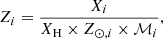 (1)
(1)
where XH is the hydrogen mass fraction of the gas particle.
To serve our showcase study, we investigated various lines of sight at each redshift according to the distribution of key physical quantities, such as temperature, density, and abundance. We qualitatively selected the two projected images presenting the most disturbed and structure-rich distributions (referred to as “irregular”), and the most regular and smoothed distributions (referred to as “regular”) of these quantities. These orientations are used to bracket the impact of projection effects.
2.2. Model of the ICM X-ray emission
To model the X-ray emission from our simulated cluster, we down-selected the SPH gas particles to those representative of the ICM in the gas temperature-density plane. We restricted the temperature range to 0.0808 < TkeV < 60. These boundaries are forced by the tabulated X-ray emission model used afterwards (i.e. vapec under XSPEC). We set an upper limit on the gas density of ne < 1 cm−3, to avoid overly dense regions in the simulations. These particles are not representative of the ICM properties, but would nonetheless bias our mock observations. These are likely particles recently affected by the supernovae and/or AGN feedback implementation. We removed about 100 particles out of a few million.
To model the X-ray emission of the cluster, we followed the procedure described in Cucchetti et al. (2018). For each selected gas particle, we assumed the collisionally ionised diffuse plasma model APEC (Smith et al. 2001) computed from the AtomDB v3.0.9. atomic database (Foster et al. 2012). We used its vapec implementation under XSPEC (Arnaud 1996) to account for the various chemical abundances traced in the Hydrangea simulations. The reference solar abundances are from Anders & Grevesse (1989) and the cross-sections are from Verner et al. (1996).
The redshift accounted for each particle reads as follows:
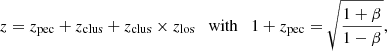 (2)
(2)
where zpec is linked to the peculiar velocity of the particles along the line of sight vlos within the clusters, and β = vlos/c, with c being the speed of light and zclus the cosmological redshift of the cluster.
The X-ray flux is directly proportional to the integral of the electron times proton density ne × nH over the particle volume V. Following the implementation in XSPEC the normalisation 𝒩 of the vapec model writes
![Mathematical equation: $$ \begin{aligned} \mathcal{N} = \frac{10^{-14}}{4 \pi [D_{\rm A}(1+z)]^2}\int _V n_{\rm e} n_{\rm H} \mathrm{d}V \quad \mathrm{(in\,cm^{-5})}, \end{aligned} $$](/articles/aa/full_html/2024/02/aa47612-23/aa47612-23-eq3.gif) (3)
(3)
with DA the angular diameter distance to the source (computed within the cosmological set-up of the Hydrangea simulations). We further assume ne = 1.2 × nH.
We fixed the value of the Galactic hydrogen column density to 0.03 × 1022 cm−2, a typical value for high galactic latitude. Its associated absorption of soft X-ray photons is modelled with a wabs model (Morrison & McCammon 1983).
From these hypotheses we computed the flux of photons at the Earth emitted by each particle. We used each particle’s X-ray spectrum in the range 0.2−12 keV as a density probability to draw the appropriate number of photons according to a given exposure time and collecting area. Stacked together over all cluster particles, we obtained a photon list at the Earth. The exposure time is systematically fixed to ten times that of the mock observation exposure in order to provide enough statistics for the instrumental simulations (see Sect. 3.) At this stage the collecting area is chosen to be 20 000 cm2, largely encompassing the area of the Athena mirrors over the whole energy band. This leads to an oversized list of photons providing proper statistics for the telescope and instrumental simulations, and avoids any duplication or undersampling biases.
3. Simulated X-IFU/Athena observations
3.1. The Athena telescope and X-IFU instrument
Athena is the next generation of X-ray telescopes from the European Space Agency (Barcons et al. 2017). It implements the science theme of the Hot and Energetic Universe (Nandra et al. 2013). With a focal length of 12 m it will embark a Wolter type I mirror initially expected to have a collecting area of 14 000 cm2 at 1 keV, and to provide a spatial resolution of 5 arcsec at full width at half maximum (FWHM). Two instruments will be on board, the Wide-Field Imager (WFI; Meidinger et al. 2017) and the X-ray Integral Field Unit (X-IFU; Barret et al. 2023).
In this study we focus on the capabilities of the X-IFU instrument, whose main initial high level performance requirements relevant for our study include a spectral resolution of 2.5 eV over the 0.2−7 keV band. This would represent a gain of a factor of ≈50 with respect to XMM-Newton. The effective area (constrained by the mirror collecting area) will be 10 000 cm2 at 1 keV, whilst the hexagonal field of view will have an equivalent diameter of 5 arcmin. We refer the reader to Barret et al. (2023) for a comprehensive description of the X-IFU instrument.
3.2. X-IFU mock observations
To simulate the observations with the X-IFU instrument, we followed the method described in Cucchetti et al. (2018) and summarised in the following. We made use of the SImulation of X-ray TElescopes software package (SIXTE; Wilms et al. 2014; Dauser et al. 2019). SIXTE ingests as input a SIMPUT (Schmid et al. 2013) file containing either emission spectra of individual sources or regions, or directly a list of photons at the telescope.
The SIXTE website3 distributes the baseline set-up for the X-IFU/Athena, as described in the previous section and detailed in Barret et al. (2023), formatted for the use of SIXTE. This includes resources and configurations such as focal plane geometry, point spread function (PSF), vignetting, instrumental background, cross-talk, the ancillary response file (ARF), and the redistribution matrix file (RMF), as provided by the X-IFU consortium4. We used this baseline set-up in this work.
We took into account the astrophysical emission from foreground and background emissions, and co-added them to our cluster of galaxies into a total photon list received at the Earth. We modelled the Galaxy halo and local bubble as diffuse emission according to the model proposed by McCammon et al. (2002), which is an absorbed (wabs*apec) and unabsorbed (apec) thermal plasma emission model, respectively. As per the required Athena spatial resolution, 80% of the sources constituting the extragalactic background are expected to be resolved (Moretti et al. 2003). This corresponds to a lower flux limit for individual simulated sources of ≈3 × 10⁻¹⁶ ergs s−1 cm−2 for a 100 ks exposure time (down-scaled to ≈10−16 ergs s−1 cm−2 for 1 Ms).
AGNs with fluxes below this limit were treated as a diffuse contribution, and modelled with an absorbed power-law spectrum parametrised as in McCammon et al. (2002). To avoid double-counting resolved AGNs, we set the normalisation of this model to 20% of its nominal value. The resolved cosmic X-ray background (CXB) was accounted for by adding the contribution of foreground and background AGNs according to the procedure described by Clerc et al. (2018). In short, AGNs were drawn from their luminosity function, N(L0.5 − 2 keV, z) (from Hasinger et al. 2005). Each source was assigned an emission spectrum from Gilli et al. (2007). They were then uniformly distributed over the simulated solid angle (thus neglecting any clustering effects). For both the Galactic and non-resolved CXB emission we used the model parameters provided by Lotti et al. (2014).
We fed the total (cluster of galaxies + astrophysical contamination) photon list to the xifupipeline method of SIXTE in order to generate a mock event list. All the above-mentioned instrumental effects and set-ups were accounted for, except for the cross-talk, which was irrelevant for our study. For each three redshifts and two line-of-sight orientations that we selected for our Hydrangea cluster (see Sect. 2.1 and Table 1), we generated two mock observations of one single pointing with 100 and 250 ks. For the cluster at z = 2, we also ran a third deep exposure of 1 Ms.
3.3. Processing of the mock data
For the purpose of our study, in our analysis we assumed spherical symmetry for the cluster, and we focused on a radial analysis.
3.3.1. Point source masking
We first proceeded by generating a raw count map, as shown in Fig. 1 for z = 2 and regular projection. As in Cucchetti et al. (2018), we flagged the loci of the simulated AGNs with fluxes above the limit defined in Sect. 3.2: ≈3 × 10⁻¹⁶ (≈10−16) ergs s−1 cm−2 for an exposure time of 100 ks (1 Ms). They were masked by excluding all the pixels with number counts 2σ above the mean count number of the pixels neighbouring their positions. This ensured that the ICM emission is accounted for. This procedure led to an effective flux threshold asymptotically reaching the value of ≈3 × 10⁻¹⁶ (10−16) ergs s−1 cm−2 with decreasing ICM emission. We performed a visual check and manually masked any remaining obvious point sources or overdense count regions that could arise from the Hydrangea simulation itself.
 |
Fig. 1. X-IFU map of a 100 ks raw number count for our Hydrangea cluster of galaxies at z = 2 and for “regular” projection. The image includes astrophysical and instrumental backgrounds. The green circles give the loci of the point sources to be excised. |
3.3.2. Surface brightness profile
We derived the surface brightness (SXB) profile from the raw count image masked from the point sources in order to account for the geometry of the X-IFU detector. We thus avoided artificially oversampling the intrinsic spatial resolution of the instrument (i.e. the convolution of the mirror PSF and the pixel size). The focal plane pixels were attributed to the radial annuli that encompass the position of their centre. Hence, the pattern of pixels populating the various radial annuli slowly tends to actual geometrical annuli over the detector array with increasing radius. However, the inner annuli significantly depart from such a regular shape. For instance, the central annulus contains a single pixel, whilst the second annulus contains the four nearest adjacent pixels to the central one in a cross pattern. This specific pattern is properly accounted for in the fit of the SXB profile (see Sect. 4).
In our mock observation, the position of the cluster projected centre, as defined in the Hydrangea simulations, coincides with the instrument optical axis. In other words, the cluster centre is positioned at the centre of the instrument detector array.
The SXB profile is extracted in the 0.4−1 keV band, where the bremsstrahlung emission of the ICM is still relatively flat, as a function of energy even at z = 2, and hence minimising its dependence on the gas temperature. The derived SXB profile for z = 2 and regular projection is presented in Sect. 5.
3.3.3. Spectral analysis
To recover the radial distribution of the gas temperature and chemical abundances, we binned our mock event list into six concentric annuli. As for the SXB profile, the centre was chosen to match the position of the projected centre of the simulated cluster.
The six annuli were defined to gather at least 10 000 counts in order to populate the spectral channels of the X-IFU. The spectra were extracted using the makespec function of SIXTE and binned according to the optimal method by Kaastra & Bleeker (2016). A specific ancillary response was computed per annulus accounting for the mirror vignetting weighted for each contributing pixel by its number counts.
The local background spectrum was extracted from the area of the field of view beyond R500. It was fitted with the model described in Sect. 3, that is apec+wabs*(apec+powerlaw). All parameters except for the three normalisations were fixed.
This best-fit background model was then rescaled to the area of each annulus (i.e. the pixel solid angle times the number of pixels belonging to the annulus) and fixed as such for the fit of the ICM model.
We fitted the spectra of the galaxy cluster with a wabs*vapec model under XSPEC with Cash statistics (Cash 1979), with the gas temperature, the normalisation and the Fe, Si, and Mg abundances as free parameters. We limited our investigation of the chemical abundances to these three elements as they present the most prominent lines with a reasonable probability to be detected out to a redshift of z = 2. All other abundances were fixed to the average value of the projected emission-measure weighted abundances from the Hydrangea halo particles over a given annulus. The reconstructed temperature and abundances radial distribution are shown in Sect. 5.
4. Forward-modelling and MCMC analysis
We chose a forward-modelling approach to fit the SXB, temperature, and abundance profiles in order to reconstruct the 3D radial distribution of the thermodynamical and chemical properties of the simulated cluster of galaxies. We recall that we assume spherical symmetry for our simulated clusters.
4.1. The forward-modelling procedure
We considered the gas density and pressure as two independent physical quantities in our model. We modelled the density distribution with a simplified Vikhlinin functional (Vikhlinin et al. 2006)
![Mathematical equation: $$ \begin{aligned} n_{\rm e}^2(x) = \frac{n_0^2}{(x/r_{\rm s})^{\alpha _1}[1+(x/r_{\rm s})^2]^{3\beta _1 - \alpha _1/2}}, \end{aligned} $$](/articles/aa/full_html/2024/02/aa47612-23/aa47612-23-eq4.gif) (4)
(4)
where x = r/R500, n0 is the central density, α1 and β1 are the inner and outer slopes, respectively, and rs is the scale radius.
The pressure radial distribution is described by a gNFW profile (Nagai et al. 2007)
![Mathematical equation: $$ \begin{aligned} P(x) = \frac{P_0}{(c_{500}\,x)^{\gamma }[1+(c_{500}\,x)^{\alpha _2}]^{(\beta _2-\gamma )/\alpha _2}}, \end{aligned} $$](/articles/aa/full_html/2024/02/aa47612-23/aa47612-23-eq5.gif) (5)
(5)
where P0 is the central pressure, c500 is the concentration at a radius of R500, and α2 and β2 are the intermediate and outer slopes, respectively. We do not have enough leverage with our observational constraints to fit γ, the inner slope. We thus leave it as a free parameter with a Gaussian prior with mean 0.43 and standard deviation of 0.1, the values derived from the XCOP sample (Ghirardini et al. 2019).
The temperature distribution is simply derived from the gas density and pressure assuming the ICM to be a perfect gas with P = ne × kBT (kB being the Boltzmann constant). The entropy is reconstructed assuming the conventionally adopted relation in X-ray astronomy, as introduced by Voit (2005):  .
.
For the radial distributions of chemical elements, we adopted a simple power-law model
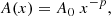 (6)
(6)
where A0 is specific to each element. However, we assumed the same slope p for all elements, considering it a fair assumption according to Mernier et al. (2017). The remaining 14 free parameters are listed in Table 2 together with their initial values and priors adopted in our Markov chain Monte Carlo (MCMC) fit.
Cluster model parameters.
We account for the parameter dispersion in each spherical shell by randomly drawing 5000 particles in the shell and adopting their values in density and pressure around the shell fiducial value. Our aim is to compare our results with volume-weighted distributions of the thermodynamic quantities (Sect. 5), so as to minimise the impact of high-density, small-volume particles; therefore, we weight the random draws by the volume of each particle. In doing so, we follow the dispersion of thermodynamic quantities predicted by the Hydrangea simulations about their fiducial profile. Figure 2 illustrates this process and shows how translating the cloud of particles in the log ne − log T plane provides a new distribution of densities and temperatures dispersed around a newly requested median value. These distributions are clipped at zero and at the maximum values allowed in our set-up (1 cm−3 and 15 keV). This process leads to 5000 spherically symmetric models, each contributing in equal proportion to the final model. Taken individually, they do not serve as realistic descriptions of the cluster; they serve as intermediate models, enabling propagation of the scatter in thermodynamic profiles.
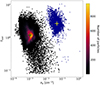 |
Fig. 2. Dispersion of thermodynamic quantities (electronic density ne in units of cm−3, and temperature T in units of keV) in one radial shell with 300 kpc < r < 310 kpc of the z = 2 cluster. The left cloud is a density map of extracted particles from the Hydrangea-simulated cluster. The green cross on the left indicates the position of the median density and temperature. The cloud of 5000 blue points on the right illustrates our random generation of a new model, when requesting a new set of median values (as shown by the yellow cross on the right). In this process, the shape of the dispersion in the log − log plane is essentially maintained fixed and translated. |
We compute the X-ray emission of the toy model cluster by averaging the emission of the 5000 models together. We apply an Abel transform, using the PyAbel5 Python package with the Hansenlaw transform method (Hansen & Law 1985) to each of the 5000 models, and average the resulting surface brightness profiles. Assuming circular symmetry, the profile is distributed into a 2D grid generously oversampling the X-IFU pixel size. Emission-measure-weighted temperature and abundance profiles are constructed similarly. We finally convolve these parameter grids with the PSF kernel and reshape the grids to the pixelisation and geometry of the X-IFU focal plane. We reproduce the source and pixel masking applied to the mock data. With this process we ensure a faithful reproduction of the input image characteristics (see Sect. 3.3).
4.2. The MCMC fit
We simultaneously fitted our SXB, temperature, and abundances profiles using a Bayesian MCMC approach. The modelling procedure described above (including the assessment and propagation of the parameter dispersion in shell) was reproduced at each step of the MCMC.
We formulated the associated likelihood as follows:
 (7)
(7)
Here yi, pj, σi, pj, and Mi are the mock data, associated mock error, and model for profile pj, respectively. The parameter pj denotes the set of the SXB, temperature, and Mn, Si, Fe abundance profiles. Such a likelihood implicitly assumes normal-distributed uncertainties. In the case of asymmetric uncertainties in the observable, we take σi, pj as the arithmetic mean of the upper and lower bounds of the 68% confidence level. Our MCMC sampling of the parameter space made use of the Python-based code emcee (Foreman-Mackey et al. 2019).
4.3. Validation
Before proceeding to the analysis of mock Hydrangea data, we first validate our fitting procedure using a simpler, spherically symmetric model. Its physical quantities (density, pressure, element abundances) are drawn following parametric profiles (Eqs. (4)–(6)). The numerical values are chosen so as to approximately reproduce the radial behaviour of the z = 2 cluster that we picked in the Hydrangea simulations (Table 1). In contrast with the Hydrangea cluster though, we impose each of these quantities, taking a single value within a spherical shell at radius r. This idealised model is transformed into a mock 100 ks X-IFU observation (as described in Sect. 3); this step includes the extraction of temperature and surface brightness profiles. We then fit the X-IFU mock observations with the exact same cluster model used to fit the actual simulation, letting 14 parameters freely evolve, namely n0, α1, β1, rs, P0, α2, β2, γ, c500, A0, i (i being one of Fe, Si, and Mg), p, and finally a uniform background level in the 0.4−1 keV imaging band. The priors and initial values for the 14 parameters are listed in Table 2.
Figure A.1 shows the results of our validation test. We find overall good agreement between the input model and the inferred properties. The 3D density and pressure profiles roughly agree with the input profiles within the 68% confidence intervals, at least across the radial range of applicability of our procedure (i.e. at radial distances located between the PSF size, r ≈ 0.1 R500, and the outermost radius, R500). Nevertheless, significant deviations appear, especially when considering the 2D temperature profiles and the comparison between the purple and black lines in the top right panel of Fig. A.1. Despite the simplicity of the input model, projection effects along the line of sight induce temperature and abundance mixing, which limit the ability of a single APEC model to account for the observed spectrum. This effect leads to underestimated uncertainties issued by the XSPEC fit (green error bars). In addition to this issue comes our as-yet-unverified assumption that weighting the 3D temperature by the emission-measure provides a fair representation of the 2D temperature profile. We checked that such deviations are not solely of statistical origin by increasing the exposure time of the mock observation to 1 Ms and finding similar offsets in the projected temperature profile (Fig. A.2). However, repeating the experiment with a toy model cluster placed at z = 1 provides better agreement in the recovered profiles (Fig. A.3). The larger apparent R500 compared to the z = 2 system enables a finer 2D binning of the temperature profiles to be defined (ultimately limited by the X-IFU pixel and/or PSF size), and hence mitigating the line-of-sight mixing effects.
In summary, our validation tests demonstrate the ability of our procedure to recover input profiles. However, we highlighted a limitation due to line-of-sight mixing of temperature (and abundances), attributed to both the finite X-IFU angular resolution relative to the z = 2 cluster angular span, and to the slight inadequacy of the spectral fitting model. These deviations propagate into the inference of the 3D thermodynamic profiles and limit our ability to recover their exact distributions. These limitations are in fact inherent to any observation of multi-phase diffuse gas, irrespective of the instrument in use.
5. Results
We now present the results obtained by fitting the z = 2 galaxy cluster extracted from the Hydrangea simulations (Sect. 2) and folded through the X-IFU instrumental response assuming a 100 ks exposure time. As we did for our validation model (see Sect. 4.3), we fit mock data with a spherically symmetric model with 14 free parameters. They are listed in Table 2. They are used in Eqs. (4)–(6) and govern the median 3D model for ne(r), P(r), and A(r). The 13th parameter is an additional background level in the 0.4 − 1 keV imaging band. Accounting for the intrinsic dispersion of these quantities around their median values requires prior knowledge of its radial behaviour (or a parametrised model thereof). We simply assumed that the dispersion in the (log ne, log T) plane follows that of the Hydrangea cluster in each radial shell (see Fig. 2 and Sect. 4.1). This assumption avoids introducing additional model parameters, although we expect that using the exact dispersion for the forward-model may put our results on the optimistic side. For computational reasons, we do not assume any dispersion of the abundance within a spherical shell in our forward-model.
Figures 3–5 illustrate the outcome of the forward-modelling procedure. In each figure the uncertainty on the 14 free model parameters is propagated and provides the envelope indicated with the red dashed lines. In contrast to the validation model (e.g. Fig. A.1), our visualisation now incorporates the effect of the intrinsic dispersion in the thermodynamic quantities, which is a key ingredient in our model. In each figure (except for the chemical abundances) this intrinsic dispersion is added in quadrature to the parameter uncertainties in order to provide the red shaded envelope.
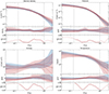 |
Fig. 3. Three-dimensional thermodynamic quantities (in blue) for the z = 2 galaxy cluster with regular projection in the Hydrangea sample, and their best-fit models inferred from an X-IFU 100 ks exposure (in red). Each panel representing one quantity is made up of three plots. The top curve displays the radial profiles; the blue shaded envelope represents the dispersion of the gas particles in the hydro-simulation. The red dashed lines indicates the effect of the variance of the 14 free model parameters; the shaded envelope also includes the radial dispersion encapsulated in our model. The middle plot represents the deviation of the profile relative to the input median profile. The bottom plot shows the results of a Kolmogorov–Smirnov (KS) test performed at each radius r/r500, related to the probability that the input and best-fit profiles do not originate from the same distribution (the lower the KS, the closer the agreement between the profiles). The vertical lines indicate the range of applicability of our modelling procedure. |
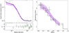 |
Fig. 4. Projected observables and their best-fit models for the z = 2 galaxy cluster with regular projection in the Hydrangea sample, as seen by X-IFU in a 100 ks exposure. Left: Surface brightness profile in the 0.4−1 keV band and its uncertainties (green points). The posterior mean (best-fit model) and its 68% confidence envelope are represented in purple. The bottom panel displays the deviation of the measurements relative to the best fit, normalised by the errors. Right: 2D temperature profile as measured by XSPEC in each annular bin (green points and errors). The emission-measure-weighted temperature TEM (known from the hydrodynamic simulation) is shown as a thick black line. In both panels the shaded purple envelope includes both the contribution of the intrinsic dispersion of physical quantities within the radial shells and the propagated variance of the 14 free model parameters (dashed lines). |
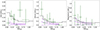 |
Fig. 5. Projected abundance profiles and their best-fit models for the z = 2 galaxy cluster with regular projection in the Hydrangea sample, as seen by X-IFU in a 100 ks exposure. Each panel corresponds to one chemical element of Fe, Si, and Mg. The measurement output by XSPEC is shown as green points (and errors). The emission-measure-weighted abundance profile (known as input) is displayed as a thick black line. The best-fit model is displayed in purple, and the dashed lines represent the error of the free model parameters. |
The profiles built from simulation particles also incorporate intrinsic dispersion. In each radial shell we computed the particle-volume weighted histogram of a given quantity (e.g. density). Figure 3 shows the associated 16th, 50th, and 84th percentiles as a plain blue line and a blue shaded envelope.
Focusing first on the recovery of physical thermodynamic quantities (electron density ne, pressure P, temperature T, and entropy K in Fig. 3) we find a qualitatively good agreement between the profiles recovered from the fit and the input profiles. The large amount of intrinsic dispersion within each spherical shell makes the comparison of the median profiles cumbersome since a unique density (respectively pressure, temperature, entropy) does not exist at a given radius, rather there is a distribution of densities (respectively P, T, K). In order to quantify the agreement between the input and the fitted profiles, we performed a two-sample Kolmogorov–Smirnov (KS) test in thin shells at each radius r, by comparing the distribution of density values ne (respectively P, T, K) of the Hydrangea simulations to the distribution of densities (respectively P, T, K) sampled by the MCMC. The KS statistic is related to the probability of rejecting the null hypothesis, given that the two distributions originate from the same (unknown) distribution. The lower the KS value, the more confident we are that the two profiles are in agreement with each other. We also computed the average value of the KS statistic over the radial range between the PSF size and R500, and we listed the values in Table 3 (in bold characters).
Kolmogorov–Smirnov test results.
Folding the MCMC parameter samples through our model provides the distribution of projected observables, namely the 0.4−1 keV surface brightness (Fig. 4, left) and the emission-measure-weighted temperature (Fig. 4, right). Most of the dispersion in surface brightness posterior samples originates from the intrinsic dispersion of thermodynamic quantities (mostly ne), while statistical uncertainties on the profiles arising from the MCMC have little impact on the global error budget. The deviation of the reconstructed surface brightness profile, relative to the statistical error, is at most 1.4. The variance in the posterior projected temperature is roughly equally shared between intrinsic dispersion and parameter uncertainties. Similarly to the validation case (Sect. 4.3 and Fig. A.1), some deviations appear between the best-fit and input models, although they are contained within the 1σ envelope. A noticeable outlier is the XSPEC-fitted temperature in the fourth radial bin at R ≃ 0.45 R500. Part of this bias is due to mixing effects along the line of sight and to a spectral model that is unable to account for such mixed components. The bias is also caused by a relatively faint CXB point source located within the brighter cluster region. It is therefore absent from the set of excised points sources (circles in Fig. 1). This unmasked point source brings an excess of high-energy photons in the fourth radial bin spectrum, that is sufficient to bias high the XSPEC measurement. The deviation of the reconstructed temperature, relative to the statistical error, is at most 2.9 and at most 1 if we remove the failed measurement in the fourth annulus.
The inference of chemical abundance profiles is depicted in Fig. 5. None of the profiles is correctly recovered; in other words, the 68% posterior confidence level (dashed purple envelope) does not reproduce well the EM-weighted abundance profile (black thick line) known as input from the hydrodynamical simulation. It is worth noting how XSPEC-fitted abundances scatter widely around the expected values, denoting both a lack of statistics and the inadequacy of the spectral model due to the mixing of components. The apparent underestimation of posterior abundance profiles originates from the low signal-to-noise ratios and to an improper use of a Gaussian likelihood (Eq. (7)) for strictly positive abundance values. We verified that increasing the X-IFU exposure to 1 Ms provides a decent recovery of the iron (Fe) and silicon (Si) profiles, while magnesium (Mg) is still affected by poor statistics (see Sect. 6 and Fig. B.3). Such a result is not surprising, due to the faintness of the cluster emission and to the large dispersion of abundances along a single line of sight in the Hydrangea simulations (which is spatially correlated with density and temperature), and thus to the inability of our model to adequately capture the 3D structure of the element abundances in such a complex object. This issue is exacerbated by our choice of a crude spatial binning, mostly targeted towards temperature extraction (see e.g. Cucchetti et al. 2018, which presents an alternative binning scheme tailored to abundance measurements).
6. Discussion
6.1. Inferring the properties of a z = 2 cluster of galaxies
Our analysis demonstrates the capability to infer the (volume-weighted) thermodynamic properties of a realistic cluster of galaxies located at z = 2, using a moderate exposure budget of 100 ks with X-IFU on board Athena. Despite the compact faint appearance of this low-mass object at such large cosmological distances (Fig. 1), the effective radial range accessible to X-IFU spans almost one decade between ≈0.1 − 1 R500. This enables recovery of the shape, amplitude, and characteristic slopes of the profiles. The finite instrumental angular resolution prevents accessing smaller scales and resolving core properties.
The density and pressure profiles are the quantities best reconstructed in comparison to the input data, with deviations of the median profile reaching 20% at most. Temperature and entropy display more noticeable deviations, up to 50% when considering the median profiles. The explanation for this difference relates to the fact that temperature and entropy are deduced from the other two. Therefore, their uncertainties propagate the errors of both density and pressure profiles. Moreover, this difference is also related to our primary observables used for inference. Since surface brightness profiles are measured with much less uncertainty than projected temperature (see e.g. Fig. 4), quantities heavily dependent on temperature (temperature itself and entropy) are much more strongly affected by measurement systematics than density and pressure.
Our z = 2 study highlights a key point: the ICM is not spherically symmetric, nor is it homogeneous within a given radial shell, making a mere comparison of median profiles insufficient for us to grasp the complete reality of the scientific problem. For this reason we also compared the distributions of the thermodynamic quantities at fixed radius. Our radially dependent KS statistic test indicates again that the recovered density and pressure relate well to the Hydrangea simulations, with the KS statistics spanning values between 0 and 0.2. Entropy and pressure may display KS values up to 0.4 − 0.5, notably in the centre where PSF blurring is significant. The KS indicator is also elevated at radial locations affected by a faulty XSPEC measurement (Fig. 4, right, at R ≃ R500/2 in this example). Such a systematic error is not solely due to poor statistics, nor to inhomogeneity in the cluster gas distribution. We have shown that this error acts as a floor uncertainty, inherent to our analysis set-up. First, the inability of a single APEC model to account for a multi-temperature plasma projected along the line of sight induces discrepancies that are not well captured by the XSPEC error bars. The development of multi-temperature spectral models with arbitrary distributions of emission measure (e.g. generalising the class of gadem models) would certainly benefit high-resolution spectroscopy of diffuse astrophysical plasmas. Moreover, the identification of point sources contaminating the spectral measurements and buried in the cluster emission should also enhance the quality of spectral fits. Second, we worked under the assumption that emission-measure weighting fairly represents the measured X-IFU spectroscopic temperature. Previous studies focusing on XMM-Newton and Chandra instead proposed “spectroscopic-like” weightings in order to alleviate this concern (e.g. Mazzotta et al. 2004; Vikhlinin 2006). We verified that spectroscopic-like temperature profiles are even more discrepant with measurements than emission-measure weighted profiles. Such a work is waiting to be realised in the case of high-resolution instruments like the X-IFU. More generally, our study calls for further development of new analysis tools dedicated to the analysis of hyperspectral imaging of extended structures (e.g. Picquenot et al. 2019), with an ability to handle the regime of a low number of counts.
6.2. Impact of deeper observations and of targeting a cluster at a more mature evolutionary stage
So far, our results and discussion have focused on a single galaxy cluster extracted from the z = 2 simulation snapshot. Observing this cluster of galaxies at later times (i.e. at lower redshifts, z = 1 and 1.5) brings a supplementary amount of information to our study. At later epochs this cluster is more massive, more extended, hotter, and intrinsically more luminous (Table 1). This leads to an increase in the signal-to-noise ratios in observables, both the surface brightness and spectra. Being closer to the observer, the surface brightness is also less faint, and hence another increase in signal-to-noise ratios. We note however that the angular diameter distance hardly changes over this range of redshifts, by a few percent at most. Therefore, little gain is expected from angular resolution effects. We replicated the analysis shown previously for all 14 configurations displayed in Table 3. In each case we inferred the four thermodynamic profiles and the three abundance profiles, accounting for the intrinsic dispersion within a radial shell. We inspected the results in light of deviations from the known input profiles. Although the fidelity of the profile reconstruction has a strong radial dependence, we summarise here our results with a single quantity, namely the average of the KS tests performed over the whole range of radii comprised between the PSF size and R500 (Table 3).
In general, moving the cluster closer to the observer provides an enhancement in the accuracy of the reconstructed thermodynamic profiles and abundance profiles, as does increasing the exposure time. This is especially visible for the density profiles, whose inference relies primarily on surface brightness profiles. However, we found significant outliers to this overall trend, due to the systematic effects already discussed in Sect. 5 and Appendix B. A single faulty temperature measurement in one radial bin (e.g. due to mixing components by projection along the line of sight) has a negative impact on all reconstructed quantities. Surprisingly, such situations may occur even at low redshifts and/or for large exposure times. One such example is the z = 1, irregular configuration, which seems better characterised at 100 ks than at 250 ks. A second example is the z = 2, 250 ks, regular configuration, which comprises a catastrophic temperature measurement, hence shifting the reconstructed profiles considerably away from the true one. We also find that observing the cluster in an orientation that minimises the projection of gas phases along the line of sight and maximises the asymmetries in the plane of the image (i.e. the irregular case) often slightly improves the reconstruction of profiles, consistent with our expectations.
6.3. Perspectives
This work presents the results of one single test case. This object may display peculiarities that are not representative of the entire population of groups and clusters. A complete assessment of the scientific feasibility related to thermodynamic profile inference with X-IFU would involve a larger sample of objects. On the one hand, singularities associated with a single test case would average out; on the other hand, this would more closely match the approach that observers take in studying intracluster and intragroup physics.
The study presented in this paper was conducted with the current public science requirements for the Athena missions and the X-IFU instruments. The Athena mission is currently undergoing a complete reformulation of its science case and consequently of the specifications of its instruments. The outcomes of our study might be modulated by the outcome of this reformulation.
As pointed out in the Introduction, we limited our study to an investigation with the X-IFU instrument following the specifications from the Athena Mock Observing Plan. However, we note that a natural extension of the presented work would be to investigate distant groups of galaxies with deep pointed observations with the second Athena instrument, the Wide-Field Imager (WFI; Rau et al. 2017), and in combination with X-IFU observations. This would optimise the physical characterisation of these objects, at the expense of exposure time as the two instruments will not be observing simultaneously.
Accounting for the current Athena mock observing plan specifications and the ongoing reformulation process for the Athena mission, we will implement this dual combination in a forthcoming investigation. The upcoming XRISM mission will soon provide the community with unprecedented X-ray observations with high spectral resolution of nearby bright objects. More distant objects such as the first groups of galaxies will have to wait for the advent of observations by the next generation of X-ray integral field units, such as the X-IFU instrument on board the Athena mission or the Line Emission Mapper (LEM) mission concept (Kraft et al. 2022).
Version v4.3 issued on 8 September 2020 by the ESA Athena Science Study Team, the science objective regarding the evolution of thermodynamical properties of groups and clusters of galaxies from z > 0.5 and out to z ∼ 2 will be achieved with X-IFU observations. We therefore focused in this study on this specific instrument only.
We made use of the Hydrangea Python library: https://hydrangea.readthedocs.io/en/latest/index.html
Acknowledgments
The authors would like to thank Dominique Eckert for refereeing this paper and for providing insightful comments on the study. E.P., F.C. and N.C. acknowledge the support of CNRS/INSU and CNES. J.S. acknowledges the support of The Netherlands Organisation for Scientific Research (NWO) through research programme Athena 184.034.002. Y.M.B. gratefully acknowledges funding from the Netherlands Research Organisation (NWO) through Veni grant number 639.041.751, and financial support from the Swiss National Science Foundation (SNSF) under project 200021_213076.
References
- Anders, E., & Grevesse, N. 1989, Geochim. Cosmochim. Acta, 53, 197 [Google Scholar]
- Arnaud, K. A. 1996, in Astronomical Data Analysis Software and Systems V, eds. G. H. Jacoby, & J. Barnes, ASP Conf. Ser., 101, 17 [NASA ADS] [Google Scholar]
- Babyk, I. V., & McNamara, B. R. 2023, ApJ, 946, 54 [NASA ADS] [CrossRef] [Google Scholar]
- Bahé, Y. M., Barnes, D. J., Dalla Vecchia, C., et al. 2017, MNRAS, 470, 4186 [Google Scholar]
- Barcons, X., Barret, D., Decourchelle, A., et al. 2017, Astron. Nachr., 338, 153 [NASA ADS] [CrossRef] [Google Scholar]
- Barnes, D. J., Kay, S. T., Bahé, Y. M., et al. 2017, MNRAS, 471, 1088 [Google Scholar]
- Barret, D., Albouys, V., Herder, J.-W. D., et al. 2023, Exp. Astron., 55, 373 [NASA ADS] [CrossRef] [Google Scholar]
- Behroozi, P. S., Wechsler, R. H., & Conroy, C. 2013, ApJ, 770, 57 [NASA ADS] [CrossRef] [Google Scholar]
- Biffi, V., Planelles, S., Borgani, S., et al. 2017, MNRAS, 468, 531 [Google Scholar]
- Booth, C. M., & Schaye, J. 2009, MNRAS, 398, 53 [Google Scholar]
- Cash, W. 1979, ApJ, 228, 939 [Google Scholar]
- Clerc, N., Ramos-Ceja, M. E., Ridl, J., et al. 2018, A&A, 617, A92 [NASA ADS] [CrossRef] [EDP Sciences] [Google Scholar]
- Clerc, N., Cucchetti, E., Pointecouteau, E., & Peille, P. 2019, A&A, 629, A143 [NASA ADS] [CrossRef] [EDP Sciences] [Google Scholar]
- Crain, R. A., Schaye, J., Bower, R. G., et al. 2015, MNRAS, 450, 1937 [NASA ADS] [CrossRef] [Google Scholar]
- Cucchetti, E., Pointecouteau, E., Peille, P., et al. 2018, A&A, 620, A173 [NASA ADS] [CrossRef] [EDP Sciences] [Google Scholar]
- Cucchetti, E., Clerc, N., Pointecouteau, E., Peille, P., & Pajot, F. 2019, A&A, 629, A144 [NASA ADS] [CrossRef] [EDP Sciences] [Google Scholar]
- Dalla Vecchia, C., & Schaye, J. 2012, MNRAS, 426, 140 [NASA ADS] [CrossRef] [Google Scholar]
- Dauser, T., Falkner, S., Lorenz, M., et al. 2019, A&A, 630, A66 [NASA ADS] [CrossRef] [EDP Sciences] [Google Scholar]
- Eckert, D., Gaspari, M., Gastaldello, F., Le Brun, A. M. C., & O’Sullivan, E. 2021, Universe, 7, 142 [NASA ADS] [CrossRef] [Google Scholar]
- Foreman-Mackey, D., Farr, W., Sinha, M., et al. 2019, J. Open Source Softw., 4, 1864 [NASA ADS] [CrossRef] [Google Scholar]
- Foster, A. R., Ji, L., Smith, R. K., & Brickhouse, N. S. 2012, ApJ, 756, 128 [Google Scholar]
- Ghirardini, V., Eckert, D., Ettori, S., et al. 2019, A&A, 621, A41 [NASA ADS] [CrossRef] [EDP Sciences] [Google Scholar]
- Gilli, R., Comastri, A., & Hasinger, G. 2007, A&A, 463, 79 [NASA ADS] [CrossRef] [EDP Sciences] [Google Scholar]
- Haardt, F., & Madau, P. 2001, in Clusters of Galaxies and the High Redshift Universe Observed in X-rays, eds. D. M. Neumann, & J. T. V. Tran, 64 [Google Scholar]
- Hansen, E. W., & Law, P.-L. 1985, J. Opt. Soc. Am. A, 2, 510 [NASA ADS] [CrossRef] [Google Scholar]
- Hasinger, G., Miyaji, T., & Schmidt, M. 2005, A&A, 441, 417 [NASA ADS] [CrossRef] [EDP Sciences] [Google Scholar]
- Kaastra, J. S., & Bleeker, J. A. M. 2016, A&A, 587, A151 [NASA ADS] [CrossRef] [EDP Sciences] [Google Scholar]
- Kraft, R., Markevitch, M., Kilbourne, C., et al. 2022, arXiv e-prints [arXiv:2211.09827] [Google Scholar]
- Kravtsov, A. V., & Borgani, S. 2012, ARA&A, 50, 353 [Google Scholar]
- Lambert, T. S., Kraan-Korteweg, R. C., Jarrett, T. H., & Macri, L. M. 2020, MNRAS, 497, 2954 [Google Scholar]
- Leauthaud, A., Tinker, J., Bundy, K., et al. 2012, ApJ, 744, 159 [Google Scholar]
- Lotti, S., Cea, D., Macculi, C., et al. 2014, A&A, 569, A54 [NASA ADS] [CrossRef] [EDP Sciences] [Google Scholar]
- Lovisari, L., & Maughan, B. J. 2022, in Handbook of X-ray and Gamma-ray Astrophysics, eds. C. Bambi, & A. Santangelo, 65 [Google Scholar]
- Lovisari, L., Reiprich, T. H., & Schellenberger, G. 2015, A&A, 573, A118 [NASA ADS] [CrossRef] [EDP Sciences] [Google Scholar]
- Lovisari, L., Ettori, S., Gaspari, M., & Giles, P. A. 2021, Universe, 7, 139 [NASA ADS] [CrossRef] [Google Scholar]
- Mazzotta, P., Rasia, E., Moscardini, L., & Tormen, G. 2004, MNRAS, 354, 10 [NASA ADS] [CrossRef] [Google Scholar]
- McCammon, D., Almy, R., Apodaca, E., et al. 2002, ApJ, 576, 188 [NASA ADS] [CrossRef] [Google Scholar]
- McNamara, B. R., & Nulsen, P. E. J. 2007, ARA&A, 45, 117 [NASA ADS] [CrossRef] [Google Scholar]
- Meidinger, N., Barbera, M., Emberger, V., et al. 2017, in Proc. SPIE, ed. O. H. Siegmund, 10397, 103970V [NASA ADS] [Google Scholar]
- Mernier, F., de Plaa, J., Kaastra, J. S., et al. 2017, A&A, 603, A80 [NASA ADS] [CrossRef] [EDP Sciences] [Google Scholar]
- Mernier, F., Biffi, V., Yamaguchi, H., et al. 2018, Space Sci. Rev., 214, 129 [Google Scholar]
- Mernier, F., Cucchetti, E., Tornatore, L., et al. 2020, A&A, 642, A90 [NASA ADS] [CrossRef] [EDP Sciences] [Google Scholar]
- Moretti, A., Campana, S., Lazzati, D., & Tagliaferri, G. 2003, ApJ, 588, 696 [NASA ADS] [CrossRef] [Google Scholar]
- Morrison, R., & McCammon, D. 1983, ApJ, 270, 119 [Google Scholar]
- Nagai, D., Kravtsov, A. V., & Vikhlinin, A. 2007, ApJ, 668, 1 [Google Scholar]
- Nandra, K., Barret, D., Barcons, X., et al. 2013, arXiv e-prints [arXiv:1306.2307] [Google Scholar]
- Oppenheimer, B. D., Babul, A., Bahé, Y., Butsky, I. S., & McCarthy, I. G. 2021, Universe, 7, 209 [NASA ADS] [CrossRef] [Google Scholar]
- Picquenot, A., Acero, F., Bobin, J., et al. 2019, A&A, 627, A139 [EDP Sciences] [Google Scholar]
- Planck Collaboration XVI. 2014, A&A, 571, A16 [NASA ADS] [CrossRef] [EDP Sciences] [Google Scholar]
- Ponman, T. J., Sanderson, A. J. R., & Finoguenov, A. 2003, MNRAS, 343, 331 [NASA ADS] [CrossRef] [Google Scholar]
- Rau, A., Nandra, K., Meidinger, N., & Plattner, M. 2017, in The X-ray Universe 2017, eds. J. U. Ness, & S. Migliari, 24 [Google Scholar]
- Roncarelli, M., Gaspari, M., Ettori, S., et al. 2018, A&A, 618, A39 [NASA ADS] [CrossRef] [EDP Sciences] [Google Scholar]
- Sanderson, A. J. R., O’Sullivan, E., Ponman, T. J., et al. 2013, MNRAS, 429, 3288 [NASA ADS] [CrossRef] [Google Scholar]
- Schaller, M., Dalla Vecchia, C., Schaye, J., et al. 2015, MNRAS, 454, 2277 [NASA ADS] [CrossRef] [Google Scholar]
- Schaye, J., & Dalla Vecchia, C. 2008, MNRAS, 383, 1210 [Google Scholar]
- Schaye, J., Dalla Vecchia, C., Booth, C. M., et al. 2010, MNRAS, 402, 1536 [Google Scholar]
- Schaye, J., Crain, R. A., Bower, R. G., et al. 2015, MNRAS, 446, 521 [Google Scholar]
- Schaye, J., Kugel, R., Schaller, M., et al. 2023, MNRAS, 526, 4978 [NASA ADS] [CrossRef] [Google Scholar]
- Schmid, C., Smith, R. K., & Wilms, J. 2013, SIMPUT– A File Format for Simulation Input (Cambridge: HEASARC) [Google Scholar]
- Smith, R. K., Brickhouse, N. S., Liedahl, D. A., & Raymond, J. C. 2001, ApJ, 556, L91 [Google Scholar]
- Springel, V. 2005, MNRAS, 364, 1105 [Google Scholar]
- Stott, J. P., Hickox, R. C., Edge, A. C., et al. 2012, MNRAS, 422, 2213 [NASA ADS] [CrossRef] [Google Scholar]
- Sun, M., Sehgal, N., Voit, G. M., et al. 2011, ApJ, 727, L49 [NASA ADS] [CrossRef] [Google Scholar]
- Tinker, J., Kravtsov, A. V., Klypin, A., et al. 2008, ApJ, 688, 709 [Google Scholar]
- Verner, D. A., Ferland, G. J., Korista, K. T., & Yakovlev, D. G. 1996, ApJ, 465, 487 [Google Scholar]
- Vikhlinin, A. 2006, ApJ, 640, 710 [NASA ADS] [CrossRef] [Google Scholar]
- Vikhlinin, A., Kravtsov, A., Forman, W., et al. 2006, ApJ, 640, 691 [Google Scholar]
- Vogelsberger, M., Genel, S., Springel, V., et al. 2014, MNRAS, 444, 1518 [Google Scholar]
- Voit, G. M. 2005, Rev. Mod. Phys., 77, 207 [Google Scholar]
- Walsh, S., McBreen, S., Martin-Carrillo, A., et al. 2020, A&A, 642, A24 [NASA ADS] [CrossRef] [EDP Sciences] [Google Scholar]
- Werner, S. V., Cypriano, E. S., Gonzalez, A. H., et al. 2023, MNRAS, 519, 2630 [Google Scholar]
- Wiersma, R. P. C., Schaye, J., & Smith, B. D. 2009a, MNRAS, 393, 99 [NASA ADS] [CrossRef] [Google Scholar]
- Wiersma, R. P. C., Schaye, J., Theuns, T., Dalla Vecchia, C., & Tornatore, L. 2009b, MNRAS, 399, 574 [NASA ADS] [CrossRef] [Google Scholar]
- Wijers, N. A., & Schaye, J. 2022, MNRAS, 514, 5214 [NASA ADS] [CrossRef] [Google Scholar]
- Wijers, N. A., Schaye, J., & Oppenheimer, B. D. 2020, MNRAS, 498, 574 [NASA ADS] [CrossRef] [Google Scholar]
- Wilms, J., Brand, T., Barret, D., et al. 2014, in Space Telescopes and Instrumentation 2014: Ultraviolet to Gamma Ray, eds. T. Takahashi, J. W. A. den Herder, & M. Bautz, SPIE Conf. Ser., 9144, 91445X [Google Scholar]
Appendix A: Results of our validation tests
We show here the results of our validation tests on a simpler, spherically symmetric model. These tests are described in Sect. 4.3. Figures A.1 and A.2 differ only by the net exposure time of the mock X-IFU observation, respectively 100 ks and 1 Ms.
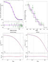 |
Fig. A.1. Validation of the forward-modelling procedure. The input model is a spherically symmetric cluster at z = 2, transformed into a 100 ks mock X-IFU observation. Top left: Surface brightness profile from the mock 0.4–1 keV image (green points and errors). The posterior mean (best-fit model) and the 68% confidence range appear as a purple solid line and dashed envelope. The sub-panel represents the difference between measurements and the best-fit model, normalised by the uncertainties. Top right: 2D temperature profile measured from X-IFU mock events using XSPEC (green points and errors). The emission-measure-weighted temperature TEM known as input is displayed as a thick black line. The posterior mean (best-fit model) and the 68% envelope are shown in purple (solid and dashed lines, respectively). Bottom panels: Inferred electron density (left) and pressure (right) profiles are represented with the red line and dashed envelope (68% confidence level). The input profiles are in blue, and follow Eqs. 4 and 5, respectively. The two sub-panels represent the deviation of the best-fit models relative to the true input profiles. The range of fidelity of our fit is located between the PSF size (indicated with the leftmost vertical dashed line) and R500 (rightmost line). |
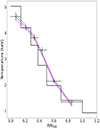 |
Fig. A.2. Similar to Fig. A.1 (top right), but for a 1 Ms X-IFU exposure. This represents the outcome of our validation test in a regime of high photon statistics, and it exacerbates the issue due to mixing gas temperatures along the line of sight of this z = 2 idealised cluster model. |
Figure A.1 is related to our baseline validation at 100 ks X-IFU exposure for a z = 2 cluster. Figure A.2 refers to the same cluster, but for a 1 Ms exposure, and we highlight the residual uncertainties not solved by increasing the photon statistics. Finally, Fig. A.3 is for a 100 ks exposure of a much nearer z = 1 prototypical cluster, whose physical and angular sizes (R500 in kpc and in arcminutes) are about twice those of the z = 2 cluster. In this case the cluster emission is better resolved by the X-IFU instrument, and mixing effects in the spectral fits are less of a concern.
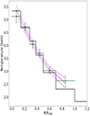 |
Fig. A.3. Similar to Fig. A.1 (top right), but for a validation cluster placed at z = 1 (still at a 100 ks X-IFU exposure). Because each resolution element in the X-IFU image ‘sees’ a smaller region (in units of R500), the mixing effects appear less prominent than in the z = 2 case. The reconstructed and XSPEC-fitted temperature profiles are therefore closer to the input EM-weighted profile. |
Appendix B: Results for a 1 Ms exposure on the z = 2 cluster
In order to gauge the ultimate capabilities of X-IFU in precisely determining the gas content of the z = 2 cluster, we reproduced the experiment of Sect. 5 using a 1 Ms exposure instead of 100 ks. We illustrate two salient results obtained by increasing the exposure time by a factor of 10. On the one hand, XSPEC temperature measurements show reduced error bars due to higher signal-to-noise ratios in the fitted spectra (Figs. B.1); however, the disagreement with the EM-weighted input model still persists. As hinted in our validation experiment (Sect. 4.3), this may be attributed to projection effects mixing components in the resulting observables, which are not solved solely by increasing the statistics. We demonstrate this by running our analysis on the same cluster, although observed from an alternative orientation selected so that it minimises the projection effects along the line of sight. Figure B.2 shows the result obtained for that configuration; the green, black, and purple curves clearly appear closer to each other, despite some residual deviations due to remaining mixing effects.
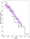 |
Fig. B.1. Similar to Fig. 4 (right), but for a 1 Ms mock X-IFU exposure. Despite the tenfold increase in photon statistics, the complex structure of the z = 2 Hydrangea cluster prevents us from achieving a perfect reconstruction of the projected temperature profile, mainly because of faulty XSPEC single-temperature fits (green points and errors). |
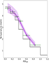 |
Fig. B.2. Similar to Fig. B.1, but the cluster is observed along a line of sight that minimises projection effects. Mixing issues are mitigated by selecting this cluster orientation, enabling a more faithful reconstruction of the cluster profiles. |
On the other hand, the reconstruction of abundance profiles at a 1 Ms exposure (Fig. B.3) appears more satisfactory when compared to the 100 ks case (Fig. 5), with both iron (Fe) and silicon (Si) profiles well recovered by the forward-model. Only magnesium still presents diverging results despite the tenfold increase in photon statistics.
All Tables
All Figures
|
Fig. 1. X-IFU map of a 100 ks raw number count for our Hydrangea cluster of galaxies at z = 2 and for “regular” projection. The image includes astrophysical and instrumental backgrounds. The green circles give the loci of the point sources to be excised. |
| In the text | |
|
Fig. 2. Dispersion of thermodynamic quantities (electronic density ne in units of cm−3, and temperature T in units of keV) in one radial shell with 300 kpc < r < 310 kpc of the z = 2 cluster. The left cloud is a density map of extracted particles from the Hydrangea-simulated cluster. The green cross on the left indicates the position of the median density and temperature. The cloud of 5000 blue points on the right illustrates our random generation of a new model, when requesting a new set of median values (as shown by the yellow cross on the right). In this process, the shape of the dispersion in the log − log plane is essentially maintained fixed and translated. |
| In the text | |
|
Fig. 3. Three-dimensional thermodynamic quantities (in blue) for the z = 2 galaxy cluster with regular projection in the Hydrangea sample, and their best-fit models inferred from an X-IFU 100 ks exposure (in red). Each panel representing one quantity is made up of three plots. The top curve displays the radial profiles; the blue shaded envelope represents the dispersion of the gas particles in the hydro-simulation. The red dashed lines indicates the effect of the variance of the 14 free model parameters; the shaded envelope also includes the radial dispersion encapsulated in our model. The middle plot represents the deviation of the profile relative to the input median profile. The bottom plot shows the results of a Kolmogorov–Smirnov (KS) test performed at each radius r/r500, related to the probability that the input and best-fit profiles do not originate from the same distribution (the lower the KS, the closer the agreement between the profiles). The vertical lines indicate the range of applicability of our modelling procedure. |
| In the text | |
|
Fig. 4. Projected observables and their best-fit models for the z = 2 galaxy cluster with regular projection in the Hydrangea sample, as seen by X-IFU in a 100 ks exposure. Left: Surface brightness profile in the 0.4−1 keV band and its uncertainties (green points). The posterior mean (best-fit model) and its 68% confidence envelope are represented in purple. The bottom panel displays the deviation of the measurements relative to the best fit, normalised by the errors. Right: 2D temperature profile as measured by XSPEC in each annular bin (green points and errors). The emission-measure-weighted temperature TEM (known from the hydrodynamic simulation) is shown as a thick black line. In both panels the shaded purple envelope includes both the contribution of the intrinsic dispersion of physical quantities within the radial shells and the propagated variance of the 14 free model parameters (dashed lines). |
| In the text | |
|
Fig. 5. Projected abundance profiles and their best-fit models for the z = 2 galaxy cluster with regular projection in the Hydrangea sample, as seen by X-IFU in a 100 ks exposure. Each panel corresponds to one chemical element of Fe, Si, and Mg. The measurement output by XSPEC is shown as green points (and errors). The emission-measure-weighted abundance profile (known as input) is displayed as a thick black line. The best-fit model is displayed in purple, and the dashed lines represent the error of the free model parameters. |
| In the text | |
|
Fig. A.1. Validation of the forward-modelling procedure. The input model is a spherically symmetric cluster at z = 2, transformed into a 100 ks mock X-IFU observation. Top left: Surface brightness profile from the mock 0.4–1 keV image (green points and errors). The posterior mean (best-fit model) and the 68% confidence range appear as a purple solid line and dashed envelope. The sub-panel represents the difference between measurements and the best-fit model, normalised by the uncertainties. Top right: 2D temperature profile measured from X-IFU mock events using XSPEC (green points and errors). The emission-measure-weighted temperature TEM known as input is displayed as a thick black line. The posterior mean (best-fit model) and the 68% envelope are shown in purple (solid and dashed lines, respectively). Bottom panels: Inferred electron density (left) and pressure (right) profiles are represented with the red line and dashed envelope (68% confidence level). The input profiles are in blue, and follow Eqs. 4 and 5, respectively. The two sub-panels represent the deviation of the best-fit models relative to the true input profiles. The range of fidelity of our fit is located between the PSF size (indicated with the leftmost vertical dashed line) and R500 (rightmost line). |
| In the text | |
|
Fig. A.2. Similar to Fig. A.1 (top right), but for a 1 Ms X-IFU exposure. This represents the outcome of our validation test in a regime of high photon statistics, and it exacerbates the issue due to mixing gas temperatures along the line of sight of this z = 2 idealised cluster model. |
| In the text | |
|
Fig. A.3. Similar to Fig. A.1 (top right), but for a validation cluster placed at z = 1 (still at a 100 ks X-IFU exposure). Because each resolution element in the X-IFU image ‘sees’ a smaller region (in units of R500), the mixing effects appear less prominent than in the z = 2 case. The reconstructed and XSPEC-fitted temperature profiles are therefore closer to the input EM-weighted profile. |
| In the text | |
|
Fig. B.1. Similar to Fig. 4 (right), but for a 1 Ms mock X-IFU exposure. Despite the tenfold increase in photon statistics, the complex structure of the z = 2 Hydrangea cluster prevents us from achieving a perfect reconstruction of the projected temperature profile, mainly because of faulty XSPEC single-temperature fits (green points and errors). |
| In the text | |
|
Fig. B.2. Similar to Fig. B.1, but the cluster is observed along a line of sight that minimises projection effects. Mixing issues are mitigated by selecting this cluster orientation, enabling a more faithful reconstruction of the cluster profiles. |
| In the text | |
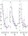 |
Fig. B.3. Similar to Fig. 5, but for a 1 Ms mock X-IFU exposure. |
| In the text | |
Current usage metrics show cumulative count of Article Views (full-text article views including HTML views, PDF and ePub downloads, according to the available data) and Abstracts Views on Vision4Press platform.
Data correspond to usage on the plateform after 2015. The current usage metrics is available 48-96 hours after online publication and is updated daily on week days.
Initial download of the metrics may take a while.