| Issue |
A&A
Volume 682, February 2024
|
|
|---|---|---|
| Article Number | A64 | |
| Number of page(s) | 24 | |
| Section | Planets and planetary systems | |
| DOI | https://doi.org/10.1051/0004-6361/202347391 | |
| Published online | 02 February 2024 | |
Compositional characterization of a primordial S-type asteroid family of the inner main belt★
1
LESIA, Observatoire de Paris, Université Paris Cité, Université PSL, CNRS, Sorbonne Université,
5 place Jules Janssen,
92195
Meudon,
France
2
INAF – Osservatorio Astronomico di Roma,
Via Frascati 33,
00078
Monte Porzio Catone,
Italy
e-mail: jules.bourdelledemicas@inaf.it
3
Institut Universitaire de France (IUF),
1 rue Descartes,
75231
Paris
Cedex 05,
France
4
Université Côte d’Azur, CNRS-Lagrange,
Observatoire de la Côte d’Azur, CS 34229,
06304
Nice
Cedex 4,
France
5
Lowell Observatory,
1400 West Mars Hill Road,
Flagstaff,
AZ
86001,
USA
6
INAF – Osservatorio Astronomico di Padova,
Vicolo dell’Osservatorio 5,
35122
Padova,
Italy
7
Dipartimento di Fisica e Astronomia G. Galilei, Università di Padova,
Vicolo dell’ Osservatorio 3,
35122
Padova,
Italy
Received:
6
July
2023
Accepted:
21
November
2023
Context. Recently, a primordial family of moderate-albedo asteroid fragments was discovered in the inner main belt. Its age was estimated to be 4.4 ± 1.7 Gyr. However, there is a lack of compositional characterization, which is important to the study of the earliest collisions in the main belt.
Aims. In addition to the previously identified members and the parameters that define the family’s borders (V shape), we expanded the list of family members to include asteroids located within the central region of the V shape. These additional potential members were selected based on their diameter (larger than 7 km) and their geometric visible albedo (greater than or equal to 12%). Subsequently, we conducted a spectroscopic survey to determine the dominant taxonomy and composition of this family. This allowed us to further refine the list of family members by removing interlopers.
Methods. From an initial list of 263 asteroids that are considered to be potential members of the aforementioned primordial family, we retrieved their spectra in the visible and near-infrared range from the literature and from the Gala DR3 spectral catalog of Solar System objects. For asteroids with no or poor signal-to-noise ratio spectra in the literature, we carried out new ground-based observations. We obtained new spectra for 33 members of the family using the 1.82 m Asiago Telescope for the visible spectroscopy, while for near-infrared spectroscopy, we used the 3.58 m Telescopio Nazionale Galileo (TNG) and the 4.30 m Lowell Discovery Telescope (LDT).
Results. In total, we collected spectra for 261 potential members of the primordial S-type family out of 263. We determined their spectral taxonomy and properties, such as spectral slopes and absorption band parameters, when existing. Using the taxonomical characterization and the orbital space parameters, we identified and removed 71 interlopers from the potential members list. The final list of the primordial S-type family members includes 190 asteroids. The family is dominated by S-complex (~71%) asteroids with a mineralogy similar to ordinary chondrites and pyroxene-rich minerals. The family also contains members classified as L-types and V-types. (~15% and ~9%, respectively).
Conclusions. The mean albedo of the family is ~23%, and its largest probable remnant is the asteroid (30) Urania. The estimated size of the family parent body ranges between 110 and 210 km. This size range is compatible with the progenitor of H and L chondrites.
Key words: methods: data analysis / methods: observational / methods: statistical / techniques: spectroscopic / minor planets, asteroids: general
New spectra are available at the CDS via anonymous ftp to cdsarc.cds.unistra.fr (130.79.128.5) or via https://cdsarc.cds.unistra.fr/viz-bin/cat/J/A+A/682/A64
© The Authors 2024
 Open Access article, published by EDP Sciences, under the terms of the Creative Commons Attribution License (https://creativecommons.org/licenses/by/4.0), which permits unrestricted use, distribution, and reproduction in any medium, provided the original work is properly cited.
This article is published in open access under the Subscribe to Open model. Subscribe to A&A to support open access publication.
1 Introduction
It is well established that small bodies can preserve relatively unaltered materials (Johansen et al. 2015) that date back to the formation of our Solar System 4.567 Gyr ago, the latter time being established by the formation of the calcium-aluminum- rich inclusions (CAIs), the oldest Solar System condensates (Amelin et al. 2002). Thus, asteroid studies provide us with important clues to fundamental questions regarding solar system formation, such as their contribution in bringing water and organics to Earth (Morbidelli et al. 2000). While some of the asteroids that we observe today could have accreted directly from the protoplanetary disk of our Sun, the majority of them experienced collisional events, leading to the formation of families of asteroid fragments (Nesvorný et al. 2015).
In a breakup process, fragments are launched into space at a moderate velocity (~ 1 km s−1), and in the asteroid belt (but not elsewhere), these fragments keep orbital elements that are similar to that of their parent body. Thus, the fragments themselves become new asteroids that are clustered in orbital space and have similar physical properties, such as geometric visible albedo (pV), colors, and spectra (except for the case of the disruption of a differentiated parent body).
The common method used to detect such clusters is the hierarchical clustering method (HCM; Zappala et al. 1990; Nesvorný et al. 2015). Although very effective, this method appears to have problems detecting very old families (Bolin et al. 2017; Delbo et al. 2017). Indeed, there is evidence of a severe deficit of known families older than 2 Gyr compared to what is expected when assuming a constant asteroid breakup rate over the age of the Solar System (Brož & Morbidelli 2013; Spoto et al. 2015). As a matter of fact, family members have been affected by non-gravitational forces, such as the Yarkovsky effect (Vokrouhlický et al. 2015), causing their orbital semimajor axis to drift over time. Asteroids, as they are affected by this orbital drift, encounter orbital resonances with planets that change their orbital e and i (but not their a). Thus, families become harder to identify as they age because they become increasingly dispersed (Parker et al. 2008) and they overlap each other. Thus, the oldest families of the main belt are highly spread across in orbital elements, making their detection more difficult.
To detect the oldest asteroid families, an alternative method has been developed by taking into account the non-gravitational forces. The so-called V-shape method (Walsh et al. 2013; Bolin et al. 2017; Delbo et al. 2017, 2019) consists of searching for a correlation between the inverse of asteroid diameters  and the proper semimajor axis (a). In this representation, asteroids that are members of a given family are all located within a V shape, with the vertex centered around the largest body of the family, while the sides have lower slope values, as much of the family is old and its smaller members have been spread away in the semimajor axis by non-gravitational forces.
Thanks to this method, very old families have been “dynamically” identified in the inner part of the main belt. For example, Delbo et al. (2017) discovered a primordial low-albedo 4-Gyr- old family; Delbo et al. (2019) detected two X-complex families, Athor and Zita, with ages of 3 and 4.5 Gyr, respectively; and, recently, a primordial family has been detected by Ferrone et al. (2023) among the asteroids of intermediate albedo in the inner main belt. This latter work defined, with a high confidence level, the edges of the V shape and its age (4.4 ± 1.7 Gyr) and identified the family members located close to the edges of the V shape. A preliminary inspection of these members indicated that this primordial family appears tobe formed by S-type asteroids. For this reason, we refer to this family as the primordial S-type family (hereafter, PSTF) throughout this work.
In this work, we carried out spectroscopic surveys in the visible and near-infrared range to determine the composition of the family and to distinguish interlopers from the real members. Section 2 is dedicated to the establishment of the potential PSTF members list, and in Sect. 3, we detail the observing strategy as well as the data reduction and analysis procedures. Section 4 presents the results of the classification in well-established taxonomies and the identification of interlopers. Finally, in Sect. 5, we determine the size distribution of the family members and correct it for collisional and dynamical losses of asteroids over the age of the Solar System in order to reconstruct the original size of the PSTF parent body.
2 Establishment of the list of the potential members
Ferrone et al. (2023) identified the PSTF by using the V-shape searching method (Bolin et al. 2017) but only considered bodies of the inner main belt with a geometric visible albedo above 12%. Before enacting this search, however, the authors reassessed the members of known families in the area, trying to be as inclusive as possible, and removed the known and reassessed families. This improved the detectability of the PSTF, for which these authors reported only 42 bodies with a minimum of a 1-σ detection confidence (corresponding to a minimum membership probability of 68%) near the “lobes” of the family’s V shape.
After having identified families’ V shapes, Ferrone et al. (2023) identified planetesimals (or original) as those asteroids that could not be part of any V shapes, implying that these objects are not fragment asteroids that formed locally from the breakup of a larger (and older) parent. However, there is the possibility that some planetesimals could still be lurking within family V shapes (see Ferrone et al. 2023 for more information).
The first example concerns the asteroids (172) Baucis, (186) Celuta, (234) Barbara, and (337) Devosa. Indeed, these objects were identified as planetesimals by Bourdelle de Micas et al. (2022) and therefore cannot be members of any family in the inner main belt. In addition, Ferrone et al. (2023) only reported the families of Nesvorný et al. (2015) and did not include the Athor and Zita families (Delbo et al. 2019). Hence, along with the aforementioned asteroids, we also removed (161) Athor from the list of potential PSTF members. In order to have the lowest number of false positives, we removed (1365) Henyey and (1419) Danzig as well, which are both considered to be members of the Flora family, according to Nesvorný et al. (2015).
Thus, we kept 35 asteroids from the list of Ferrone et al. (2023), all located around the lobes of the PSTF V shape. Ferrone and co-authors did not provide information about the potential PSTF members located in the core of the family, which is inside the edges of the V shape. We thus generated a list of potential members of the PSTF family by applying the following criteria: (1) Members should have a geometric visible albedo greater than 12 %, as in Ferrone et al. (2023). This allows us to directly exclude objects with a very different composition, such as C-complex asteroids. (2) Members should have a diameter greater than 7 km to distinguish them from background objects, which are dominant at a smaller size. We adopted this limit based on the size distribution reported in the study of Ferrone et al. (2023). (3) Objects should not be members of other known families.
To perform the identification of the potential members of the PSTF, we used the MP3C website1 (Delbo et al. 2022), which we used to retrieve values of diameters and albedo. All the potential members, except asteroids (1598) Paloque and (35709) 1999 FR28, have a reported size and albedo value in the literature. By applying our selection criteria, we identified 263 potential members of the family, including the aforementioned 35 objects previously identified by Ferrone et al. (2023). We find it worth noting that we kept in the list the asteroids (1988) Delores and (2286) Fesenkov, which have diameters smaller than 7 km, since they were explicitly identified as members of the PSTF by Ferrone et al. (2023). The list of potential members of the PSTF is presented in Table A.2.
3 Data acquisition, reduction, and analysis
We investigated the composition of the potential family members using existing spectra published in the literature and new telescopic observations. From the literature, we obtained spectra for 129 out of the 263 objects. Specifically, we found 88 spectra in the visible range (0.50–0.90 μm), 31 spectra in the near-infrared range (0.90–2.40 μm), and 10 spectra that covered both the visible and near-infrared range (0.45–2.50 μm). The sources of the different spectra used for our study are reported in Table A.2.
In addition to the literature data, we conducted new observations of 16 asteroids in the visible range and of 26 in the near-infrared range. Furthermore, we analyzed the spectra of 148 potential members of the PSTF present in the Gaia DR3 (Gaia Collaboration 2023).
In total, we obtained spectra for 261 potential members of the PSTF out of 263. Among these, 66 objects have spectra covering both the visible and near-infrared range, while 195 objects have spectra only in the visible range.
3.1 Ground-based observations
For visible spectroscopy, we carried out observations at the 1.82 m Copernico Telescope in Asiago, Italy. For the nearinfrared spectroscopy, we used the 3.58 m Telescopio Nazionale Galileo (TNG) in La Palma, Spain, and the 4.30 m Lowell Discovery Telescope (LDT) in Flagstaff, USA.
Visible spectra were obtained using the Asiago Faint Object Spectrograph (AFOSC; Tomasella et al. 2016) with a 4.22″ slit width and the low-resolution volume phase holographic (VPH#6) grism. This setup allowed us to obtain spectra from 0.52 to 0.95 μm for 16 asteroids between December 2019 and October 2021.
For near-infrared spectroscopy, we used the Near Infrared High-Throughput Spectrograph (NIHTS; Gustafsson et al. 2021) at the LDT, with a slit width of 1.34″, and the Near Infrared Camera Spectrometer (NICS) at the TNG telescope equipped with a 2″ slit and the low dispersion (30–100 Å pix−1) AMICI prism, covering the 0.80–2.50 μm range. We acquired near-infrared spectra of 26 asteroids.
During each night, we also observed several solar analog stars (hereafter SA stars) in proximity (in time and in position) to the asteroids in order to remove the solar light from the reflected asteroid spectra. Typically, we observed trusted G2V solar analog stars (Hardorp 1978). However, for near-infrared spectroscopic observations, these stars were not always located close enough to the asteroid, which is a necessary condition for proper correction of the telluric features. In such cases, we observed F- or G-type stars that were closer in position to our targets, and applied a color correction, as described in Sect. 3.2.
For near-infrared spectroscopy, we followed the classical ABBA observation procedure, where we alternated observations of the targets at two different slit positions (called A and B, respectively). Each individual observation had a maximum integration time of 2 min, that is, the time in which the atmospheric cells are considered stable enough for a proper correction of telluric features. The ABBA cycles were repeated until the desired signal-to-noise ratio was achieved.
Standard calibrations, including bias, flat-field, and wavelength calibration lamps, were obtained during the daytime before the observations (see Bourdelle de Micas et al. 2022 for details). For the TNG, due to the low dispersion and blending of lines in the calibration lamp, the wavelength calibration was done using a theoretical dispersion table provided by the TNG team2. Observational conditions are reported in Table A.1.
3.2 Data reduction
Spectra obtained with NIHTS were reduced using the SPectral EXtraction Tool (Spextool), an IDL package developed by Cushing et al. (2004). For the reduction of NICS and Afosc data, we used the ESO-Midas package (Banse et al. 1983).
Standard reduction procedures described by Fornasier et al. (1999), 2010) and Bourdelle de Micas et al. (2022) were applied to both the visible and near-infrared data. These included wavelength and flat-field calibrations, as well as cosmic-ray removal. Visible data were also corrected by bias and atmospheric extinction using the extinction table provided by the Asiago observatory website3.
To calculate the reflectance of the asteroids, we divided each asteroid spectrum by that of the solar analog star observed closest in time and airmass to the asteroid. When an F- or G-type star was observed closest in sky position to an asteroid, which mostly occurred in near-infrared spectroscopic observations, we defined the following factor Fc to correct the color of these stars:
 (1)
(1)
where s* corresponds to the signal of the star and sG2V corresponds to the signal of the trusted solar analog. To avoid the contribution of telluric band effects on Fc(λ), we replaced the telluric band residuals by a linear fit of the data around the edges of the band. We also applied a median filter with a large window to reduce the noise and telluric residuals. The relative reflectance of an asteroid R(λ) is given by:
 (2)
(2)
The last step in the reduction process was the normalization of the spectra, which was done at 0.55 μm in the visible range, and at 1.0 μm in the near-infrared range.
Finally, we merged the individual segments of the spectrum, specifically in the visible and near-infrared parts, when available, following the same procedure described by Bourdelle de Micas et al. (2022). First, a superposition region between the two segments, usually between 0.80 and 0.90 μm, was identified, and a common wavelength (λnorm) suitable for normalization was chosen. Then, the reflectance of each segment was averaged in the range λnorm ± 0.02 μm, and each visible and near-infrared spectrum was normalized by the corresponding mean reflectance. Finally, a visual inspection was performed to check if the junction between the two parts respected the apparent continuum of the spectrum in that region, and adjustments were made to the segment normalization if needed.
The complete visible and near-infrared spectrum was finally normalized at 0.55 μm. Due to low signal-to-noise values in the near-infrared range, 17 spectra had to be cut before 2.00 μm because they were too noisy for the analysis at longer wavelengths. The spectra from these new observations are represented in Figs. 1 and 2.
3.3 Gaia data
To extend the spectral investigation to the maximum number of PSTF members, we also inspected the Gaia spectral database of asteroids (DR3; Gaia Collaboration 2023). The European Space Agency (ESA) Gaia mission has observed thousands of asteroids since 2014 using its two low-resolution photometers: the blue photometer (BP), dedicated to short wavelengths (0.325–0.650 μm), and the red photometer (RP) for the longer wavelengths, 0.650–1.125 μm (Gaia Collaboration 2023).
The DR3 spectral catalog contains data of 60 518 asteroids that have been observed between 4 to 80 times. Inner main belt objects have mostly been observed at a phase angle around 20°. In the Gaia catalog, the asteroid spectra are presented in reflectance relative to the Sun and normalized at 0.55 μm. The reflectance is computed as a weighted mean in 16 bands covering the 0.374 and 1.034 μm range, with a bin size of 0.044 μm (Gaia Collaboration 2023), and the associated error is the standard deviation of the spectrophotometry at a given band for the different observations available for a given asteroid. To remove the solar contribution, several solar analog stars have been averaged (Gaia Collaboration 2023).
However, Tinaut-Ruano et al. (2023) recently found a systematic problem in the solar contribution removal process at the shortest wavelengths (the first five bands) in the Gaia DR3 catalog, resulting in a decrease of the asteroid spectral slope in the UV-blue region (between 0.374 and 0.506 μm). Consequently, we applied the correction factors found by Tinaut-Ruano et al. (2023) to the Gaia spectra used in our analysis.
The quality of the spectra in the Gaia database is indicated by a flag for each band, with 0 indicating reliable data, 1 indicating suspicious data, and 2 indicating unreliable data. Upon inspecting the Gaia data, we observed that the first and last bands consistently exhibit anomalous reflectance values compared to the apparent continuum of the spectrum. This phenomenon has also been observed by Gaia Collaboration (2023). Therefore, we decided to exclude these bands as well as the ones flagged 2 from the analysis of the spectra of interest.
The Gaia database includes 148 visible spectra of potential members of the PSTF family.
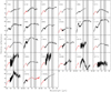 |
Fig. 1 Observed spectra of potential members of the PSTF family. The new observations are presented in black, while spectra from the literature are shown in red. The red points, in the visible range, represent the Gaia data (uncertainties are often within the symbol size). Gray areas correspond to the position of the main telluric absorption bands. The taxonomy presented in this plot is the one we estimated (see Sect. 3.4). |
3.4 Spectral analysis
The first step of our analysis was to classify the spectra following the Bus-DeMeo taxonomy (DeMeo et al. 2009). To do so, we used the M4AST tool4 (Popescu et al. 2012), which compares the spectra of the asteroids with the mean spectra of each Bus-DeMeo class. Using the least chi-squared method, the tool determined the first five classes that best match. Then, we visually inspected the different solutions to identify the best one, that is, the one with similar absorption features to the asteroid and the lowest chi-square value.
For the Gaia data, we observed that the 0.90–1.00 μm band (which is typically found in S-complex spectra, for example) is not systematically well identifiable, especially for fainter asteroids. Therefore, it was often difficult to discriminate between L-type and S-complex (S-, Sa-, Sq-, Sr-, and Sv-types) classifications.
The second step of our analysis consisted of computing the spectral slope in two different spectral ranges by applying a linear fit to the data, as described by Fornasier et al. (2016). Slopes were computed for the entire spectral range and for the visible range between 0.50 and 0.75 μm. Uncertainties were estimated by taking into account the 1σ deviation plus 0.5%/103Å, estimated from the observations of different solar analog stars during a given night, to take into account the spectral variations induced by the use of different stars to remove the solar contribution.
Finally, to characterize absorption bands, we applied the method described by Gaffey et al. (1993) and applied by Bourdelle de Micas et al. (2022). Thus, we first computed the linear continuum at the two edges of the band. Then, we applied a polynomial fit of the nth order, with n comprised between three and eight. The band center was estimated by looking at the wavelength value where the first derivative of the polynomial function is equal to zero. For further information about the characterization of absorption bands, we refer the reader to Bourdelle de Micas et al. (2022).
The data we present were not corrected for the spectral phase reddening (i.e., how the spectral slope varies with the phase angle) for two reasons. Firstly, some data extracted from the literature lack essential information about the phase angle or the observation date. In addition, the Gaia spectra are computed by averaging several observations of a given asteroid acquired at different geometrical conditions (Gaia Collaboration 2023). Therefore, the phase reddening correction cannot be applied to several asteroids of the PSTF. Secondly, we tested the phase reddening correction on the S-type asteroids we observed and found negligible variations that do not affect the taxonomical classification or the mineralogical analysis. Taking all of this into consideration, we decided not to apply the phase reddening correction.
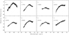 |
Fig. 2 Observed spectra in the visible range of potential members of the PSTF. |
4 Results
4.1 Taxonomy of the potential family members
In Table A.2, we present the results of our taxonomical classification (highlighted in bold) for each member of the family. Additionally, we include the spectral classes determined in the literature whenever available. We observed differences between our classification and that of the literature in only 11.5% of the sample. These differences appear for the L versus S-complex classification and for the D- and T-types versus the X-complex taxonomy.
We are confident in our taxonomical classification because we performed a careful inspection of the spectra, and we combined all the available data to have the widest spectral coverage, while in the literature, the classification of a given object may be derived considering only the visible or the near-infrared range of the spectra. Moreover, we selected as potential members of the family only asteroids with an albedo higher than 12%. With this criterion, it is unlikely to have D-, P- or T-type asteroids in our sample. Therefore, despite the classification given by the literature, we decided to classify these objects as X-types.
The PSTF is dominated by S-complex members, as expected, and includes some X-complex, L-type, and V-type asteroids. In Fig. 3, we present the taxonomy of the potential members in the inverse of the diameter versus semimajor axis plot. We observed that the majority of the potential members belonging to the X-complex are located in the core of the V shape, while the S-complex ones are found both in the core and along the lobes defining the edges of the family. We note that the PSTF is surrounded by and overlaps with other large families, such as the Vesta, dominated by V-type asteroids; the Athor; the Zita; and the Nysa, which are dominated by X-complex asteroids. In defining the borders of the V shape and the core of the family, the known members of the Nysa and Vesta families (Nesvorný et al. 2015) were already excluded (Ferrone et al. 2023).
In Fig. 3, we also present the taxonomy distribution for different sized ranges. The largest potential member of the PSTF is (30) Urania, an S-type asteroid with a diameter of 91.3 ± 0.7 km. The majority of the potential members of the PSTF are relatively small, with diameters ranging from 7 to 10 km, with the addition of the two members with 5 < D < 7 km from Ferrone et al. (2023). The S-complex objects can be observed in each size range, while X-complex members have diameters ranging from 5 to 20 km. Before drawing conclusions on a family’s nature, we needed to identify interlopers as well as to remove them from the list of family members.
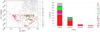 |
Fig. 3 Different distributions of taxonomic classes determined in this study. Left: PSTF’s V shape with taxonomical distribution of its potential members. The V shape presented in this plot (the black line and the dashed lines) is from Ferrone et al. (2023). We refer the reader to that paper for further details regarding the V-shape determination. Right: distribution of the spectral classes of the potential PSTF members per size bin. |
4.2 Identification of interlopers
While we found that the majority of the PSTF members are S- complex asteroids, we also identified that 17% of them belong to the X-complex and 8% are V-types. To explain the presence of other taxonomical types among the asteroids in the family member list, it is important to note that the PSTF, being an old family (with an age estimated to be ≳ 4 Gyr, according to Ferrone et al. 2023), is spread across the entire inner main belt. Therefore, it is highly probable that the potential members list defined earlier includes interlopers or members of other families located in the background. To identify interlopers within the potential PSTF members list, we proceeded as follows.
For a given spectral type or complex, we plotted the V shapes of other known families dominated by that class in an a versus  plane. Additionally, we plotted these families in an orbital space plane, sin(i) versus e. In the latter plot, we identified the regions where the majority of the members are located and drew boxes that characterize these regions.
We included the potential members of the PSTF and its V shape in these plots. By examining the positions of the potential PSTF members, we identified objects located inside the V shape of other families. We considered these asteroids “suspicious” members. Simultaneously, we reported these objects on the orbital elements plot.
If a “suspicious” object was located inside the typical distribution in the sin(i) versus e plane of a given family, we considered it to be an interloper. Otherwise, the object remained in the list of PSTF members.
4.2.1 S-complex
In the inner main belt, there are several families dominated by S-complex asteroids, including Flora, Massalia, Lucienne, Euterpe, Datura, and Lucascavin (Nesvorný et al. 2015).
However, Lucienne, Datura, and Lucascavin families are not included in our analysis because their V shapes are narrow and may be included in the ones of Flora or Baptistina, or within the Nysa-Polana complex. Only the Flora, Massalia, and Euterpe families were considered as potential sources of S-complex interlopers.
In Fig. 4 (left), all S-complex potential members of the PSTF are represented in the a versus  plot. We also represent the V shapes, determined by the C0 value provided by Nesvorný et al. (2015), of the main S-complex families in the inner main belt, namely, Flora, Euterpe, and Massalia. Twenty-two asteroids fall both within the V shape and orbital elements space of the Flora family, and therefore, we consider them to be interlopers of the PSTF. Conversely, asteroids that are within the V shape of the Euterpe and Massalia families are outside the e and sin(i) bounds of Euterpe and Massalia. Therefore, this last set of asteroids cannot be tagged as interlopers of the PSTF (Fig. 4, right panel). We kept this set in the list of potential members of the PSTF.
4.2.2 V-types
We found that 8.43% of potential PSTF members are V-types (Fig. 3). In the inner main belt, the Vesta family is one of the largest families, and it is dominated by V-types (De Sanctis et al. 2012; Nesvorný et al. 2015). Therefore, it could be a source of interlopers for the PSTF.
We followed the same procedure as described earlier to identify interlopers among the V-type potential members. We plotted the V shape of Vesta using the C0 value given by Nesvorný et al. (2015). We display all the V-type potential members of the PSTF in Fig. 5 (top) in red, and those inside the V shape of Vesta are in blue. We considered the asteroids (854) Frostia, (1914) Hartbeespoordam, (2432) Soomana, (2442) Corbett, (2557) Putnam, (2763) Jeans, and (5875) Kuga to be suspicious objects. Next, we plotted them in the sin(i) versus e plane, and we compared their distribution against those of Vesta family members (Fig. 5, bottom). Five out of the seven potential interlopers are within the Vesta family orbital elements space; thus, we ultimately considered them as interlopers. These bodies are (1994) Hartbeespoordam, (2432) Soomana, (2442) Corbett, (2557) Putnam, and (5875) Kuga, and they may be members of Vesta’s family.
4.2.3 X-complex
We found that around 17% of asteroids present in the list of potential PSTF members belong to the X-complex. In the inner main belt, there are primarily two families, Athor and Zita, consisting of X-complex asteroids (Delbo et al. 2019; Avdellidou et al. 2022), and the Nysa-Polana complex has several collisional families that contain X-complex asteroids (Walsh et al. 2013; Dykhuis & Greenberg 2015). In particular, Athor and Zita were discovered by Delbo et al. (2019), who were searching within the population of X-complex asteroids. Subsequent detailed spectroscopic observations revealed that Athor is essentially composed of Xc-type asteroids, while Zita is dominated by Xk- and X-type asteroids (Avdellidou et al. 2022). These families are old, with an estimated age of ~3.0 Gyr and ~4.5 Gyr, respectively (Delbo et al. 2019). Their members are spread across the inner main belt, and therefore the boxes defining the region in sin(iP) and eP occupied by their members contain the entire inner main belt (2.1 < aP < 2.5 au, eP ≲ 0.3, sin iP ≲ 0.3). Nevertheless, the V shapes of Athor and Zita families are still well defined, with a center and slope of aC = 2.38 au and K = 1.72 au−1 km−1, and aC = 2.28 au and K = 1 au−1 km−1, respectively (Delbo et al. 2019). The center of the high albedo component of the Nysa-Polana complex is at aC = 2.42 au, while its slope K ~ 4 au−1 km−1 can be derived from  (Delbo et al. 2017). Its C = 10−4 au, and its average geometric visible albedo pV = 0.28 (Nesvorný et al. 2015). From the extension of the Nysa-Polana complex in the orbital element space, we can take 0.14 < eP < 0.25 and 0.03 < sin iP < 0.07.
We observed that only five asteroids, namely, (620), (647), (1155), (1586), and (14465), are located outside the V shapes and the orbital element box constraints of Athor, Zita, and the Nysa-Polana complex. When examining the albedo value of the five remaining asteroids, (620) Drakonia and (647) Adelgunde have a pv value of 0.42 ± 0.05 and 0.51 ± 0.04, respectively. Consequently, based on the Tholen taxonomy (Tholen 1984), we classified these two asteroids as E-type. Due to the disparity in composition between these asteroids and the S-complex, we chose to exclude them from the list of members. Finally, we considered (1155) Aenna, (1586) Thiele, and (14465) 1993 NB as members of the PSTF, while we identified the other 42 X-complex asteroids as interlopers.
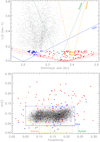 |
Fig. 4 Comparison between the distribution of S-complex PSTF potential members and S-complex background families. Top: V shape of Flora family (in blue) in a plan |

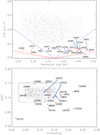 |
Fig. 5 Comparison between the distribution of V-type PSTF members and Vesta’s family. Top: V shape of Vesta family (in blue) and the PSTF (in red). The red and blue points represent potential members of the PSTF that are respectively outside and inside Vesta’s V shape. The black points represent members of the Vesta family. Bottom: distribution in the sin(i) versus eccentricity space of PSTF potential members (in red and blue points) compared to Vesta members. The black rectangle represents the border of the Vesta region in the orbital elements space. |
4.3 The PSTF family after interlopers removal
After excluding interlopers, the list of PSTF members was reduced to 190 asteroids. The identification of confirmed members and interlopers is reported in Table A.2. In Fig. 6, we summarize the main spectral properties and characteristics of the PSTF, which is dominated by S-complex asteroids (~71%) with a non-negligible percentage of L-types (~15%) and V-types (~9%).
From the list of confirmed members, we calculated the spectral slope and analyzed the absorption bands, if present, for either newly observed asteroids or those with available data in the literature.
In Fig. 7, we present the visible spectral slope versus albedo of the potential PSTF members. We plotted the spectral slope computed in the visible range because it is available for all the investigated asteroids, while near-infrared spectra are missing for several bodies.
In this plot, we observed that members of the PSTF are regrouped in an area located at 0.12 < pv < 0.38 and 4 < slope < 23%/1000 Å. There is no clear separation between the different classes. Considering the list of confirmed members defined here, the mean geometric visible albedo of the family is 22.5 ± 2.7 %. As previously indicated, the largest member of the PSTF is the asteroid (30) Urania, which may be the parent body of the PSTF.
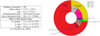 |
Fig. 6 Summary of parameters characterizing the PSTF after exclusions of interlopers. Left: summary of the main characteristics of the PSTF. Right: distribution of the PSTF members taxonomical classes after exclusion of interlopers. |
4.4 Spectral analysis of the PSTF members
The S-complex is characterized by the presence of two bands in the visible and near-infrared range, located at around 1.0 and 2.0 μm (hereafter, BI and BII, respectively). The BI band may be due to the presence of olivine and pyroxene, while the 2.0 μm band is due to pyroxene (Cloutis et al. 1986; Gaffey et al. 1993). The BI and BII band depths may vary among S-complex asteroids, depending on the olivine-pyroxene ratio. Cloutis et al. (1986) defined the band area ratio (hereafter, BAR) as the ratio of the 2.0 pm band area over the 1.0 pm one. Gaffey et al. (1993) established a classification scheme of silicate asteroids considering their distribution in the plane composed of the BI center band position versus the BAR area ratio. Gaffey et al. (1993) defined seven different groups of S-types (numbered S(I) to S(VII)) with varying amounts of olivine and pyroxene abundances. The S(I) group characterizes olivine-rich asteroids, while S(VII) corresponds to pyroxene-dominated objects.
We therefore computed the BI center position and the BAR for the S-type asteroids with a complete visible and near-infrared spectrum (18 asteroids) following the approach described in Gaffey et al. (1993). We computed the linear continuum between the band’s borders for each of the BI and BII bands, and then we divided the extracted spectrum of each band by the associated linear continuum. We applied a polynomial fit of order N, where N ranges between three and eight, and we determined the band parameters using the polynomial best fitting a given band and the uncertainties considering the variations in the parameters using the polynomials N−1 and N+1.
In Fig. 8, we present the S-subclasses, following the Gaffey et al. (1993) classification scheme, for the 18 S-complex asteroids with a complete visible and near-infrared spectrum (18 asteroids). The values of the band parameters are reported in Table A.3. Twelve of them are located in the S(IV) group, corresponding to the S-complex objects with a mineralogy similar to ordinary chondrites (Gaffey et al. 1993; Mothé-Diniz et al. 2005). Two asteroids, (3385) Bronnina and (3920) Aubignan, show an olivine-rich composition and are located in the S(II) region. Conversely, (287) Nephthys, (391) Ingeborg, and (1565) Lemaitre show a mineralogy dominated by pyroxene (S(VII)). Finally, (1589) Fanatica is located in the S(V) region, which is characterized by an equal composition between olivine and pyroxene (Gaffey et al. 1993).
Although the sample size is small, these findings suggest that the PSTF might be dominated by a composition similar to that of ordinary chondrites. This also suggests that it includes, in lower proportion, members rich in pyroxene.
Among the most represented classes, we found that ~9% of members of the PSTF belong to the V-type, which is characterized by deeper 1.0 and 2.0 μm bands compared to S-complex asteroids. Similar to the mineralogical characterization of S- complex asteroids, it is possible to determine the mineralogical properties of V-types based on their absorption band features. It is well known, thanks notably to the results from the Dawn mission, that (4) Vesta (the largest V-type asteroid of the main belt) is the parent body of the howardite, eucrite, and diogenite (the so-called HED) meteorites (McSween et al. 2013). Therefore, we followed the approach of Moskovitz et al. (2010), which involves plotting V-type asteroids on the BI center versus BII center plane and comparing their distribution with the regions characteristic of the diogenite, howardite, and eucrite mineralogies (gray rectangles in Fig. 9). To compare the location of the members of the PSTF with Vesta (and its family by extension), it is important to consider that Vesta shows significant variations in terms of band center positions, indicating compositional heterogeneity (Gaffey 1997). To make this comparison, we identified an area, from De Sanctis et al. (2012), that corresponds to different observations of Vesta’s surface during the surface orbital stage of the Dawn spacecraft. To draw this box, we considered all observations and their uncertainties. The result is presented in Fig. 9, and the computed BI and BII center values are presented in Table A.4.
In Fig. 9, we observed that four asteroids, (2371) Dimitrov, (2653) Principia, (2763) Jeans, and (2851) Harbin, are located within the mixed area define by howardites and eucrites. The (2168) Swope and (2566) Kirghizia asteroids are located close to these regions but are not within them. This shift has been reported previously in the literature and has been interpreted as an effect of regolith grain size or space weathering (Duffard et al. 2005; Moskovitz et al. 2010). Thus, we can assume that these objects likely have a howardite- or eucrite-dominated mineralogy. Although (4302) Markeev appears to be far from the HED mineralogical space, there are significant uncertainties in the BI band center position, which was determined using Gaia spectrophotometry.
Except for (854) Frostia and (4302) Markeev, all studied V-type members are located within the Vesta region. This result suggests that the majority of the V-type members in the PSTF share the same composition as Vesta.
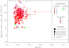 |
Fig. 7 Distribution of potential PSTF members in a visible spectral slope versus albedo plan. The size of the symbols is proportional to the asteroid diameter. |
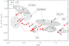 |
Fig. 8 Distribution of potential S-complex members of the PSTF in the BI center versus BAR ratio plan. The ellipses represent the subgroups defined by Gaffey et al. (1993). The abbreviation Ol stands for monomineralic olivine; Capx is calciopyroxene; OC is mafic silicate components of ordinary chondrites; and Opx is orthopyroxene. |
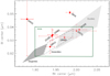 |
Fig. 9 Distribution of potential V-type members of the PSTF in a BI center versus BII center plan. From left to right, the gray areas correspond to the regions of diogenite, howardite, and eucrite mineralogies. The green square corresponds to the space where Vesta is located when considering its variability during multiple observations, according to De Sanctis et al. (2012) and McCoy et al. (2015). |
5 Discussion
5.1 Size distribution
We computed the size distribution of the asteroids in the list of confirmed members of the PSTF (Fig. 10). Since the family is billions of years old, its size distribution can be expected to have been affected by substantial erosion of objects due to their collisional (Bottke et al. 2005) and dynamical evolution (see also Delbo et al. 2017).
We first estimated the size-dependent probability that PSTF members were dynamically removed from main belt. For this, we used the simulations performed by Delbo et al. (2017) of the orbital evolution of a randomized synthetic asteroid population in the inner main belt. We expressed their results by a function, Eq. (3), giving the probability, p(D), as a function of the asteroid’s diameter, D, that this body left the main belt after 4 Gyr of orbital evolution:
 (3)
(3)
Next, we performed a Monte Carlo simulation where for each asteroid member of the PSTF, we extracted a random number from a uniform distribution between one and zero, and we eliminated the asteroid if said number was smaller than the asteroid’s corresponding P(D) value, as calculated from Eq. (3). This procedure resulted in an erosion of the size frequency distribution (SFD) of the PSTF. We then applied a second SFD erosional step to simulate the elimination of asteroids due to collisions. For this, we adopted a classical method that consists of determining the probability that an asteroid undergoes a catastrophic collision during a time ∆t. This probability is equal to the sizedependent inverse collisional lifetime from Bottke et al. (2005) multiplied by the time ∆t. Subsequently, a Monte Carlo simulation was run for a number of steps equal to 4.4 Gyr/∆t and for 10 Gyr/∆t (where ∆t = 10 Myr). At each step an asteroid was eliminated from the simulation if a random number, uniformly distributed between zero and one, was found to be smaller than that probability. We carried out this entire process 301 times for each member of the PSTF, and we estimated its average loss rate and its standard deviation. Finally, we calculated the corrected cumulative SFD of the PSTF by adding the inverse of the average loss rate while counting asteroids in the order from largest to smallest in size. In Fig. 10, we present an SFD correction assuming two collisional evolution models: one model assumes the current state of the solar system for the entire simulation, and the other takes into account that the collisional loss was greater in the earlier days of the Solar System. The collisional loss is expected to decrease as a function of time since the main belt contains fewer bodies for other bodies to collide into. To compensate for this, Bottke et al. (2005) estimated that prolonging the total time 10 Gyr in the current state of the solar system is roughly equivalent to integrating for 4.5 Gyr in a solar system that experienced higher collisional loss in its earlier days. It is common to assume that cumulative SFDs of families can be approximated by a power law (Durda et al. 2007; Masiero et al. 2013) represented by Eq. (4):
 (4)
(4)
where N is the number of asteroids larger than D, N0 is the cumulative number of objects with D ≥ 1 km, and α is the cumulative slope. We fit Eq. (4), by means of the free parameters N0 and α, to the observed and the corrected SFDs, considering asteroids with diameters between 9 and 40 km only. Namely, we avoided the end of the size distribution containing the largest objects because their number is stochastic, that is, there are few objects, and their sizes could be affected by the highly variable impact geometry of the projectile on the family’s parent body. We also avoided the small end of the SFD because it is necessarily observationally incomplete. Typically, family SFDs are fit in the regime where collisional fragmentation is thought to dominate and the sample is complete, which in our case is safe to assume in the range 9 ≲ D ≲ 40 km. We obtained α values ranging between −1.8 and −2.8. The former and the latter values correspond, respectively, to α values derived by fitting Eq. (4) to the observed SFD and the SFD corrected for the highest dynamical and collisional loss (10 Gyr; Fig. 10).
The initial size of the PSTF can be determined by integrating Eq. (4), that is:
 (5)
(5)
where Vp is the volume of the family precursor body and DMax = N010−α is the largest object on the power-law SFD. Equation (5) can be solved analytically for αini > −3, which is our case; thus,
 (6)
(6)
yielding the diameter of the PSTF family progenitor to be between ~ 110 and ~ 210 km.
This diameter range is compatible with the H and L chondrite planetesimal sizes inferred from thermal modeling of thermochronometers inside the ordinary chondrites (Trieloff et al. 2003; Gail & Trieloff 2019). This is contrary to the case of the EL enstatite chondrites where their source family progenitor (Avdellidou et al. 2022) is much smaller than the size of the planetesimal within which these meteorites formed (Trieloff et al. 2022), possibly indicating that the EL planetesimal broke outside the main belt and that a fragment of it, the source family progenitor, was implanted into the main belt by some dynamical process (Avdellidou et al. 2022). Hence, we speculate that the parent body of the PSTF could have accreted in the main belt.
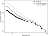 |
Fig. 10 Size distribution of the PSTF members. |
5.2 Comparison with Flora family
We compared the PSTF properties with those of other S-complex dominated families. In the inner main belt, there are seven known families dominated by S-complex asteroids (Nesvorný et al. 2015). However, three of them (Lucienne, Datura, and Lucascavin) have only a small number of members; one, Phocaea, has a very different average inclination (i > 17°); and two have no or little spectroscopic data available (Massalia and Euterpe). Conversely, Flora is a well-known family that has been spectroscopically studied by Oszkiewicz et al. (2015).
As stated earlier, Flora is the biggest S-complex family of the inner main belt, with more than 13 000 members (Nesvorný et al. 2015). Spectroscopic studies have shown that this family contains mainly S-complex asteroids but also a non-negligible number ofL- and V-types (Oszkiewicz et al. 2015). In their work, the authors considered a sample of 2500 members of Flora’s family, and they estimated their taxonomic classes through photometric data (Oszkiewicz et al. 2014). Flora has a lower percentage of S-complex (47.8%) asteroids (Oszkiewicz et al. 2015) compared to the PSTF family (71.1%). This difference may be attributable to the several C-complex and D-type asteroids included in their survey, types that are automatically excluded from the PSTF member list because of their low albedo (we applied the criterion albedo >12% to identify the members of the family). Without the low-albedo bodies, Flora should have ~54% of S-complex, ~9% of X-complex, and ~37% of End members. This result is closer to what we found for the PSTF.
We also observed that the percentage of L-type asteroids is quite similar in the two families (~15%). However, in both studies, the spectra were acquired mostly in the visible region (up to 1.1 μm for the best cases). Near-infrared spectroscopy will be very helpful to fully discriminate L-type from S-complex asteroids, especially in cases like our study where only objects from the Gaia DR3 catalog are used.
When examining the taxonomic distribution of members within the Flora family, we noted that V-type asteroids are present up to 6.6%. Consequently, we expected to find V-type asteroids among the members of the PSTF with a similar proportion (9.0%). However, as our interloper identification may include some false positive results, V-type asteroids may be, in reality, members of the Vesta family.
Finally, we found a smaller number of X-complex PSTF members compared to the Flora family (1.6% against 7.5%). It is probable that this 7.5% should contain members of X-complex dominated families (Athor and Zita) that have not been discovered at the time of the study of Oszkiewicz et al. (2015). However, for the X-type asteroids, the comparison should be done with caution because we might have been too restrictive in X-complex member identification. This is because we considered 4-Gyr-old X-complex families (such as Athor and Zita) that are spread across the entire inner main belt. It could be possible that, in reality, the PSTF contains more X-complex asteroids among its members.
6 Conclusions
After the detection by Ferrone et al. (2023) of a PSTF in the inner main belt, we conducted a spectroscopic analysis of potential members of that family. We initially enhanced Ferrone et al.’s list of members located within the lobes of the PSTF’s V shape by including objects in the “core” of the family. This resulted in a list of 263 potential members of the PSTF. Spectroscopic data were retrieved from new ground-based observations, literature, and the Gaia mission asteroid spectral catalog, covering the visible and, when existing, the near-infrared range. Consequently, we obtained the spectra of about 261 potential members of this family.
In our work, we first performed taxonomic classification on PSTF members. As expected, the family is predominantly composed of S-complex asteroids. However, the significant presence of X-complex, L-type, and V-type objects among the members of the family raised questions regarding their membership. Therefore, we did a more detailed analysis to determine if these objects were members of the PSTF or interlopers. By examining S-complex, V-type, and X-complex objects individually and comparing their orbital characteristics to both PSTF members and background family members, we identified 24 S-complex asteroids that are interlopers of the PSTF (they can be members of the Flora family), five V-types that are interlopers (and potentially members of Vesta’s family), and 42 X-complex asteroids that are also interlopers. The latter can be members of the Nysa complex family, Athor family, or Zita family.
Based on our findings, the list of PSTF members was reduced to 190 objects. From that list and through our studies, we obtained the following results:
The mean albedo value of the family members was estimated tobe 22.72 ± 2.76%;
The S-complex asteroids dominate the family (~70%), followed by L- and V-types (~15% and ~9%, respectively). For the S-complex, we observed a composition similar to that of the ordinary chondrites;
Among the members of the PSTF, approximately 9% are V-types. These asteroids exhibit a composition close to the howardite and eucrite meteorites. However, due to the limited sample considered in this analysis, no definitive conclusions could be drawn regarding general trends for either case;
Through the size distribution of the PSTF, we estimated the size of the parent body of this family, and it ranges between 110 and 210 km. This size range is compatible with the progenitor of H and L chondrites. Among the members of the PSTF, (30) Urania is the biggest (D ~ 91 km). This asteroid could be the parent body of the PSTF;
We compared the taxonomical distribution of the PSTF with that of Flora, another large S-complex dominated family in the inner main belt. In general, we found a distribution that was similar but with a notable exception: the case of X-complex members. Indeed, we found a lower percentage of X-complex PSTF members (~2.6%) compared to Flora (~7.5%). We explain that difference by the fact that our interloper identification could be too restrictive.
Based on the dynamical detection conducted by Ferrone et al. (2023), our spectroscopic study allowed us to include the PSTF to the list of S-complex families present in the inner main belt. Given its presence in this region, itis likely that some S-complex near-Earth asteroids originating from this family will be found in future studies.
Acknowledgements
We acknowledge support from the ANR-ORIGINS (ANR- 18-CE31-13-0014). This work made use of observations collected at the Copernico telescope (Asiago, Italy) of the Istituto Nazionale di Astrofisica (INAF) – Osservatorio Astronomico di Padova, at the Italian Telescopio Nazionale Galileo (TNG) operated on the island of La Palma, Spain, and at the Lowell Discovery Telescope at Lowell Observatory. Lowell is a private, non-profit institution dedicated to astrophysical research and public appreciation of astronomy and operates the LDT in partnership with Boston University, the University of Maryland, the University of Toledo, Northern Arizona University and Yale University. This work is based on data provided by the Minor Planet Physical Properties Catalogue (MP3C) of the Observatoire de la Côte d’Azur. This work has made use of data from the European Space Agency (ESA) mission Gaia (https://www.cosmos.esa.int/gaia), processed by the Gaia Data Processing and Analysis Consortium (DPAC, https://www.cosmos.esa.int/web/gaia/dpac/consortium). Funding for the DPAC has been provided by national institutions, in particular the institutions participating in the Gaia Multilateral Agreement. This research has made use of the Small Bodies Data Ferret (https://sbnapps.psi.edu/ferret/), supported by the NASA Planetary System. Part of the data utilized in this publication were obtained and made available by the MITHNEOS MIT-Hawaii Near-Earth Object Spectroscopic Survey. We thank the anonymous referee for all the comments and suggestions which helped us to improve this article.
Appendix A Tables
Observational conditions of PSTF’s members whose spectra were acquired by the Copernico, TNG, and LDT telescopes.
PSTF potential members list.
Band parameter values for S-complex members of the PSTF. Only the 18 objects with a fully visible and near-infrared spectra were analyzed.
Band parameter values for V-type members of the PSTF. Only objects with a fully visible and near-infrared spectra were analyzed.
Appendix B Figures
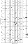 |
Fig. B.1 Visible and near-infrared spectra from literature. Gray areas correspond to the telluric absorption bands. |
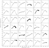 |
Fig. B.2 Visible spectra of the studied potential members of the PSTF. The dotted spectra correspond to the data from the Gaia database. |
References
- Amelin, Y., Krot, A. N., Hutcheon, I. D., & Ulyanov, A. A. 2002, Science, 297, 1678 [NASA ADS] [CrossRef] [Google Scholar]
- Avdellidou, C., Delbo, M., Morbidelli, A., et al. 2022, A&A, 665, A9 [NASA ADS] [CrossRef] [EDP Sciences] [Google Scholar]
- Banse, K., Crane, P., Grosbol, P., et al. 1983, The Messenger, 31, 26 [NASA ADS] [Google Scholar]
- Bell, J. F., Owensby, P. D., Hawke, B. R., et al. 2005, NASA Planetary Data System, EAR-A-RDR-3-52COLOR-V2.1 [Google Scholar]
- Binzel, R. P., Rivkin, A. S., Stuart, J. S., et al. 2004, Icarus, 170, 259 [NASA ADS] [CrossRef] [Google Scholar]
- Binzel, R. P., DeMeo, F. E., Turtelboom, E. V., et al. 2019, Icarus, 324, 41 [Google Scholar]
- Bolin, B. T., Delbo, M., Morbidelli, A., & Walsh, K. J. 2017, Icarus, 282, 290 [CrossRef] [Google Scholar]
- Bottke, W. F., Durda, D. D., Nesvorný, D., et al. 2005, Icarus, 179, 63 [Google Scholar]
- Bourdelle de Micas, J., Fornasier, S., Avdellidou, C., et al. 2022, A&A, 665, A83 [NASA ADS] [CrossRef] [EDP Sciences] [Google Scholar]
- Brož, M., & Morbidelli, A. 2013, Icarus, 223, 844 [CrossRef] [Google Scholar]
- Burbine, T. H., & Binzel, R. P. 2002, Icarus, 159, 468 [CrossRef] [Google Scholar]
- Bus, S. J., & Binzel, R. P. 2002, Icarus, 158, 146 [Google Scholar]
- Cloutis, E. A., Gaffey, M. J., Jackowski, T. L., & Reed, K. L. 1986, J. Geophys. Res., 91, 11, 641 [NASA ADS] [Google Scholar]
- Cushing, M. C., Vacca, W. D., & Rayner, J. T. 2004, PASP, 116, 362 [NASA ADS] [CrossRef] [Google Scholar]
- Delbo, M., Walsh, K., Bolin, B., Avdellidou, C., & Morbidelli, A. 2017, Science, 357, 1026 [NASA ADS] [CrossRef] [Google Scholar]
- Delbo, M., Avdellidou, C., & Morbidelli, A. 2019, A&A, 624, A69 [NASA ADS] [CrossRef] [EDP Sciences] [Google Scholar]
- Delbo, M., Avdellidou, C., Bruot, N., & Erard, S. 2022, in 16th Eur. Planet. Sci. Congress, EPSC2022-323 [Google Scholar]
- DeMeo, F. E., Binzel, R. P., Slivan, S. M., & Bus, S. J. 2009, Icarus, 202, 160 [Google Scholar]
- De Sanctis, M. C., Ammannito, E., Capria, M. T., et al. 2012, Science, 336, 697 [NASA ADS] [CrossRef] [Google Scholar]
- Duffard, R., Lazzaro, D., & de León, J. 2005, J. Maps, 40, 445 [NASA ADS] [Google Scholar]
- Durda, D. D., Bottke, W. F., Nesvorný, D., et al. 2007, Icarus, 186, 498 [NASA ADS] [CrossRef] [Google Scholar]
- Dykhuis, M. J., & Greenberg, R. 2015, Icarus, 252, 199 [NASA ADS] [CrossRef] [Google Scholar]
- Ferrone, S., Delbo, M., Avdellidou, C., et al. 2023, A&A, 676, A5 [NASA ADS] [CrossRef] [EDP Sciences] [Google Scholar]
- Fieber-Beyer, S. K., & Gaffey, M. J. 2015, Icarus, 257, 113 [NASA ADS] [CrossRef] [Google Scholar]
- Fornasier, S., Lazzarin, M., Barbieri, C., & Barucci, M. A. 1999, A&AS, 135, 65 [NASA ADS] [CrossRef] [EDP Sciences] [Google Scholar]
- Fornasier, S., Migliorini, A., Dotto, E., & Barucci, M. A. 2008, Icarus, 196, 119 [NASA ADS] [CrossRef] [Google Scholar]
- Fornasier, S., Clark, B. E., Dotto, E., et al. 2010, Icarus, 210, 655 [NASA ADS] [CrossRef] [Google Scholar]
- Fornasier, S., Lantz, C., Perna, D., et al. 2016, Icarus, 269, 1 [CrossRef] [Google Scholar]
- Gaffey, M. J. 1997, Icarus, 127, 130 [NASA ADS] [CrossRef] [Google Scholar]
- Gaffey, M. J., Bell, J. F., Brown, R. H., et al. 1993, Icarus, 106, 573 [NASA ADS] [CrossRef] [Google Scholar]
- Gaia Collaboration (Galluccio, L., et al.) 2023, A&A, 674, A35 [NASA ADS] [CrossRef] [EDP Sciences] [Google Scholar]
- Gail, H.-P., & Trieloff, M. 2019, A&A, 628, A77 [NASA ADS] [CrossRef] [EDP Sciences] [Google Scholar]
- Gustafsson, A., Moskovitz, N., Cushing, M. C., et al. 2021, PASP, 133, 035001 [NASA ADS] [CrossRef] [Google Scholar]
- Hardersen, P. S. 2016, NASA Planetary Data System, EAR-A-I0046-3-HARDERSENSPEC-V1.0 [Google Scholar]
- Hardersen, P. S., Reddy, V., & Roberts, R. 2015, ApJS, 221, 19 [NASA ADS] [CrossRef] [Google Scholar]
- Hardorp, J. 1978, A&A, 63, 383 [NASA ADS] [Google Scholar]
- Johansen, A., Jacquet, E., Cuzzi, J. N., Morbidelli, A., & Gounelle, M. 2015, in Asteroids IV, eds. P. Michel, F. E. DeMeo, & W. F. Bottke (Tucson: University of Arizona Press) 471 [Google Scholar]
- Lazzaro, D., Angeli, C. A., Carvano, J. M., et al. 2004, Icarus, 172, 179 [NASA ADS] [CrossRef] [Google Scholar]
- Lindsay, S. S., Marchis, F., Emery, J. P., Enriquez, J. E., & Assafin, M. 2015, Icarus, 247, 53 [NASA ADS] [CrossRef] [Google Scholar]
- Masiero, J. R., Mainzer, A. K., Bauer, J. M., et al. 2013, ApJ, 770, 7 [Google Scholar]
- McCoy, T. J., Beck, A. W., Prettyman, T. H., & Mittlefehldt, D. W. 2015, Chem. Erde/Geochemistry, 75, 273 [NASA ADS] [Google Scholar]
- McSween, H. Y., Binzel, R. P., de Sanctis, M. C., et al. 2013, J. Maps, 48, 2090 [NASA ADS] [Google Scholar]
- Morbidelli, A., Chambers, J., Lunine, J. I., et al. 2000, J. Maps, 35, 1309 [NASA ADS] [Google Scholar]
- Moskovitz, N. A., Willman, M., Burbine, T. H., Binzel, R. P., & Bus, S. J. 2010, Icarus, 208, 773 [NASA ADS] [CrossRef] [Google Scholar]
- Mothé-Diniz, T., Roig, F., & Carvano, J. M. 2005, Icarus, 174, 54 [CrossRef] [Google Scholar]
- Nesvorný, D., Brož, M., & Carruba, V. 2015, in Asteroids IV, eds. P. Michel, F. E. DeMeo, & W. F. Bottke (Tucson: University of Arizona Press) 297 [Google Scholar]
- Oszkiewicz, D. A., Kwiatkowski, T., Tomov, T., et al. 2014, A&A, 572, A29 [NASA ADS] [CrossRef] [EDP Sciences] [Google Scholar]
- Oszkiewicz, D., Kankiewicz, P., Wlodarczyk, I., & Kryszczynska, A. 2015, A&A, 584, A18 [NASA ADS] [CrossRef] [EDP Sciences] [Google Scholar]
- Parker, A., Ivezic, Ž., Juric, M., et al. 2008, Icarus, 198, 138 [NASA ADS] [CrossRef] [Google Scholar]
- Perna, D., Barucci, M. A., Fulchignoni, M., et al. 2018, Planet. Space Sci., 157, 82 [CrossRef] [Google Scholar]
- Popescu, M., Birlan, M., & Nedelcu, D. A. 2012, A&A, 544, A130 [NASA ADS] [CrossRef] [EDP Sciences] [Google Scholar]
- Reddy, V., & Sanchez, J. A. 2016, NASA Planetary Data System, EAR-A-I0046-3-REDDYMBSPEC-V1.0 [Google Scholar]
- Reddy, V., Sanchez, J. A., Nathues, A., et al. 2012, Icarus, 217, 153 [NASA ADS] [CrossRef] [Google Scholar]
- Spoto, F., Milani, A., & Kneževic, Z. 2015, Icarus, 257, 275 [NASA ADS] [CrossRef] [Google Scholar]
- Sunshine, J. M., Bus, S. J., Corrigan, C. M., McCoy, T. J., & Burbine, T. H. 2007, J. Maps, 42, 155 [NASA ADS] [Google Scholar]
- Tholen, D. J. 1984, PhD thesis, University of Arizona, USA [Google Scholar]
- Tinaut-Ruano, F., Tatsumi, E., Tanga, P., et al. 2023, A&A, 669, A14 [NASA ADS] [CrossRef] [EDP Sciences] [Google Scholar]
- Tomasella, L., Benetti, S., Chiomento, V., et al. 2016, OAPD Tech. Rep., http://hdl.handle.net/20.500.12386/749 [Google Scholar]
- Trieloff, M., Jessberger, E. K., Herrwerth, I., et al. 2003, Nature, 422, 502 [NASA ADS] [CrossRef] [Google Scholar]
- Trieloff, M., Hopp, J., & Gail, H.-P. 2022, Icarus, 373, 114762 [NASA ADS] [CrossRef] [Google Scholar]
- Vokrouhlický, D., Bottke, W. F., Chesley, S. R., Scheeres, D. J., & Statler, T. S. 2015, in Asteroids IV, eds. P. Michel, F. E. DeMeo, & W. F. Bottke (Tucson: University of Arizona Press) 509 [Google Scholar]
- Walsh, K. J., Delbó, M., Bottke, W. F., Vokrouhlický, D., & Lauretta, D. S. 2013, Icarus, 225, 283 [NASA ADS] [CrossRef] [Google Scholar]
- Xu, S., Binzel, R. P., Burbine, T. H., & Bus, S. J. 1995, Icarus, 115, 1 [NASA ADS] [CrossRef] [Google Scholar]
- Zappala, V., Cellino, A., Farinella, P., & Knezevic, Z. 1990, AJ, 100, 2030 [CrossRef] [Google Scholar]
All Tables
Observational conditions of PSTF’s members whose spectra were acquired by the Copernico, TNG, and LDT telescopes.
Band parameter values for S-complex members of the PSTF. Only the 18 objects with a fully visible and near-infrared spectra were analyzed.
Band parameter values for V-type members of the PSTF. Only objects with a fully visible and near-infrared spectra were analyzed.
All Figures
|
Fig. 1 Observed spectra of potential members of the PSTF family. The new observations are presented in black, while spectra from the literature are shown in red. The red points, in the visible range, represent the Gaia data (uncertainties are often within the symbol size). Gray areas correspond to the position of the main telluric absorption bands. The taxonomy presented in this plot is the one we estimated (see Sect. 3.4). |
| In the text | |
|
Fig. 2 Observed spectra in the visible range of potential members of the PSTF. |
| In the text | |
|
Fig. 3 Different distributions of taxonomic classes determined in this study. Left: PSTF’s V shape with taxonomical distribution of its potential members. The V shape presented in this plot (the black line and the dashed lines) is from Ferrone et al. (2023). We refer the reader to that paper for further details regarding the V-shape determination. Right: distribution of the spectral classes of the potential PSTF members per size bin. |
| In the text | |
|
Fig. 4 Comparison between the distribution of S-complex PSTF potential members and S-complex background families. Top: V shape of Flora family (in blue) in a plan |
| In the text | |
|
Fig. 5 Comparison between the distribution of V-type PSTF members and Vesta’s family. Top: V shape of Vesta family (in blue) and the PSTF (in red). The red and blue points represent potential members of the PSTF that are respectively outside and inside Vesta’s V shape. The black points represent members of the Vesta family. Bottom: distribution in the sin(i) versus eccentricity space of PSTF potential members (in red and blue points) compared to Vesta members. The black rectangle represents the border of the Vesta region in the orbital elements space. |
| In the text | |
|
Fig. 6 Summary of parameters characterizing the PSTF after exclusions of interlopers. Left: summary of the main characteristics of the PSTF. Right: distribution of the PSTF members taxonomical classes after exclusion of interlopers. |
| In the text | |
|
Fig. 7 Distribution of potential PSTF members in a visible spectral slope versus albedo plan. The size of the symbols is proportional to the asteroid diameter. |
| In the text | |
|
Fig. 8 Distribution of potential S-complex members of the PSTF in the BI center versus BAR ratio plan. The ellipses represent the subgroups defined by Gaffey et al. (1993). The abbreviation Ol stands for monomineralic olivine; Capx is calciopyroxene; OC is mafic silicate components of ordinary chondrites; and Opx is orthopyroxene. |
| In the text | |
|
Fig. 9 Distribution of potential V-type members of the PSTF in a BI center versus BII center plan. From left to right, the gray areas correspond to the regions of diogenite, howardite, and eucrite mineralogies. The green square corresponds to the space where Vesta is located when considering its variability during multiple observations, according to De Sanctis et al. (2012) and McCoy et al. (2015). |
| In the text | |
|
Fig. 10 Size distribution of the PSTF members. |
| In the text | |
|
Fig. B.1 Visible and near-infrared spectra from literature. Gray areas correspond to the telluric absorption bands. |
| In the text | |
|
Fig. B.2 Visible spectra of the studied potential members of the PSTF. The dotted spectra correspond to the data from the Gaia database. |
| In the text | |
Current usage metrics show cumulative count of Article Views (full-text article views including HTML views, PDF and ePub downloads, according to the available data) and Abstracts Views on Vision4Press platform.
Data correspond to usage on the plateform after 2015. The current usage metrics is available 48-96 hours after online publication and is updated daily on week days.
Initial download of the metrics may take a while.