| Issue |
A&A
Volume 624, April 2019
|
|
|---|---|---|
| Article Number | A69 | |
| Number of page(s) | 21 | |
| Section | Planets and planetary systems | |
| DOI | https://doi.org/10.1051/0004-6361/201834745 | |
| Published online | 11 April 2019 | |
Ancient and primordial collisional families as the main sources of X-type asteroids of the inner main belt★
1
Observatoire de la Côte d’Azur, CNRS–Lagrange, Université Côte d’Azur,
CS 34229, 06304 Nice Cedex 4, France
e-mail: This email address is being protected from spambots. You need JavaScript enabled to view it.
2
Science Support Office, Directorate of Science, European Space Agency, Keplerlaan 1,
2201 AZ Noordwijk ZH, The Netherlands
Received:
29
November
2018
Accepted:
26
January
2019
Abstract
Aims. The near-Earth asteroid population suggests the existence of an inner main belt source of asteroids that belongs to the spectroscopic X complex and has moderate albedos. The identification of such a source has been lacking so far. We argue that the most probable source is one or more collisional asteroid families that have escaped discovery up to now.
Methods. We apply a novel method to search for asteroid families in the inner main-belt population of asteroids belonging to the X complex with moderate albedo. Instead of searching for asteroid clusters in orbital element space, which could be severely dispersed when older than some billions of years, our method looks for correlations between the orbital semimajor axis and the inverse size of asteroids. This correlation is the signature of members of collisional families that have drifted from a common centre under the effect of the Yarkovsky thermal effect.
Results. We identify two previously unknown families in the inner main belt among the moderate-albedo X-complex asteroids. One of them, whose lowest numbered asteroid is (161) Athor, is ~3 Gyr old, whereas the second one, whose lowest numbered object is (689) Zita, could be as old as the solar system. Members of this latter family have orbital eccentricities and inclinations that spread them over the entire inner main belt, which is an indication that this family could be primordial, that is, it formed before the giant planet orbital instability.
Conclusions. The vast majority of moderate-albedo X-complex asteroids of the inner main belt are genetically related, as they can be included into a few asteroid families. Only nine X-complex asteroids with moderate albedo of the inner main belt cannot be included in asteroid families. We suggest that these bodies formed by direct accretion of the solids in the protoplanetary disc, and are thus surviving planetesimals.
Key words: minor planets, asteroids: general / astronomical databases: miscellaneous
This work is dedicated to the memory of Andrea Milani, who put the foundation and devoted his scientific career on the study of asteroid families.
© M. Delbo et al. 2019
 Open Access article, published by EDP Sciences, under the terms of the Creative Commons Attribution License (http://creativecommons.org/licenses/by/4.0), which permits unrestricted use, distribution, and reproduction in any medium, provided the original work is properly cited.
1 Introduction
Collisions in the asteroid main belt are responsible for sculpting the size distribution of these bodies (Bottke et al. 2015a), forming craters on their surfaces, producing fresh regolith (Hörz & Cintala 1997; Basilevsky et al. 2015), ejecting asteroid material into space (Jewitt et al. 2011), and also implanting exogenous materials (McCord et al. 2012; Avdellidou et al. 2018, 2017, 2016; Turrini et al. 2016; Vernazza et al. 2017).
The most energetic impacts can eject asteroid fragments at speeds larger than the gravitational escape velocity of the parent body. This process can form families of daughter asteroids initially placed on orbits that group near that of the parent asteroid (Zappala et al. 1984). Asteroid families can therefore be recognised as clusters of bodies in proper orbital element space – proper semimajor axis, proper eccentricity, and proper inclination (a, e, i) – with significant contrast with respect to the local background (Milani et al. 2014; Nesvorný et al. 2015). The hierarchical clustering method (HCM; Zappalà et al. 1990; Nesvorný et al. 2015, and references therein) is typically used for the identification of these asteroid clusters.
However, family members disperse with time. Dispersion is driven by a change in the a-value (da/dt ≠ 0) due to the thermal radiation force of the Yarkovsky effect (Vokrouhlický et al. 2006); the eccentricity and inclination are affected by orbital resonances with the planets, the locations of which are crossed by the asteroids as they drift in semimajor axis. This process has fundamental consequences: families older than ~2 Gyr tend to lose number density contrast with respect to the local background population (Parker et al. 2008; Spoto et al. 2015; Carruba et al. 2016). They become more difficult to detect using the HCM compared to younger ones (Walsh et al. 2013; Bolin et al. 2017; Delbo et al. 2017). In addition to the effect of orbital resonances currently present in the main belt, the scattering of fragments of primordial families (Milani et al. 2017, 2014; Delbo et al. 2017) was also affected by major dynamical events such as the giant planet orbital instability, which is shown to have happened at some point in the solar system history (Morbidelli et al. 2015). This latter instability shifted the positions of the resonances and resulted in the incoherent dispersion of e and i of any pre-existing primordial asteroid family in the main belt (Brasil et al. 2016), as is the case for the family of low-albedo asteroids found by Delbo et al. (2017) in the inner main belt (i.e. 2.1 < a < 2.5 au).
The sign of da/dt depends on the obliquity of the spin vector of the asteroid, with prograde-rotating asteroids drifting with da/dt > 0 and retrograde ones with da/dt < 0. To first order, the value of da/dt is inversely proportional to the diameter D of family members, such that at any given epoch, the orbits of smaller asteroids are moved further away from the centre of the family than the bigger ones are. Due to this mechanism, an asteroid family forms a characteristic shape in the space of proper semimajor axis a versus inverse diameter (a, 1∕D), which is called V-shape as the distribution of asteroids resembles the letter “V” (Milani et al. 2014; Spoto et al. 2015; Bolin et al. 2017). The slopes of the borders of the “V” indicate the age of a family (see e.g. Spoto et al. 2015), with younger ones having steeper and older ones shallower slopes. While orbital resonance crossings produce diffusion of e and i, these have minimal effect on a (Milić Žitnik & Novaković 2016), resulting in the conservation of the V-shape of families for billions of years. The semimajor axis values can only be modified by gravitational scattering due to close encounters with massive asteroids (Carruba et al. 2013; Delisle & Laskar 2012) or in the case that a planet momentarily entered the main belt during the orbital instability phases of the giant planets (Brasil et al. 2016). The former effect has been shown to be negligible for families with ages of approximately 1 Gyr (Delbo et al. 2017). The second case did not happen for the inner main belt; if it had, the V-shape of the primordial family discovered by Delbo et al. (2017) would not be visible.
Another fundamental consequence of the a-mobility due to the Yarkovsky effect is that asteroids can drift into powerful mean motion or secular orbital resonances with the planets, causing these bodies to leave the main belt. These escaping asteroids can reach orbits in the inner solar system, eventually becoming near-Earth asteroids (NEAs; Morbidelli & Vokrouhlický 2003). It would be useful to trace back the orbital evolution of NEAs and find their place of origin in the main belt. Unfortunately, this is not possible in a deterministic way due to the chaotic nature of their orbital evolution. Still, not all the information is lost, and methods have been developed to identify the source region of NEAs in a statistical sense (Bottke et al. 2002; Granvik et al. 2017, 2016; Greenstreet et al. 2012). For each NEA, the probability of originating from different source regions, which include the main belt, the Jupiter family comets (JFC), the Hungaria (HU) and the Phocaea (PHO) populations, is calculated. It is found that the most efficient route from the main belt to near-Earth space is offered by the family formation in the inner main belt and delivery through the ν6 resonance complex (Granvik et al. 2016) or – to a lesser extent – the J3:1 mean motion resonance (MMR) with Jupiter.
On the basis of the source-region probabilities, osculating orbital elements, spectral classes, and albedos, different studies have attempted to match properties of notable NEAs with their main-belt family counterparts. For instance, the NEA (3200) Phaethon, which is associated with the Geminids meteor stream (Fox et al. 1984; Gustafson 1989; Williams & Wu 1993), has been linked to the Pallas family (de León et al. 2010; Todorović 2018); (101955) Bennu, the target of NASA’s OSIRIS-REx sample return mission (Lauretta et al. 2012), is likely coming from one of the low-albedo, low-orbital-inclination families of the inner main belt, such as Eulalia or Polana (Bottke et al. 2015b; Campins et al. 2010). The target of JAXA’s Hayabusa2 sample return mission (162173) Ryugu, also identified as 1999 JU3, was linked to the Polana family (Campins et al. 2013) or the low-albedo asteroid background of the inner main belt. The latter was later suggested to form a family by itself that could be as old as the solar system (Delbo et al. 2017). The discovery of the aforementioned primordial family implies that the background of low-albedo unaffiliated asteroids in the inner main belt is represented by only a few asteroids, all larger than ~50 km in diameter. This means that the smaller low-albedo asteroids of the inner main belt could be genetically linked to a few distinct asteroid parents (Delbo et al. 2017) and that the low-albedo NEAs with a high probability of coming from the inner main belt are also linked to these few distinct asteroid parents. These later findings are also independently confirmed by the work of Dermott et al. (2018).
On the other hand, concerning the NEAs with high albedo (pV > 0.12) and not those belonging to the spectroscopic C-complex, the situation is less clear. Nonetheless, several important S-complex families in the inner main belt are known that could be thesource of NEAs belonging to the same spectroscopic complex. For instance, the Flora family (Vernazza et al. 2008) is capable ofdelivering NEAs belonging to the S complex and with composition similar to the LL ordinary chondrite meteorites (Vokrouhlický et al. 2017). Moreover, Reddy et al. (2014) propose that the Baptistina asteroid family is the source of LL chondrites that show shock-blackened impact melt material.
The NEA population also contains a significant number of X-complex asteroids (Binzel et al. 2015), whose origin remains unclear despite their link with meteorites and asteroids being visited by space missions (see Sect. 2).
This work focuses on the search for X-type families in the inner main belt, which could represent sources of X-type NEAs, in particular those with intermediate albedo. Dykhuis & Greenberg (2015) have already noted the presence of a small X-type family that they call Hertha-2, that could produce some NEAs. However, this latter family is arguably too small to account for the flux of the observed X-type NEAs. In Sect. 2 we describe the main physical properties of X-complex asteroids. In Sect. 3 we analyse the source regions of X-type NEAs and show that the inner main belt has a significantly higher probability of delivering X-type asteroids to the near-Earth space compared to other areas of the solar system. In Sects. 4 and 5 we describe our search for and identification of families amongst X-type asteroids of the inner main belt, and in Sect. 6 we present the implications of our findings.
2 Characteristics of the spectroscopic X complex
The spectroscopic X complex is characterised by moderately sloped spectra with no or weak features and is compositionally degenerate, as it contains objects with high, medium, and low albedos (Fornasier et al. 2011; DeMeo et al. 2015). For instance, the X complex in the Tholen taxonomy (Tholen & Barucci 1989) is primarily separated into the E-, M-, and P-types which have different albedo ranges (see Fig. 1). According to the more recent Bus-DeMeo taxonomy (DeMeo et al. 2009), the X complex contains the Xe, Xc, and Xk classes with very different inferred mineralogies. Spectroscopically, these classes are very close to some C-complex classes, such as the Cg, Ch, and Cgh, and therefore a more detailed analysis of their specific features is needed (DeMeo et al. 2009). The low-albedo X-complex asteroids could be compositionally similar to those of the C complex (DeMeo et al. 2009, 2015). An indication of the composition similarities and origin between the low-albedo asteroids belonging to the X and C complexes also comes from the fact that X- and C-complex asteroids have been found within the same families (Morate et al. 2016; Fornasier et al. 2016). In the near-infrared survey of Popescu et al. (2018), asteroids belonging to the X complex are denoted by the class Xt.
The high albedo E-types (pV > 0.3) are represented by the Xe-type asteroids and have a flat spectrum with a weak absorption band at 0.9 μm and a deeper one at 0.5 μm (DeMeo et al. 2009). They have been compositionally linked to the enstatite achondrite (aubrites) meteorites (Gaffey et al. 1992; Fornasier et al. 2008) and their main reservoir at small heliocentric distances is found in the Hungaria region at high inclination (Gaffey et al. 1992; Ćuk et al. 2014); in particular they are members of the Hungaria family, which is superimposed on an S-complex dominated background (Lucas et al. 2017).
The traditional Tholen & Barucci (1989) M-type group, with moderate albedo range (0.1 < pV < 0.3), has been shown to contain objects with several compositions, including metallic objects of iron/nickel composition, thought to be the parent bodies of the iron meteorites and supposed to represent the cores of differentiated objects. In the Bus-DeMeo taxonomy moderate albedo asteroids belong to the Xk and Xc classes. In particular, it has been shown that asteroids classified as Xk are compositionally linked to the mesosiderite meteorites; in particular with asteroids (201) Penelope, (250) Bettina, and (337) Devosa (Vernazza et al. 2009). Xc-type asteroids, having a reflectance spectrum with the shallowest slope compared to the rest X-complex asteroids in the range 0.8–2.5 μm, constitute the only asteroid class of the X complex that is characterised by the absence of the 0.9 μm feature, the latter being linked to the presence of orthopyroxene (Hardersen et al. 2005). Asteroids of the Xc class have been linked to the enstatite chondrite (EC) meteorites. Two characteristic Xc-types are (21) Lutetia and (97) Klotho (Vernazza et al. 2009).
On the other hand, P-types, the dark asteroids of the X-types, are not well represented in the newer taxonomy. They are located mainly in the outer belt and are similar to C-complex asteroids, being also linked with CM meteorites (Fornasier et al. 2011).
From the currently available data there are two Xk asteroids, (56) Melete and (160) Una, and one Xc asteroid, (739) Mandeville, which all have very low albedo values showing that there is no strict matching between the medium albedo M-types and the Xc/Xk-types.
 |
Fig. 1 Multimodal distribution of the geometric visible albedo of all asteroids belonging to the X complex (i.e. with spectral types found in literature being X, Xc, Xe, Xk, M, E, and P). The three peaks of the distribution correspond to the P-, M-, E-types of the Tholen & Barucci (1989) taxonomy, and their boundaries are defined pV ≤ 0.1, 0.1 ≤ pV ≤ 0.3, and pV > 0.3, respectively, and are marked by the arrows at the top of the figure. As one can see these albedo boundaries provide reasonable separation between the classes. In this work we focus on X-complex asteroids with 0.1 ≤ pV ≤ 0.3, that is, the M-types of Tholen & Barucci (1989), which in Bus-DeMeo mostly corresponds to the Xc-types. |
3 Source regions of X-type NEAs
For our study we extract asteroid information from the Minor Planet Physical Properties mp3 Catalogue1, developed and hosted at Observatoire de la Côte d’Azur. This database contains orbits and physical properties of both MBAs and NEAs. Specifically, for NEAs it also includes albedo and spectral classes obtained from the Data Base of Physical and Dynamical Properties of Near Earth Asteroids of the E.A.R.N. (European Asteroid Research Node) hosted by the DLR Berlin.
We select NEAs of the X-, Xk-, Xc-, Xe-, E-, M-, and P-types according to Tholen (Tholen & Barucci 1989), Bus (Bus & Binzel 2002), and Bus-DeMeo (DeMeo et al. 2009) taxonomies. As a second filter we require their geometric visible albedo (pV) to be in the range 0.1 < pV < 0.3. This albedo cut excludes the bright Xe-types, mostly linked to the Hungaria region, and the dark X-type population probably linked to carbonaceous asteroids. We note that P-types had, by definition, pV < 0.1 in the taxonomy of Tholen & Barucci (1989). However, some of the pV values have been revised since the original work of Tholen & Barucci (1989), making it possible that some P-types could have revised pV > 0.1; we find no such cases however.
For each NEA that passes our selection criteria – 15 asteroids in total – we extract its source region probabilities, which we take from the work of Granvik et al. (2016, 2017). In this model there are seven source regions for the NEAs; the Hungaria (HU) and Phocaea (PHO), the J3:1, J5:2 and J2:1 MMR, the Jupiter-family comets (JFC) and the ν6 complex, the latter including the ν6 secular resonance, and the J4:1 and J7:2 MMR. We take the mean of the source probabilities for the considered NEAs and display the results in Fig. 2, which shows that the ν6 source dominates, with the second most effective source region being the J3:1. The latter could also contribute with asteroids drifting inward from the central main belt (2.5 < a < 2.82 au). The J4:1 MMR and the ν6 secular resonance determine the inner border of the main belt, while the J7:2 that overlaps with the M5:9 MMR at a heliocentric distance of 2.256 au also delivers to near-Earth space asteroids from the inner portion of the main belt (see also Bottke et al. 2007).
The average size (diameter) of the selected NEAs, calculated to approximately 1.5 km, implies that these bodies are very unlikely to be planetesimals that formed 4.567 Gyr ago. This is because their size-dependent collisional lifetime is < 1 Gyr (Bottke et al. 2005). In addition, there is evidence that the planetesimals, that is, the original asteroids, were much bigger, possibly with sizes around 100 km (Morbidelli et al. 2009) and a shallow size distribution (Tsirvoulis et al. 2018); they were certainly bigger than a few tens of kilometres in diameter (35 km, see Delbo et al. 2017). The aforementioned argument implies that these NEAs originate from a more recent fragmentation of a larger parent that formed a family. Slowly the family members drifted by the Yarkovsky effect into one of the source regions, which removed them from the main belt and delivered them to the near-Earth space.
The question that arises pertains to the identity of the potential families that feed the NEA population with X complex objects with moderate albedo. The most well-known X-complex family is Hungaria in the Hungaria region. However, as described earlier, this has several Xe-type asteroids with high albedo values of pV > 0.3 that have been discarded by our filtering criterion. In the inner main belt there are five families that are characterised in the literature as X or CX-type: Clarissa, Baptistina, Erigone, Chimaera and Svea (Nesvorný et al. 2015). Closer inspection of the family members of Clarissa (introduced as an X-type) shows that they have very low albedos (average family albedo is pV = 0.05) consistent with a P-type classification in the Tholen & Barucci (1989) taxonomy. The asteroid (302) Clarissa itself is classified as an F-type, and in visible wavelengths is spectroscopically similar to (142) Polana (another F-type), thepotential parent body of the Polana family (Walsh et al. 2013). Therefore, it is more appropriate to consider Clarissa as a family with a carbonaceous composition. The Erigone family has an average albedo of pV = 0.06, while the few objects that have been classified as X or CX-type have very low albedos (pV < 0.08), indicating that this family also has very likely a carbonaceous composition. Likewise, Svea also has a carbonaceous composition, because the average and standard deviation of the albedo distribution of its members are pV = 0.06 and 0.02, respectively. The only member of the Svea family classified as an X-type is (13977) Frisch that has pV = 0.16 ± 0.02, which is 5σ from the mean. This could be an indication that this asteroid is an interloper and in reality does not belong to the Svea family. Chimaera, with an average of pV = 0.07 and a standard deviation of 0.05, has 108 asteroid members of which eight have been indicated either as CX or as C and X (in different taxonomies). This indicates that this family also cannot produce moderate albedo X-type NEAs.
The Baptistina asteroid family is young (t < 300 Myr, Brož et al. 2013), contains almost 2500 members (Nesvorný et al. 2015) of moderate albedos (mean pV = 0.16), and is capable of delivering objects in the near-Earth space (Bottke et al. 2007). According to spectroscopic and spectrophotometric observations, 417 family members have been classified, of which 154 as S-types, 172 as C or CX-types (or simultaneously C and X), while only 18 X-types. The asteroid (298) Baptistina itself is spectroscopically classified as an Xc-type object. A recent study has classified (298) Baptistina as S-type and suggests that it is the parent body of the Chelyabinsk bolide (Reddy et al. 2014), which hit Earth’s atmosphere on February 13, 2013. Chelyabinsk meteorites, which resulted from the bolide, match the composition of the LL ordinary chondrite meteorites. In general, LL chondrites are linked to S-type asteroids, and the most prominent family spectroscopically similar to LL chondrites is Flora. However, analysis of 11 members of the Baptistina family show spectra akin to those of LL5 chondrites, but with lower albedos compared to typical S-types. This lower albedo can be explained by the presence of blackening impact melts (Reddy et al. 2014). Baptistina and Flora families overlap in the orbital element space and whether or not the Baptistina family was formed by the breakup of a once-upon-a-time Flora member remains an open question (Nesvorný et al. 2015).
From the above considerations, there is no solid evidence for the presence of an inner main-belt X-type family with moderate albedos that is also the source of Xc/Xk NEAs. Since moderate-albedo X-complex asteroids have been observed in near-Earth space and originate from the inner main belt it is possible that one or more diffused families of X-types with moderate albedos have so far escaped identification by classical family-searching methods such as the HCM. In the following, we use a new method (Bolin et al. 2017), already successfully tested (Delbo et al. 2017), to search for the missing X-type families in the inner main belt.
 |
Fig. 2 Source regions of the 15 selected NEA that fulfil the criteria in spectral class and albedo range. The region with the highest probability on average is the ν6, indicating that the source should be the inner main belt. |
4 Materials and methods
4.1 Selection of asteroids
We restricted our search for the intermediate albedo component of the X complex (see Fig. 1) and thus we select all asteroids of the inner main belt (with 2.1 < a < 2.5 au) with 0.1 ≤ pV ≤ 0.3 belonging to the X complex and with spectral taxonomic classes of X, Xc, Xe, Xk, Xt, M, E, as described in Sect. 2. We also checked for Tholen & Barucci (1989) P-types in the IMB, which could have a revised pV > 0.1, finding no such cases. This selection resulted in a pool of 386 asteroids.
We used the database of Delbo et al. (2017), which can now be accessed from the mp3 Catalogue1 (see Sect. 3), to perform these extractions. The database was used to extract proper orbital elements and diameter values for the selected asteroids on which weapply the family searching technique. In this database, all known asteroids as of 2016 November 4 from the Minor Planet Center2, are crossmatched with (i) the synthetic and analytic (for those asteroids without synthetic) proper elements Milani et al. (2014) of the AstDys-2 database3; (ii) radiometric diameters and albedos taken from Nugent et al. (2016, 2015), Masiero et al. (2012a, 2011, 2014), Tedesco et al. (2002), Ryan & Woodward (2010), and Usui et al. (2011) combined in reverse order of preference (i.e. results from a latter reference in the order presented here overwrite those of a preceding one, in order to have a unique diameter and albedo value for each asteroid); (iii) spectral classification from several sources (Neese 2010; Carvano et al. 2010; DeMeo & Carry 2013; de León et al. 2016); and (iv) rotational periods from the Asteroid Lightcurve database (Warner et al. 2009).
4.2 Family search method
Since our working hypothesis is that a putative missing X-complex family is dispersed and therefore very likely old, we use the method of Bolin et al. (2017) to search for Yarkovsky V shapes of families in the inner main belt. This technique searches for V shapes of unknown age and vertex in an asteroid population, in the 2D space of parameters representing the centre of the family, ac, and the slope, K, of the sides of the V shape. To do so, the method draws in the (a, 1∕D) space a nominal-V described bythe equation 1∕D = K|a − ac|, an inner V withequation 1∕D = (K − ΔK)|a − ac|, and an outer V with equation 1∕D = (K + ΔK)|a − ac|. Subsequently, we count how many asteroids fall in between the borders of the inner- and the nominal V and between the borders of the nominal- and the outer V, noted Nin and Nout, respectively. The value of  is then plotted as a function of ac and K. Local maxima of
  indicate V-shaped over-densities of asteroids which may be associated to a Yarkovsky-evolved asteroid family.
In order to determine the uncertainties on the values of K and ac, we improve the technique used by Delbo et al. (2017), who adopted the method of Spoto et al. (2015), by using here a more rigorous approach. First of all, since our selection of asteroids depends on the values of their geometric visible albedos being within the aforementioned limits (0.1 ≤ pV ≤ 0.3), we perform 104 Monte Carlo simulations where the nominal values of the albedos and diameters of asteroids are varied within their uncertainties, which are assumed to be 1σ values drawn from Gaussian distributions. At each iteration, a new selection is performed based on the albedo range and a new V-shape search is performed around the nominal centre and slope of the V shape and the values of ac and K of each iteration that maximise  are recorded. The RMS of the distributions of the recorded ac and K are taken as the uncertainties on those parameters.
4.3 Statistical tests
Following the method of Delbo et al. (2017) we assess whether a V-shape distribution of asteroids could be due to statistical sampling instead of indicating the existence of a real V-shaped over-density, characteristic of an asteroid family. To do so, we perform a statistical test where we assume the null hypothesis that the distribution of the values of the proper semimajor axis is size independent. This null hypothesis would mean that the asteroids are neither genetically related nor dispersed by the Yarkovsky effect from a common centre. Subsequently, for each asteroid we preserve its diameter value and assign a new proper semimajor axis. This value of a is randomly extracted each time from the proper semimajor axis distribution of all X-complex asteroids of the inner main belt with 0.1 < pV < 0.3 regardless of their size. We typically perform 106 iterations and we measure in which fraction of the trials we generate a V shape as the one observed, that is, the fraction of the simulations with a number of asteroids falling outsize our nominal V-shape borders that is smaller or equal to the observed one. If we find, for instance, that in 68.27 or 99.73% of the simulations the number of asteroids outsize the V-shape borders is smaller or equal to the observed one, respectively, which implies that the existence of the family is robust at 1 and 3σ, respectively.
4.4 Identification of a family core
Once a V shape is located (as e.g. in Fig. 3), we also attempt to determine whether the distributions of the orbital eccentricity and inclination of the asteroid population near and inside the borders of the V shape have peaks, possibly indicating orbital clustering of the family members. To do so, we plot the distribution of the number of asteroids in bins of eccentricity and inclination normalised by the amount of orbital phase space available in each bin. For the case of the eccentricity, the available a-space between the Mars-crossing boundary and the J3:1 MMR decreases with increasing e > 0.2. This is because asteroids with e > 0.2 and 2.1 < a < 2.5 au can have perihelion distances, q = a(1 − e), below the aphelion distances of Mars (QMars = 1.666 au). For the lower (el,j) and upper limit (eh,j) of each jth-bin of e, we compute their corresponding a-values ( and
and  ) using Eq. (1) that represent the Mars-crossing curve:
 |
Fig. 3 Output of the V-shape-searching method. The value of |

![Mathematical equation: \begin{equation*} \begin{array}{@{}l@{\ \,}r@{\ \,}l@{}} a' \,{=}\, 2.1 &\text{for}&e \leq 1-Q_{\textrm{Mars}}/2.1,\\[4pt] a' \,{=}\, 1-Q_{\textrm{Mars}}/(1-e) &\text{for}&e \,{>}\,1-Q_{\textrm{Mars}}/2.1.\end{array} \end{equation*}](/articles/aa/full_html/2019/04/aa34745-18/aa34745-18-eq6.png) (1)
(1)
We then compute the area of the trapezium-shaped a space between the Mars-crossing curve and the J3:1 MMR of the inclination bin:
 (2)
(2)
Figure 4 shows that the distribution of X-type asteroids with 0.1 ≤ pV ≤ 0.3 of the IMB is probably unaffected by the Mars-crosser border, but we prefer to include it for the sake of generality of the method. For the case of the inclination, the available a-space between the ν6 and the J3:1 MMR decreases with increasing inclination, as the a-value of centre of the ν6 varies from ~2.1 au at sin i = 0–2.5 au for sin i = 0.31. We approximate the shape of the ν6 with a second-order polynomial of the form:
 (3)
(3)
where A, B, and C have the values 4.99332, −0.287341, and 2.10798 au, respectively. We note that the location of a secular resonance depends also on eccentricity. However, for the case analysed in this work, all asteroids have sin i ≲ 0.3 (i.e. i ≲ 17°). The ν6 secular resonance atthese inclinations or smaller is essentially independent of eccentricity (it is almost a straight line as shown by Fig. 6 of Morbidelli & Henrard 1991). On the other hand, for other applications at much higher eccentricities, different approximations of the path of the ν6 could be needed as function of the eccentricity.
For the lower (sin il,j) and upper limit (sin ih,j) of each jth-bin of sin i, we compute their corresponding a-values (al,j and ah,j) using Eq. (3); we then compute the area of the trapezium-shaped a space between the ν6 and the J3:1 MMR of the inclination bin:
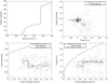 |
Fig. 4 Top-left panel: number of family core members found as a function of velocity cutoff, using the HCM. The second jump in the number of linked asteroids, at 460 m s−1, is our adopted value of velocity cutoff. Other panels: distribution of the X-complex asteroid with 0.1 < pV < 0.3 of the inner main belt in the three proper elements a, e, sin i. The cluster (of grey points) centred at (a, e, sin i) ~ (2.28, 0.144, 0.095 au) is the core of the Baptistina asteroid family. |
 (4)
(4)
For each bin in e (and sin i), we count all bodies in a narrow sliver inside of the nominal V shape, that is, with (a, 1∕D) verifying the condition K|a − ac|≤ 1∕D ≤ K|a − ac| + W (where W is small fraction, e.g. 10–20%, of the value of K) and whose values of e (and sin i) are included in each bin. We then multiply the number of asteroids in each bin by the value of e (and sin i) of the centre of the bin and divide by the bin area. The number obtained for each bin is normalised by the total number of asteroids multiplied by the total area. The multiplication by the value of e and sin i for the eccentricity and the inclination histograms, respectively, is due to the fact that the orbital phase space available to asteroids is proportionalto e and sin i.
If the histograms of the normalised e and sin i distributions have well-defined peaks (see Fig. A.2) – which was not the case for the primordial asteroid family discovered by Delbo et al. (2017) – we denote the coordinates of the peak in eccentricity and inclination as ec and ic, respectively.
Subsequently, we use the Hierarchical Clustering Method (HCM; Zappalà et al. 1990) to determine the population that clusters around the family centre. To do so, we create a fictitious asteroid with orbital elements (ac, ec, ic) that we use as central body for the HCM algorithm. We use the HCM version of Nesvorný et al. (2015). We follow this procedure to avoid using real asteroids near the vertex of the family V shape. This is because for old and primordial families, it is possible that the parent asteroid was lost due to the dynamical evolution of the main belt (Delbo et al. 2017; Minton & Malhotra 2010).
The HCM algorithm relies on the “standard metric” of Zappalà et al. (1990, 1995) to calculate a velocity difference between two asteroid orbits. It then connects bodies falling within a cut-off velocity (Vc), creating clusters of asteroids as a function of Vc. The number of asteroids in the cluster Nc is a monotonic growing function of Vc, but as this latter increases the number of family members can grow with steps. For small cut-off velocities no asteroids are linked; when Vc reaches a value appropriate to cluster members of the family, the number of members jumps up, followed by a steady increase of Nc with a further increasing value of Vc, until all family members are linked to each other; if one were to continue increasing Vc, the value of Nc would jump up again followed by another slow increase. This second jump indicates the limit of the family, because after the jump, the HCM accretes objects outside the family or asteroids belonging to adjacent families. We use the value Vc at the second jump of Nc to define the family. More precisely, we run the HCM for values of Vc between 10 and 600 m s−1 with a step of 1 m s−1 and we take the minimum value of this parameter to be the nominal Vc of the family, allowing us to link the largest number of asteroids before the second jump in the value of Nc.
4.5 Family age determination
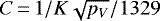
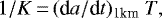
In order to provide an estimate for the age of the family T, and its uncertainty, we use two methods. Firstly, we follow the procedure of Delbo et al. (2017), which is based on the methods of Spoto et al. (2015) that gives an approximate age for the family (as this technique does not take into account the effect of YORP cycles on the Yarkovsky drift of asteroids). The age (T) and its uncertainty are derived from the inverse slope of the V shape given by Eq. (5):
 (5)
(5)
where (da/dt)1km is the rate ofchange of the orbital proper semi-major axis with time (t) for an asteroid of 1 km in size due to the Yarkovsky effect (Bottke et al. 2006). We perform 106 Monte Carlo simulations, where at each iteration, random numbers are obtained from the probability distributions of K and (da/dt)1km in order to be used in Eq. (5). The (da/dt)1km value, obtained by applying the formulas of Bottke et al. (2006), is calculated at each Monte Carlo iteration, and depends on asteroid properties such as the heliocentric distance, infrared emissivity, bolometric Bond albedo (A), thermal inertia, bulk density, rotation period, and obliquity (γ), which is the angle between the spin vector of an asteroid and its orbital plane. The border of the V shape is determined by those asteroids drifting with maximum |da∕dt|∝ cosγ, meaning that we assume γ = ± 90°. For the other parameters, we extract random numbers from their probability distributions. The calculation of the probability distribution for each of the relevant parameters is described in Sect. 5. A change in the luminosity of the Sun as a function of time is taken into account using Eq. (4) of Carruba et al. (2015).
5 Results
We use the V-shape-searching technique on all moderate-albedo X-types of the inner main belt selected as detailed in Sect. 4.1. The result of the V shape search is shown in Fig. 3, where we identify a prominent peak of  at ac = 2.38 au and K = 1.72 km−1 au−1, which we identify with the label “1” in the figure. A further two peaks of
  at ac ~ 2.28 au and K ~1 km−1 au−1 (peak “2” of Fig. 3) and at ac = 2.26 au and K = 11.9 km−1 au−1 are also visible. The latter peak corresponds to the V shape of the Baptistina asteroid family (Nesvorný et al. 2015; Bottke et al. 2007; Masiero et al. 2012b), while the first and second peaks represent previously unknown V shapes (Fig. A.1 gives a graphical representation of the V shapes).
We begin focusing on the V shape centred at ac = 2.38. In order to determine the uncertainties on the values of its ac and K parameters, we perform a Monte Carlo simulation as described in Sect. 4.2 (the ranges of parameter values explored is 1 ≤ K ≤ 4 au−1 km−1 and 2.34 ≤ ac ≤ 2.40 au). We find that the uncertainties on the determination of ac and K are 0.006 au and 0.1 au−1 km−1, respectively. We note that the average catalogue albedo uncertainty for our pool of asteroids is about 30% relative value, which is similar to the albedo uncertainty estimated by Pravec et al. (2012) for the WISE catalogue.
Subsequently, we study the inclination and eccentricity distributions of those asteroids inside and near the border of the V shape centred at (ac, K) = (2.38 au, 1.72 km−1 au−1), as detailed in Sect. 4.2. These distributions, presented in Fig. A.2, show maxima at ec = 0.12 and sin (ic) = 0.14, indicating a potential clustering ofobjects in (e, i) space. Together with the vertex of the V shape, this information points to a putative centre of the family at (ac, ec, sin ic) = (2.38, 0.12, 0.14 au). We assume a fictitious asteroid with the above-mentioned proper orbital elements for the central body for the HCM algorithm. The latter is used to link asteroids as a function of Vc. Again, we use moderate albedo X-type asteroids of the inner main belt selected as described in Sect. 4.1, as input population for the HCM. The number of asteroids linked by the HCM is displayed in Fig. 4, which shows that Vc ~ 460 s−1 identifies the second jump in the number of bodies linked to the family as a function of Vc. We thus take this value as the nominal Vc for this cluster. The lowest-numbered and largest asteroid of this cluster is the M-type (161) Athor, which is also the asteroid closest to the vertex of the V shape.
Figure 4 shows that X-type asteroids of the inner main belt have bimodal distributions in e and sin i with the cluster identified by the HCM and parented by (161) Athor located at high inclination (sin i > 0.1), and low eccentricity (e ~ 0.1). Another very diffused group of asteroids appears at low inclination and high eccentricity (sin i < 0.1, e > 0.12). Once members of the Baptistina family are removed, most X-type asteroids with sin i < 0.1 and e > 0.12 are included inside the V shape defined by (ac, K) = (2.38 au, 1.72 km−1 au−1), which also borders the HCM cluster of Athor. We make the hypothesis that the group associated to (161) Athor by the HCM is the core of a collisional family and the other asteroids that are within the V shape and have (sin i < 0.1 and e > 0.12) form the family “halo” (Parker et al. 2008; Brož & Morbidelli 2013) of the Athor family.
A fundamental test that these two groups of asteroids are members of the same collisional family, dispersed by the Yarkovsky effect, comes from rejecting the null hypothesis that the asteroids semimajor axis could be derived from size-independent distributions. We therefore performed the statistical test described in Sect. 4.3 and find no cases in 106 trials where we can generate a V shape like that observed by drawing randomly from the semimajor distribution of all X-type asteroids of the IMB. This demonstrates that the V shape is not just a consequence of the statistical sampling of an underlying size-independent distribution, but is a dispersion of asteroids from a common origin due to the Yarkovsky effect, which is a strong indication that they belong to a collisional family. We use 146 observed bodies, 5 of which are outside the borders of the V shape. The average number of simulated bodies that fall outside the V shape is 23 with a standard deviation of 3.5.
In order to determine the age of the Athor family, as described in Sect. 4.5, we need to estimate the drift rate due to the Yarkovsky effect, which depends on a number of parameters such as heliocentric distance, bulk density, rotation period, and thermal inertia. We fix the semimajor axis at the centre of the family (ac = 2.38 au), and we determine the probability distribution for the albedo, rotational period, density, and thermal inertia, which are all the parameters relevant to estimate the value of da/dt in Eq. (5). Values of the bolometric Bond’s albedo (A) are obtained from those of the geometric visible albedo pV via the equation A = pV(0.29 + 0.684G), where pV and G are given in Table B.1. It is possible to demonstrate that the distribution of A is well approximated by a Gaussian function centred at A = 0.073 and with σ = 0.02. Density has not been calculated for any of the family members. We therefore estimate this parameter by taking a weighted mean density of asteroids belonging to the X complex and with 0.1 ≤ pV ≤ 0.3 (see Table B.4). The weights are given by the inverse square of density uncertainties. We find an average value of 3500 kg m−3 and an uncertainty of the mean of 150 kg m−3. We estimate that a value three times larger, that is, 450 kg m−3, is more appropriate for the density uncertainty. For the age determination, we therefore assume that the probability function of the density of family members is a Gaussian function centred at 3500 kg m−3 and with σ = 450 kg m−3. The asteroid (757) Portlandia, with a spherical equivalent diameter of about 33 km, is at the moment of writing the only family member with known thermal inertia value (Γ) around 60 J m−2 s−0.5 K−1 (Hanuš et al. 2018). The other non-family X-complex asteroids with 0.1 < pV < 0.3 with measured thermal inertia values are (272) Antonia, (413) Edburga, (731) Sorga, (789) Lena, (857) Glasenappia, and (1013) Tombecka with values of 75, 110, 62, 47, 47, and 55 J m−2 s−0.5 K−1, respectively, which were measured at heliocentric distances (rh) of 2.9, 2.9, 3.3, 2.7,2.3, and 3.1 au, respectively (Hanuš et al. 2018). Since thermal inertia is temperature dependent (Rozitis et al. 2018) and the surface temperature of an asteroid is a function of its heliocentric distance, we correct these thermal inertia values to 2.38 au assuming that  (Delbo et al. 2015). We find a mean value of 80 J m−2 s−0.5 K−1 and a standard deviation of 25 J m−2 s−0.5 K−1. We therefore assume a Gaussian with these parameters for the thermal inertia probability distribution of the family members. We assume the rotation period of family members to be represented by a uniform distribution with values between 2.41 and 6.58 h. This is because the twelve family members with known rotational periods, (757) Portlandia, (2419) Moldavia, (4353) Onizaki, (5236) Yoko, and (7116) Mentall, are very close to the inward border of the family V shape, and are therefore the best candidates to use for the calculation of da/dt due to the Yarkovsky effect. As in the case of the primordial family of Delbo et al. (2017) we find here that the Monte Carlo simulations produce an almost lognormal probability distribution of the ages of the family. The best Gaussian fit to this distribution in logT-space allows us toestimate the most likely age of the family, and its formal standard deviations, to be 3.0
 Gyr.
Gyr.
Now, we turn our attention to the “background”, that is, those asteroids of the X-type population of the inner main belt with 0.1 < pV < 0.3 which remain after we remove the members of the core and halo of the Athor family and the members of the Baptistina family: Fig. 5 shows that their (a, 1∕D) distribution appears to have a border that follows the outward slope of the V shape with parameters ac ~ 2.28 au and K ~ 1 km−1 au−1, which corresponds to the peak labelled “2” in Fig. 3.
In order to determine the uncertainties on the values of its ac and K parameters, we perform a Monte Carlo simulation as described in Sect. 4.2, where the ranges of parameter values explored are 0.0 ≤ K ≤ 2 au−1 km−1 and 2.22 ≤ ac ≤ 2.32 au. We find that the uncertainties on the determination of ac and K are 0.02 au and 0.2 au−1 km−1, respectively.
We perform the statistical test described in Sect. 4.3 and find about 2870 cases in 106 trials where we can generate a V shape such as the one observed from a size-independent semi-major axis distribution of asteroids. This demonstrates that this V shape is also probably not just a consequence of the statistical sampling of an underlying size-independent semimajor axis distribution, however with smaller statistical significance than the V shape of Athor and the V shape of the primordial family of Delbo et al. (2017). We use 183 observed bodies, none of which are outside the borders of the V shape (all the grey points of Fig. 5). The average number of simulated bodies that fall outside the V shape is 4.8 with a standard deviation of 1.8. This means that it is possible that this second V shape is simply due to statistical sampling, despite this probability being very low (~0.29%, which means that this family is robust at 2.98σ). Assuming similar physical properties to those described above, the age ratio between this second V shape and the one centred on (161) Athor is given, to first order, by the ratio of the V-shape slopes, that is, approximately 5.16 Gyr. We refine the age using the same aforementioned Monte Carlo method (taking into account the change of the solar constant with time), and find that the distribution of the family age (t0) values is well represented by a Gaussian function in log10(t0) centred at 0.7 and with a standard deviation of 0.1. This corresponds to a family age of 5.0 Gyr. Given the errors involved in the age estimation process, we conclude that this V shape could be as old as our solar system.
The lowest-numbered asteroid of this V shape is the asteroid (689) Zita with a diameter of 15.6 km, while the largest-numbered member of this family is the asteroid (1063) Aquilegia, which has a diameter of 19 km. We highlight that the CX classification of Zita comes from multi-filter photometry of Tholen & Barucci (1989), and its pV = 0.10 ± 0.02 is also compatible with an object of the C complex.
6 Discussion
First of all, we advocate caution when dealing with the parenthood of the families, because it is possible that neither (161) Athor nor (689) Zita are the parents of their respective families. This is due to the fact that these families are several gigayears old and have likely lost a significant fraction of their members by collisional and dynamical depletion possibly including their parent bodies or largest remnants (as described by Delbo et al. 2017, and references therein). This is particularly important for the Zita family, which we argue predated the giant planet instability, and to a lesser extent for the Athor family. Some of the Zita family members have sizes of a few kilometres. The lifetime of these bodies in the main belt, before they breakup by collisions, is smaller than the age of the family (Bottke et al. 2005). It is therefore likely that they were created by the fragmentation of a larger Zita family member due to a collision that was more recent than the family-forming one. Fragmentation of bodies inside a family produces new asteroids whose coordinates in the (a, 1∕D) space still lie inside the family V shape.
Thirteen members of the Athor family have visible spectra from the literature, which we plot in Fig. A.3. Of these, the asteroid (4353) Onizaki has dubious classification and could be a low-albedo S-type (Bus & Binzel 2002), and thus an interloper to this family. The remaining objects have spectra similar to the Xc or the Xk average spectra (Fig. A.3). No family member has near-infrared spectroscopy. Further spectroscopic surveys of members of the Athor family will better constrain the composition of this family (Avdellidou et al., in prep.). In addition, the currently on-going space mission Gaia is collecting low-resolution spectra of asteroids in the visible (Delbo et al. 2012); the Gaia Data Release 3 in 2021, will contain asteroid spectra and should help to further constrain family membership.
Fourteen core members of the Athor family – asteroids numbered 2419, 11977, 12425, 17710, 21612, 30141, 30814, 33514, 34545, 42432, 43739, 54169, 68996, and 80599 – and seven members of the halo of Athor family – 1697, 2346, 3865, 8069, 29750, 42016, and 79780 – were also linked by Nesvorný et al. (2015) to the family of the asteroid (4) Vesta. None of these asteroids are classified as V-type, which is expected given the composition of (4) Vesta and its family. The geometric visible albedo distribution of these asteroids has a mean value of 0.18 and standard deviation of 0.04, while that of the Vesta family has a mean value of 0.35 and standard deviation of 0.11. The albedo values and spectra or spectrophotometric data of these asteroids are therefore incompatible with those of the Vesta family, making them very likely interlopers that are linked to (4) Vesta by the HCM because of their orbital element proximity. While the V-shape family identification is quite robust against interlopers, in particular because we apply it on compositionally similar asteroids, the presence of interlopers is still possible. In our case, interlopers are mostly the result of uncertainties in the albedo and spectral identification. We estimated the effect of albedo uncertainty on the selection of asteroids following the Monte Carlo method described in Sect. 4.2. We find that the number of asteroids selected by the criterion 0.1 ≤ pV ≤ 0.3 varies within 6%. Uncertainty in spectral class assignation probably adds another 5–10% to the number of interlopers.
In Fig. 4 one can locate the core of the ν6 secular resonance at ~2.15 au for sin i ~ 0.1 and Fig. 5 shows that the inward border of the V shape of the Athor family crosses a = 2.15 au for 1∕D ~ 0.4 km−1. This implies that the Athor family could feed the ν6 with asteroids with D = 2.5 km or smaller. However, members of the Athor family already start to be removed from the main belt at a ~ 2.2 au due to the width of the dynamically unstable region around the ν6. This indicates that Athor family members with sizes D ≲ 2.5–3 km can leave the main belt and become NEAs. Another possible escape route from the main belt to near-Earth space is the zone of overlapping J7:2 and M5:9 MMR with Jupiter and Mars, respectively (which is also an important escape route for the Baptistina family members; Bottke et al. 2007). Asteroids drifting with d a∕dt < 0 from the centre of the Athor family at a = 2.38 au would encounter the overlapping J7:2 and M5:9 MMR before the ν6. Indeed, the number density of Athor family members visually appears to decrease inward (to the left) of the overlapping J7:2 and M5:9 (Fig. 5). Twelve of the fifteen X-complex NEAs with moderate geometric visible albedo (0.1 < pV < 0.3) have osculating sin i > 0.1, indicating their likely origin from the moderate inclination part of the inner main belt, which is also the location of the Athor family.
Using the aforementioned argument, one can see that the Zita family can deliver asteroids with 1∕D ≳ 0.12 km−1, that is, D ≲ 8.3 km, to the ν6 resonance. Visual inspection of Fig. 5 suggests that the number density of Zita family members firstly increases and then rapidly decreases for a < 2.2545 au, where the J7:2 and M5:9 resonances are overlapping. The number density increase is confined within the inward section (i.e. to the left side) of the V shape of the Baptistina family (Fig. 5) despite these asteroids not being linkedby Nesvorný et al. (2015) to this family. Out of the 47 asteroids that in Fig. 5 reside between the inward border of the Baptistina family and the J7:2|M5:9 resonances (i.e. those that have 1∕D ≤ 11.9 × (a − 2.26) km−1 and a < 2.2545 au), 27 are linked to the Flora asteroid family by Nesvorný et al. (2015). We suspect that these asteroids could in reality be Babptistina family members, although they are currently linked to the Flora family by the HCM of Nesvorný et al. (2015). As in the case of the Athor family, members of the Zita family drifting with d a∕dt < 0 from the centre of the Athor family at a = 2.28 au would encounter the overlapping J7:2 and M5:9 MMRs before the ν6. Both Athor and Zita families can also deliver asteroids of D ≲ 5 km to the near-Earth space via the 3:1 MMR with Jupiter.
While the e and i distributions of the ~3 Gyr-old Athor family are still relatively compact, this is not the case for the Zita family. The e and i distributions of the latter family resemble those calculated by Brasil et al. (2016) during the dynamical dispersal of asteroids – without scattering caused by close encounters with a fifth giant planet – due to the giant planet instability (Tsiganis et al. 2005; Morbidelli et al. 2015). Together with its old age (> 4 Gyr) we interpret the large dispersion in e and i, covering thewhole phase space of the inner main belt, as a sign that the Zita family is primordial, that is, it formed before the giant planetinstability. This instability is needed to explain the orbital structure of the transneptunian objects (Levison et al. 2008; Nesvorný 2018), the capture of the Jupiter trojans from objects scattered inward from the primordial transneptunian disc (Morbidelli et al. 2005; Nesvorný et al. 2013), the orbital architecture of the asteroid belt (Roig & Nesvorný 2015), and that of the irregular satellites of the giant planets (Nesvorný et al. 2007); see Nesvorný (2018) for a review. The exact timing of this event is still debatable and is a matter of current research: it was initially tiedto the Late Heavy bombardment and the formation of the youngest lunar basins, i.e. several hundreds (~700) million years after the formation of the calcium- and aluminium-rich inclusions (Bouvier & Wadhwa 2010; Amelin et al. 2002), which is taken as the reference epoch for the beginning of our solar system. However, recent works tend to invoke an earlier instability (Morbidelli et al. 2018). In addition, simulations by Nesvorný et al. (2018) of the survival of the binary Jupiter Trojan Patroclus–Menoetius, which was originally embedded in a massive transneptunian disc, but dislodged from this and captured as trojan by Jupiter during the instability, indicate that this disc had to be dispersed within less than 100 Myr after the beginning of the solar system. Since the dispersion of the transneptunian disc is a consequence of the giant planet instability (Levison et al. 2008), one can derive the upper limit of 100 Myr for the time for this event (Nesvorný et al. 2018). Moreover, Clement et al. (2018) propose that the instability occurred only a few (1–10) million years after the dispersal of the gas of the protoplantery disc. The age estimate of the Zita family, given its uncertainty, can only constrain the epoch of the giant instability to be ≲600 Myr after the beginning of the solar system. The major source of uncertainty is the determination of the value of d a∕dt due to the Yarkovsky effect for family members. It is expected that end-of-mission Gaia data will allow the Yarkosvky d a∕dt to be constrained for main-belt asteroids (Gaia Collaboration 2018).
Following the logic of Delbo et al. (2017), we propose that X-complex asteroids with geometric visible albedo between 0.1 and 0.3 of the inner part of the main belt have two populations of bodies: one that comprises the bodies inside V shapes (Athor, Baptistina, and Zita), but not the parent bodies of the families, and another that includes only those nine bodies that are outside V shapes and the parent bodies of the families: (161) Athor, (298) Baptistina, and (689) Zita. Objects of the former population are family members and were therefore created as fragments of parent asteroids that broke up during catastrophic collisions. On the other hand, asteroids from the latter population cannot be created from the fragmentation of the parent body of a family and as such we consider that they formed as planetsimals by dust accretion in the protoplanetary disc. The implication is that the vast majority of the X-types with moderate albedo of the inner main belt are genetically related to a few parent bodies – Zita, Athor, Hertha (Dykhuis & Greenberg 2015), and possibly Baptistina (Bottke et al. 2007), even though the latter family could be composed by objects whose composition is similar to that of impact-blackened ordinary chondrite meteorites (Reddy et al. 2014) and is therefore more similar to S-type asteroids.
We plot the size distribution of the population of bodies that are not included in V shapes together with those already identified by Delbo et al. (2017) in Fig. 6. As progenitors of the Athor and Zita families, we also add two asteroids whose effective diameters are 133 and 130 km as deduced by the cubic root of the sum of the cube of the diameters of the members of the Athor (core and halo) and Zita families, respectively. These sizes represent a lower limit to the real sizes of the parents that broke up to form the families. Following the same procedure as Delbo et al. (2017) we compute an upper limit for the original size distribution of the planetesimals taking into account asteroid dynamical and collisional loss as a stochastic process. The resulting original size distribution (Fig. 6) is still shallower than predicted by some current accretion models Johansen et al. (2015); Simon et al. (2016), confirming the hypothesis that planetesimals were formed big Morbidelli et al. (2009); Bottke et al. (2005). Compared to previous results (Delbo et al. 2017), which could not find planetesimals smaller than 35 km in diameter, here we identify planetesimals with D < 35 km, but the slope of the size distribution of the planetesimals below this latter diameter is very similar to, and even shallower than, the previously computed upper bound (compare Fig. 6 with Figs. 4 and S7 of Delbo et al. 2017).
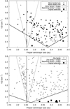 |
Fig. 5 Distribution of X-complex asteroids with 0.1 < pV < 0.3 of the inner main belt in the (a, 1∕D) space and that do not belong to the Baptistina asteroid family according to Nesvorný et al. (2015). Top panel: asteroids with sin i > 0.1 and e < 0.12. Objects represented by circles are Athor family members; the squares are planetesimals. Bottom panel: all the other asteroids that belong neither to Baptistina nor the core or halo of Athor. Those represented with circles are Zita family members. Squares are the planetesimals. The position of the overlapping J7:2 MMR and the M5:9 MMR is drawn with a vertical bar. The V shapes of the Hathor, Zita, and Baptistina families are plotted (but not the members of the Baptistina family). As discussed in Sect. 6, we define planetesimals as those asteroids that cannot be included into V shapes. |
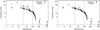 |
Fig. 6 Cumulative size distribution of planetesimals. This is the cumulative size distribution of those asteroids that are outsideV shapes and thus probably do not belong to a family. Additionally, in this dataset, are included the parent bodies of families, as originally they belonged to the planetesimal population. The distribution is then corrected for the maximum number of objects that were lost due the collisional and dynamical evolution; this gives an upper limit for the distribution of the planetesimals (open squares). Functions of the form N(> D) = N0Dβ, where N is the cumulative number of asteroids, are fitted piecewise in the size ranges D > 100, 35 < D < 100, and D < 35 km. For the original planetesimals size distribution, we obtain the values of β reported by the labels in the plot. Left panel: correction to the number of asteroids is calculated taking into account 10 Gyr of collisional evolution in the present main-belt environment, following the prescription of Bottke et al. (2005). Right panel: correction to the number of asteroids taking into account 4.5 Gyr of collisional evolution in the present main-belt environment. |
7 Conclusions
Using our Vshape search method (Bolin et al. 2017), we have identified two previously unknown asteroid families in the inner portion of the main belt. These families are found amongst the X-type asteroids with moderate geometric visible albedo (0.1 < pV < 0.3). One of them, the Athor family is found to be ~3 Gyr-old, whereas the second one could be as old as the solar system. The core of the Athor family can be found using the HCM and the distributions of the inclinations, and the eccentricity of the proper orbital elements of its members is relatively compact. On the other hand, in the case of the older family, the eccentricities and inclinations of its member are spread over the entire inner main belt. This isan indication that this family could be primordial, which means that it formed before the giant planet instability.
We show that the vast majority of X-type asteroids of the inner main belt can be included into asteroid families. These asteroids are therefore genetically related and were generated at different epochs from the catastrophic disruption of very few parent bodies. The X-type asteroids with moderate albedo that are not family members in the inner main belt are only nine in number (ten if we include 298 Baptistina). Following the logic of our previous work (Delbo et al. 2017), we conclude that these bodies were formed by direct accretion of the solids in the protoplanetary disc and are thus surviving planetesimals. We combine the planetesimals found in this work with those from our previous study (Delbo et al. 2017) to create a planetesimal size distribution for the inner main belt. After correcting the number of objects due to the size-dependent collisional and dynamical evolution of the main belt, we find that the distribution is steep for D > 100 km but it becomes shallower for D < 100 km indicating that D ~ 100 km was a preferential size for planetesimal formation.
Acknowledgements
The work of C.A. was supported by the French National Research Agency under the project “Investissements d’Avenir” UCAJEDI with the reference number ANR-15-IDEX-01. M.D. acknowledges support from the French National Program of Planetology (PNP). This work was also partially supported by the ANR ORIGINS (ANR-18-CE31-0014). Here we made use of asteroid physical properties data from https://mp3c.oca.eu/, Observatoire de la Côte d’Azur, whose database is also mirrored at https://www.cosmos.esa.int/web/astphys. We thank Bojan Novakovic for his thorough review.
Appendix A Supplementary figures
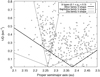 |
Fig. A.1 V shapes formed by the X-complex asteroids with geometric visible albedos in the range 0.1–0.3 of the inner main belt (2.1 < a < 2.5 au). |
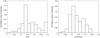 |
Fig. A.2 Distribution of the proper eccentricity and sinus of the proper inclination for X-type asteroids inside and near the border of the V shape with equation 1∕D = 1.72 |a − 2.38| km−1 (see text). The peaks show clustering of these asteroids, indicating the centre of the family. |
 |
Fig. A.3 Reflectance spectra from the literature of Athor family members numbered 161, 757, 1697, 1998, 2194 3007, 3665, 3704 3865, 4353, 4548, 4839, and 4845. The average reflectance spectra of the Xe, Xc, Xk, and C of the DeMeo et al. (2009) taxonomy (from http://smass.mit.edu/_documents/busdemeo-meanspectra.xlsx) are also plotted. References are: (161) from Bus & Binzel (2002), (757) from Bus & Binzel (2002), 1697 from Xu et al. (1995), (1998) from Bus & Binzel (2002), (2194) fromBus & Binzel (2002), (3007) from Bus & Binzel (2002), 3665 from Xu et al. (1995), (3704) from Bus & Binzel (2002), (3865) from Bus & Binzel (2002), (4353) from Bus & Binzel (2002), (4548) from Bus & Binzel (2002), (4839) from Bus & Binzel (2002), (4845) from Bus & Binzel (2002). |
Appendix B Supplementary tables
Athor family core members.
Athor family halo members.
Zita family members.
Known densities and their uncertainties of asteroids of the X complex and with 0.1 < pV < 0.3.
Original asteroids i.e. the surviving planetesimals.
References
- Alí-Lagoa, V., & Delbo, M. 2017, A&A, 603, A55 [NASA ADS] [CrossRef] [EDP Sciences] [Google Scholar]
- Amelin, Y., Krot, A. N., Hutcheon, I. D., & Ulyanov, A. A. 2002, Science, 297, 1678 [NASA ADS] [CrossRef] [PubMed] [Google Scholar]
- Avdellidou, C., Price, M. C., Delbo, M., Ioannidis, P., & Cole, M. J. 2016, MNRAS, 456, 2957 [NASA ADS] [CrossRef] [Google Scholar]
- Avdellidou, C., Price, M. C., Delbo, M., & Cole, M. J. 2017, MNRAS, 464, 734 [NASA ADS] [CrossRef] [Google Scholar]
- Avdellidou, C., Delbo, M., & Fienga, A. 2018, MNRAS, 475, 3419 [NASA ADS] [CrossRef] [Google Scholar]
- Basilevsky, A. T., Head, J. W., Horz, F., & Ramsley, K. 2015, Planet. Space Sci., 117, 312 [NASA ADS] [CrossRef] [Google Scholar]
- Binzel, R. P., Reddy, V., & Dunn, T. L. 2015, in Asteroids IV, eds. P. Michel (Tucson: University of Arizona Press), 243 [Google Scholar]
- Bolin, B. T., Delbo, M., Morbidelli, A., & Walsh, K. J. 2017, Icarus, 282, 290 [NASA ADS] [CrossRef] [Google Scholar]
- Bottke, W. F., Morbidelli, A., Jedicke, R., et al. 2002, Icarus, 156, 399 [NASA ADS] [CrossRef] [Google Scholar]
- Bottke, W. F., Durda, D. D., Nesvorný, D., et al. 2005, Icarus, 175, 111 [NASA ADS] [CrossRef] [Google Scholar]
- Bottke, W. F. J., Vokrouhlický, D., Rubincam, D. P., & Nesvorný, D. 2006, Ann. Rev. Earth Planet. Sci., 34, 157 [Google Scholar]
- Bottke, W. F., Vokrouhlický, D., & Nesvorný, D. 2007, Nature, 449, 48 [NASA ADS] [CrossRef] [Google Scholar]
- Bottke, W. F., Brož, M., O’Brien, D. P., et al. 2015a, in Asteroids IV, eds. P. Michel (Tucson: University of Arizona Press), 701 [Google Scholar]
- Bottke, W. F., Vokrouhlický, D., Walsh, K. J., et al. 2015b, Icarus, 247, 191 [NASA ADS] [CrossRef] [Google Scholar]
- Bouvier, A., & Wadhwa, M. 2010, Nat. Geosci., 3, 637 [NASA ADS] [CrossRef] [Google Scholar]
- Brasil, P. I. O., Roig, F., Nesvorný, D., et al. 2016, Icarus, 266, 142 [NASA ADS] [CrossRef] [Google Scholar]
- Brož, M., & Morbidelli, A. 2013, Icarus, 223, 844 [NASA ADS] [CrossRef] [Google Scholar]
- Brož, M., Morbidelli, A., Bottke, W. F., et al. 2013, A&A, 551, A117 [NASA ADS] [CrossRef] [EDP Sciences] [Google Scholar]
- Bus, S. J., & Binzel, R. P. 2002, Icarus, 158, 106 [CrossRef] [Google Scholar]
- Campins, H., Morbidelli, A., Tsiganis, K., et al. 2010, ApJ, 721, L53 [NASA ADS] [CrossRef] [Google Scholar]
- Campins, H., de León, J., Morbidelli, A., et al. 2013, AJ, 146, 26 [NASA ADS] [CrossRef] [Google Scholar]
- Carruba, V., Domingos, R. C., Nesvorný, D., et al. 2013, MNRAS, 433, 2075 [NASA ADS] [CrossRef] [EDP Sciences] [Google Scholar]
- Carruba, V., Nesvorný, D., Aljbaae, S., & Huaman, M. E. 2015, MNRAS, 451, 244 [NASA ADS] [CrossRef] [Google Scholar]
- Carruba, V., Nesvorný, D., Aljbaae, S., Domingos, R. C., & Huaman, M. 2016, MNRAS, 458, 3731 [NASA ADS] [CrossRef] [Google Scholar]
- Carry, B. 2012, Planet. Space Sci., 73, 98 [NASA ADS] [CrossRef] [Google Scholar]
- Carvano, J. M., Hasselmann, P. H., Lazzaro, D., & Mothé-Diniz, T. 2010, A&A, 510, A43 [NASA ADS] [CrossRef] [EDP Sciences] [Google Scholar]
- Clement, M. S., Kaib, N. A., Raymond, S. N., & Walsh, K. J. 2018, Icarus, 311, 340 [NASA ADS] [CrossRef] [Google Scholar]
- Ćuk, M., Gladman, B. J., & Nesvorný, D. 2014, Icarus, 239, 154 [NASA ADS] [CrossRef] [Google Scholar]
- Delbo, M., Gayon-Markt, J., Busso, G., et al. 2012, Planet. Space Sci., 73, 86 [NASA ADS] [CrossRef] [Google Scholar]
- Delbo, M., Mueller, M., Emery, J. P., Rozitis, B., & Capria, M. T. 2015, in Asteroids IV, eds. P. Michel (Tucson: University of Arizona Press), 107 [Google Scholar]
- Delbo, M., Walsh, K., Bolin, B., Avdellidou, C., & Morbidelli, A. 2017, Science, 357, 1026 [NASA ADS] [CrossRef] [Google Scholar]
- de León, J., Campins, H., Tsiganis, K., Morbidelli, A., & Licandro, J. 2010, A&A, 513, A26 [NASA ADS] [CrossRef] [EDP Sciences] [Google Scholar]
- de León, J., Pinilla-Alonso, N., Delbo, M., et al. 2016, Icarus, 266, 57 [NASA ADS] [CrossRef] [Google Scholar]
- Delisle, J. B., & Laskar, J. 2012, A&A, 540, A118 [NASA ADS] [CrossRef] [EDP Sciences] [Google Scholar]
- DeMeo, F. E.,& Carry, B. 2013, Icarus, 226, 723 [NASA ADS] [CrossRef] [Google Scholar]
- DeMeo, F. E., Binzel, R. P., Slivan, S. M., & Bus, S. J. 2009, Icarus, 202, 160 [NASA ADS] [CrossRef] [Google Scholar]
- DeMeo, F. E., Alexander, C. M. O., Walsh, K. J., Chapman, C. R., & Binzel, R. P. 2015, in Asteroids IV, eds. P. Michel, (Tucson: University of Arizona Press), 13 [Google Scholar]
- Dermott, S. F., Christou, A. A., Li, D., Kehoe, T. J. J., & Robinson, J. M. 2018, Nat. Astron., 2, 549 [NASA ADS] [CrossRef] [Google Scholar]
- Dykhuis, M. J., & Greenberg, R. 2015, Icarus, 252, 199 [NASA ADS] [CrossRef] [Google Scholar]
- Fornasier, S., Migliorini, A., Dotto, E., & Barucci, M. A. 2008, Icarus, 196, 119 [NASA ADS] [CrossRef] [Google Scholar]
- Fornasier, S., Clark, B. E., & Dotto, E. 2011, Icarus, 214, 131 [NASA ADS] [CrossRef] [Google Scholar]
- Fornasier, S., Lantz, C., Perna, D., et al. 2016, Icarus, 269, 1 [NASA ADS] [CrossRef] [Google Scholar]
- Fox, K., Williams, I. P., & Hughes, D. W. 1984, MNRAS, 208, 11P [NASA ADS] [CrossRef] [Google Scholar]
- Gaffey, M. J., Reed, K. L., & Kelley, M. S. 1992, Icarus, 100, 95 [NASA ADS] [CrossRef] [Google Scholar]
- Gaia Collaboration (Spoto, F., et al.) 2018, A&A, 616, A13 [NASA ADS] [CrossRef] [EDP Sciences] [Google Scholar]
- Granvik, M., Morbidelli, A., Jedicke, R., et al. 2016, Nature, 530, 303 [Google Scholar]
- Granvik, M., Morbidelli, A., Vokrouhlický, D., et al. 2017, A&A, 598, A52 [NASA ADS] [CrossRef] [EDP Sciences] [Google Scholar]
- Greenstreet, S., Ngo, H., & Gladman, B. 2012, Icarus, 217, 355 [NASA ADS] [CrossRef] [Google Scholar]
- Gustafson, B. A. S. 1989, A&A, 225, 533 [NASA ADS] [Google Scholar]
- Hanuš, J., Viikinkoski, M., Marchis, F., et al. 2017, A&A, 601, A114 [NASA ADS] [CrossRef] [EDP Sciences] [Google Scholar]
- Hanuš, J., Delbo, M., Durech, J., & Alí-Lagoa, V. 2018, Icarus, 309, 297 [NASA ADS] [CrossRef] [Google Scholar]
- Hardersen, P. S., Gaffey, M. J., & Abell, P. A. 2005, Icarus, 175, 141 [NASA ADS] [CrossRef] [Google Scholar]
- Hörz, F., & Cintala, M. 1997, Meteor. Planet. Sci., 32, 179 [NASA ADS] [CrossRef] [Google Scholar]
- Jewitt, D., Weaver, H., Mutchler, M., Larson, S., & Agarwal, J. 2011, ApJ, 733, L4 [NASA ADS] [CrossRef] [Google Scholar]
- Johansen, A., Mac Low, M.-M., Lacerda, P., & Bizzarro, M. 2015, Sci. Adv., 1, 1500109 [NASA ADS] [CrossRef] [Google Scholar]
- Lauretta, D. S., Barucci, M. A., Bierhaus, E. B., et al. 2012, Asteroids, Comets, Meteors, No. 229, 2005, eds. D. Lazzaro, S. Ferraz-Mello, & J.A. Fernandez, Proc. IAU Symp., 1667, 6291 [Google Scholar]
- Lazzaro, D., Angeli, C. A., Carvano, J. M., et al. 2004, Icarus, 172, 179 [CrossRef] [Google Scholar]
- Levison, H. F., Morbidelli, A., Van Laerhoven, C., Gomes, R., & Tsiganis, K. 2008, Icarus, 196, 258 [NASA ADS] [CrossRef] [Google Scholar]
- Lucas, M. P., Emery, J. P., Pinilla-Alonso, N., Lindsay, S. S., & Lorenzi, V. 2017, Icarus, 291, 268 [NASA ADS] [CrossRef] [Google Scholar]
- Mainzer, A., Bauer, J., Grav, T., et al. 2014, ApJ, 784, 110 [NASA ADS] [CrossRef] [Google Scholar]
- Masiero, J. R., Mainzer, A. K., Grav, T., et al. 2011, ApJ, 741, 68 [NASA ADS] [CrossRef] [Google Scholar]
- Masiero, J. R., Mainzer, A. K., Grav, T., et al. 2012a, ApJ, 759, L8 [NASA ADS] [CrossRef] [Google Scholar]
- Masiero, J. R., Mainzer, A. K., Grav, T., Bauer, J. M., & Jedicke, R. 2012b, ApJ, 759, 14 [NASA ADS] [CrossRef] [Google Scholar]
- Masiero, J. R., Grav, T., Mainzer, A. K., et al. 2014, ApJ, 791, 121 [NASA ADS] [CrossRef] [Google Scholar]
- McCord, T. B., Li, J. Y., Combe, J. P., et al. 2012, Nature, 491, 83 [NASA ADS] [CrossRef] [Google Scholar]
- Milani, A., Cellino, A., Knežević, Z., et al. 2014, Icarus, 239, 46 [NASA ADS] [CrossRef] [Google Scholar]
- Milani, A., Knežević, Z., Spoto, F., et al. 2017, Icarus, 288, 240 [NASA ADS] [CrossRef] [Google Scholar]
- Milić Žitnik, I., & Novaković, B. 2016, ApJ, 816, L31 [NASA ADS] [CrossRef] [Google Scholar]
- Minton, D. A., & Malhotra, R. 2010, Icarus, 207, 744 [NASA ADS] [CrossRef] [Google Scholar]
- Morate, D., de León, J., De Prá, M., et al. 2016, A&A, 586, A129 [NASA ADS] [CrossRef] [EDP Sciences] [Google Scholar]
- Morbidelli, A., & Henrard, J. 1991, Celest. Mech. Dyn. Astron., 51, 131 [NASA ADS] [CrossRef] [Google Scholar]
- Morbidelli, A., & Vokrouhlický, D. 2003, Icarus, 163, 120 [NASA ADS] [CrossRef] [Google Scholar]
- Morbidelli, A., Levison, H. F., Tsiganis, K., & Gomes, R. 2005, Nature, 435, 462 [NASA ADS] [CrossRef] [PubMed] [Google Scholar]
- Morbidelli, A., Bottke, W. F., Nesvorný, D., & Levison, H. F. 2009, Icarus, 204, 558 [NASA ADS] [CrossRef] [Google Scholar]
- Morbidelli, A., Walsh, K. J., O’Brien, D. P., Minton, D. A., & Bottke, W. F. 2015, in Asteroids IV eds. P. Michel (Tucson: University of Arizona Press), 493 [Google Scholar]
- Morbidelli, A., Nesvorný, D., Laurenz, V., et al. 2018, Icarus, 305, 262 [NASA ADS] [CrossRef] [Google Scholar]
- Neese, C. 2010, Asteroid Taxonomy V6.0. EAR-A-5-DDR-TAXONOMY-V6.0. NASA Planetary Data System [Google Scholar]
- Nesvorný, D. 2018, ARA&A, 56, 137 [NASA ADS] [CrossRef] [Google Scholar]
- Nesvorný, D., Vokrouhlický, D., & Morbidelli, A. 2007, AJ, 133, 1962 [NASA ADS] [CrossRef] [Google Scholar]
- Nesvorný, D., Vokrouhlický, D., & Morbidelli, A. 2013, ApJ, 768, 45 [NASA ADS] [CrossRef] [Google Scholar]
- Nesvorný, D., Brož, M., & Carruba, V. 2015, in Asteroids IV, eds. P. Michel, (Tucson: University of Arizona Press), 297 [Google Scholar]
- Nesvorný, D., Vokrouhlický, D., Bottke, W. F., & Levison, H. F. 2018, Nat. Astron., 130, 2392 [Google Scholar]
- Nugent, C. R., Mainzer, A., Masiero, J., et al. 2015, ApJ, 814, 117 [NASA ADS] [CrossRef] [Google Scholar]
- Nugent, C. R., Mainzer, A., Bauer, J., et al. 2016, AJ, 152, 63 [NASA ADS] [CrossRef] [Google Scholar]
- Parker, A., Ivezić, Ž., Jurić, M., et al. 2008, Icarus, 198, 138 [NASA ADS] [CrossRef] [Google Scholar]
- Popescu, M., Licandro, J., Carvano, J. M., et al. 2018, A&A, 617, A12 [NASA ADS] [CrossRef] [EDP Sciences] [Google Scholar]
- Pravec, P., Harris, A. W., Kusnirak, P., Galád, A., & Hornoch, K. 2012, Icarus, 221, 365 [NASA ADS] [CrossRef] [Google Scholar]
- Reddy, V., Sanchez, J. A., Bottke, W. F., et al. 2014, Icarus, 237, 116 [NASA ADS] [CrossRef] [Google Scholar]
- Roig, F., & Nesvorný, D. 2015, AJ, 150, 186 [NASA ADS] [CrossRef] [Google Scholar]
- Rozitis, B., Green, S. F., MacLennan, E., & Emery, J. P. 2018, MNRAS, 477, 1782 [NASA ADS] [CrossRef] [Google Scholar]
- Ryan, E. L., & Woodward, C. E. 2010, AJ, 140, 933 [NASA ADS] [CrossRef] [Google Scholar]
- Sierks, H., Lamy, P., Barbieri, C., et al. 2011, Science, 334, 487 [NASA ADS] [CrossRef] [Google Scholar]
- Simon, J. B., Armitage, P. J., Li, R., & Youdin, A. N. 2016, ApJ, 822, 55 [NASA ADS] [CrossRef] [Google Scholar]
- Spoto, F., Milani, A., & Knežević Z. 2015, Icarus, 257, 275 [NASA ADS] [CrossRef] [Google Scholar]
- Tedesco, E. F., Noah, P. V., Noah, M., & Price, S. D. 2002, AJ, 123, 1056 [Google Scholar]
- Tholen, D. J.,& Barucci, M. A. 1989, in Asteroids II, eds. R.P. Binzel, T. Gehrels, & M.S. Matthews (Tucson: The University of Arizona Press), 298 [Google Scholar]
- Todorović, N. 2018, MNRAS, 475, 601 [NASA ADS] [Google Scholar]
- Tsiganis, K., Gomes, R., Morbidelli, A., & Levison, H. F. 2005, Nature, 435, 459 [NASA ADS] [CrossRef] [PubMed] [Google Scholar]
- Tsirvoulis, G., Morbidelli, A., Delbo, M., & Tsiganis, K. 2018, Icarus, 304, 14 [NASA ADS] [CrossRef] [Google Scholar]
- Turrini, D., Svetsov, V., Consolmagno, G., Sirono, S., & Pirani, S. 2016, Icarus, 280, 328 [NASA ADS] [CrossRef] [Google Scholar]
- Usui, F., Kuroda, D., Müller, T. G., et al. 2011, PASJ, 63, 1117 [NASA ADS] [CrossRef] [Google Scholar]
- Vernazza, P., Binzel, R. P., Thomas, C. A., et al. 2008, Nature, 454, 858 [NASA ADS] [CrossRef] [Google Scholar]
- Vernazza, P., Binzel, R. P., Rossi, A., Fulchignoni, M., & Birlan, M. 2009, Nature, 458, 993 [NASA ADS] [CrossRef] [Google Scholar]
- Vernazza, P., Castillo-Rogez, J., Beck, P., et al. 2017, AJ, 153, 72 [NASA ADS] [CrossRef] [Google Scholar]
- Vokrouhlický, D., Brož, M., Bottke, W. F., Nesvorný, D., & Morbidelli, A. 2006, Icarus, 182, 118 [NASA ADS] [CrossRef] [Google Scholar]
- Vokrouhlický, D., Bottke, W. F., & Nesvorný, D. 2017, AJ, 153, 172 [NASA ADS] [CrossRef] [Google Scholar]
- Walsh, K. J., Delbo, M., Bottke, W. F., Vokrouhlický, D., & Lauretta, D. S. 2013, Icarus, 225, 283 [NASA ADS] [CrossRef] [Google Scholar]
- Warner, B., Harris, Alan, W., & Pravec, P. 2009, Icarus, 202, 134 [NASA ADS] [CrossRef] [Google Scholar]
- Williams, I. P., & Wu, Z. 1993, MNRAS, 262, 231 [NASA ADS] [Google Scholar]
- Xu, S., Binzel,R. P., Burbine, T. H., & Bus, S. J. 1995, Icarus, 115, 1 [NASA ADS] [CrossRef] [Google Scholar]
- Zappala, V., Farinella, P., Knezevic, Z., & Paolicchi, P. 1984, Icarus, 59, 261 [NASA ADS] [CrossRef] [Google Scholar]
- Zappalà, V., Cellino, A., Farinella, P., & Knežević, Z. 1990, AJ, 100, 2030 [NASA ADS] [CrossRef] [Google Scholar]
- Zappalà, V., Bendjoya, P., Cellino, A., Farinella, P., & Froeschlé, C. 1995, Icarus, 116, 291 [NASA ADS] [CrossRef] [Google Scholar]
https://www.minorplanetcenter.net, downloaded Nov 2016.
All Tables
Known densities and their uncertainties of asteroids of the X complex and with 0.1 < pV < 0.3.
All Figures
|
Fig. 1 Multimodal distribution of the geometric visible albedo of all asteroids belonging to the X complex (i.e. with spectral types found in literature being X, Xc, Xe, Xk, M, E, and P). The three peaks of the distribution correspond to the P-, M-, E-types of the Tholen & Barucci (1989) taxonomy, and their boundaries are defined pV ≤ 0.1, 0.1 ≤ pV ≤ 0.3, and pV > 0.3, respectively, and are marked by the arrows at the top of the figure. As one can see these albedo boundaries provide reasonable separation between the classes. In this work we focus on X-complex asteroids with 0.1 ≤ pV ≤ 0.3, that is, the M-types of Tholen & Barucci (1989), which in Bus-DeMeo mostly corresponds to the Xc-types. |
| In the text | |
|
Fig. 2 Source regions of the 15 selected NEA that fulfil the criteria in spectral class and albedo range. The region with the highest probability on average is the ν6, indicating that the source should be the inner main belt. |
| In the text | |
|
Fig. 3 Output of the V-shape-searching method. The value of |
| In the text | |
|
Fig. 4 Top-left panel: number of family core members found as a function of velocity cutoff, using the HCM. The second jump in the number of linked asteroids, at 460 m s−1, is our adopted value of velocity cutoff. Other panels: distribution of the X-complex asteroid with 0.1 < pV < 0.3 of the inner main belt in the three proper elements a, e, sin i. The cluster (of grey points) centred at (a, e, sin i) ~ (2.28, 0.144, 0.095 au) is the core of the Baptistina asteroid family. |
| In the text | |
|
Fig. 5 Distribution of X-complex asteroids with 0.1 < pV < 0.3 of the inner main belt in the (a, 1∕D) space and that do not belong to the Baptistina asteroid family according to Nesvorný et al. (2015). Top panel: asteroids with sin i > 0.1 and e < 0.12. Objects represented by circles are Athor family members; the squares are planetesimals. Bottom panel: all the other asteroids that belong neither to Baptistina nor the core or halo of Athor. Those represented with circles are Zita family members. Squares are the planetesimals. The position of the overlapping J7:2 MMR and the M5:9 MMR is drawn with a vertical bar. The V shapes of the Hathor, Zita, and Baptistina families are plotted (but not the members of the Baptistina family). As discussed in Sect. 6, we define planetesimals as those asteroids that cannot be included into V shapes. |
| In the text | |
|
Fig. 6 Cumulative size distribution of planetesimals. This is the cumulative size distribution of those asteroids that are outsideV shapes and thus probably do not belong to a family. Additionally, in this dataset, are included the parent bodies of families, as originally they belonged to the planetesimal population. The distribution is then corrected for the maximum number of objects that were lost due the collisional and dynamical evolution; this gives an upper limit for the distribution of the planetesimals (open squares). Functions of the form N(> D) = N0Dβ, where N is the cumulative number of asteroids, are fitted piecewise in the size ranges D > 100, 35 < D < 100, and D < 35 km. For the original planetesimals size distribution, we obtain the values of β reported by the labels in the plot. Left panel: correction to the number of asteroids is calculated taking into account 10 Gyr of collisional evolution in the present main-belt environment, following the prescription of Bottke et al. (2005). Right panel: correction to the number of asteroids taking into account 4.5 Gyr of collisional evolution in the present main-belt environment. |
| In the text | |
|
Fig. A.1 V shapes formed by the X-complex asteroids with geometric visible albedos in the range 0.1–0.3 of the inner main belt (2.1 < a < 2.5 au). |
| In the text | |
|
Fig. A.2 Distribution of the proper eccentricity and sinus of the proper inclination for X-type asteroids inside and near the border of the V shape with equation 1∕D = 1.72 |a − 2.38| km−1 (see text). The peaks show clustering of these asteroids, indicating the centre of the family. |
| In the text | |
|
Fig. A.3 Reflectance spectra from the literature of Athor family members numbered 161, 757, 1697, 1998, 2194 3007, 3665, 3704 3865, 4353, 4548, 4839, and 4845. The average reflectance spectra of the Xe, Xc, Xk, and C of the DeMeo et al. (2009) taxonomy (from http://smass.mit.edu/_documents/busdemeo-meanspectra.xlsx) are also plotted. References are: (161) from Bus & Binzel (2002), (757) from Bus & Binzel (2002), 1697 from Xu et al. (1995), (1998) from Bus & Binzel (2002), (2194) fromBus & Binzel (2002), (3007) from Bus & Binzel (2002), 3665 from Xu et al. (1995), (3704) from Bus & Binzel (2002), (3865) from Bus & Binzel (2002), (4353) from Bus & Binzel (2002), (4548) from Bus & Binzel (2002), (4839) from Bus & Binzel (2002), (4845) from Bus & Binzel (2002). |
| In the text | |
Current usage metrics show cumulative count of Article Views (full-text article views including HTML views, PDF and ePub downloads, according to the available data) and Abstracts Views on Vision4Press platform.
Data correspond to usage on the plateform after 2015. The current usage metrics is available 48-96 hours after online publication and is updated daily on week days.
Initial download of the metrics may take a while.