| Issue |
A&A
Volume 681, January 2024
Solar Orbiter First Results (Nominal Mission Phase)
|
|
|---|---|---|
| Article Number | A61 | |
| Number of page(s) | 17 | |
| Section | The Sun and the Heliosphere | |
| DOI | https://doi.org/10.1051/0004-6361/202347212 | |
| Published online | 11 January 2024 | |
3D evolution of a solar flare thermal X-ray loop-top source⋆
1
University of Applied Sciences and Arts Northwest Switzerland (FHNW), Bahnhofstrasse 6, Windisch 5210, Switzerland
e-mail: daniel.ryan@fhnw.ch
2
Royal Observatory of Belgium, Avenue Circulaire 3, 1180 Brussels, Belgium
3
Space Sciences Laboratory, University of California, 7 Gauss Way, 94720 Berkeley, USA
4
Dublin Institute of Advanced Studies, 31 Fitzwilliam Place, Dublin D02 XF86, Ireland
5
Swiss Federal Institute of Technology in Zurich (ETHZ), Rämistrasse 1, 8001 Zürich, Switzerland
6
Leibniz-Institut für Astrophysik Potsdam (AIP), An der Sternwarte 16, 14482 Potsdam, Germany
7
ESA ESTEC, 2200 AG Noordwijk, The Netherlands
Received:
16
June
2023
Accepted:
1
October
2023
Context. The recent launch of Solar Orbiter has placed a solar X-ray imager (Spectrometer/Telescope for Imaging X-rays; STIX) beyond Earth orbit for the first time. This introduces the possibility of deriving the 3D locations and volumes of solar X-ray sources by combining STIX observations with those of Earth-orbiting instruments such as the Hinode X-ray Telescope (XRT). These measurements promise to improve our understanding of the evolution and energetics of solar flares. However, substantial design differences between STIX and XRT present important challenges that must first be overcome.
Aims. We aim to: 1) explore the validity of combining STIX and XRT for 3D analysis given their different designs, 2) understand uncertainties associated with 3D reconstruction and their impact on the derived volume and thermodynamic properties, 3) determine the validity of the scaling law that is traditionally used to estimate source volumes from single-viewpoint observations, 4) chart the temporal evolution of the location, volume, and thermodynamic properties of a thermal X-ray loop-top source of a flare based on a 3D reconstruction for the first time.
Methods. The SOL2021-05-07T18:43 M3.9-class flare is analysed using co-temporal observations from STIX and XRT, which, at the time, were separated by an angle of 95.4° relative to the flare site. The 3D reconstruction is performed via elliptical tie-pointing and the visualisation by JHelioviewer, which is enabled by new features developed for this project. Uncertainties associated with the 3D reconstruction are derived from an examination of projection effects given the observer separation angle and the source orientation and elongation.
Results. Firstly, we show that it is valid to combine STIX 6–10 keV and XRT Be-thick observations for 3D analysis for the flare examined in this study. However, the validity of doing so in other cases may depend on the nature of the observed source. Therefore, careful consideration should be given on a case-by-case basis. Secondly, the optimal observer separation angle for 3D reconstruction is 90° ± 5°, but the uncertainties are still relatively small in the range 90° ± 20°. Other angles are viable, but are associated with higher uncertainties, which can be quantified. Thirdly, the traditional area-to-volume scaling law may overestimate the 3D-derived volume of the thermal X-ray loop-top source studied here by over a factor of 2. This is beyond the uncertainty of the 3D reconstruction. The X-ray source was not very asymmetric, and so the overestimation may be greater for more elongated sources. In addition, the degree of overestimation can vary with time and viewing angle, demonstrating that the true source geometry can evolve differently in different dimensions. 3D reconstruction is therefore necessary to derive more reliable volumes. Simply applying a modified scaling law to single-viewpoint observations is not sufficient. Finally, the vertical motion of the X-ray source is consistent with previous observations of limb flares. This indicates that 3D reconstruction by elliptical tie-pointing provides reliable 3D locations. The uncertainties of thermodynamic properties derived from volume, temperature, and/or emission measure are dominated by those of the volume. In contrast to single-viewpoint studies, observationally constrained volume uncertainties can be assigned via 3D reconstruction, which lends quantifiable credibility to scientific conclusions drawn from the derived thermodynamic properties.
Key words: Sun: X-rays / gamma rays / Sun: flares / methods: data analysis / methods: observational / techniques: image processing
Movie is available at https://www.aanda.org
© The Authors 2024
 Open Access article, published by EDP Sciences, under the terms of the Creative Commons Attribution License (https://creativecommons.org/licenses/by/4.0), which permits unrestricted use, distribution, and reproduction in any medium, provided the original work is properly cited.
This article is published in open access under the Subscribe to Open model. Subscribe to A&A to support open access publication.
1. Introduction
The 3D morphology and dynamics of thermal X-ray sources are integral components of the evolution and energetics of solar flares. Their locations reveal where the hottest plasma resides within the 3D magnetic field structure, and their motions indicate something about the continued evolution of that structure. Rising thermal X-ray sources and the growth of extreme-ultraviolet (EUV) flare loops are often attributed to plasma heating on newly formed flare loops, created by magnetic field reconnecting at increasingly higher altitudes. This standard flare model (Carmichael 1964; Sturrock 1966; Kopp & Pneuman 1976) also explains the outward migration of ultraviolet (UV) flare ribbons and hard X-ray (HXR) footpoints. These are thought to be the chromospheric signatures of flare loop arcades, activated by precipitating non-thermally accelerated electrons, conduction fronts, and/or magnetohydrodynamic (MHD) waves.
However, determining the 3D properties of solar X-ray sources has been challenging due to the lack of co-temporal solar X-ray imaging observations at angular separations sufficient for 3D reconstruction. This has been limiting in several ways. For example, reliable height and velocity measurements are typically only possible for flares observed near the solar limb. Only from this perspective can plane-of-sky measurements be used to approximate the true height and vertical velocity of the sources. 3D-derived volume measurements would enable the calculation of densities at higher temperatures and over broader temperature ranges than density-sensitive emission line ratios, which are limited by assumptions that are typically invalid in flares (e.g. statistical equilibrium). This can make it challenging to reliably analyse physical processes and properties influenced by density. These include which cooling mechanisms dominate at a given time (e.g. Cargill et al. 1995; Ryan et al. 2013), and how much energy is stored in various forms (e.g. Emslie et al. 2012; Aschwanden et al. 2015).
In lieu of stereoscopic measurements, X-ray source volumes are typically estimated via a simple area-scaling law,

where A is the observed X-ray source area, that is, the projection of its volume onto the 2D image plane. It is unclear how accurate this scaling law is in many cases and how this changes depending on the viewing angle of the observer.
Since its launch in 2020, Solar Orbiter (Müller et al. 2020) has become the first mission to provide X-ray observations from beyond Earth’s orbit, thanks to its Spectrometer/Telescope for Imaging X-rays (STIX; Krucker et al. 2020). This finally enables the 3D analysis of solar X-ray sources. In this paper, we reconstruct the 3D geometry of the thermal X-ray loop-top source of a solar flare by combining STIX observations with those from the X-ray Telescope on board Hinode (XRT; Golub et al. 2007; Kosugi et al. 2007). We use these calculations to address two main science questions. First, how appropriate is the standard volume scaling law (Eq. (1)). And second, how does the 3D location, volume, and derived thermodynamic properties of the X-ray source evolve in space and time.
While STIX and XRT currently are the two most suitable X-ray imagers for observing thermal X-ray loop-top sources in solar flares, their substantially different designs raise a number of challenges when combining their observations. Further caveats are associated with the 3D reconstruction technique itself. Two further goals of this paper are therefore to determine the scenarios in which these challenges and caveats can be mitigated, and how their associated uncertainties can be quantified. To keep the main body of the article concise, these issues are referenced where relevant, but detailed discussion is delegated to the appendices.
This paper is therefore structured as follows. In Sect. 2, we discuss the primary observations used in this study. In Sect. 3 we discuss the 3D reconstruction technique, apply it to the observations, and visualise the results with JHelioviewer. In Sect. 4 we analyse how the 3D location and volume of the flare X-ray source evolve with time and compare how the volume differs from that derived from Eq. (1) (Sect. 4.1). We then use the 3D properties to derive dynamics and energetics of the flare source (Sect. 4.2). In Sect. 5 we provide our summary and conclusions. In Appendix A we elaborate on the challenges of combining STIX and XRT observations, including their different temperature responses (Appendix A.1) and imaging systems (Appendix A.2). In Appendix B we characterise the influence of projection effects on the derived 3D volumes (Appendix B.1) and cross-section areas (Appendix B.2). We discuss ways to correct for them (Appendix B.3) and then develop a technique for estimating the uncertainties of the derived 3D volume (Appendix B.4).
2. Observations
This study examines the SOL2021-05-07T18:431 flare that occurred in NOAA active region 12822. It was observed by Hinode/XRT from low Earth orbit and Solar Orbiter/STIX from −97° longitude, 0° latitude, and a radius of 0.92 AU in Heliographic Stonyhurst coordinates (Fig. 1a). (This corresponds to a separation angle of 95.4° between Hinode and Solar Orbiter relative to the flare site.) Figures 1b,c show the Sun as seen from the positions of Solar Orbiter and Hinode, respectively. These observations were taken from Earth orbit with the 1600 Å filter of the Atmospheric Imaging Assembly on board the Solar Dynamics Observatory (SDO/AIA; Lemen et al. 2012; Pesnell et al. 2012). The active region (orange boxes) was on-disk in the north-west quadrant as seen from Solar Orbiter and just in front of the east limb as seen from Hinode. This configuration is ideal for 3D reconstruction.
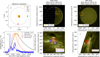 |
Fig. 1. Summary of observations of the SOL2021-05-07T18:43 M3.9 flare. a) Positions of XRT, STIX and the flare (not to scale) as seen from the ecliptic north pole. b) and c) Full-disk views of the Sun in the AIA 1600 Å channel as seen from the positions of STIX and XRT. The orange boxes highlight the flaring active region (NOAA AR 12822). d) Light curves of the flare X-ray emission as measured in the GOES/XRS 1–8 Å channel (black), STIX 22–50 keV (blue) and 6–10 keV (red) bands, and the XRT Be-thick filter (orange). The dashed vertical lines show the interval for which 3D reconstruction was performed. Due to the different light-travel times from the active region to the two spacecraft, the times in this figure have been transformed to light-departure time, i.e. the time at which the emission left the active region. e) and f) Images of the thermal flare loop-top source (red contours) taken by STIX (panel e, 6–10 keV) and XRT (panel f, Be-thick filter), overlaid on AIA 1600 Å observations of the flare ribbons. The non-thermal footpoints imaged by STIX (blue contours, 22–50 keV) are also shown in panel e. |
Figure 1d shows light curves of the flare X-ray emission as measured in the GOES/XRS2 1–8 Å channel (black), the XRT thick beryllium filter (Be-thick; orange), and the STIX 6–10 keV and 22–50 keV bands (red and blue, respectively). The dashed vertical lines show the period for which 3D reconstruction was performed, which includes the latter part of the flare rise phase and the early part of its decay phase. The flare began around 18:39 UT and peaked at M3.9 GOES-class. Due to the difference in light-travel time from the active region to Solar Orbiter and Earth (∼47 s), times throughout this paper, unless otherwise specified, have been converted to the time that the light departed the flare site (“light-departure time”). The Be-thick filter is preferred in this study because its temperature response function overlaps most with the temperatures that dominate the STIX 6–10 keV channels. Hence, the difference in emitting volume seen by both instruments should be negligible for this flare. (For a more detailed treatment of this issue, see Appendix A.1.) We note that the XRT Be-thick and STIX 6–10 keV light curves evolve slightly differently. However, this does not invalidate combining these passbands for 3D reconstruction because different time profiles do not necessarily correspond to different observed source volumes (see Appendix A.1 and Fig. A.2 for a further discussion).
Figures 1e,f show AIA 1600 Å observations of the active region, overlaid with X-ray images of the thermal flare loop-top source (red contours) from the STIX 6–10 keV channels and XRT Be-thick filter, respectively. The X-ray contours in both panels represent 30%, 50%, 70%, and 90% of the brightest X-ray emission in each image. The STIX image, as with all 6–10 keV images in this study, was produced by forward-fitting a single 2D elliptical Gaussian to the STIX visibilities. The STIX indirect-imaging of this flare is particularly well understood, as it was one of the first to be clearly observed (Massa et al. 2022). While the forward-fit image-reconstruction method is not suited to reproducing fine-scale features, it is well suited to retrieving the larger-scale geometry of the source as long as the source is resolved. This is the case for the SOL2021-05-07T18:43 M3.9 flare. Hence, we focus on these larger scales here. For more details of the STIX imaging system and the implications of the different angular resolutions of STIX and XRT, we refer to Appendix A.2 and Massa et al. (2022).
Accurate pointing information is not available from STIX for this flare as its aspect system was not designed to work beyond ∼0.75 AU (Warmuth et al. 2020). Approximate pointing knowledge is provided in these cases by the spacecraft aspect system. More accurate STIX source locations can be determined by shifting the HXR flare footpoints, imaged for this flare using the STIX 22–50 keV emission (blue contours, Fig. 1e), until they line up with the flare ribbons in the reprojected AIA 1600 Å observations. The low altitude of the 1600 Å emission allows us to reproject these images with minimum error, although features observed near the limb as seen from Earth are smeared as a consequence (Fig. 1e). The similarly low altitude of the 22–50 keV emission means that aligning it with UV ribbons gives a good indication of the true STIX pointing. Because STIX uses the same imaging system for all energies, the same alignment shift can be applied to the 6–10 keV emission, even though the altitude of that emission is not known ahead of time. Residual pointing uncertainties are likely to remain. These are accounted for in Sect. 3.2.
Co-temporal STIX-XRT image pairs, such as those shown in Figs. 1e,f, were generated for all times for which XRT Be-thick images were available. Saturated images were excluded as they were found to cause difficulty in defining consistent source boundaries (Sect. 3.2). This left 16 image pairs between 18:48 and 19:01 UT (light-departure time) with a cadence varying from 20 s to two and a half minutes.
3. 3D reconstruction
3.1. Elliptical tie-pointing
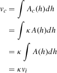
The 3D geometry of the thermal X-ray loop-top source was derived via elliptical tie-pointing. The mathematics of this technique are described in Sect. 4 of Inhester (2006) and have been used by several authors to derive the kinematics of coronal mass ejections (CMEs; e.g. Byrne et al. 2010). Figure 2 (adapted from Fig. 2 of Inhester 2006 and Byrne et al. 2010) demonstrates the technique. First, a series of 2D planes in 3D space (epipolar planes; Fig. 2a) is defined for each image pair. These planes must pass through both observers3 and arbitrary third points, such that the planes cut through the X-ray source. The intersections of the epipolar planes and the source define a series of 2D cross sections. Their locations and extents are calculated by first projecting the epipolar planes onto the images, which, because they pass through both observers, appear as lines. Technically, the planes converge towards the epipole, as shown in Figs. 2a–c. However, the small angular extents of the flare sources cause the planes to be effectively parallel (Fig. 3). Next, the intersections between the source boundary and a single epipolar plane are determined in both observers’ images. These define four infinite lines of sight emanating from the observers, whose intersections define a quadrilateral that bounds the source. The source cross section can then be approximated by inscribing an ellipse in the quadrilateral that is tangent to all four sides (Fig. 2d). A 3D approximation of the X-ray source can then be reconstructed by stacking the elliptical cross sections from multiple epipolar planes (Fig. 2e).
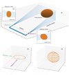 |
Fig. 2. 3D reconstruction via elliptical tie-pointing, adapted from Fig. 2 of Inhester (2006) and Byrne et al. (2010). a) Epipolar planes (blue rectangles) cutting through an X-ray source (elliptical orange spheroid) at progressively steepening angles. By definition, all planes pass through the epipole (dashed line) joining observers 1 (green circle) and 2 (purple circle). b) and c) 2D images of the X-ray source (orange ellipse) as seen by observers 1 and 2, respectively. The different sizes and orientations of the source are due to the source asymmetry and the different viewing angles of the observers. The blue lines show the projections of the epipolar planes onto the images. They converge towards the epipole, but in the case of flare observations, they are effectively parallel because the flare sources are small relative to the source-observer distances. The green and purple points denote the intersections of the epipolar planes with the source boundary. d) Lines of sight tangent to the X-ray source as seen from observers 1 (green) and 2 (purple) in a single epipolar plane. The lines of sight are defined by the intersections of the plane and the source boundary in the images (green and purple points in panels b and c). They form a quadrilateral within which an ellipse is inscribed to represent a cross section of the source. e) Same as panel d, repeated for multiple epipolar planes. By stacking the cross sections (orange ellipses), the X-ray source can be reconstructed in 3D. |
Elliptical cross sections are the simplest model consistent with bi-locational X-ray observations. The optically thin nature of coronal X-ray emission may tempt us to interpret intensity variations as greater source depth along the line of sight. However, these can also be caused by temperature and/or density inhomogeneities. Therefore, no more detailed cross section can be reconstructed without further assumptions.
As well as resulting in quasi-parallel epipolar planes, the small angular sizes of flare X-ray sources also cause the lines of sight from a given observer to be parallel. This results in bounding quadrilaterals that are parallelograms. This makes 3D reconstruction of flare sources different to that of CMEs, whose angular extents tend to result in irregular quadrilaterals. While for irregular quadrilaterals, there is a unique ellipse that can be inscribed tangent to all four sides (Horwitz & Southwest 2002), the symmetry of a parallelogram results in multiple valid solutions. Therefore, to characterise a flare X-ray source cross section, we must further assume that it occupies the maximum possible area. Only then can a unique ellipse be inscribed in the parallelogram (Hayes 2016).
The assumptions that the source is composed of elliptical cross sections that occupy the maximum area consistent with the observations are two important caveats of 3D solar X-ray source reconstruction. The resulting derived volume represents an upper limit of the true source volume. Its discrepancy with the true volume depends on a number of factors, including the angular separation of the observers and the orientation and eccentricity of the source. These can be partially corrected for, and uncertainties between the reconstructed and true source volume can be calculated (see Appendix B.3). This capability reveals that calculating source volumes from stereoscopic observations is an improvement over area scaling from 2D images (Eq. (1)), even when the uncertainties are large. The 2D area scaling technique provides no such mechanism for estimating uncertainties relative to the potential true volume.
3.2. Defining the source boundaries
In order to apply the elliptical tie-pointing technique, the boundaries of the X-ray source must first be established. Because no pre-flare Be-thick observations were available, the XRT flare source boundaries could not be determined by background subtraction. We therefore defined them via the contour threshold at
where  is the median intensity of the image, and
  is the standard deviation of the intensities in the image. Below this level, the enclosed flare area grows disproportionately, and small disconnected contour islands appear. This is due to the inclusion of noise and/or faint disparate emission that does not contribute significantly to the main flare source.
The STIX boundaries were defined by first determining the epipolar planes tangent to the source boundary in the corresponding XRT image (Fig. 3a) and then projecting them onto the STIX image (Fig. 3b). The STIX source boundary was defined by the contour threshold at which the source was tangent to both epipolar planes (solid red contour, Fig. 3b). Since coronal X-ray emission is optically thin, the source must be bounded by the same epipolar planes from both viewing angles, assuming STIX and XRT see the same source. The validity of this assumption depends on the differences in the instruments’ temperature response functions, as well as on the differential emission measure (DEM) of the source and its spatial variation. A detailed discussion of this topic is presented in Appendix A.1 and concludes that the STIX and XRT observations of this event are consistent with both instruments seeing the same source.
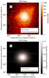 |
Fig. 3. Demonstration of how XRT is used to constrain the source boundary threshold as seen by STIX. a) XRT Be-thick image showing the source boundary (blue contour; Eq. (2)) and the epipolar planes that bound it (green). b) Corresponding 6–10 keV STIX image with three source contours (inner dashed red line: 50%; solid red line: 37%, outer dashed red line: 30%) and the same epipolar planes as in panel a (green) projected to the STIX viewing angle. Only one contour (solid red) is tangent to both bounding epipolar planes and so represents the source boundary as seen by STIX. |
Figure 3b also shows two alternative contour thresholds (dashed red lines). One lies entirely within the bounding epipolar planes, while the other exceeds both. This highlights that there is only one threshold for which the source can be tangent to both planes simultaneously. In some cases, minor pointing adjustments were required to ensure that the STIX source was either tangent to both planes or to neither. This is expected because residual source location uncertainties are expected from the alignment technique used in Sect. 2. However, pointing alterations cannot cause multiple contours to be tangent to both planes simultaneously and so do not affect the validity of this approach.
This technique of determining source boundaries mitigates a number of challenges when comparing instruments with different temperature responses and imaging systems. First, it avoids the need for defining the source boundary in terms of a common photon flux threshold, which would require impractical accuracy in instrument cross-calibration and prior knowledge of the flare spectrum in the spectral range of the Be-thick filter. Second, it circumvents the ambiguity in the STIX source boundary due to its indirect-imaging technique. The STIX images in this study were produced by modelling the source as a 2D elliptical Gaussian, which technically extends to infinity. In most studies of STIX images, arbitrary contour thresholds are sufficient to indicate the location, scale, and orientation of the source. When a specific boundary is required, however, comparison with XRT provides a physically justified choice.
The STIX boundary thresholds calculated in this study had a mean and median of 39% of the image peak intensity and a standard deviation of 4%. It is interesting to note that this is equivalent within the uncertainty to the threshold at which the height of a 2D elliptical Gaussian is z = Ce−1 (37%). The cross section of the elliptical Gaussian at this height, itself an ellipse, has semi-minor and semi-major axes of  and
and  . By inspecting the equation of a 2D elliptical Gaussian,
![$$ \begin{aligned} z = C \exp \left( - \left[ \left( \frac{x}{\sqrt{2} \sigma _a} \right)^2 + \left( \frac{{ y}}{\sqrt{2} \sigma _b} \right)^2 \right] \right), \end{aligned} $$](/articles/aa/full_html/2024/01/aa47212-23/aa47212-23-eq7.gif)
we see that  and
and  are the spatial scales over which the x and y variables are moderated. It therefore represents a natural size scale of the source and provides some mathematical confidence that we have chosen good representations of the true source boundaries in both the STIX and XRT images.
3.3. Deriving the 3D source volume from cross sections
After defining the source boundaries, we applied the elliptical tie-pointing technique to STIX-XRT observations. For each image pair, 51 epipolar planes were defined evenly spaced so that the outer epipolar planes were tangent to the source from both viewpoints (e.g. green lines, Fig. 3). These represented 51 elliptical cross sections per image pair. The volume enclosed by adjacent cross sections was determined via the equation for the volume of a truncated elliptical cone, that is, an elliptical cone without its apex,
![$$ \begin{aligned} v_i = \frac{\pi d}{6} \left[ 2 (a_1 b_1 + a_2 b_2) + a_1 b_2 + a_2 b_1 \right], \end{aligned} $$](/articles/aa/full_html/2024/01/aa47212-23/aa47212-23-eq10.gif)
where d is the 3D distance between the centres of adjacent cross sections, a1 and a2 are the semi-major axes, and b1 and b2 the semi-minor axes of the cross sections. This assumes that the epipolar planes are parallel, which is true to within a fraction of an arcsecond. An estimate of the source volume, Vθϕρ, can be obtained by summing the volumes of all the slices,

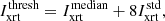
This estimate is an upper limit due to projection effects associated with the observer separation angle and source orientation. A more accurate volume estimate, Vc, can be obtained via

where κ is a correction factor that accounts for these projection effects. It is a function of the observer separation angle from the source, θ, the source orientation angle, ϕ, and the ratio of the minor to major axes of the source cross sections, ρ. A detailed discussion of κ and associated uncertainties is provided in Appendix B. There, we conclude that the optimal observer separation angle for 3D reconstruction via elliptical tie-pointing is 90°. However, uncertainty increases are minimal in the range 90° ± 5° and remain relatively small in the range 90° ± 20°. The observer separation angle relative to the flare site for the SOL2021-05-07T18:43 M3.9 flare was 95.4°, which further emphasises its suitability for 3D reconstruction. We calculated κ for SOL2021-05-07T18:43 M3.9 to be  .
.
3.4. Visualising 3D sources with JHelioviewer
To help visualise the above results and to easily compare them to other observations, we extended the capabilities of JHelioviewer (Müller et al. 2017), a powerful software tool for visualising and analysing solar data. The many capabilities of JHelioviewer include projecting observations onto a sphere, overlaying multiple observations, reprojecting them to different viewing angles, and streaming sequential collections of observations as movies. It also enables overlaying of simple annotations (e.g. crosses, circles, and rectangles) and then modifies them self-consistently as the observations are reprojected. We developed additional annotation geometries and added functionality for drawing shapes from a JSON file. Specifically, JHelioviewer can now visualise stacked ellipses, which enabled us to import the cross sections of the flare X-ray loop-top source into the 3D scene of JHelioviewer. We were then able to inspect the source from any viewing angle, not just those of Hinode and Solar Orbiter, and to compare it to reprojected versions of other common solar observations. Further information can be found in the JHelioviewer documentation4.
Examples are shown in Fig. 4. The thermal X-ray loop-top source is clearly seen as the stack of red ellipses. It is overlaid on an AIA 1600 Å image in Figs. 4a–c, and a Helioseismic and Magnetic Imager magnetogram (HMI; Scherrer et al. 2012) in Fig. 4d. We also show the 22–50 keV STIX observations of the flare footpoints (blue), and an orange semi-ellipse from one footpoint to the other through the centre of the loop-top source. This approximates the flaring loops. The volume correction outlined by Eq. (6) does not help us improve the estimates of the source boundaries. The extent of the source in Fig. 4 therefore is the uncorrected upper limit.
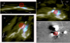 |
Fig. 4. 3D reconstructions created with the observations shown in Figs. 1e,f and visualised using JHelioviewer. The thermal X-ray loop-top source of the flare (stacked red ellipses) is seen from three different viewing angles. Panels c and d show the same viewing angle and field of view. The thermal X-ray source is overlaid on a reprojected AIA 1600 Å image (green, panels a–c) and HMI magnetogram (black/white, panel d). Panels a–c also show elliptical forward-fit STIX images of the non-thermal flare footpoints (blue) as seen in 22–50 keV. The orange line in all panels is a semi-ellipse drawn between the footpoints through the centre of the thermal source as an approximation of the flare loops. The X-ray footpoint sources are omitted from panel d to give a clearer view of the magnetogram, but their locations can be inferred from the ends of the orange loop. For reference, the green and red lines show the heliocentric Stonyhurst lines of latitude and longitude, and each panel shows the north-west axes in its corners. |
Figure 4 reveals the full 3D nature of the thermal X-ray loop-top source of the flare. It sits between and above the footpoints, consistent with the standard flare model (Sect. 1). The X-ray footpoints are aligned with the AIA 1600 Å flare ribbons, as required by the co-alignment process. Figure 4d, which shows the same viewing perspective and field of view as Fig. 4c, reveals that the loop-top source straddles a photospheric magnetic polarity inversion line and that the more intense easterly footpoint corresponds to a region of negative polarity that is wedged between two regions of positive polarity.
4. Results
4.1. Testing the area-to-volume scaling law
The solid black line in Fig. 5a represents the corrected 3D source volume (Eq. (6), Fig. B.5b) as a function of time. The dotted black lines show the upper and lower limits of the uncertainty range that is twice as likely to contain the true volume as to exclude it (see Appendix B for a derivation of this uncertainty range and the assumptions underlying it). The true volume is equally likely to lie between the solid and upper dotted curves as between the solid and lower dotted ones, despite the asymmetry of the uncertainty range. The blue and orange curves show the volume estimated by applying Eq. (1) to the source areas in the STIX and XRT images, respectively. The same source boundaries were used as in the 3D analysis. The area-scaled volumes exceed the 3D-derived volume at all times. Moreover, except for the XRT volume between roughly 18:56 and 19:00, they also exceed the uncertainty range. Figure 5b more closely examines these overestimates. The blue and orange curves show the STIX and XRT area-scaled volumes normalised by the 3D-derived volume (solid lines) and the 3D uncertainty range (dotted lines).
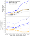 |
Fig. 5. a) Temporal evolution of the X-ray loop-top source volume of the SOL2021-05-07T18:43 M3.9 flare. The 3D-derived volume (solid black curve) is compared to those derived from the traditional area-to-volume scaling law (Eq. (1)) based on the STIX 6–10 keV (blue curve) and XRT Be-thick (gold curve) images. The dotted black curves show the range within which the true source volume is twice as likely to lie based on the geometric uncertainties of the 3D reconstruction method. b) STIX- (blue curve) and XRT-area-scaled volumes (gold curve) normalised by the 3D-derived volume. The dotted lines show the area-scaled volumes normalised by the 3D volume uncertainty range. |
Figure 5 emphasises that the area-scaled volumes overestimate the true volume by a factor of 1–1.4 for XRT and 1.4–2 for STIX. When considering the uncertainty range of the 3D-derived volume, these factors expand to 0.9–1.8 for XRT and 1.3–2.5 for STIX. This demonstrates that Eq. (1) may overestimate the true volume of this flare by over a factor of 2. An alternative area-to-volume scaling law used by some previous studies (e.g. Warmuth & Mann 2013) assumes a spherical source,
This leads to volume estimates that are lower by a factor of ≈0.75, which results in a better agreement with the 3D-derived volume for this particular flare. It should be noted that the 3D analysis in this study suggests that this X-ray source is fairly spherical. Therefore, the discrepancy between the true volume and area-scaled estimates could be greater for more elongated sources. Nonetheless, given a single viewing angle, Eq. (7) produces better volume estimates than Eq. (1) for the SOL2021-05-07T18 M3.9 flare, and likely for many others.
Figure 5 reveals further complications, however, that cannot be resolved by simply adjusting the area-to-volume scaling factor. The overestimations of the area-scaled volumes vary with time and evolve differently depending on the different viewing angle. The STIX-area-scaled volume overestimate is greater than that of XRT. The indirect-imaging technique of STIX may play a role. However, because the boundaries of the STIX source were defined with reference to the size of the XRT source, it is likely that the asymmetry of the source is more significant. This is supported by the fact that the blue and orange curves in Fig. 5b move slightly out of phase. This suggests that the volume of the source evolves differently in the dimensions to which the different observing perspectives are sensitive. This issue will likely be more pronounced for sources that are less spherical than the one studied here. This emphasises the importance of multi-viewpoint observations for gaining a fuller understanding of the geometry and evolution of thermal X-ray loop-top sources in solar flares.
4.2. 3D evolution of the thermal X-ray loop-top source
4.2.1. Spatio-temporal evolution
The online movie reveals the 3D evolution of the thermal X-ray loop-top source from multiple viewing angles in relation to other (E)UV and non-thermal HXR features. The upper and lower left panels show AIA 171 Å and 1600 Å observations, respectively, as seen from Earth. The right panels show AIA 1600 Å observations reprojected to viewing angles from above (upper right) and south-east of (lower right) the flare site. Non-thermal HXR footpoints observed by STIX in the 22–50 keV range are shown in blue, and the 3D-reconstructed thermal X-ray loop-top source is shown as stacks of red ellipses. We recall that the volume correction (Eq. (6)) cannot be applied to the source boundaries, and therefore, the extent of the source seen in the right panels of the movie are upper limits.
Before the flare, AIA 171 Å shows highly inclined coronal loops. At 18:42, approximately coincident with the appearance of the first non-thermal emission, an S-like ribbon is activated in both the 171 Å and 1600 Å images. The coronal loops seen in AIA 171 Å become more inclined and appear to part and erupt around 18:46, while the south-west arm of the ribbon takes on a circular shape in 1600 Å as shown in the top right panel. Strong 171 Å emission is also seen from this region at the same time. As the overlying AIA 171 Å loops erupt, bright emission is seen from the apex of the underlying loops, which subsequently dim and contract. Throughout this time, the non-thermal footpoints move around, but mainly straddle the northern kink of the ribbon. The eastern footpoint is often much fainter than the western one. At 18:48, 3D reconstruction becomes possible. Hot plasma was present before this (red light curve, Fig. 1d), but could not be reconstructed due to the lack of XRT Be-thick observations. At 18:48, no coronal 171 Å emission appears to be associated with the 3D thermal X-ray source. Only one non-thermal footpoint is clearly visible, possibly because the footpoints have moved too close together to be separated by the angular resolution of STIX and/or because the difference in their relative intensities is too great for the imaging dynamic range of STIX. The thermal source sits above and slightly to the south-east of the footpoints, approximately in line with the inclination of the coronal structures in the core of the active region, as seen by AIA 171 Å. This changes at approximately 18:49, when intense emission is seen in 171 Å that is aligned with the thermal X-ray source as seen from Earth. Two non-thermal footpoints are clearly visible. They have moved slightly south and straddle the northern kink of the ribbon. Around 18:53, the eastern footpoint disappears, to be replaced by another in the south-west arm of the ribbon (or an elongation of the western footpoint in that direction). The thermal source volume begins to grow and becomes clearly asymmetric. Additional thermal emission extends above the newly formed non-thermal footpoint. The thermal source rises in altitude along with the intense 171 Å emission, which begins to resemble coronal loop-top emission rather than emission associated with the flare ribbon. A twisted outflow from the flare is also seen in AIA 171 Å and faint higher-altitude loops expand outwards. Shortly before 18:56, the non-thermal X-ray emission becomes too faint for reliable imaging, and the blue sources disappear from the movie. The thermal X-ray source continues to rise and deform asymmetrically as the flare enters its decay phase. Shortly after 19:00, XRT Be-thick observations are no longer available, and the thermal X-ray source disappears. However, hot plasma remains as the flare continues to evolve and cool (red light curve, Fig. 1d).
This movie demonstrates the power of 3D reconstruction for understanding flare X-ray sources in relation to the rest of the active region. Although we did not perform a 3D reconstruction of the EUV flare loops, their timing and alignment with the thermal X-ray source as seen from Earth give us an indication of their 3D position. Furthermore, the movie shows how the position of the thermal X-ray source evolves in relation to the flare ribbon and how it deforms asymmetrically in response to the changing locations of the non-thermal X-ray footpoints.
4.2.2. Kinematic and thermodynamic evolution
Figure 6 shows the kinematic and thermodynamic evolution of the thermal X-ray loop-top source of the flare. The dotted vertical line in all panels shows the time of the peak in the GOES/XRS 1–8 Å channel and acts as a demarcation between the flare rise and decay phases.
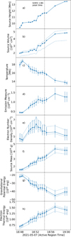 |
Fig. 6. Temporal evolution of the thermal X-ray loop-top source of the SOL2021-05-07T18:43 M3.9 flare. a)–d) Source height, volume, and STIX-derived temperature and emission measure. The dotted lines in panel b have the same meaning as in Fig. 5a. The error bars in panels c,d represent the fitting uncertainties to the STIX spectra. e)–h) Source-averaged electron number density, mass, gravitational potential energy, and electron thermal energy derived from panels a–d. The dotted lines represent the uncertainty due to volume alone, and the error bars denote the combined volume and spectral fit uncertainties. |
Figure 6a shows the height of the source centre above the solar surface as a function of time. When the XRT Be-thick observations begin, the source is at 9.3 Mm. It rises at an approximately constant rate during late rise and early decay phases, reaching 13.5 Mm after approximately 12 min. When the XRT Be-thick observations cease, there is no strong indication that the motion is abating. The height increase is presumably due to the heating of flaring loops that reconnect at progressively higher altitudes. The apparent velocity of the X-ray source is ∼6.3 km s−1. This is comparable to previous single-viewpoint studies, including Gallagher et al. (2002) and Milligan et al. (2010). These studies examined the motions of the thermal X-ray loop-top source in an X- and C-class flare, respectively. Both flares were observed at the solar limb, where altitude projection effects are minimal. Gallagher et al. (2002) found an apparent velocity of 10 km s−1, which was observed to be slightly faster than the growth of the EUV loops observed by TRACE (Transition Region And Coronal Explorer). Milligan et al. (2010) found an apparent rise rate of 5 km s−1. The approximate agreement with these studies indicates that our 3D reconstruction method reproduces reliable positions and dynamics without requiring the flare to be observed at the solar limb.
Figure 6b shows the same corrected 3D-derived volume of the thermal X-ray loop-top source as shown by the solid black line in Fig. 5. The dotted lines represent the same uncertainty interval. Although XRT Be-thick observations are only available towards the end of the rise phase, significant volume growth is not apparent until several minutes before the GOES/XRS 1–8 Å peak. The volume continues to grow into the decay phase, after which it appears to stabilise.
Figures 6c,d show the temperature and volumetric emission measure (EM) derived from spectral fits to the STIX observations at the times of the STIX-XRT image pairs. The emission measure is analogous to the amount of emitting material and is defined as  , where ne is the electron number density, and dV is the 3D volume element5. The remaining panels in Fig. 6 show the evolution of the thermodynamic properties derived from panels a–d. The dotted lines represent the volume uncertainty interval folded through the derivations, and the error bars show the volume uncertainties combined with the STIX spectral fitting uncertainties associated with the temperature and/or emission measure, as appropriate.
Figure 6e shows the evolution of the electron number density, ne, derived via

where EM is the volumetric emission measure. Equation (8) assumes a volume filling factor of unity and so represents the spatially averaged density within the source. Higher and lower densities may exist more locally and may evolve slightly differently. Figure 6e shows that the source-averaged density increases from 4.7 × 1010 cm−3 to 6.5 × 1010 cm−3 in the space of four minutes. It peaks before the GOES/XRS 1–8 Å peak. The density begins to fall as the volume begins to increase significantly. The cause of this is revealed by comparing the density and volume with the X-ray source mass, shown in Fig. 6f. This was derived by assuming that the plasma consists of an equal number of electrons and protons and by applying the equation
where me and mp are the electron and proton masses, respectively. Higher-mass elements were neglected. The resulting mass time-profile shown in Fig. 6f reveals that material continues to be injected into the X-ray source volume. However, the rate of the mass increase is lower than the rate of the volume increase after approximately 18:54 UT. Only shortly before 19:00 UT does the mass increase stop. This is also approximately the time at which the volume stabilises.
Figure 6g shows the gravitational potential energy, U, of the thermal X-ray loop-top source derived via

where G is the gravitational constant, M is the mass of the Sun, m is the mass of the X-ray source (Fig. 6f), and R is the distance of the X-ray source from the centre of the Sun. The gravitational potential of the source is on the order of 1031 erg, and the evolution of its magnitude approximately mimics that of the mass.
The solid blue curve in Fig. 6h shows the instantaneous thermal energy of the X-ray source as a function of time, derived via
where kB is the Boltzmann constant, and T is the source temperature (Fig. 6c). The thermal energy rises from 7 × 1029 erg at 18:48 UT, when XRT Be-thick observations begin, to 1.5 × 1030 erg around 18:57 UT, a few minutes after the peak in the GOES/XRS 1–8 Å channel. This represents an increase of a factor of 2. After this time, the thermal energy begins to reduce as the continued heating of the flare plasma is overtaken by the cooling mechanisms.
Comparison of the error bars (total uncertainties) and dotted lines (volume-associated uncertainties) in Figs. 6e–h reveals that the volume is the dominant uncertainty factor. This further highlights the importance of deriving volumes from multi-viewpoint observations. By contrast, area-scaled volume estimates do not provide a way to judge the reliability of derived properties and hence of the scientific conclusions we draw from them.
5. Conclusions
We have reconstructed the 3D position and volume of a thermal flare X-ray loop-top source as a function of time (Sects. 3.2 and 3.3). This was achieved by applying an elliptical tie-pointing technique (Sect. 3.1) to co-temporal imaging observations from Hinode/XRT (Be-thick filter) and Solar Orbiter/STIX (6–10 keV; Sect. 2).
The differences in the designs and temperature sensitivities of these instruments resulted in a number of complexities. However, we showed that these can be mitigated or overcome in certain circumstances, including the SOL2021-05-07T18:43 M3.9 flare examined in this study (Appendix A). Nonetheless, careful consideration should be given on a case-by-case basis before combining STIX and XRT observations for 3D reconstruction. Projection effects associated with the 3D reconstruction technique were also explored (Appendix B). It was shown that the optimal observer separation angle for 3D reconstruction via elliptical tie-pointing, that is, those associated with the smallest uncertainties due to projection effects, is 90° ± 5°. However, the uncertainties remain relatively small in the range 90° ± 20°. 3D reconstruction is still viable at other separation angles, provided the higher associated uncertainties are sufficient for the science case.
The 3D volume derived for the SOL2021-05-07T18:43 M3.9 flare was compared to what would have been derived using the traditional area-to-volume scaling law if only STIX or XRT observations had been available (Sect. 4.1, Fig. 5). It was found that these volumes can overestimate the 3D-derived volume by over a factor of 2. Moreover, the degree of overestimation varied with time and viewing angle. It was determined that this was not primarily due to the different imaging techniques of the instruments, but to the asymmetric evolution of the X-ray source. Better area-scaled volume estimates were found by assuming a spherical source (Eq. (7)), but this could not correct for the asymmetric volume evolution. These issues demonstrate the value of 3D reconstruction over traditional single-viewpoint volume estimates for understanding the thermodynamics and kinematics of thermal flare X-ray loop-top sources.
Various properties of the thermal X-ray loop-top source were then derived from the 3D position and volume and STIX-derived temperature and emission measure (Sect. 4.2.2, Fig. 6). These included the density, mass, gravitational potential energy, and thermal energy. The apparent upward velocity of the source was ∼6.3 km s−1, which is in line with previous limb observations of similar X-ray loop-top sources. This indicates that 3D reconstruction via elliptical tie-pointing leads to reasonable positions and dynamics without requiring that observations be made at the limb. The 3D reconstruction technique and spectrally derived temperature and emission measure enabled observationally constrained uncertainties to be assigned to the thermodynamic properties of the loop-top source. Within these, the volume-related uncertainties dominated. Volumes estimated by scaling 2D projected areas do not provide such a method for determining uncertainties. Therefore, even when the uncertainties are large, 3D-derived volumes are beneficial because they provide an indication of the reliability of the volume measurements and properties derived from them.
Finally, this study led to the development of new capabilities in JHelioviewer for importing and visualising 3D sources and comparing them with other observations (Sect. 3.4, Fig. 4, Sect. 4.2.1, and online movie). Users who would like to avail themselves of these features should see the latest version of the user manual (footnote 4).
Movie
Movie 1 associated with Fig. 4 (20210507_3Dthermalxray_171A_1600A_nonthermalxray) Access here
The line joining the observers is called the epipole (dashed line Fig. 2a), hence the term epipolar plane.
Emission measure can also be defined in terms of distance along the line of sight, i.e. column EM, as 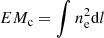 where dl is the line-of-sight length element. However this form is only useful from a specific observer’s point-of view. Therefore, in this paper we will use volume emission measure unless otherwise stated.
Acknowledgments
This work was conducted using tools provided by the SunPy (Mumford et al. 2020), AstroPy (Astropy Collaboration 2018, 2013) and JHelioviewer projects (Müller et al. 2017), funded by ESA Contract No. 4000107325/12/NL/AK, High Performance Distributed Solar Imaging and Processing System. Solar Orbiter is a space mission of international collaboration between ESA and NASA, operated by ESA. The STIX instrument is an international collaboration between Switzerland, Poland, France, Czech Republic, Germany, Austria, Ireland, and Italy. D.F.R., A.F.B., and S.K. are supported by the Swiss National Science Foundation Grant 200021L_189180 and the grant ‘Activités Nationales Complémentaires dans le domaine spatial’ REF-1131-61001 for STIX. Hinode is a Japanese mission developed and launched by ISAS/JAXA, with NAOJ as domestic partner and NASA and STFC (UK) as international partners. It is operated by these agencies in co-operation with ESA and NSC (Norway).
References
- Aschwanden, M. J., Boerner, P., Ryan, D., et al. 2015, ApJ, 802, 53 [Google Scholar]
- Astropy Collaboration (Robitaille, T. P., et al.) 2013, A&A, 558, A33 [NASA ADS] [CrossRef] [EDP Sciences] [Google Scholar]
- Astropy Collaboration (Price-Whelan, A. M., et al.) 2018, AJ, 156, 123 [Google Scholar]
- Byrne, J., Maloney, S., McAteer, J., Refojo, J., & Gallagher, P. 2010, Nat. Commun., 1, 74 [NASA ADS] [CrossRef] [Google Scholar]
- Cargill, P. J., Mariska, J. T., & Antiochos, S. K. 1995, ApJ, 439, 1034 [NASA ADS] [CrossRef] [Google Scholar]
- Carmichael, H. 1964, NASA Spec. Pub., 50, 451 [NASA ADS] [Google Scholar]
- Emslie, A. G., Dennis, B. R., Shih, A. Y., et al. 2012, ApJ, 759, 71 [Google Scholar]
- Gallagher, P. T., Dennis, B. R., Krucker, S., Schwartz, R. A., & Tolbert, A. K. 2002, Sol. Phys., 210, 341 [NASA ADS] [CrossRef] [Google Scholar]
- Golub, L., Deluca, E., Austin, G., et al. 2007, Sol. Phys., 243, 63 [NASA ADS] [CrossRef] [Google Scholar]
- Hayes, M. J. D. 2016, Proc. Canad. Soc. Mech. Eng. Int. Congr., 2016 [Google Scholar]
- Horwitz, A., & Southwest, J. 2002, Pure Appl. Math., 2002, 6 [Google Scholar]
- Inhester, B. 2006, ArXiv e-prints [arXiv:astro-ph/0612649] [Google Scholar]
- Kano, R., Sakao, T., Hara, H., et al. 2008, Sol. Phys., 249, 263 [NASA ADS] [CrossRef] [Google Scholar]
- Kopp, R. A., & Pneuman, G. W. 1976, Sol. Phys., 50, 85 [Google Scholar]
- Kosugi, T., Matsuzaki, K., Sakao, T., et al. 2007, Sol. Phys., 243, 3 [Google Scholar]
- Krucker, S., Hurford, G. J., Grimm, O., et al. 2020, A&A, 642, A15 [NASA ADS] [CrossRef] [EDP Sciences] [Google Scholar]
- Lemen, J. R., Title, A. M., Akin, D. J., et al. 2012, Sol. Phys., 275, 17 [Google Scholar]
- Massa, P., Battaglia, A. F., Volpara, A., et al. 2022, Sol. Phys., 297, 93 [NASA ADS] [CrossRef] [Google Scholar]
- Milligan, R. O., McAteer, R. T. J., Dennis, B. R., & Young, C. A. 2010, ApJ, 713, 1292 [NASA ADS] [CrossRef] [Google Scholar]
- Müller, D., Nicula, B., Felix, S., et al. 2017, A&A, 606, A10 [Google Scholar]
- Müller, D., St. Cyr, O. C., Zouganelis, I., et al. 2020, A&A, 642, A1 [Google Scholar]
- Mumford, S., Freij, N., Christe, S., et al. 2020, J. Open Source Softw., 5, 1832 [NASA ADS] [CrossRef] [Google Scholar]
- Pesnell, W. D., Thompson, B. J., & Chamberlin, P. C. 2012, Sol. Phys., 275, 3 [Google Scholar]
- Ryan, D. F., Milligan, R. O., Gallagher, P. T., et al. 2012, ApJS, 202, 11 [NASA ADS] [CrossRef] [Google Scholar]
- Ryan, D. F., Chamberlin, P. C., Milligan, R. O., & Gallagher, P. T. 2013, ApJ, 778, 68 [NASA ADS] [CrossRef] [Google Scholar]
- Scherrer, P. H., Schou, J., Bush, R. I., et al. 2012, Sol. Phys., 275, 207 [Google Scholar]
- Sturrock, P. A. 1966, Nature, 211, 695 [Google Scholar]
- Warmuth, A., & Mann, G. 2013, A&A, 552, A86 [NASA ADS] [CrossRef] [EDP Sciences] [Google Scholar]
- Warmuth, A., Önel, H., Mann, G., et al. 2020, Sol. Phys., 295, 90 [NASA ADS] [CrossRef] [Google Scholar]
Appendix A: Challenges in combining XRT & STIX and their mitigations
Observations used for 3D reconstruction should ideally be made with identical telescopes operating in the same mode. This ensures that differences in the projected source morphology are solely due to the different viewing angles. Because this is currently not available in the X-ray regime, this study combines two non-identical instruments: XRT (Golub et al. 2007; Kano et al. 2008) and STIX (Krucker et al. 2020). Their differences lead to a number of challenges and caveats. In this appendix, we outline the most significant of these and discuss mitigation strategies.
A.1. Temperature responses
The most important requirement for combining instruments for 3D reconstruction is that they observe the same emitting volume. In the case of thermal emission, this is determined by two main factors. The most important is the temperature response functions of the instruments6. Figure A.1 shows the temperature response functions for the highest-temperature filters of XRT and of the STIX 6 – 10 keV band. It is clear that none of the XRT temperature responses are the same as that of STIX. The second factor is the spatial DEM distribution78 of the X-ray source. Instruments with different temperature responses will see the same emitting volume if
-
the DEM is spatially uniform throughout the source, or
-
the instrument response functions overlap sufficiently at the dominant plasma temperature(s).
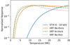 |
Fig. A.1. Normalised temperature response functions for the STIX 6 – 10 keV band (solid blue) and the highest-energy XRT filters: Be-thick (solid orange), Al-thick (dashed green), and Be-thin (dotted red). The Be-thick filter overlaps most with the STIX 6 – 10 keV response. |
It is rare for either of these conditions to be strictly true in the solar atmosphere. However, they can be approximately satisfied if the spatial DEM in the temperature regimes of both instruments decreases fast enough near the edge of the source. The chance of this is increased the greater the overlap of the response functions.
With this in mind, we again consider Figure A.1. Although the XRT and STIX response functions are different, the XRT Be-thick response is fairly flat above ∼10 MK and begins to decrease rapidly below ∼5 MK. Typically, only hot flaring loops exceed 5 MK, and the bulk of the flare plasma rarely exceeds 25 MK (Ryan et al. 2012). Even at this temperature, the XRT Be-thick is significantly responsive. In comparison, STIX is responsive to temperatures ≳ 8 MK. This overlap provides ample opportunity for the above second condition to be fulfilled. Moreover, flaring loops typically have a temperature gradient, with the hottest plasma at the top. Therefore, the temperatures dominating the XRT and STIX responses will occupy almost the same volume in many cases. An example is presented in Figure A.2, which shows XRT and STIX observations near the peak of the SOL2021-11-01T23:40 C4-class flare. The black and red image shows the XRT Be-thick emission. The white lines show 30% to 90% contours of the 6–10 keV STIX emission. The STIX image was produced in the same way as for the SOL2021-05-07 M3.9 flare, namely by forward-fitting a single elliptical Gaussian to the visibilities. At this time, Solar Orbiter was close to Earth, meaning that both instruments should have seen the same flare area if they observed the same emitting plasma. This is the case in Figure A.2a, demonstrating that at least in some cases, XRT and STIX do see the same flare volume. Figure A.2b shows the temporal evolution of the normalised XRT Be-thick and STIX 6 – 10 keV emission, which are similar, but not identical. The Be-thick emission evolves more slowly and peaks later than 6 – 10 keV. This is the same qualitative behaviour as in the SOL2021-05-07T18:43 M3.9 flare (Figure 1d). Despite this, the source sizes still agree well, demonstrating that different time profiles do not necessarily correspond to different observed source volumes. This could be due to one of the scenarios enumerated in the previous paragraph, or to a combination of both.
 |
Fig. A.2. a) X-ray image of a C4 flare that peaked at 2021-11-01 23:39 UT as observed at Earth. The red and black show the XRT Be-thick filter image, and the white lines show 30%–90% contours of the STIX 6 – 10 keV emission. The STIX image was produced by forward-fitting an elliptical Gaussian, and its size has been corrected for the difference in observer distance. Despite the different temperature responses and imaging techniques of the two instruments, the source areas agree very well. b) Light curves of the STIX 6 – 10 keV (solid blue) and XRT Be-thick (dashed orange) emission. The source size in panel a) agrees despite a slightly different evolution of the light curves. |
The above agreements are comforting, but direct comparisons like this can only be performed for flares that are observed from the same viewing angle. By definition, 3D reconstruction cannot be performed with such observations. Therefore, we would like an analogous test for flares observed from different viewing angles. One option is to determine whether the intensities observed by both instruments are consistent with the same temperature and emission measure. The first step is to derive the flare temperature, Tstix, and volume emission measure, EMstix, by forward-fitting the STIX spectrum. These properties are then combined with the XRT Be-thick temperature response function, Rxrt(T), to predict the XRT intensity,  ,
,
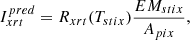
where Apix is the area of an XRT pixel projected to the source distance. The predicted intensity can then be compared to the observed XRT Be-thick intensity,  , obtained by summing the observed intensities in the flaring pixels,

where Ii is the Be-thick intensity in the ith flaring XRT pixel.
We applied this strategy to the SOL2021-05-07T18:43 M3.9 flare and found that the predicted and observed XRT intensities agree to within 40% on average during the period of 3D reconstruction. Tight agreement is not expected given the uncertainties associated with the temperature response functions of broadband imagers such as XRT. Therefore, this result suggests that the XRT- and STIX-observed intensities are roughly consistent with emission from the same amount of emitting material at the same temperature.
A.2. Imaging techniques and performance
XRT and STIX employ very different imaging techniques. XRT directly focuses X-rays onto non-spectroscopic pixelated detectors using grazing-incidence X-ray focusing optics. Images at different temperatures are produced by placing transmission filters in front of the detectors. By contrast, STIX provides X-ray imaging spectroscopy in the range 4–150 keV. Due to the difficulty of focusing X-rays in this regime, STIX employs an indirect-imaging technique. Spatial information is encoded in moiré patterns whose amplitude and phase depend on the location, size, and orientation of the X-ray source. The moiré patterns are cast by pairs of slightly offset absorbing grids of slits and slats onto spectroscopic pixelated photon-counting detectors. A single grid pair and detector together are known as a subcollimator. Each subcollimator samples an angular scale on the sky corresponding to its slit width and pitch in the direction perpendicular to the long axis of its slits. STIX samples ten angular scales from 7”–180”, each at three orientations. Hence, images can be reconstructed by combining these image components via Fourier-based algorithms, as is done in radio interferometry.
The performance consequences of these different designs lead to a number of complications when combining and interpreting the images. The first is differing angular resolutions. The finest grids of STIX correspond to 7”, which is much larger than the 2" FWHM angular resolution of XRT. Consequently, STIX cannot be used to estimate the area or volume of an X-ray source on spatial scales < 14”. This is mitigated by the fact that Solar Orbiter approaches closer to the Sun than Earth. Table A.1 shows the spatial resolutions that correspond to the angular resolution of each instrument at 1 AU from Sun centre. It also shows the STIX resolution at a distance from Sun centre of 0.92 AU (Solar Orbiter’s distance on 2021 May 7) and 0.28 AU (Solar Orbiter’s closest approach). In the latter case, the spatial resolutions of STIX and XRT are the same. However, due to orbital mechanics, Solar Orbiter spends more time near aphelion than perihelion. Therefore, more flares are expected to be observed at coarser spatial resolution with STIX than with XRT. Nonetheless, as long as the size scale of the X-ray source is greater than 14” from the STIX observing position and 4” from that of XRT, as is the case for the SOL2021-05-07T18:43 M3.9 flare, the derived volume is not compromised by insufficient resolution.
Spatial resolution of XRT compared to that of STIX at different distances from Sun centre.
Although the smallest angular scale of STIX is 7”, it is only sampled at three orientations on the plane of the sky. This limits the fine structure that STIX can resolve, even on the 7” scale. This is mitigated at larger angular scales by the fact that different sets of orientations are used at different scales. Nonetheless, the STIX imaging is better suited to determining the general morphology of a source than the fine-scale structure discernible by XRT. Hence, users should not attempt to capture this structure in their 3D reconstructions. For example, fitting or smoothing the boundary of the XRT source may simplify the reconstruction and likely will not sacrifice granular detail that could otherwise be reliably reconstructed.
Appendix B: Interpreting derived 3D volumes
B.1. Relationship between the derived 3D volume and projection effects of its 2D cross sections
The 3D volumes reconstructed in this study are composed of stacks of 2D elliptical cross sections, where the first-order volume estimate is made by summing the volumes between the cross sections (Equations 4 and 5). However, the areas of the elliptical cross sections are upper limits, due to projection effects that are related to the observer angle and to the source orientation and eccentricity. As we show below, these effects can be corrected for to within a degree of uncertainty. Let the correction factor for the cross-section area be κ. We refer to this as the area scaling factor. A corrected estimate of an elliptical cross section, Ac, can be estimated by

Now note that the volume between two stacked parallel ellipses (equivalent to Equation 4) is given by
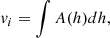
where h is the distance between the ellipse centres, and A(h) = πa(h)b(h) is the area of the elliptical cross section as a function of h. Assuming that κ is independent of h, a corrected estimate of the inter-cross-section volume, vc, can be given by
. Summing the volumes between multiple stacked cross sections gives the total volume of the source. Hence, combining Equations B.3 and 5 gives Equation 6. This demonstrates that the correction factor and uncertainty in the derived 3D volume is determined by the those of the cross sections. In the following subsections, we derive the area scaling factor, κ, in the 2D case and use it to derive the area uncertainties. These can then be trivially extended to 3D volumes.
B.2. Effects of observer separation angle and source geometry on the derived cross-section area
Consider Figure B.1. The solid ellipse represents a 2D cross section of a 3D source formed by an epipolar plane. For brevity, we simply refer to the 2D cross section as “the source”. The source has a semi-major axis, a, and a semi-minor axis, b. It is seen by two observers, 1 and 2, which, by definition, lie in the same 2D epipolar plane and are separated by an angle, θ, relative to the centre of the source. Each observer is assumed to be sufficiently distant so that their lines of sight tangent to the source (dotted black lines) are parallel. For convenience and without loss of generality, we define a Cartesian coordinate system whose origin is located at the centre of the source and whose x-axis is aligned with the lines of sight of observer 1. The source orientation, ϕ, is the counterclockwise angle from the x-axis to the source major axis. The intersections of the lines of sight tangential to the source define a bounding parallelogram (solid black lines). Because the geometry of the source is not known from the observations, it is approximated by the maximum-area ellipse inscribed in the parallelogram (dashed ellipse), as described in Section 3.1. We call this “the derived ellipse” and its area “the derived area”.
 |
Fig. B.1. Difference between the true cross-sectional geometry of a source (solid ellipse) and the maximum-area (dashed) ellipse derived from observations taken by two observers separated by an angle θ. The source has semi-major and semi-minor axes a and b, and an orientation angle, ϕ, between its semi-major axis and the lines of sight of observer 1. The derived ellipse has conjugate diameters, d1 and d2, with the same lengths as the parallel sides of the bounding parallelogram (solid lines) formed by the tangential lines of sight (dotted lines). The solid blue line represents the x-axis, and the dotted orange line represents the distance, 2c1, between the lines of sight from observer 1. |
The derived ellipse has the same centre as the source, but its boundaries and area can differ. It can be shown that only at θ = ±90° and ϕ = n90° where n ∈ ℤ, is the derived ellipse equivalent to the source. That is to say, they have the same orientation, semi-axes, and boundary. However, while θ is known, ϕ cannot be determined from X-ray observations due to projection effects and the optically thin nature of coronal X-ray emission. Therefore, we must understand how the derived area depends on source orientation and eccentricity. This is described by the area scaling factor, which is defined as
![$$ \begin{aligned} \kappa = \frac{A_{0}}{A_{\theta \phi \rho }} = \frac{\sin ^2\theta }{\sqrt{\left(\sin ^2\phi + \rho ^2 \cos ^2\phi \right) \left[\frac{1}{\rho ^2} \left( \frac{\sin \phi }{\tan \theta } + \cos \phi \right)^2 + \left(\frac{\cos \phi }{\tan \theta } + \sin \phi \right)^2 \right],}} \end{aligned} $$](/articles/aa/full_html/2024/01/aa47212-23/aa47212-23-eq28.gif)
where A0 is the source area, Aθϕρ is the derived area, and ρ = b/a is the ratio of the semi-axes of the source. The area scaling factor can be broken into two components, κ = κθϕρsin2θ, where
![$$ \begin{aligned} \kappa _{\theta \phi \rho }= \frac{1}{\sqrt{\left(\sin ^2\phi + \rho ^2 \cos ^2\phi \right) \left[\frac{1}{\rho ^2} \left( \frac{\sin \phi }{\tan \theta } + \cos \phi \right)^2 + \left(\frac{\cos \phi }{\tan \theta } + \sin \phi \right)^2 \right]}} \end{aligned} $$](/articles/aa/full_html/2024/01/aa47212-23/aa47212-23-eq29.gif)
(see Appendix B.5 for the derivation of this equation). The angle θ can be unambiguously determined from the positions of the observers. Therefore, in order to correct for projection effects and understand the inherent uncertainties involved, we must determine κθϕρ, which we refer to as the orientation area scaling factor.
Figure B.2 shows Equation B.5 as a function of ϕ for several separation angles and two semi-axis ratios. First, consider the semi-axis ratio of ρ = 0.5 (Figure B.2a). The curves are periodic over an interval of 180°. At θ = 90°, the curve is symmetric about 45° and periodic over 90°. As θ decreases, a periodicity over ϕ = 180° is maintained. However, the trough at ϕ < 90° diminishes and the trough at ϕ > 90° grows and shifts towards 90°. (This behaviour is reversed as θ increases from 90° towards 180°.) As θ approaches 0° (and 180°), the curve becomes single-troughed, its amplitude grows further, and it eventually shifts to ϕ = 90°. All curves equal 1 at some value of ϕ, indicating that the true source area can be calculated from any separation angle provided the source has an appropriate orientation. However, the θ = 90° curve has the smallest trough and therefore results in the smallest maximum difference between the derived and source areas. The same qualitative behaviour is seen for a semi-axis ratio of ρ = 0.25 in Figure B.2b. The quantitative difference is that the amplitude(s) of the curves are greater, which likewise implies a greater possible discrepancy between the derived and true source areas. Nonetheless, the smallest maximum discrepancy is also achieved θ = 90°. This indicates that the optimal observer separation angle is θ = 90°.
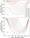 |
Fig. B.2. Area scaling factor (Equation B.5) as a function of source orientation, ϕ, and observer separation angle, θ, for two source semi-axis ratios, ρ = 0.5 (a) and ρ = 0.25 (b). The closer ρ is to 1 and the closer θ is to 90° the smaller the scaling factor, i.e. the closer the derived area is to the source area. The dashed green-yellow curves at 95.4° represent the separation angle of STIX and XRT relative to the flare X-ray source of SOL2021-05-07T18:43 M3.9. |
B.3. Correcting cross-section areas for observer separation and source geometry
As already stated, the source orientation, ϕ, and semi-axis ratio, ρ, cannot be determined from X-ray observations due to projection effects and the optically thin nature of solar X-ray emission. Therefore, the utility of Equation B.4 depends on placing reasonable limits on these parameters. Context UV and EUV images of the flare ribbons and arcade may help to constrain ϕ and ρ in individual cases. However, these observations may still be ambiguous. Therefore, in the absence of more restricting context information, we assume that all source orientations are equally likely in the range 0° – 180°, which is the periodicity observed in Figure B.2.
The distribution of the semi-axis ratios can be estimated from statistical studies of X-ray source geometries. Warmuth & Mann (2013) measured the thermal X-ray source sizes in 24 RHESSI flares of GOES classes C to X. They used four different imaging algorithms to quantify the source sizes as a function of time during the flare evolution, which resulted in ≈ 600 individual measurements. The semi-axis ratios were derived from elliptical Gaussian fits to the sources. Figure B.3 shows previously unpublished histograms from that study of the resulting semi-axis ratios calculated with each image reconstruction algorithm. All are well fit by Gaussians, shown as the orange curves, and all peak around ρ = 0.5 with standard deviations in the range 0.17 – 0.2. Because flares occur randomly as a function of solar longitude and hence viewing angle, we assume that this dataset adequately samples the distribution of the source orientations. We can hence infer that semi-axis ratios of cross sections of thermal X-ray sources are also drawn from a similar Gaussian distribution. Because we use the forward-fit algorithm for producing STIX images in this study, we assume that the semi-axis ratios are drawn from the Gaussian distribution described in Figure B.3c.
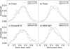 |
Fig. B.3. Histograms of the semi-axis ratios of thermal flare X-ray sources of various C–X-class flares observed with RHESSI (Warmuth & Mann 2013). The semi-axes were calculated from 2D elliptical Gaussian fits to RHESSI images calculated with four image reconstruction algorithms: clean (a), pixon (b), visibility forward fit (single elliptical Gaussian), and MEM-NJIT (d). 1D Gaussian fits to the CDFs of these distributions are shown in orange. The mean and standard deviation of the fits are shown in the legend of each panel. |
Based on the above distributions of ϕ and ρ, Figure B.4 shows the cumulative distribution functions (CDFs) of the orientation area scaling factor for several observer separations, θ. The CDFs are not symmetric or even peaked. This shows that the mean is not necessarily a good representation of the distribution. A better representation may be the value at which the “true” orientation area scaling factor (i.e. the one that retrieves the true source area) is equally likely to be larger or smaller. This is given by the x-value corresponding to CDF = 0.5, shown by the middle dashed horizontal line in Figure B.4, and as a function of θ by the solid line in Figure B.5a. We can now estimate the area scaling factor, κ, and hence the source area A0, by multiplying the representative orientation area scaling factor at the relevant observer separation angle by sin2θ. This is shown as a function of observer separation by the solid line in Figure B.5b.
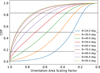 |
Fig. B.4. CDF of the orientation area scaling factor (Equation B.5) assuming that the source orientation, ϕ, is drawn from uniform distributions in the range 0 ° ≤ ϕ < 180° and the semi-axis ratios, ρ, from the Gaussian distribution in Figure B.3c. The CDF is shown for several values of observer separation angle, θ. The horizontal dashed lines trace the area scaling factor values at CDF = 0.1667, 0.5, 0.8333. The area scaling factor that recovers the true source area is twice as likely to lie within the upper and lower dashed lines as outside them. The dashed green-yellow line at θ = 95.4° represents the relation for the STIX-XRT-source separation angle for the SOL2021-05-07T18:43 M3.9 flare. |
B.4. Uncertainties of the corrected cross-section area
Defining the geometrical uncertainty of the estimated cross-section area (and hence the derived source volume) is equivalent to defining the uncertainty of the area scaling factor. However, the area scaling factor as a function of θ is not peaked, symmetric, or Gaussian, and so the standard deviation may not be a meaningful representation of its dispersion. An alternative measure of the uncertainty is the central range, which is twice as likely to include the true scaling factor as to exclude it, that is, the range defined by the x-values corresponding to 0.1667 < CDF < 0.8333. This is analogous to a ±σ uncertainty for a Gaussian distribution. The uncertainty range defined in this way is shown as a function of θ by the dashed lines in Figure B.5a and the corresponding uncertainties on κ by the dashed lines in Figure B.5b. When a higher threshold of certainty is desired, the same technique can be used to define the uncertainty range to be three, four, or more times more likely to include the true area scaling factor as to exclude it. In this study, we use an uncertainty threshold of a factor of 2.
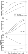 |
Fig. B.5. a) Orientation area scaling factor, κθϕρ, as a function of observer separation angle, θ, taken from its CDF (Figure B.4). The solid line is the relation at CDF = 0.5. This level is equally likely to be greater or lower than the true scaling factor, i.e. the one that recovers the true source area or volume. The dashed lines correspond to CDF = 0.1667, 0.8333 and represent the central range that is twice as likely to include the true scaling factor. b) Area scaling factor, κ. Equivalent to panel a, multiplied by sin2θ. c) Fractional uncertainty range of the area scaling factor (dashed lines). The vertical dotted line represents the observer separation angle from the X-ray source of the SOL2021-05-07T18:43 M3.9 flare (95.4°), equivalent to 84.6° due to symmetry about 90°. |
Figure B.5c shows the uncertainty interval on the area scaling factor in Figure B.5b (dashed lines) normalised by the representative area scaling factor (solid line) as a function of observer separation angle, θ. The smallest uncertainty range, and hence the optimal observer separation angle, is at 90°. However, uncertainties remain minimal in the range 90° ± 5° and are still relatively small in the range 90° ± 20°. Beyond this, the uncertainties grow significantly. However, 3D reconstruction can still be performed provided the larger uncertainties are acceptable for the science case.
Finally, we should note two things. Firstly, the above derivations rely on the assumption that the true source cross-sections are elliptical, or that they at least have a symmetry that is similar to that of an ellipse. Secondly, the above method does not provide better estimates of the source boundaries and so does not help in a comparison to the position of other features, such as EUV flare loops. However, the derived centre of the source is not affected by the observer separation angle or source orientation. Therefore, as long as the source symmetry is similar to that of an ellipse, the spatial relation between the central axis of the X-ray source and other features can be made quite faithfully.
B.5. Derivation of Equation B.4
Consider the case of the solid ellipse in Figure B.1 centred on the origin with a semi-major axis, a, a semi-minor axis b, and an angle ϕ between its semi-major axis and the x-axis. As previously stated, we call this “the source”. The source is bounded by a parallelogram with an acute angle of θ whose horizontal sides are parallel to the x-axis. The dashed ellipse is the maximum-area ellipse that can be inscribed in the parallelogram. Again, as previously stated, we call this “the derived ellipse”, and denote its semi-major and semi-minor axes as a′ and b′, respectively. To derive Equation B.4, we first recognise that the ratio of the derived area (Aθϕρ) to the source area (A0) (i.e. the area scaling factor, κ) is
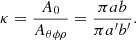
Next, we recall that two diameters of an ellipse are conjugate if and only if the line tangent to the ellipse at the end of one diameter is parallel to the other diameter. We furthermore recall that a maximum-area ellipse inscribed in a parallelogram is always tangent to the parallelogram at the midpoints of its sides. Therefore, the line segments joining opposite tangent points are conjugate diameters. Now we recall that the product of the conjugate diameters, d1 and d2, is related to the product of the ellipse semi-axes by
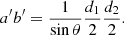
Therefore, Equation B.6 can be rewritten as
Finally, we recognise that the lengths of the above conjugate diameters are the same as the sides of the parallelogram. Therefore, the strategy is to derive the lengths of the sides of the parallelogram as a function of the source semi-axes, a and b, the source orientation angle, ϕ, and the parallelogram (observer separation) angle, θ, and plug them into Equation B.8.
First, we derive the equations of the lines defining the parallelogram. Their slopes are by definition 0 and tanθ. Therefore, the intercepts alone remain to be found. We start with the sides parallel to the x-axis. The equations of their lines are of the form

The equation of the source ellipse is
For arithmetic simplicity, this can be re-expressed as
where μ = 1/tanϕ. We substitute Equation B.9 into Equation B.11. Expanding the terms and rearranging them gives

This is a quadratic equation in x, for which the solution is
where α = (b2μ2 + a2), β = 2μc1(b2 − a2), and γ = (b2 + μ2a2) − a2b2/sin2ϕ. However, we know the lines are tangent to the ellipse. Therefore, there is only one solution for x, which requires that β2 − 4αγ = 0. Substituting for α, β, and γ, and expanding and rearranging gives
Merging the two terms in the denominator and recalling that μ = 1/tanϕ enables us to re-express it as μ2 + 1. The above equation can hence be rewritten as
Multiplying above and below  by sin2ϕ reveals that it equals sin2ϕ, while multiplying above and below
  by cos2ϕ reveals that it equals cos2ϕ. Hence,
where the two solutions correspond to the upper and lower sides of the parallelogram.
The length of the diagonal sides of the parallelogram are given by the perpendicular distance between the two horizontal tangents (dotted orange line, Figure B.1) divided by sin θ, that is,

For later convenience, we re-express this as
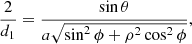
where ρ = b/a is the ratio of the semi-minor to semi-major axes.
The same strategy is used to find the length of the other sides of the parallelogram, d2. The equations of these lines have the form

where m = tanθ. Substituting Equation B.19 into Equation B.11, expanding, and rearranging gives

where η = μ + m and ε = 1 − μm. Once again, this is a quadratic equation of the same form as Equation B.13, where this time α = (b2η2 + a2ε2), β = 2c(b2η − a2με), and γ = c2(b2 + a2μ2)−a2b2/sin2θ. Once again, we use the fact that there is only one solution for x for tangents, and hence, β2 − 4αγ = 0. Substituting for α, β, and γ, expanding, and rearranging gives
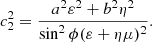
Expanding and merging the terms of the denominator and recalling that ε = 1 − μm, η = μ − m, and μ = 1/tanθ reveals that it can be re-expressed simply as μ2 + 1, which is equivalent to 1/sin2θ. Hence, the above equation can be rewritten as

Re-expressing the factors in brackets in terms of ϕ, recalling that m = tanθ, and taking the square root of both sides gives

Once again, the two solutions correspond to the two slanted sides of the parallelogram.
The length of the horizontal sides of the parallelogram is given by the horizontal distance between the lines defined by c2. This is equivalent to the distance between the points at which the lines cross the x-axis, that is, 2|c2|/m. Dividing Equation B.23 by m, and recalling that m = tanθ gives
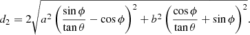
Once again, re-expressing for subsequent convenience gives
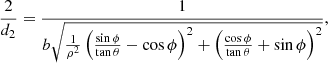
where ρ = b/a is the ratio of the semi-axes, as before.
Finally, combining Equations B.8, B.18 and B.25 gives Equation B.4,
![$$ \begin{aligned} \kappa = \frac{A_0}{A_{\theta \phi \rho }} = \frac{\sin ^2\theta }{\sqrt{(\sin ^2\phi + \rho ^2 \cos ^2\phi ) \left[ \frac{1}{\rho ^2} \left( \frac{\sin \phi }{\tan \theta } - \cos \phi \right)^2 + \left( \frac{\cos \phi }{\tan \theta } + \sin \phi \right)^2 \right]}} \end{aligned} $$](/articles/aa/full_html/2024/01/aa47212-23/aa47212-23-eq52.gif)
All Tables
Spatial resolution of XRT compared to that of STIX at different distances from Sun centre.
All Figures
|
Fig. 1. Summary of observations of the SOL2021-05-07T18:43 M3.9 flare. a) Positions of XRT, STIX and the flare (not to scale) as seen from the ecliptic north pole. b) and c) Full-disk views of the Sun in the AIA 1600 Å channel as seen from the positions of STIX and XRT. The orange boxes highlight the flaring active region (NOAA AR 12822). d) Light curves of the flare X-ray emission as measured in the GOES/XRS 1–8 Å channel (black), STIX 22–50 keV (blue) and 6–10 keV (red) bands, and the XRT Be-thick filter (orange). The dashed vertical lines show the interval for which 3D reconstruction was performed. Due to the different light-travel times from the active region to the two spacecraft, the times in this figure have been transformed to light-departure time, i.e. the time at which the emission left the active region. e) and f) Images of the thermal flare loop-top source (red contours) taken by STIX (panel e, 6–10 keV) and XRT (panel f, Be-thick filter), overlaid on AIA 1600 Å observations of the flare ribbons. The non-thermal footpoints imaged by STIX (blue contours, 22–50 keV) are also shown in panel e. |
| In the text | |
|
Fig. 2. 3D reconstruction via elliptical tie-pointing, adapted from Fig. 2 of Inhester (2006) and Byrne et al. (2010). a) Epipolar planes (blue rectangles) cutting through an X-ray source (elliptical orange spheroid) at progressively steepening angles. By definition, all planes pass through the epipole (dashed line) joining observers 1 (green circle) and 2 (purple circle). b) and c) 2D images of the X-ray source (orange ellipse) as seen by observers 1 and 2, respectively. The different sizes and orientations of the source are due to the source asymmetry and the different viewing angles of the observers. The blue lines show the projections of the epipolar planes onto the images. They converge towards the epipole, but in the case of flare observations, they are effectively parallel because the flare sources are small relative to the source-observer distances. The green and purple points denote the intersections of the epipolar planes with the source boundary. d) Lines of sight tangent to the X-ray source as seen from observers 1 (green) and 2 (purple) in a single epipolar plane. The lines of sight are defined by the intersections of the plane and the source boundary in the images (green and purple points in panels b and c). They form a quadrilateral within which an ellipse is inscribed to represent a cross section of the source. e) Same as panel d, repeated for multiple epipolar planes. By stacking the cross sections (orange ellipses), the X-ray source can be reconstructed in 3D. |
| In the text | |
|
Fig. 3. Demonstration of how XRT is used to constrain the source boundary threshold as seen by STIX. a) XRT Be-thick image showing the source boundary (blue contour; Eq. (2)) and the epipolar planes that bound it (green). b) Corresponding 6–10 keV STIX image with three source contours (inner dashed red line: 50%; solid red line: 37%, outer dashed red line: 30%) and the same epipolar planes as in panel a (green) projected to the STIX viewing angle. Only one contour (solid red) is tangent to both bounding epipolar planes and so represents the source boundary as seen by STIX. |
| In the text | |
|
Fig. 4. 3D reconstructions created with the observations shown in Figs. 1e,f and visualised using JHelioviewer. The thermal X-ray loop-top source of the flare (stacked red ellipses) is seen from three different viewing angles. Panels c and d show the same viewing angle and field of view. The thermal X-ray source is overlaid on a reprojected AIA 1600 Å image (green, panels a–c) and HMI magnetogram (black/white, panel d). Panels a–c also show elliptical forward-fit STIX images of the non-thermal flare footpoints (blue) as seen in 22–50 keV. The orange line in all panels is a semi-ellipse drawn between the footpoints through the centre of the thermal source as an approximation of the flare loops. The X-ray footpoint sources are omitted from panel d to give a clearer view of the magnetogram, but their locations can be inferred from the ends of the orange loop. For reference, the green and red lines show the heliocentric Stonyhurst lines of latitude and longitude, and each panel shows the north-west axes in its corners. |
| In the text | |
|
Fig. 5. a) Temporal evolution of the X-ray loop-top source volume of the SOL2021-05-07T18:43 M3.9 flare. The 3D-derived volume (solid black curve) is compared to those derived from the traditional area-to-volume scaling law (Eq. (1)) based on the STIX 6–10 keV (blue curve) and XRT Be-thick (gold curve) images. The dotted black curves show the range within which the true source volume is twice as likely to lie based on the geometric uncertainties of the 3D reconstruction method. b) STIX- (blue curve) and XRT-area-scaled volumes (gold curve) normalised by the 3D-derived volume. The dotted lines show the area-scaled volumes normalised by the 3D volume uncertainty range. |
| In the text | |
|
Fig. 6. Temporal evolution of the thermal X-ray loop-top source of the SOL2021-05-07T18:43 M3.9 flare. a)–d) Source height, volume, and STIX-derived temperature and emission measure. The dotted lines in panel b have the same meaning as in Fig. 5a. The error bars in panels c,d represent the fitting uncertainties to the STIX spectra. e)–h) Source-averaged electron number density, mass, gravitational potential energy, and electron thermal energy derived from panels a–d. The dotted lines represent the uncertainty due to volume alone, and the error bars denote the combined volume and spectral fit uncertainties. |
| In the text | |
|
Fig. A.1. Normalised temperature response functions for the STIX 6 – 10 keV band (solid blue) and the highest-energy XRT filters: Be-thick (solid orange), Al-thick (dashed green), and Be-thin (dotted red). The Be-thick filter overlaps most with the STIX 6 – 10 keV response. |
| In the text | |
|
Fig. A.2. a) X-ray image of a C4 flare that peaked at 2021-11-01 23:39 UT as observed at Earth. The red and black show the XRT Be-thick filter image, and the white lines show 30%–90% contours of the STIX 6 – 10 keV emission. The STIX image was produced by forward-fitting an elliptical Gaussian, and its size has been corrected for the difference in observer distance. Despite the different temperature responses and imaging techniques of the two instruments, the source areas agree very well. b) Light curves of the STIX 6 – 10 keV (solid blue) and XRT Be-thick (dashed orange) emission. The source size in panel a) agrees despite a slightly different evolution of the light curves. |
| In the text | |
|
Fig. B.1. Difference between the true cross-sectional geometry of a source (solid ellipse) and the maximum-area (dashed) ellipse derived from observations taken by two observers separated by an angle θ. The source has semi-major and semi-minor axes a and b, and an orientation angle, ϕ, between its semi-major axis and the lines of sight of observer 1. The derived ellipse has conjugate diameters, d1 and d2, with the same lengths as the parallel sides of the bounding parallelogram (solid lines) formed by the tangential lines of sight (dotted lines). The solid blue line represents the x-axis, and the dotted orange line represents the distance, 2c1, between the lines of sight from observer 1. |
| In the text | |
|
Fig. B.2. Area scaling factor (Equation B.5) as a function of source orientation, ϕ, and observer separation angle, θ, for two source semi-axis ratios, ρ = 0.5 (a) and ρ = 0.25 (b). The closer ρ is to 1 and the closer θ is to 90° the smaller the scaling factor, i.e. the closer the derived area is to the source area. The dashed green-yellow curves at 95.4° represent the separation angle of STIX and XRT relative to the flare X-ray source of SOL2021-05-07T18:43 M3.9. |
| In the text | |
|
Fig. B.3. Histograms of the semi-axis ratios of thermal flare X-ray sources of various C–X-class flares observed with RHESSI (Warmuth & Mann 2013). The semi-axes were calculated from 2D elliptical Gaussian fits to RHESSI images calculated with four image reconstruction algorithms: clean (a), pixon (b), visibility forward fit (single elliptical Gaussian), and MEM-NJIT (d). 1D Gaussian fits to the CDFs of these distributions are shown in orange. The mean and standard deviation of the fits are shown in the legend of each panel. |
| In the text | |
|
Fig. B.4. CDF of the orientation area scaling factor (Equation B.5) assuming that the source orientation, ϕ, is drawn from uniform distributions in the range 0 ° ≤ ϕ < 180° and the semi-axis ratios, ρ, from the Gaussian distribution in Figure B.3c. The CDF is shown for several values of observer separation angle, θ. The horizontal dashed lines trace the area scaling factor values at CDF = 0.1667, 0.5, 0.8333. The area scaling factor that recovers the true source area is twice as likely to lie within the upper and lower dashed lines as outside them. The dashed green-yellow line at θ = 95.4° represents the relation for the STIX-XRT-source separation angle for the SOL2021-05-07T18:43 M3.9 flare. |
| In the text | |
|
Fig. B.5. a) Orientation area scaling factor, κθϕρ, as a function of observer separation angle, θ, taken from its CDF (Figure B.4). The solid line is the relation at CDF = 0.5. This level is equally likely to be greater or lower than the true scaling factor, i.e. the one that recovers the true source area or volume. The dashed lines correspond to CDF = 0.1667, 0.8333 and represent the central range that is twice as likely to include the true scaling factor. b) Area scaling factor, κ. Equivalent to panel a, multiplied by sin2θ. c) Fractional uncertainty range of the area scaling factor (dashed lines). The vertical dotted line represents the observer separation angle from the X-ray source of the SOL2021-05-07T18:43 M3.9 flare (95.4°), equivalent to 84.6° due to symmetry about 90°. |
| In the text | |
Current usage metrics show cumulative count of Article Views (full-text article views including HTML views, PDF and ePub downloads, according to the available data) and Abstracts Views on Vision4Press platform.
Data correspond to usage on the plateform after 2015. The current usage metrics is available 48-96 hours after online publication and is updated daily on week days.
Initial download of the metrics may take a while.