| Issue |
A&A
Volume 681, January 2024
|
|
|---|---|---|
| Article Number | A111 | |
| Number of page(s) | 12 | |
| Section | Interstellar and circumstellar matter | |
| DOI | https://doi.org/10.1051/0004-6361/202346423 | |
| Published online | 25 January 2024 | |
Reconstructing Galactic magnetic fields from local measurements for backtracking ultra-high-energy cosmic rays
1
Department of Physics & ITCP, University of Crete,
70013
Heraklion,
Greece
e-mail: This email address is being protected from spambots. You need JavaScript enabled to view it.
2
Institute of Astrophysics, Foundation for Research and Technology-Hellas,
Vasilika Vouton,
70013
Heraklion,
Greece
3
Ludwig Maximilian University of Munich,
Geschwister-Scholl-Platz 1,
80539
Munich,
Germany
4
Max Planck Institute for Astrophysics,
Karl-Schwarzschild-Straße 1,
85748
Garching,
Germany
Received:
15
March
2023
Accepted:
14
October
2023
Abstract
Context. Ultra-high-energy cosmic rays (UHECRs) are highly energetic charged particles with energies exceeding 1018 eV. These energies are far greater than those achieved in Earth-bound accelerators, and identifying their sources and production mechanism can shed light on many open questions in both astrophysics and high-energy physics. However, due to the presence of the Galactic magnetic field (GMF) they are deflected, and hence the location of their true source on the plane of the sky (PoS) is concealed. The identification of UHECR sources is an open question, excacerbated by the large uncertainties in our current understanding of the three-dimensional structure of the GMF. This difficulty arises from the fact that currently all GMF observations are integrated along the line of sight (LoS). However, thanks to upcoming stellar optopolarimetric surveys as well as Gaia data on stellar parallaxes, we expect that local measurements of the GMF in the near future will become available.
Aims. Given such a set of (sparse) local GMF measurements, the question is how to optimally use them in backtracking UHECRs through the Galaxy. In this paper, we evaluate the reconstruction of the GMF, in a limited region of the Galaxy, through Bayesian inference, using principles of information field theory.
Methods. We employed methods of Bayesian statistical inference in order to estimate the posterior distribution of the GMF configuration within a certain region of the Galaxy from a set of sparse simulated local measurements. Given the energy, charge, and arrival direction of a UHECR, we could backtrack it through GMF configurations drawn from the posterior, and hence calculate the probability distribution of the true arrival directions on the PoS, by solving the equations of motion in each case.
Results. We show that, for a weakly turbulent GMF, it is possible to correct for its effect on the observed arrival direction of UHECRs to within ~3°. For completely turbulent fields, we show that our procedure can still be used to significantly improve our knowledge on the true arrival direction of UHECRs.
Key words: magnetic fields / (ISM:) cosmic rays / turbulence
© The Authors 2024
 Open Access article, published by EDP Sciences, under the terms of the Creative Commons Attribution License (https://creativecommons.org/licenses/by/4.0), which permits unrestricted use, distribution, and reproduction in any medium, provided the original work is properly cited.
This article is published in open access under the Subscribe to Open model. This email address is being protected from spambots. You need JavaScript enabled to view it. to support open access publication.
1 Introduction
The identification of ultra-high-energy cosmic ray (UHECR) sources remains one of the central questions in modern high-energy astrophysics. A possible resolution to this problem would shed light on the astrophysical mechanism that produces UHECRs, as well as their composition (either protons or heavier nuclei), which at high energies still remains a subject of debate. Knowledge of their composition may, in turn, provide insights into high-energy particle phenomenology at energies not yet probed by particle accelerators (Pavlidou & Tomaras 2019; Romanopoulos et al. 2022a,b).
Despite the fact that several theoretical candidates for UHECR sources have been proposed (Bhattacharjee & Sigl 2000; Torres & Anchordoqui 2004), the identity of their sources remains elusive. The primary reason for this is that UHECRs are charged particles and are hence deflected by the Galactic magnetic field (GMF) as well as the intergalactic magnetic field. Even if several of the detected UHECRs originate from a single bright, nearby cosmic ray source di Matteo et al. (2023), their arrival directions would be very spread out in the sky, and any residual clustering would be centered off-source, due to magnetic deflections. This is unlike the case of photons or neutrinos, in which positional identifications events with their likely sources can be attempted even with very low-number statistics.
The main difficulty in resolving the GMF stems from the fact that 3D tomographic realizations of the intervening magnetic fields are notoriously difficult to acquire. Specifically for the GMF, most observables that are currently available are integrated along the line of sight (LoS). Due to this limitation, and specifically for the GMF, the principal approach (Takami & Sato 2010) is relying on GMF models that are acquired by parameter-fitting three separate components − a toroidal, a poloidal, and a Gaussian random field (Jansson & Farrar 2012a,b; Sun et al. 2008; Sun & Reich 2010).
Nonetheless, it is possible to acquire direct information regarding the 3D structure of the GMF. Gaia data on stellar distances have localized more than a billion stars in the Galaxy by accurately determining stellar parallaxes (Gaia Collaboration 2016, 2021; Bailer-Jones et al. 2021). This data − in addition to other available spectroscopic data − has been used in order to construct 3D tomographic maps of the dust density distribution of certain Galactic regions (Green et al. 2019; Lallement et al. 2019; Leike & Enßlin 2019). These reconstructions, however, do not constrain the magnetic field that is of primary interest in cosmic ray physics.
Nonetheless, there do exist probes that provide information regarding the structure of the GMF in 3D. For instance, the linear polarization of starlight is of particular interest; while starlight starts off unpolarized from its source, it will usually acquire a linear polarization until it is observed on Earth, due to dichroic absorption by dust particles aligned with the ambient magnetic field (Andersson et al. 2015).
Upcoming optopolarimetric surveys, such as PASIPHAE (Tassis et al. 2018; Maharana et al. 2021, 2022; Magalhães 2012), are expected to provide a large number of high-quality stellar polarization measurements on more than a million stars. With stellar distances also known from the Gaia survey, this data can be used to provide direct tomographic measurements of the plane of the sky (PoS) component of the GMF at the location of the dust clouds (Panopoulou et al. 2017; Pelgrims et al. 2023; Davis 1951; Chandrasekhar & Fermi 1953; Skalidis et al. 2021). Used jointly with available LoS information (see for example Tahani et al. 2022a,b), we can expect to have local and sparse data of the GMF in the near future, which could be used in order to provide a 3D tomographic map of a particular region of interest. Given such a map, one can then backtrack UHECRs through that region, thus improving the localisation of their source on the sky, modulo the effects of the intergalactic magnetic field. To be more specific, one might be interested in reconstructing the region of the GMF through which the UHECRs “hotspots” (Kawata et al. 2019; Abbasi et al. 2014; Pierre Auger Collaboration 2017) have to travel.
In this paper, we address the problem of reconstructing the posterior density function (PDF) for the true arrival directions of UHECRs, using local, sparse, and (statistically) uniformly distributed GMF measurements. In essence, we are interested in solving the inverse problem in a Bayesian setting, wherein one is given local data and tasked with calculating the posterior distribution of the GMF configurations in the region of interest. For Bayesian field inference, information field theory (IFT) was developed Enßlin et al. (2009), and demonstrated in a number of contexts Enßlin (2022). Here, we use an adapted version of the algorithm used in Leike & Enßlin (2019), after generalising it in order to make it applicable to divergence-free vector fields. Using the reconstructed posterior distribution over GMF realizations, we correct for the effect of the GMF on the observed arrival direction of the UHECR.
The work is structured as follows: in Sect. 2, we describe the Bayesian setting that is employed, and set out the principal components of the algorithm that forms the core of our reconstruction scheme, as well as describe our assumptions. In Sect. 3, we present the main results of this paper, by applying our reconstruction scheme to magnetic fields that are locally and sparsely sampled, for different relative strengths of the turbulent and the uniform component, as well as different sampling intervals. In Sect. 4, we summarize and discuss our conclusions.
2 Methodology
In Bayesian inference for continuous signals, we are in general interested in reconstructing the posterior probability distribution, φ(x), defined over a domain, 𝒱, from a given data set, d:
 (1)
(1)
The distribution, P(d|φ), is the likelihood, and quantifies how likely acquiring d as our data is, given that the configuration is φ(x). The function, P(φ), is the prior probability density, containing our information on φ(x) before d is taken into account. The proportionality factor in Eq. (1) is determined by normalising the posterior to unity.
Mathematically, φ(x) is a continuous function, and the distributions P(φ), P(φ|d), and P(d|φ) are functionals. For example, an important case is the Gaussian distribution,
![Mathematical equation: ${\cal G}(\varphi - m,\Phi ) \equiv {{\exp \left[ { - {1 \over 2}(\varphi - m){\Phi ^{ - 1}}(\varphi - m)} \right]} \over {|2\pi \Phi {|^{{1 \over 2}}}}}$](/articles/aa/full_html/2024/01/aa46423-23/aa46423-23-eq2.png) (2)
(2)
where m(x) = 〈φ(x)〉 is the mean. The quantity Φ(x1, x2) = 〈δφ(x1)δφ(x1)〉 is the covariance of the distribution, where we have defined δφ(x) ≡ φ(x) − m(x). |Φ| denotes the determinant of Φ. In Eq. (2), there is also an implicit integration, that is,
![Mathematical equation: $\eqalign{ & (\varphi - m){\Phi ^{ - 1}}(\varphi - m) \equiv \cr & \,\,\,\,\,\,\,\,\,\,\,\,\,\,\,\,\,\,\,\,\,\,\quad \int {{{\rm{d}}^3}} x{{\rm{d}}^3}x'[\varphi ({\bf{x}}) - m({\bf{x}})]{\Phi ^{ - 1}}\left( {{\bf{x}},{\bf{x'}}} \right)\left[ {\varphi \left( {{\bf{x'}}} \right) - m\left( {{\bf{x'}}} \right)} \right]. \cr}$](/articles/aa/full_html/2024/01/aa46423-23/aa46423-23-eq3.png)
In order to avoid cluttered notation, this integration will always be written implicitly.
2.1 Prior
The signal that we are interested in reconstructing is the GMF, B(x), which is a vector quantity. Following Eq. (2), the prior is written as
![Mathematical equation: ${\cal G}(\delta {\bf{B}}({\bf{x}}),M) \equiv {{\exp \left[ { - {1 \over 2}\delta {B_i}M_{ij}^{ - 1}\delta {B_j}} \right]} \over {|2\pi M{|^{{1 \over 2}}}}},$](/articles/aa/full_html/2024/01/aa46423-23/aa46423-23-eq4.png) (3)
(3)
where δBi(x) = Bi(x) − 〈Bi(x)〉, with 〈Bi(x)〉 denoting the mean of the distribution.
Here the indices correspond to individual components of the vector B(x), and the Einstein summation convention is assumed, and B0 is the mean field. Here, the covariance matrix inherits two indices, since by definition
 (4)
(4)
In the absence of information regarding the geometry and statistics of the GMF in the region of interest, we modeled the prior as being statistically isotropic and homogeneous. In Fourier space, this is equivalent to assuming that the two-point correlation function Eq. (4) takes the form
 (5)
(5)
where
 (6)
(6)
is the transverse projection operator,  denotes the unit k-vector in the ith direction, δij is the kronecker delta, δ(3)(k − k′) is the three dimensional Dirac delta function, and
  denotes the complex conjugate of
  . Furthermore, the norm of the k-vector is henceforth denoted as k. The function, P(k), is the magnetic power spectrum, and needs to be inferred as well. Equation (5) assumes that no prior expectation of the presence of the helicity of any sign exists1. We note that magnetic helicity in the reconstructed magnetic field is not thereby excluded, but just needs to be requested by the data and will not be enforced by the prior.
Instead of inferring B(x) directly, it is more practical to work with a latent vector field, φ(x), that does not satisfy the divergence free condition and that thus contains more degrees of freedom than needed. The Fourier space correlation structure for φ will be assumed to be isotropic and homogeneous, and this will take the form
 (7)
(7)
with the understanding that B(x) and φ(x) are related to each other by an application of Ƥij(k) by
![Mathematical equation: ${\hat B_i}({\bf{k}}) \equiv {3 \over 2}{{\cal P}_{ij}}({\bf{k}}){\hat \varphi _j}({\bf{k}}) = {3 \over 2}\left( {{{\hat \varphi }_i}({\bf{k}}) - \left[ {{{\hat \varphi }_j}({\bf{k}}){k_j}} \right]{{{k_i}} \over {{k^2}}}} \right),$](/articles/aa/full_html/2024/01/aa46423-23/aa46423-23-eq13.png) (8)
(8)
in Fourier space. Are these three words − “in Fourier space” − connected to the previous equation, or are they not supposed to be here? This definition is such that the resulting field, B, is guaranteed to be divergence-free, since then  in harmonic space, implying that ∇ • B = 0 as required. The 3/2 factor compensates for the loss of power that the subtraction of degrees of freedom causes. This is justified by the original a priori assumption of statistical isotropy for φ, which leads to equipartition along the three directions in Fourier space. Equation (8) is in accordance with the correlation structure assumed in Eq. (5) (Jaffe et al. 2012).
The power spectrum, P(k), is unknown and needs to be inferred as well. It is modeled as the sum of a power law component and an integrated Wiener process component (for details regarding the generative model for power spectra, the reader should refer to Arras et al. 2022). The parameters that define it, as well as their respective prior PDFs, are:
- 1.
The total field offset for all field components. This controls the mean value around which the random field fluctuates, B0. We set a value of 0, which means that in the absence of data the mean overall field is assumed to be zero-centered.
- 2.
The standard deviation of the total offset. This is a random variable with a prior log-normal distribution. We set its mean at 3 μG and its own standard deviation at 1 μG. This reflects our current understanding of typical GMF values in the interstellar medium that a (randomly oriented) mean magnetic field of this typical strength within the reconstructed volume is conceivable, but not enforced.
- 3.
The total spectral energy2. This controls the amplitude of the fluctuations in configuration space. Its prior probability distribution is log-normal, with a mean and standard deviation set to unity. This is essentially the standard deviation of the field values calculated over the complete set of voxels.
- 4.
The spectral index; the exponent of the pure power law component. Its prior distribution is normal, with a mean set as the Kolmogorov index, −11/3, and we assumed a unit standard deviation.
- 5.
Amplitude of the integrated Wiener process component, controlling the deviations from a pure power law.
Its prior distribution is log-normal, with a mean and standard deviation equal to 1.5 and 1, respectively. These parameters were chosen so as to allow for deviations from a pure power law without destroying the approximately power-law overall behavior of the power spectrum. “Approximately power-law overall behavior” does not sound right. Do you mean power-law-like behavior perhaps? Please rephrase.
The parameters of the amplitude model were assumed to be relative to a unit-less power spectrum; in other words, the parameters were assumed to be agnostic with regard to changes in the volume of the target subdomain, 𝒱3. In Table 1, we summarise our choice for the probability distributions of the parameters of the power spectrum, as well as their respective means and standard deviations.
In closing the discussion on the prior, we consider the implementation of anisotropy. In general, the GMF in the region within which we wished to reconstruct it was assumed to admit the two-component structure
 (9)
(9)
where B0 is a uniform field parallel to the PoS. Since the observed arrival velocity of the UHECR was chosen to be parallel to the LoS (see Sect. 3), the PoS component of B0 dominates the UHECR’s deflection and the LoS component is hardly constrained. Additionally, b(x) is a fluctuating field with zero mean, which can be physically interpreted as the turbulent field. Our prior is agnostic to the direction and magnitude of B0, and inferring it from the data is a central task. The relative strength of the two components is quantified by the turbulent-to-uniform ratio, λ, defined as
 (10)
(10)
where B0 is the norm of B0, and brms is the root mean square value of the fluctuating component’s magnitude, in the domain 𝒱. For λ ≫ 1 we have strong turbulence, for λ ≫ 1 we have weak turbulence, and for λ ≃ 1 we have intermediate turbulence. As we will demonstrate, λ is the main parameter that controls how well the sources of UHECRs can be localized by the use of local GMF data along, of course, with the sampling rate.
Parameters that define the power spectrum prior.
2.2 Likelihood
In order to construct the likelihood, we considered how the data is acquired from the true signal, B. We assumed that the i-th data point is given by a measurement process of the form
 (11)
(11)
The operator, R, is a map from the signal space to the data space. For this proof of concept work, we made the simplifying assumption that local measurements of field components are possible, in other words R(x, xi) = δ(3)(x − xi). In practice, most astrophysi-cal measurements of magnetic fields (Faraday rotation, UHECR deflection, etc.) provide at least a LoS, particle trajectory, or even sub-volume averaged field strength. This only complicates the numerical reconstruction of fields, but does not imply conceptual changes in the formalism.
Thus, since we assumed local measurements, R was here assumed to be a mask operator. In practice, since the mock signal is discretized into voxels, R is simply a very sparse matrix. The full vector, d, is therefore a concantenation of a number of 3D vectors known on a finite number of points inside the domain wherever we have measurements, and undefined anywhere else. Simply put, then, the operator, R, merely acts a selection operator that picks out the values of B(x) where we have measurements. Physically, the assumption was that at the positions where GMF measurements can be obtained, all three components of B(x) can be measured. This can be accomplished, for example, by Zeeman observations for the LoS component of the magnetic field. The PoS component of the magnetic field can be recovered through a combination of stellar optopolarimetry and stellar distance measures. Optopolarimetric measurements of stars of known distances can be decomposed to the contributions of individual clouds along the LoS Pelgrims et al. (2023). Then, the average direction of polarization angles induced on starlight by dichroic absorption due to a single cloud reveals the direction of the magnetic field in that cloud. The dispersion of these directions can yield a measurement (within a factor of two) of the magnetic field strength in the same cloud (Chandrasekhar & Fermi 1953; Davis 1951; Skalidis et al. 2021; Skalidis & Tassis 2021).
Additionally, the vector, n(i), was random noise added to the i-th noiseless data point. It was assumed to be drawn from a Gaussian distribution with a standard deviation equal to half the root-mean-square magnitude of the mock signal field. Physically, n(i) represents the measurement error, assuming an average signal-to-noise ratio S/N of two.
The likelihood was then calculated by marginalizing over the noise:
 (12)
(12)
where N is the noise covariance, and where we used the shorthand notation RB = ∫ R(x, xi)B(x)d3x. We can write the likelihood in terms of φ by absorbing Ƥij into R, that is, R′ ≡ RƤij.
Then, the likelihood becomes
 (13)
(13)
2.3 Approaching the posterior: Geometric variational inference
In the previous two sections, we described how we modeled the prior and the likelihood for our inference setting. From Eq. (1), the posterior is proportional to the product of the two.
Due to the fact that the magnetic power spectrum, P(k), needs to be inferred along with the configuration of the GMF, this inference problem is nonlinear. A way to see this is that the magnetic field, B(x), couples to P(k) through Eqs. (3) and (5). Moreover, the prior PDFs for the parameters that determine P(k) are not Gaussian (with the exception of the spectral index), which is an additional source of nonlinearity. Furthermore, there is no small parameter that could be used in a perturbative analysis about a linear inference case. For this reason, a non-perturbative scheme, called geometrical variational inference (geoVI) developed by Frank et al. (2021) was utilized. In this section we motivate the basic premises of geoVI.
The idea is to approximate the true posterior, P, with an approximate one, Q. The approximate posterior, Q, is chosen such that the Kullback-Leibler divergence (Kullback & Leibler 1951),
 (14)
(14)
between the actual posterior, P, and an approximate posterior, Q, is minimized. The main idea of geoVI is to achieve this minimization in a new coordinate system, chosen such that P − in the new coordinate system − locally closely resembles a normalized standard distribution. Once this is done, the approximating posterior, Q, is chosen to be of the form (3). Then, the mean and covariance are chosen as the parameters with respect to which the KL divergence is minimized.
A few more details on geoVI can be found in Appendix A and in Frank et al. (2021). Essentially, the algorithm provides approximate posterior samples that can follow the non-Gaussian structure of the posterior to a certain degree. geoVI can be invoked by the numerical information field theory (NIFTy) package in Python (Selig et al. 2013; Steininger et al. 2019; Arras et al. 2019). The input that is required is the likelihood and the prior of the original physical model, as described in Sects. 2.2 and 2.1, respectively.
3 Results
3.1 General procedure
We were now ready to construct a number of representative examples, in which we applied the procedure described in the previous section in order to reconstruct various assumed GMF geometries from a set of local, sparse, noisy, 3D GMF mock observations. All of the examples that we studied were created according to the following scheme:
We defined the domain: We chose a cube, 𝒱, of side length L = 3 kpc, with periodic boundary conditions (topologically a 3-torus), and evenly divided it into N3 voxels. The number, N, defines our resolution.
We produced a power spectrum, P(k), by randomly sampling each of its defining parameters from its respective distribution (see Sect. 2.1).
We produced the latent field, φ, with a correlation structure dictated by Eq. (7), with it taking a constant value over each voxel.
-
We created the fluctuating part of the synthetic signal in Fourier space, by acting on φ with the transverse projection operator;

After transforming into configuration space and computing the RMS value of the field, brms, we added the uniform component that lies along the x − y plane (serving as our PoS) of a magnitude λ−1 brms, for a desired value of λ. We rescaled the total field such that the total RMS magnitude is 5 μG.
-
We acted on the mock signal with a mask operator, which uniformly chooses a specified small fraction of voxels from the subdivided domain. This was done as follows: if Nd was the (approximate) number of data points we wished to have, then we acted on the original array with an operator that masked each voxel with a probability of 1 − Nd/N. Roughly, then, the number of voxels that survived was Nd, by construction.
However, it is more useful to refer to the mean sampling ‘rate’; since by construction the distribution of data points is spatially homogeneous, the mean distance between the data points, as a function of Nd, is

The mean sampling rate is thus defined as
 (15)
(15)In physical reality, the data points will be located wherever HI clouds exist in the region under study, which are not positioned uniformly within 𝒱 , and so the sampling rate will vary with vertical distance from the Galactic plane. Furthermore, there are also nonlocal measurements that, for example, average over a LoS. In future work, we shall also consider such effects.
-
We added noise: To each data vector created in the previous step, we added a random vector sampled from a multivariate Gaussian distribution meant to represent observational error. The variance of the distribution is
 (16)
(16)where Brms is the RMS value of the total magnetic field’s norm within 𝒱 , which is set to 5 μG (see step 4). The denominator on the right-hand side is chosen such that the average S/N is two.
We applied the geoVI algorithm to the data set (see Sect. 2.3). The output of the algorithm are samples of the posterior distribution.
An illustrative example is shown in Fig. 1, where we choose ksample = (600 pc)−1 as the mean sampling rate, and a turbulent-to-uniform ratio, λ = 0.2 (see Eq. (10)). In this case, the posterior mean essentially identifies the uniform component (Fig. 1c) provided the sparse and local data shown in Fig. 1b. The dominance of the ordered component results in a large scatter in the power spectrum (Fig. 2). To see why this is the case, we note that the zero mode of the field is
 (17)
(17)
Fig. 1 −
In the scenario of a strong uniform component, the modes  with k > 0 are poorly constrained by the data, which mainly inform with respect to the zero mode.
It is important to note, however, that the UHECR’s deflection is primarily influenced by the uniform component (or the zero mode), and is affected much less by the small-scale, turbulent fluctuations. Therefore, for the purposes of our inquiry, the recovery of the zero mode is enough to provide the leading order correction on the original arrival direction of UHECRs. In the next section, we apply the geoVI algorithm as exemplified in Fig. 1 specifically to the case of backtracking UHECRs back to their sources by utilising local data.
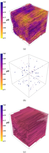 |
Fig. 1 Reconstruction of a 3D magnetic field within a cube of side L = 3 = kpc. Top: the ground truth; a uniform field parallel to the x − y plane with magnitude 5 μG, plus a turbulent, random, field with an RMS magnitude of 1 μG, corresponding to λ = 0.2 in Eq. (10). Middle: local data sampled randomly, with a constant mean sampling rate (600 pc)−1. The colormap is saturated at the maximum magnitude that appears in Fig. 1a. Bottom: the mean of the approximating posterior distribution attained via the geoVI algorithmn based on the data provided in Fig. 1b. |
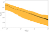 |
Fig. 2 The three-dimensional power spectrum, P3D(k), corresponding to the example showcased in Fig. 1. The black line is the power spectrum of the mock signal, while the orange envelope encompasses the posterior samples, providing the variance for the posterior mean power spectrum estimate. The wavevector, k, is given in units of 2π/N. The large scatter is due to the fact that we have few and noisy data points, in a signal that is dominated by its uniform component, and thus the modes with k > 0 are poorly constrained. |
3.2 Correcting the arrival directions of UHECRs
In the previous section, we demonstrated the results of the geoVI algorithm applied to sparse and local measurements of a magnetic field in the case of a strong uniform component. However, the quality of the reconstruction should be judged in context, as different degrees of resolution are required in different applications. In fact, in this context, the GMF reconstruction is a means to an end, the latter being correcting for the effect of the GMF on the arrival direction of the UHECRs, given their arrival direction and energy as observed on Earth.
Stated explicitly, the question is, given an observed arrival direction,  , of a charged particle of known lab-frame energy and charge, how to get the posterior distribution for its original, extragalactic direction, assuming we are provided with sparse and local measurements of the GMF within a region, 𝒱 , within which it traveled. Since the geoVI algorithm returns as output sample configurations of the GMF drawn from the posterior, we can reconstruct the UHECR’s path through each sample by solving the equations of motion backward (for details on how this is carried out in practice, see Appendix B). In the end, we are left with a distribution for possible paths, all converging to the velocity observed on Earth.
For the situation presented in Fig. 1, we considered a particle of charge e with final position, ri = (L/2, L/2,0)T (Earth’s location inside 𝒱), velocity direction,  in Galactic coordinates, and energy in the lab frame, E = 5 × 10¹⁹ eV, that was backtracked through the true GMF, as well as samples of the posterior distribution of the GMF given the local and sparse data shown in Fig. 1b. In Fig. 3, in Galactic coordinates, the observed arrival direction (black star), true arrival direction (red star), and posterior samples (dots in the viridis colormap), are shown. The colormap corresponds to the mean posterior distribution as inferred from our samples using the IFT-based density estimator, DENSe (Guardiani et al. 2022). The advantage of this method is that the parameters of the kernel are inferred instead of assumed, and the result of this algorithm are samples of possible distributions drawn from the posterior distribution of distributions, given the samples3. From the former, the mean is drawn as our estimate for the underlying distribution, shown in the colormap of Fig. 3.
It can be seen that we were able to substantially correct for the effect of the GMF. For the purpose of comparison, we also include the respective result obtained via two different, much simpler, reconstruction methods: 1) merely taking the vector mean of the data points (blue star), and 2) a nearest-neighbor estimate wherein one assumes that at each point in space the value of the GMF is that given by the nearest available data point (pink star). While all three of the methods are able to correct for the effect of the GMF by essentially picking out the zero mode − which in this case predominantly affects the UHECR paths − the IFT-based method is a statistically rigorous way to perform the inference, as it also provides a quantification of the inference’s uncertainty, a feature that the simpler methods lack. In addition, the simple methods assume either a low λ, or data points that are populated densely enough − something that cannot be expected from the distribution of dust clouds in real life applications.
In order to quantify the improvement in our knowledge, we used the Mahalanobis distance (Mahalanobis 1936) between a given arrival direction,  , and the posterior samples acquired from the geoVI algorithm,
![Mathematical equation: ${d_M}[\widehat {\bf{v}};P] = \sqrt {{{(\widehat {\bf{v}} - \hat \mu )}^T}{S^{ - 1}}(\widehat {\bf{v}} - \hat \mu )} ,$](/articles/aa/full_html/2024/01/aa46423-23/aa46423-23-eq30.png) (18)
(18)
where S−1 and  are the inverse covariance matrix and mean of
  , respectively. Essentially, dM measures how many standard deviations
  is located away from
  . If
. If  and
and  are the true and observed arrival directions, respectively shown in Figs. 1 and 3, we calculated that
 ![Mathematical equation: ${d_M}\left[ {{{\hat v}^{true}};P} \right] = 1.6\sigma $](/articles/aa/full_html/2024/01/aa46423-23/aa46423-23-eq37.png) and
and ![Mathematical equation: ${d_M}\left[ {{{\hat v}^{obs}};P} \right] = 22.8\sigma $](/articles/aa/full_html/2024/01/aa46423-23/aa46423-23-eq38.png) .
.
We also quantified our results using a different metric. Let  denote the arrival direction as obtained by backtracking through a reconstructed magnetic field. If we define the angle
 (19)
(19)
we are interested in the posterior mean of θ′, henceforth referred to as θ = 〈θ′〉.
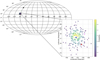 |
Fig. 3 Plane of the sky projections of the UHECR arrival directions as inferred given local and sparse GMF data based on 100 posterior samples (viridis colormap). The GMF reconstruction problem is the one shown in Fig. 1. The red star denotes the true arrival direction, while the black star denotes the observed arrival direction, and they are found 1.6σ and 22.8σ from the posterior’s mean, respectively. For comparison, we also inferred the UHECR arrival direction using a simple vector mean of all the GMF data points (blue star), as well as a a nearest-neighbor estimate (pink star), where at each point the GMF was assumed to be that dictated by the nearest available data point. These simple reconstruction methods do not provide an uncertainty quantification. In addition, they tacitly assume either a low λ, or data points that are populated densely enough – something that cannot be expected from the distribution of dust clouds in real life applications. |
3.3 Effect of the sampling rate
In order to see how local sampling of the GMF might help us resolve the UHECR initial directions in general, the same backtracking procedure that led to Fig. 3 was carried out for an ensemble of 100 GMF configurations, for three different values of the mean sampling rate; ksample = (300 pc)−1, (425 pc)−1, and (600 pc)−1, and each time a different field served as ground truth and was reconstructed, via the process described in Sect. 3.1. The angle, 6, defined at the end of the last section, was calculated in each case, and the histograms for each sampling rate considered are shown in blue, in Fig. 4. For reference, we also calculated the angle between  and the final velocity direction,
  ,
,
 (20)
(20)
The histogram for 60 is shown in red for each sampling rate considered. At zeroth order, without attempting to reconstruct the GMF at all, the UHECR’s path would not be altered, and so in this case  , trivially. Therefore, θ0 is the zeroth-order approximation, without any data points considered. As can be clearly seen, the usage of the local and sparse data, d, significantly corrects for the effect of the GMF on our knowledge of the UHECR arrival direction. Furthermore, as expected, increasing sampling rates tend to move the PDF for θ, P(θ), more toward θ = 0. In the extreme case of a perfectly known GMF, P(θ) would be a delta function centered on zero.
These results are for the set value of λ = 0.2. As λ becomes larger, or as the fluctuating or turbulent component, b(x), in Eq. (9) becomes larger, our results should become increasingly worse. The reason for this is that if λ ≪ 1 then the uniform component dominates, and we are required to only infer that, as the fluctuating part will only play a subdominant role in the deflection of the UHECR. As λ becomes larger, then the process will need to discern more irregular structures that play an increasingly important role in deflecting the UHECR. This task is more difficult to achieve with sparse data. Additionally, the larger Ä becomes, the less the UHECR path is expected to be deflected, as for dominating b(x) (which has zero mean) the UHECR will travel through regions that will partly cancel each other’s effect on the path, resulting in a random walk, rather than a systematic deflection, about the true position of the source on the sky. Therefore, in Fig. 4, as λ increases, we expect P(θ) (blue histogram) to diffuse toward larger θ (owing to the increasing resolution that is required in that case). Conversely, the PDF for the angular distance between the final velocity and the true initial velocity (red histograms) is expected to shift toward smaller θ.
In Fig. 5, we tested this expectation, by performing the same calculation as in Fig. 4, but this time with increasing λ and keeping ksample = (600 pc)−1 fixed. The results confirm our intuition. We notice, however, that even in the limit where the turbulence is completely isotropic, λ → ∞, the PDF resulting from considering the reconstruction is narrower than the one where only observed directions are used.
To see this, consider raising ksample to (300 pc)−1, which is not an unrealistic expectation for the density of HI clouds relatively close to the Galactic disk. Then, for a strongly turbulent case, λ → ∞, our reconstruction can be seen in Fig. 6. The mean of the posterior as found by the geoVI algorithm, given the data of Fig. 6b, can be seen in Fig. 6c. In this example, the mean is essentially a ‘combed’ version of the true field, in that it does contain all the main structures and larger-scale features, but completely misses out the fluctuations below a certain length scale. It should be made clear, however, that the result of the reconstruction – as is the case with any inference problem – is not just the mean but rather the whole posterior distribution. The mean is drawn as a representative example of the posterior distribution, but in general samples from the whole posterior are utilized in backtracking the cosmic rays and thus obtaining the posterior for the initial arrival directions.
Figure 7 shows the power spectrum defined via Eq. (5). We notice that in the case of isotropic turbulence, the modes with a nonzero wavevector are constrained much better from the data compared to the anisotropic case of a dominating zero mode.
As was done with the weakly turbulent example, we considered a UHECR with charge, e, observed arrival direction,  in Galactic coordinates, and energy in the lab frame, E = 5 × 10¹⁹ eV through this strongly turbulent field. In Fig. 8, it can clearly be seen that in the extreme case of completely isotropic turbulence there is still a substantial deviation due to the presence of the GMF, and the zeroth-order approximation (that is, assuming
  ) is further away from the posterior’s mean than the true arrival direction. In Fig. 8, we plot the posterior samples of the UHECR arrival directions given the local GMF data shown in Fig. 6b. The viridis colormap is the estimated posterior distribution using DENSe (see Sect. 3.2), based on the 100 posterior samples drawn using geoVI. As with Fig. 3, the red star denotes the true arrival direction, while the black star denotes the observed arrival direction. The Mahalanobis distance between these directions and the arrival directions sampled from the posterior is computed at 1.8σ and 6.7σ, respectively. As before, two simple GMF inference schemes are also employed, for comparison: 1) a simple vector mean of all the data points (blue star) and a nearest-neighbor regression (pink star). Since in this case the GMF’s zero mode does not predominantly contribute in the UHECR’s deflection, the simpler vector mean inference method fails completely, as it requires a dominant zero mode, or equivalently a low λ − a prior assumption that the geoVI method does not make. The nearest-neighbor inference scheme does perform well, but this also depends on the fact that in this case our data points are dense enough. As noted before, the IFT-based method improves upon the simpler methods by accounting for variation in the magnetic field and we improve upon the second by providing uncertainties (and having physically sound magnetic fields), and so the influence that a possible high λ and/or low sampling rate will have on our confidence in the suggested extragalactic origin is unknown. The IFT-based method presented in the work systematically takes care of this shortcoming.
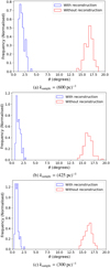 |
Fig. 4 Histograms of the deviation angle between the true arrival direction of UHECRs and the one obtained by backtracking through the magnetic field, as reconstructed using local data sampled at three different mean rates ksample = (600 pc)−1, (425 pc)−1, and (300 pc)−1 (blue). For each mean sampling rate, we considered 100 independent GMFs. The observed arrival direction, the charge, and lab-frame energy were assumed to be known and are (0,0,− 1)T, +e, and 5 × 10¹⁹ eV, respectively. The turbulent-to-uniform magnitude ratio (Eq. (10)) was set at λ = 0.2. For reference, we also plot the same angle by completely neglecting the effect of the GMF on the particle’s trajectory (red). It can be seen that local and homogeneously distributed GMF data significantly improve our estimate of the true arrival directions of UHECRs, and that there is successive improvement as ksample becomes larger, as expected. |
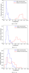 |
Fig. 5 Histograms of the deviation angle between the true arrival direction of UHECRs and the one obtained by backtracking through the magnetic field, as reconstructed using local data sampled at three turbulent-to-uniform ratios λ = 0.5, λ = 1, and λ = ∞, for λ defined in Eq. (10). For a value of λ, we considered 100 independent GMFs. The observed arrival direction, the charge, and lab-frame energy were assumed to be known and are (0, 0, −1)T, +e, and 5 × 10¹⁹ eV, respectively. The sampling rate (Eq. (15)) was set at ksample = 600 pc. For reference, we also plot the same angle by completely neglecting the effect of the GMF on the particle’s trajectory (red). It can be seen that as λ becomes larger, the deviations in the original direction as obtained by backtracking through the reconstructed GMF and the true arrival direction become more dispersed, while the observed discrepancy diffuses toward smaller angles. |
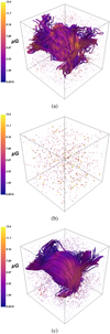 |
Fig. 6 Reconstruction of an isotropically turbulent 3D magnetic field within a cube of side L = 3 kpc. Top: the ground truth; an isotropically turbulent GMF with an RMS magnitude of 5 µG. The colormap denotes the vector’s magnitude. Middle: local data sampled uniformly. The mean distance between each data point is 300 pc. The colormap is saturated at the maximum magnitude that appears in Fig. 6a. Bottom: the mean of the approximating Gaussian posterior distribution attained via the geoVI algorithmn based on the data provided in Fig. 6b. |
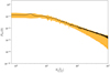 |
Fig. 7 As with Fig. 2, but for the case displayed in Fig. 6. In this case, all modes are relevant and well constrained, as opposed to the case of Fig. 2. Furthermore, we note that as k becomes larger the posterior of the power spectrum starts deviating from that of the signal, implying a loss of information at smaller lengthscales, as observed in Fig. 6. |
4 Summary, conclusions, and outlook
4.1 Summary
In this work, we used 3D local and sparse mock observations of the GMF scattered across a cubic domain of 3 kpc sides within the Galaxy, which are statistically uniformly distributed, in order to obtain the posterior distribution of the UHECR arrival directions before they entered the domain of influence of the GMF. We considered a two-component field, which was comprised of a uniform and random (turbulent) part, for various relative strengths between the two components. We used techniques from information field theory and geoVI in order to construct a systematic way of calculating sample configurations from the posterior PDF. We adapted the correlated field model of IFT to include the case divergence-free vector field such as the GMF, so that the divergence-free condition was also taken into account during the computation of the posterior samples.
Once the above framework was established, we used it to test the quality of our reconstruction by comparing it to the ground truth, for various cases of sampling rates and turbulent-to-uniform ratios. By backtracking a UHECR of known arrival direction and a rigidity (energy per unit charge) equal to 5 × 10¹⁹ V through sample configurations drawn from the posterior PDF for the GMF given the sparse and local mock data, we calculated their reconstructed direction, thus producing a posterior distribution for the true arrival directions. For an ensemble of GMFs sharing the same turbulence-to-uniform ratios and the same mean sampling rate, we were able to estimate the PDF of the mean angle between the true arrival direction and the ones obtained by backtracking through posterior samples, θ, and we were able to show that, in the case of weak turbulence, very modest sampling rates are needed in order for the predictions to not deviate from the true arrival direction by more than a few degrees in relative angle. In particular, for a mean distance of 600 pc between each measurement, the vast majority of the relative angles between the inferred arrival directions and the true ones are below ~3°, for the cases considered. For increasing sampling rates, our results become increasingly better, as should be expected. For reference, completely neglecting the information provided by the local and sparse data, and thus also neglecting the effect of the GMF, results in a relative angle between the observed arrival direction and the true one (θ0) with a mean value, θ0 ~ 15°.
As soon as the turbulent component starts dominating over the uniform one, our results deteriorate, and in the extreme case of fully isotropic turbulence there is a significant overlap between the PDF for θ and θ0. However, even in this extreme and unrealistic case, the local and sparse GMF data still provide a significant improvement in determining the true arrival directions, and by extension the location UHECR sources.
4.2 Conclusions
In conclusion, our results are briefly summarized as follows:
We have developed a systematic framework, based on information field theory, that infers the posterior distribution of the true arrival directions of UHECRs, given sparse and local data for the GMF scattered within a region of the Galaxy.
For weakly turbulent fields, and by using uniformly sampled local data of the GMF with an average S/N of two, we are able to correct for the effect of the GMF to within θ ~ 3°, where θ is the angle between the inferred arrival direction and the true arrival direction. The required mean distance between each measurement can be as large as 600 pc in this case. In applications to real data, the locations of the data points will coincide with the locations of molecular clouds, and a mean distance of ~600 pc is a rather conservative estimate.
In the extreme but unrealistic case of an isotropically turbulent GMF, our results are worse compared to the case of a dominating structured field, but local data can still substantially improve our knowledge on the true arrival directions of UHECRs, and hence on the identity of their sources.
Other simple inference methods, specifically a vector mean of the data points or a nearest-neighbor estimate of the GMF, require very weak turbulence and/or high sampling rates, and even in this case they do not quantify the uncertainty of the inference in a statistically rigorous way. These shortcomings are addressed by the IFT-based method introduced in this work, as it produces samples of the posterior distribution of arrival directions instead of a single estimate, and no prior assumption about the relative strength of the turbulent component or the sampling rate is required.
4.3 Final comments and outlook
In this work, the data points were chosen to have a constant mean sampling rate throughout the domain of study, with the mean distance between the measurements serving as an adjustable parameter. However, in real applications this parameter is not set by us, but rather by Nature, as our measurements will be localized wherever HI clouds exist inside the domain within which we wish to reconstruct the GMF. In particular, their spacing will depend on the distance from the Galactic plane. It might be the case that the assumption of statistical homogeneity of data introduces biases into our results. In future work, we will consider the case of inferring UHECRs’ true arrival directions by using data from MHD simulations of Galactic evolution in Milky Way-like galaxies, where our mock observations will not be chosen at random by a predetermined distribution, but rather from the distribution of clouds as given by the simulation data. It should also be noted that 3D information on each synthetic data point is a rather idealized situation; real data will mainly consist of PoS information alone, often even integrated (with some structured weighting) along the LoS. However, in the small deflection case that is relevant for our problem, the PoS component is expected to dominate the UHECR path’s deflection, since the observed velocity is parallel to the LoS. This issue will be addressed in detail in future work. Finally, we like to add that for any UHECR source that could be identified, the difference between the observed and initial travel directions of the corresponding UHECRs will then provide information on the intergalactic magnetic field.
Acknowledgements
A.T. and V.P. acknowledge support from the Foundation of Research and Technology – Hellas Synergy Grants Program through project MagMASim, jointly implemented by the Institute of Astrophysics and the Institute of Applied and Computational Mathematics. A.T. acknowledges support by the Hellenic Foundation for Research and Innovation (H.F.R.I.) under the “Third Call for H.F.R.I. Scholarships for PhD Candidates” (Project 5332). V.P. acknowledges support by the Hellenic Foundation for Research and Innovation (H.F.R.I.) under the “First Call for H.F.R.I. Research Projects to support Faculty members and Researchers and the procurement of high-cost research equipment grant” (Project 1552 CIRCE). A.T. would like to thank Vincent Pelgrims, Raphael Skalidis, Georgia V. Panopoulou, and Konstantinos Tassis for helpful tips and stimulating discussions. G.E. acknowledges the support of the German Academic Scholarship Foundation in the form of a PhD scholarship (“Promotionsstipendium der Studienstiftung des Deutschen Volkes”).
Appendix A Geometric variational inference (geoVI)
In this appendix we provide a brief step-by-step overview of the geoVI algorithm, which is the main algorithm used to approximate the posterior distribution of the magnetic field, given sparse and local data. The idea is to approximate the true posterior, P, with an approximate one, Q. The approximate posterior, Q, is chosen such that the Kullback-Leibler divergence (Kullback & Leibler 1951),
 (A.1)
(A.1)
between the actual posterior, P, and an approximate posterior, Q, is minimized. The main idea of geoVI is to achieve this minimization in a new coordinate system, chosen such that P - in the new coordinate system - locally closely resembles a normalized standard distribution. Once this is done, the approximating posterior, Q, is chosen to be of the form (3). Then, the mean and covariance are chosen as the parameters with respect to which the KL divergence is minimized.
- 1.
First, a coordinate transformation, φ = f (ξ), is performed, such that the new prior is Gaussian with unit covariance and zero mean, the standardized coordinate system. Henceforth, the measure 𝔇ξ signifies integration over all possible configurations of the vector field, ξ.
- 2.
In this new coordinate system, we calculate the Fisher information metric (Amari 2016), ℳ(ξ), for the likelihood, marginalising the data and joining it with the unit prior metric, ⊮. Intuitively, this may be regarded as a metric over the statistical manifold associated with the likelihood P(d|ξ).
- 3.
We seek another transformation, 𝑔, on top of the original f, that turns ℳ + ⊮ into the Euclidean metric, locally. The motivation is that in this coordinate system, since the geometry of the statistical manifold is as simple as possible, the original posterior is more likely to be accurately described by a Gaussian. The accuracy of the step depends on the choice of the expansion point for the local transformation. It can be computed locally around the mean of the approximating Gaussian in this new coordinate system.
- 4.
The KL-divergence (A.1) is minimized in the coordinate system to which g maps with respect to the mean referred to in the previous step, using a second-order quasi-Newton method called the Newton conjugate gradient (NewtonCG) (Nocedal & Wright 2006). This is achieved by drawing sample configurations and using them to compute the KL divergence, minimising it with respect to the mean.
Appendix B Back-propagating the UHECRs through the GMF
The equations of motion for a relativistic charged particle of charge, q, in a static magnetic field in the lab frame, B = B(x), are
 (B.1)
(B.1)
and
 (B.2)
(B.2)
where γ is the particle’s Lorentz factor, and v its velocity. Equation (B.2) follows from the absence of an electric field. Substituting equation (B.2) into (B.3), we get
 (B.3)
(B.3)
where E is the particle’s lab-frame energy.
If δt is a small time interval, then the change in the velocity during the interval, δt, is
 (B.4)
(B.4)
Using equation (B.3), we may write
 (B.5)
(B.5)
where we divided both sides by |v| ≃ c, and  is the velocity’s direction at any given time. Substituting equation (B.4) into (B.5) and solving for v(t − δt), we obtain
 (B.6)
(B.6)
where q = Ze, with e being the electron charge and Z the atomic number of the UHECR.
If we are also given the position of the UHECR at time t, and we wish to calculate it at time t - t, then we may write
 (B.7)
(B.7)
where we once again made the assumption |v| ≃ c throughout the particle’s path.
Therefore, if we are given the position, charge, lab-frame energy, and observed arrival direction of a UHECR, we can use equations (B.6) and (B.7) iteratively in order to solve the equations of motion numerically. We choose δt in the iterative process such that the length, côt, is equal to the resolution; the total domain is subdivided into voxels of side length cδt, within which the GMF is assumed to be constant. For this work, this amounts to setting cδt = 60 pc, while the side of the total cubic domain is 3 kpc.
Finally, once the initial arrival direction is obtained - this happens when the coordinates of the UHECR’s location exceed the boundaries of the domain - it is translated into galactic coordinates via the equations
 (B.8)
(B.8)
where if ℓ < 0, 2π is added to avoid negative angles.
References
- Abbasi, R. U., Abe, M., Abu-Zayyad, T., et al. 2014, ApJ, 790, L21 [NASA ADS] [CrossRef] [Google Scholar]
- Amari, S.-i. 2016, Invariant Geometry of Manifold of Probability Distributions (Tokyo: Springer Japan) [Google Scholar]
- Andersson, B. G., Lazarian, A., & Vaillancourt, J. E. 2015, ARA&A, 53, 501 [Google Scholar]
- Arras, P., Baltac, M., Ensslin, T. A., et al. 2019, Astrophysics Source Code Library [record ascl:1903.008] [Google Scholar]
- Arras, P., Frank, P., Haim, P., et al. 2022, Nat. Astron., 6, 259 [NASA ADS] [CrossRef] [Google Scholar]
- Bailer-Jones, C. A. L., Rybizki, J., Fouesneau, M., Demleitner, M., & Andrae, R. 2021, AJ, 161, 147 [Google Scholar]
- Bhattacharjee, P., & Sigl, G. 2000, Phys. Rep., 327, 109 [NASA ADS] [CrossRef] [Google Scholar]
- Chandrasekhar, S., & Fermi, E. 1953, ApJ, 118, 113 [Google Scholar]
- Davis, L. 1951, Phys. Rev., 81, 890 [Google Scholar]
- di Matteo, A., Anchordoqui, L., Bister, T., et al. 2023, EPJ Web Conf., 283, 03002 [CrossRef] [EDP Sciences] [Google Scholar]
- Enßlin, T. 2022, Entropy, 24, 374 [CrossRef] [Google Scholar]
- Enßlin, T. A., Frommert, M., & Kitaura, F. S. 2009, Phys. Rev. D, 80, 105005 [Google Scholar]
- Frank, P., Leike, R., & Enßlin, T. A. 2021, Entropy, 23, 853 [NASA ADS] [CrossRef] [Google Scholar]
- Gaia Collaboration (Prusti, T., et al.) 2016, A&A, 595, A1 [NASA ADS] [CrossRef] [EDP Sciences] [Google Scholar]
- Gaia Collaboration (Brown, A. G. A., et al.) 2021, A&A, 649, A1 [NASA ADS] [CrossRef] [EDP Sciences] [Google Scholar]
- Green, G. M., Schlafly, E., Zucker, C., Speagle, J. S., & Finkbeiner, D. 2019, ApJ, 887, 93 [NASA ADS] [CrossRef] [Google Scholar]
- Guardiani, M., Frank, P., Kostic, A., et al. 2022, PLoS ONE, 17, e0275011 [NASA ADS] [CrossRef] [Google Scholar]
- Jaffe, T., Waelkens, A., Reinecke, M., Kitaura, F. S., & Ensslin, T. A. 2012, Astrophysics Source Code Library [record ascl:1201.014] [Google Scholar]
- Jansson, R., & Farrar, G. R. 2012a, ApJ, 757, 14 [NASA ADS] [CrossRef] [Google Scholar]
- Jansson, R., & Farrar, G. R. 2012b, ApJ, 761, L11 [NASA ADS] [CrossRef] [Google Scholar]
- Kawata, K., di Matteo, A., Fujii, T., et al. 2019, in International Cosmic Ray Conference, 36, 36th International Cosmic Ray Conference (ICRC2019), 310 [NASA ADS] [Google Scholar]
- Kullback, S., & Leibler, R. A. 1951, Ann. Math. Statist., 22, 79 [Google Scholar]
- Lallement, R., Babusiaux, C., Vergely, J. L., et al. 2019, A&A, 625, A135 [NASA ADS] [CrossRef] [EDP Sciences] [Google Scholar]
- Leike, R. H., & Enßlin, T. A. 2019, A&A, 631, A32 [NASA ADS] [CrossRef] [EDP Sciences] [Google Scholar]
- Magalhães, A. M. 2012, in Science from the Next Generation Imaging and Spectroscopic Surveys, 7 [Google Scholar]
- Mahalanobis, P. C. 1936, Proc. Natl. Inst. Sci. (India), 2, 6 [Google Scholar]
- Maharana, S., Kypriotakis, J. A., Ramaprakash, A. N., et al. 2021, J. Astron. Telescopes Instrum. Syst., 7, 014004 [NASA ADS] [Google Scholar]
- Maharana, S., Anche, R. M., Ramaprakash, A. N., et al. 2022, J. Astron. Telescopes Instrum. Syst., 8, 038004 [NASA ADS] [Google Scholar]
- Nocedal, Jorge, P., & Wright, S. J. 2006, Large-Scale Unconstrained Optimization (New York, NY: Springer New York), 164 [Google Scholar]
- Panopoulou, G. V., Psaradaki, I., Skalidis, R., Tassis, K., & Andrews, J. J. 2017, MNRAS, 466, 2529 [NASA ADS] [CrossRef] [Google Scholar]
- Pavlidou, V., & Tomaras, T. 2019, Phys. Rev. D, 99, 123016 [CrossRef] [Google Scholar]
- Pelgrims, V., Panopoulou, G. V., Tassis, K., et al. 2023, A&A, 670, A164 [NASA ADS] [CrossRef] [EDP Sciences] [Google Scholar]
- Pierre Auger Collaboration (Aab, A., et al.) 2017, Science, 357, 1266 [NASA ADS] [CrossRef] [Google Scholar]
- Romanopoulos, S., Pavlidou, V., & Tomaras, T. 2022a, arXiv e-prints [arXiv:2206.14837] [Google Scholar]
- Romanopoulos, S., Pavlidou, V., & Tomaras, T. 2022b, in 37th International Cosmic Ray Conference, 12-23 July 2021, Berlin, 475 [Google Scholar]
- Selig, M., Bell, M. R., Junklewitz, H., et al. 2013, A&A, 554, A26 [NASA ADS] [CrossRef] [EDP Sciences] [Google Scholar]
- Skalidis, R., & Tassis, K. 2021, A&A, 647, A186 [NASA ADS] [CrossRef] [EDP Sciences] [Google Scholar]
- Skalidis, R., Sternberg, J., Beattie, J. R., Pavlidou, V., & Tassis, K. 2021, A&A, 656, A118 [NASA ADS] [CrossRef] [EDP Sciences] [Google Scholar]
- Steininger, T., Dixit, J., Frank, P., et al. 2019, Ann. Physik, 531, 1800290 [NASA ADS] [CrossRef] [Google Scholar]
- Sun, X.-H., & Reich, W. 2010, Res. Astron. Astrophys., 10, 1287 [Google Scholar]
- Sun, X. H., Reich, W., Waelkens, A., & Enßlin, T. A. 2008, A&A, 477, 573 [NASA ADS] [CrossRef] [EDP Sciences] [Google Scholar]
- Tahani, M., Glover, J., Lupypciw, W., et al. 2022a, A&A, 660, L7 [NASA ADS] [CrossRef] [EDP Sciences] [Google Scholar]
- Tahani, M., Lupypciw, W., Glover, J., et al. 2022b, A&A, 660, A97 [NASA ADS] [CrossRef] [EDP Sciences] [Google Scholar]
- Takami, H., & Sato, K. 2010, ApJ, 724, 1456 [NASA ADS] [CrossRef] [Google Scholar]
- Tassis, K., Ramaprakash, A. N., Readhead, A. C. S., et al. 2018, arXiv e-prints [arXiv:1810.05652] [Google Scholar]
- Torres, D. F., & Anchordoqui, L. A. 2004, Rep. Progr. Phys., 67, 1663 [CrossRef] [Google Scholar]
Helicity would add a complex, antisymmetric term of the form iɛijiklH(k), with H(k) being the real helicity spectrum, which satisfies −P(k) < H(k) < P(k).
Here, the term ‘energy’ is used in the context of signal processing, and it does not refer to physical energy, although the two are related.
In addition to the reference provided, the reader is advised to look at https://ift.pages.mpcdf.de/public/dense/ for further information.
All Tables
All Figures
|
Fig. 1 Reconstruction of a 3D magnetic field within a cube of side L = 3 = kpc. Top: the ground truth; a uniform field parallel to the x − y plane with magnitude 5 μG, plus a turbulent, random, field with an RMS magnitude of 1 μG, corresponding to λ = 0.2 in Eq. (10). Middle: local data sampled randomly, with a constant mean sampling rate (600 pc)−1. The colormap is saturated at the maximum magnitude that appears in Fig. 1a. Bottom: the mean of the approximating posterior distribution attained via the geoVI algorithmn based on the data provided in Fig. 1b. |
| In the text | |
|
Fig. 2 The three-dimensional power spectrum, P3D(k), corresponding to the example showcased in Fig. 1. The black line is the power spectrum of the mock signal, while the orange envelope encompasses the posterior samples, providing the variance for the posterior mean power spectrum estimate. The wavevector, k, is given in units of 2π/N. The large scatter is due to the fact that we have few and noisy data points, in a signal that is dominated by its uniform component, and thus the modes with k > 0 are poorly constrained. |
| In the text | |
|
Fig. 3 Plane of the sky projections of the UHECR arrival directions as inferred given local and sparse GMF data based on 100 posterior samples (viridis colormap). The GMF reconstruction problem is the one shown in Fig. 1. The red star denotes the true arrival direction, while the black star denotes the observed arrival direction, and they are found 1.6σ and 22.8σ from the posterior’s mean, respectively. For comparison, we also inferred the UHECR arrival direction using a simple vector mean of all the GMF data points (blue star), as well as a a nearest-neighbor estimate (pink star), where at each point the GMF was assumed to be that dictated by the nearest available data point. These simple reconstruction methods do not provide an uncertainty quantification. In addition, they tacitly assume either a low λ, or data points that are populated densely enough – something that cannot be expected from the distribution of dust clouds in real life applications. |
| In the text | |
|
Fig. 4 Histograms of the deviation angle between the true arrival direction of UHECRs and the one obtained by backtracking through the magnetic field, as reconstructed using local data sampled at three different mean rates ksample = (600 pc)−1, (425 pc)−1, and (300 pc)−1 (blue). For each mean sampling rate, we considered 100 independent GMFs. The observed arrival direction, the charge, and lab-frame energy were assumed to be known and are (0,0,− 1)T, +e, and 5 × 10¹⁹ eV, respectively. The turbulent-to-uniform magnitude ratio (Eq. (10)) was set at λ = 0.2. For reference, we also plot the same angle by completely neglecting the effect of the GMF on the particle’s trajectory (red). It can be seen that local and homogeneously distributed GMF data significantly improve our estimate of the true arrival directions of UHECRs, and that there is successive improvement as ksample becomes larger, as expected. |
| In the text | |
|
Fig. 5 Histograms of the deviation angle between the true arrival direction of UHECRs and the one obtained by backtracking through the magnetic field, as reconstructed using local data sampled at three turbulent-to-uniform ratios λ = 0.5, λ = 1, and λ = ∞, for λ defined in Eq. (10). For a value of λ, we considered 100 independent GMFs. The observed arrival direction, the charge, and lab-frame energy were assumed to be known and are (0, 0, −1)T, +e, and 5 × 10¹⁹ eV, respectively. The sampling rate (Eq. (15)) was set at ksample = 600 pc. For reference, we also plot the same angle by completely neglecting the effect of the GMF on the particle’s trajectory (red). It can be seen that as λ becomes larger, the deviations in the original direction as obtained by backtracking through the reconstructed GMF and the true arrival direction become more dispersed, while the observed discrepancy diffuses toward smaller angles. |
| In the text | |
|
Fig. 6 Reconstruction of an isotropically turbulent 3D magnetic field within a cube of side L = 3 kpc. Top: the ground truth; an isotropically turbulent GMF with an RMS magnitude of 5 µG. The colormap denotes the vector’s magnitude. Middle: local data sampled uniformly. The mean distance between each data point is 300 pc. The colormap is saturated at the maximum magnitude that appears in Fig. 6a. Bottom: the mean of the approximating Gaussian posterior distribution attained via the geoVI algorithmn based on the data provided in Fig. 6b. |
| In the text | |
|
Fig. 7 As with Fig. 2, but for the case displayed in Fig. 6. In this case, all modes are relevant and well constrained, as opposed to the case of Fig. 2. Furthermore, we note that as k becomes larger the posterior of the power spectrum starts deviating from that of the signal, implying a loss of information at smaller lengthscales, as observed in Fig. 6. |
| In the text | |
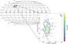 |
Fig. 8 As with Fig. 3, but for the turbulent magnetic field case displayed in Fig. 6. |
| In the text | |
Current usage metrics show cumulative count of Article Views (full-text article views including HTML views, PDF and ePub downloads, according to the available data) and Abstracts Views on Vision4Press platform.
Data correspond to usage on the plateform after 2015. The current usage metrics is available 48-96 hours after online publication and is updated daily on week days.
Initial download of the metrics may take a while.