| Issue |
A&A
Volume 681, January 2024
|
|
|---|---|---|
| Article Number | A24 | |
| Number of page(s) | 13 | |
| Section | Galactic structure, stellar clusters and populations | |
| DOI | https://doi.org/10.1051/0004-6361/202345959 | |
| Published online | 03 January 2024 | |
A robust automated machine-learning method for the identification of star clusters in the central region of the Small Magellanic Cloud
1
Department of Physics, National and Kapodistrian University of Athens, Panepistimiopolis, Zografos 15784, Greece
e-mail: This email address is being protected from spambots. You need JavaScript enabled to view it.
2
University of Crete, Physics Department & Institute of Theoretical & Computational Physics, 71003 Heraklion, Crete, Greece
3
Foundation for Research and Technology-Hellas, 71110 Heraklion, Crete, Greece
4
Department of Physics, Box 41051, Science Building, Texas Tech University, Lubbock, TX 79409-1051, USA
5
Harvard-Smithsonian Center for Astrophysics, 60 Garden Street, Cambridge, MA 02138, USA
Received:
18
January
2023
Accepted:
30
August
2023
Abstract
Aims. We developed a cluster-detection method based on the code DBSCAN to identify star clusters in the central region of the Small Magellanic Cloud (SMC).
Methods. Two approaches were used to determine the values of the free parameters of DBSCAN. They agree well with each other and can be used in the fields that are studied without any a priori knowledge of clustering, characteristic scales, or background density. We validated the success of the DBSCAN cluster-detection method on recent cluster catalogues after introducing a cluster-classification scheme based on three diagnostics that relie on colour-magnitude diagrams and growth curves. We used data from the Magellan Telescope at the Las Campanas Observatory in Chile and from Gaia Data Release 3.
Results. As a byproduct of the validation process, we revisited objects that were classified as clusters in recent compilations. We found that 40% fail all diagnostics and most probably are not clusters. DBSCAN was very successful in recovering actual clusters with high precision and recall.
Key words: Magellanic Clouds / galaxies: star clusters: general / methods: statistical
© The Authors 2023
 Open Access article, published by EDP Sciences, under the terms of the Creative Commons Attribution License (https://creativecommons.org/licenses/by/4.0), which permits unrestricted use, distribution, and reproduction in any medium, provided the original work is properly cited.
This article is published in open access under the Subscribe to Open model. This email address is being protected from spambots. You need JavaScript enabled to view it. to support open access publication.
1. Introduction
At a distance of about 62 kpc (Scowcroft et al. 2016), the Small Magellanic Cloud (SMC) is the nearest low-metallicity star-forming gas-rich dwarf galaxy. It is a member of a small group of galaxies that is believed to be on its first infall towards the Milky Way (Besla et al. 2016; Hammer et al. 2015). The SMC is interacting with the more massive Large Magellanic Cloud (LMC) and with our Galaxy (D’Onghia & Fox 2016; Besla et al. 2012, 2010). Manifestations of these interactions can be found in morphological characteristics (the SMC Wing, Magellanic Bridge, and the high line-of-sight depth; Subramanian & Subramaniam 2012; Jacyszyn-Dobrzeniecka et al. 2017; Muraveva et al. 2018), as well as in the history of star and cluster formation. Bursts of star cluster formation might be linked to close encounters between the two clouds (e.g. Nayak et al. 2018; Bekki 2007).
Star clusters constitute an important component of a galaxy and play a crucial role in our understanding of star formation, stellar evolution, and galactic dynamics. The identification of star clusters in the SMC is an ongoing endeavour. The quest for SMC star clusters started almost a century ago (Shapley & Wilson 1925). It was originally largely based on visual inspection of photographic plates (Hodge & Wright 1974; Bruck 1975) and subsequently of CCD images, starting with the study by Hodge (1986). Machine-learning and data-mining methods and techniques have been employed only recently to detect star clusters in the Magellanic Clouds.
The detection of star clusters is not as straightforward as it might seem, especially when considering relatively low number-density clusters projected on a dense and variable background. This means that the spatial resolution of the data that are used is a crucial factor, particularly when the cluster identification is based only on projected spatial overdensities. Identified star cluster candidates were frequently later discarded as false detections when better-quality (resolution) data became available. Future availability of accurate proper motions (and radial velocities) is expected to improve the reliability of the star cluster identification.
Many authors have applied several different methods and criteria. Machine-learning approaches are the most recent addition. Schmeja (2011) compared four different methods of identifying stellar number-density enhancements in a field. The computation time of each algorithm was different and depended on the size, the properties of the area under investigation, and the purpose of the study. Bitsakis et al. (2018) followed an automated detection method and found a large number of new candidate clusters in the central regions of the SMC, the great majority of which were later disputed or classified as stellar associations (Piatti 2018; Bica et al. 2020).
In addition to differences caused by different detection methods and selection criteria, there are also effects related to the wavelength region used for the identification of clusters. Using near-infrared data, Piatti (2017, 2016) detected new candidate clusters in the central regions of the SMC that are hardly recognizable on optical images without the aid of a robust analysis based on colour-magnitude diagrams (CMDs) corrected for field star contamination. Recently, Bica et al. (2020) combined results from different catalogues and detection methods to compile a list of 2741 clusters, associations, and candidates (in the SMC and the Magellanic Bridge). This list constitutes the reference catalogue for the present study.
The mass and age distribution of the star cluster is a significant component in our understanding of the evolution of a galaxy. The age distribution of SMC star clusters has been the subject of several studies. Chiosi et al. (2006) found an enhancement of cluster formation between 15 and 90 Myr, while Glatt et al. (2010) identified two periods of enhanced star cluster formation at 160 Myr and 630 Myr. The youngest clusters in the SMC seem to reside in supergiant and giant shells of HI, intershell regions, and in regions with a strong Hα emission, suggesting that their formation is related to the expansion of shells and shell-shell interactions (Glatt et al. 2010).
Piatti et al. (2007) found indications that many young clusters are located closer to the centre of the SMC. On the other hand, Piatti (2021) suggested that the more massive star clusters are located in the outer regions. Other recent extensive studies of the age distribution of star clusters in the SMC (Nayak et al. 2018; Narloch et al. 2021) showed that clusters in the northern part of the SMC are generally younger than those in the south, while cluster formation is continuous in the centre. There is also evidence that the peak of the cluster age distribution is the same in both clouds (Nayak et al. 2016), supporting the hypothesis that their interaction affects their evolution significantly.
Although all these studies provide valuable insights into the evolution of the SMC, it is also clear that large numbers of erroneously classified clusters can lead to biased interpretations. In this paper, we revisit the star cluster population in the central regions of the SMC with high spatial resolution data obtained with the Magellan Telescope (Strantzalis et al. 2019) and the recently released Gaia DR3 (Gaia Collaboration 2021). The aim of the paper is first to establish a set of well-defined diagnostics that an object must satisfy in order to be considered a star cluster. Based on these diagnostics, we then reclassify 90 star clusters from the Bica et al. (2020) catalogue that are located in the central regions of the SMC covered by the Inamori Magellan Areal Spectrograph (IMACS) data. Using the confirmed set of star clusters as reference, we develop and validate an automated method for the identification of star clusters in the central regions of the SMC based on the density-based spatial clustering of applications with noise (DBSCAN) algorithm and Gaia DR3 data. Section 2 presents the observational data, followed by Sect. 3, in which we introduce our established diagnostics and discuss the outcomes when applied to catalogued star clusters. In Sect. 4 we demonstrate the implementation of DBSCAN for the identification of star clusters and validate the results. Lastly, in Sect. 5, we summarize our conclusions.
2. Data
Two sets of data were used in this paper. The first set consists of photometric data in the Johnson B and I filters obtained with the 6.5 m Magellan Telescope at the Las Campanas Observatory in Chile. The data cover a total area of 0.5 deg2 in the central region of the SMC and comprise four IMACS fields of 0.14 deg2 each. A total of 1 068 903 sources were detected with magnitude errors smaller than 0.2mag. The data analysis leading to the derivation of B and I magnitudes (down to a magnitude limit of B ≃ 24), as well as the error budget and completeness estimates, are fully described in Strantzalis et al. (2019). The high spatial resolution and depth of these data render them valuable for the characterisation of star clusters. However, inhomogeneities are caused by the gaps between the different CCDs in the IMACS camera, which can cause problems in the automated identification of star clusters (Sect. 4). To rectify this, we used Gaia DR3 data covering the same regions on the sky. These data, which constitute our second data set, are shallower (with a limiting magnitude ≃20.5 mag), but they are very useful because they are homogeneous and show no gaps and are thus well suited for DBSCAN. However, they are known to be significantly incomplete in regions of high source density, especially for magnitudes fainter than G = 21 mag (Cantat-Gaudin et al. 2023; Castro-Ginard et al. 2023). They also provide information for brighter stars that are saturated in the IMACS data and are used to construct the cluster growth curves. To avoid contamination from galactic stars, we applied an upper parallax limit of 0.2 mas. The relatively bright limiting magnitude of the Gaia data implies that in the case of old clusters, only the red clump and giants would be visible on the CMD, thus rendering their detection more difficult.
3. Validation of the star clusters
3.1. Validation diagnostics
As previously mentioned, the identification of star clusters is affected by the spatial resolution of the data, their photometric depth, the wavelength region, and the method. Our goal was to employ a suite of different diagnostics to verify in a homogeneous and robust manner the cluster classification of the objects in the reference catalogue of Bica et al. (2020), which lie in the IMACS fields. This catalogue is a comprehensive compilation of star clusters, associations, and related extended objects in the SMC and the Magellanic Bridge. It has 2741 entries, which is twice as many as a previous version of the catalogue from more than a decade ago (Bica et al. 2008). The main observational properties used by Bica et al. (2020) to classify objects as clusters include central concentration and density contrast against the surrounding field, often using multi-colour information (see also Bica et al. 2019).
The Bica et al. (2020) catalogue contains 90 objects with classifications C (cluster), CA (cluster association), and CN (cluster nebula) that lie in our fields. We did not consider systems classified as associations (A, AC, and AN) because they are generally very extended, loose, and likely unbound structures. We also excluded 19 systems that were discovered using the Vista Magellanic Cloud near-infrared survey (Piatti et al. 2016) because they are generally not identifiable in optical images. Figure 1 shows the spatial distribution of the C, CA and CN (shown with red, magenta, and green symbols, respectively) objects on a 24 μm map of the SMC; the four IMACS fields we used in our analysis are indicated with white circles. None of the 45 newly discovered faint clusters (yellow circles) and candidates in Bica et al. (2020) are located in our fields.
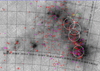 |
Fig. 1. Spatial distribution of the star clusters of types C, CA, and CN (shown with red, magenta, and green circles, respectively, and the sizes are proportional to the cluster radii) from the catalogue of Bica et al. (2020) overlaid on an image of the SMC obtained with Spitzer-MIPS at 24 μm. The yellow circles represent the new candidate clusters, and the IMACS fields are indicated with white circles. The symbol sizes are proportional to the cluster radii. |
For these 90 objects, we constructed CMDs and growth curves. On the basis of these, we developed three cluster diagnostics that are described in detail in the following paragraphs, to assign a quality class to the systems we studied: Class 3 for clusters that are considered as certain, Class 2 for probable clusters, Class 1 for systems that are probably not clusters, and Class 0 for systems that are not confirmed as clusters. Class 3 clusters satisfy all three diagnostics, Class 2 clusters satisfy two diagnostics, Class 1 clusters satisfy one diagnostic, and Class 0 clusters satisfy no diagnostic.
The first diagnostic, based on Gaia DR3 data, involves the examination of the growth curve of a cluster. This curve shows how the total number of stars within a circular aperture increases in the area around the central coordinates of the cluster as the aperture radius expands. We can quantify this diagnostic by comparing the curve of growth for the stars lying around the centre of the candidate cluster with a curve of growth derived for a uniform spatial distribution of the same (total) number of stars. We evaluated the significance of the difference between the two curves using a Kolmogorov-Smirnov (KS) two-sample test. In order to assess statistical fluctuations, we repeated this analysis 10 000 times using different randomly drawn samples of background distributions. We calculated the mean p-value resulting from the application of the KS test in each iteration. This is important because many clusters have very few (fewer than 50) visible members. For p-values lower than 0.05, the null hypothesis that the two samples come from the same population was rejected. In Fig. 2 (left panels) we show the B-band IMACS images of three objects that satisfy the first diagnostic (B59, B79, and L41), with mean p-values within the range 0.002–1 × 10⁻⁶. The corresponding growth curves are shown in the right panels. These objects also satisfy all other diagnostics (see below), and were hence assigned Class 3. In contrast, in the left panels of Fig. 3, we show examples of objects (BS259, MA222, and H86-123) that do not constitute statistically significant overdensities. In these cases, the p-values lie in the range 0.50–0.61, and hence the growth curves (shown in the right panels) are compatible with those of a uniform distribution. These are examples of Class 0 objects: They fail to satisfy the other diagnostics as well.
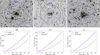 |
Fig. 2. Images and growth curves for objects of Class 3. In all cases, the growth curves for the clusters (shown in blue) differ significantly from the growth curve for a uniform distribution (shown in red). The cluster radius as provided by the reference catalogue is indicated with a blue circle. B-band IMACS images are presented in the top panels and growth curves in the bottom panels for objects B59, B79, and L41. |
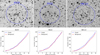 |
Fig. 3. Images and growth curves for the objects of Class 0. In all cases, the growth curves for the clusters (shown in blue) do not differ significantly from the growth curve for an uniform distribution (shown in red). The cluster radius as provided by the reference catalogue is indicated with a blue circle. B-band IMACS images are presented in the top panels and growth curves in the bottom panels for objects BS259, MA222, and H86-123. |
The second and third diagnostics were derived from the cluster CMD, which was constructed using IMACS data. Star clusters have almost simple-population CMDs characteristic of the age and metallicity of the cluster, which are often distinguishable from the surrounding field. The two diagnostics are based on a statistical comparison between the magnitude (for the second diagnostic) and colour (for the third diagnostic) distributions of stars lying along the main sequence (MS) of the candidate cluster and neighbouring field regions (with an equal area), respectively. The MS stars were roughly separated from the red clump and giants using a colour selection, −1.0 ≤ B − I ≤ 0.6. This is sufficient for our purposes. In Fig. 4 we show the CMDs and corresponding magnitude and colour distributions of MS stars for two objects B55 and BS259. On the left, we show the magnitude distribution along the MS for the cluster (blue line) and field (red line) stars. At the top, we show the corresponding colour distributions. The comparison between the blue and red magnitude and colour distributions, that is, between cluster and field, is performed using the KS. The null hypothesis is that the two distributions (cluster and field) are drawn from the same population. As for the first diagnostic, the null hypothesis is rejected for a p-value lower than 0.05. The KS test is performed separately for the magnitude and colour distributions.
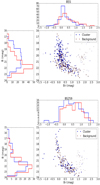 |
Fig. 4. CMDs and magnitude and colour distributions of MS stars for B55 (top) and BS259 (bottom). The blue symbols and lines correspond to the cluster region, and the red symbols and lines to the neighbouring background region of equal area. On the CMD, stars selected to be on the MS are denoted with larger symbols. |
3.2. Results from the cluster validation
All 90 objects from the catalogue of Bica et al. (2020) that are located in our fields were examined using the three diagnostics described in the previous paragraph and were assigned a quality class, as shown in Table 1. Column 1 gives the name of the cluster, Col. 2 the IMACS field in which the cluster is located, Cols. 3 and 4 the J2000 coordinates of the cluster centre as provided by Bica et al. (2020), Col. 5 the cluster type in Bica et al. (2020), Cols. 6–8 the p-values of the three diagnostic tests, and Col. 9 the quality class assigned to each cluster. For Class 3, all three p-values are < 0.05, for Class 2, any two of the three p-values are < 0.05, for Class 1, only one p-value is < 0.05, and for Class 0, all p-values are > 0.05. Inspection of the p-values provided in Table 1 shows that for objects of Classes 2 and 3, the hypothesis that the cluster and field come from the same population is rejected at a very high confidence level. The few exceptions are objects with very few stars on the MS. Out of the 90 objects, 36 (40% of the total) are of Class 0, 24 of Class 1, 11 of Class 2, and only 19 are of Class 3 (21% of the total).
Star clusters in the catalogue of Bica et al. (2020) within the four IMACS fields.
Of the type C systems in Table 1, 39% belong to quality Classes 2 and 3, that is, they are probable or certain star clusters according to our diagnostics. The percentage is similar for CN types (38%) and drops to 15% for CA types. This is expected because CN is suggestive of the presence of nebulosity, and CA alludes to a stellar association appearance. A significant result of this analysis is that more than one-third (35%) of the type C clusters we examined are rejected as bona fide star clusters. These results are summarized in Table 2, which provides the number of Bica et al. (2020) clusters (within the IMACS fields) of types C, CN, and CA that were classified as objects of Class 0, 1, or 2 and 3.
Number of clusters in the catalogue of Bica et al. (2020) of types C, CN, and CA that were assigned Class 0, 1, or 2 and 3.
We compared the age and size distributions of Class 3 and Class 0 objects, as shown in Fig. 5. The ages and radii were taken from Bica et al. (2020). Small clusters (with radii below 10 pc) clearly dominate among the Class 0 objects. A visual inspection shows that many Class 0 systems consist of a small number of bright stars within a small radius that can be easily mistaken for significant overdensities in images with a lower spatial resolution. The age distributions also show significant differences. The age distribution of Class 0 objects clearly peaks around 100 Myr, which is not the case for Class 3 clusters. A similar peak (∼135 Myr) is also displayed by field stars (Nayak et al. 2018). This supports our conclusion that Class 0 objects are consistent with field populations. Class 3 objects range in age from ∼15 Myr to 1.1 Gyr. We emphasize that Class 0 objects are not older than 3 Gyr. Clusters like this are expected have very few stars on the MS above the limiting magnitude of the IMACS data, which in turn would affect diagnostics 2 and 3.
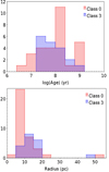 |
Fig. 5. Distribution of ages (top) and radii (bottom) of objects of Class 3 (red line) and Class 0 (blue line). |
Figure 6 clearly shows that field SMC4 contains a larger number of rejected candidate clusters (16), possibly due to the high and variable background and extended regions of significant interstellar absorption (see Strantzalis et al. 2019). The variable background affects the results of star cluster detection algorithms, as we discuss further in the next section. In order to derive a robust identification of star clusters in these environments, we employed an automated classification based on the algorithm DBSCAN, as described in Sect. 4.
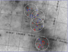 |
Fig. 6. The spatial distribution of the candidate star clusters of Classes 0, (red), 3 (blue) in the SMC (Spitzer). |
4. Approach of the DBSCAN algorithm
4.1. Description of DBSCAN
The DBSCAN is a known machine-learning method (Ester et al. 1996) that has been used by several authors to detect star clusters (Castro-Ginard et al. 2018, 2019, 2020; Hunt & Reffert 2021). In brief, cluster detection is achieved by calculating the density at the location of each point (each star, in our case) and comparing it with the background density. When the difference is sufficient, then the point (star) is considered to belong to an area of local density enhancement.
DBSCAN clustering depends on two parameters: epsilon (eps), and minimum points (MinPts). Eps is a distance threshold that determines the radius around a data point within which other points are considered as neighbours. It sets the maximum distance between two points for them to be considered as part of the same neighbourhood.
MinPts is a numeric parameter that represents the minimum number of points required to form a dense region. It sets the minimum density threshold for a cluster. We note that eps is not directly related to MinPts, but works together with it to define the density of a cluster.
There are four types of points in DBSCAN: core points, directly reachable points, reachable points, and noise points. Core points contain at least MinPts points within an eps distance, including themselves. Core points are considered as central points of a cluster, as they have enough neighbouring points within the specified eps distance to satisfy the density requirement defined by MinPts. Directly reachable points are defined as follows: A point X is directly reachable from point Y if it lies within an eps distance from Y. Directly reachable points do not necessarily satisfy the MinPts condition. A point X is reachable from Y if there is a path X, X1, X2, ..., Y, where each Xi is directly reachable from Xi + 1. All other points are noise points, or outliers. Points X and Y are said to be density connected if there is an intermediate point Z from which both X and Y are reachable.
A cluster in DBSCAN is defined as an over-density of points that are mutually density connected, that is, if a point is reachable from any point of the cluster, then it is a member of the cluster. More specifically, DBSCAN first finds the points in the eps neighbourhood of each point and identifies the core points with more than MinPts neighbours. Subsequently, the algorithm detects the points reachable from the core points found in the previous step. Finally, each point that is not a core point is either assigned to a cluster if it lies within an eps distance from any point of the cluster, otherwise, it is considered as an outlier or noise point. DBSCAN visits each point of the dataset once, the complexity in the worst case scenario being O(n2), where n is the number of points that belong to the dataset.
DBSCAN has the advantage of being able to detect clusters of arbitrary shape. It does not require a prior definition of the number of clusters to be found either, as is the case with other clustering algorithms.
4.2. DBSCAN parameters for the SMC fields
The DBSCAN algorithm was applied to Gaia DR3 data covering the four IMACS fields. The input parameters should be chosen according to the problem domain. As already mentioned, DBSCAN clustering depends on two parameters: MinPts, and eps distance. An automation of star cluster detection using DBSCAN requires an optimization of the values adopted for these parameters for the specific dataset, using either computational or astrophysical considerations.
We explained in the previous section how the two parameters affect the detection, number, and size of clusters. We performed several runs, fixing the MinPts value from 10 to 60 and then determining the eps value, as we show in the next paragraphs. The results were behaviourally similar. For the remaining paper, we therefore adopted a value of 25 for MinPts for the Gaia dataset for completeness reasons.
In order to determine the optimal value for the eps parameter, we performed a k-nearest neighbour (kNN) analysis on the datasets for each IMACS field. In this analysis, we constructed plots of the value of the kNN distance as a function of k that equals the value of MinPts. The kNN distance plot is instrumental to our approach, hence a detailed explanation of what it represents is provided here. The kNN distance is defined as the distance from a point to its k-nearest neighbour. The kNN distance plot displays the kNN distance of all points sorted from the smallest to the largest. For all the points of the dataset, a matrix with k columns, containing the distances to all first, second, and so on to the Nth-nearest neighbours, is returned and plotted. An example of such a plot for field SMC5 is shown in Fig. 7. In this kNN plot, the y-axis represents the average distance of every star in the field from its k-nearest stars, while the x-axis represents the number of stars that lie within this average distance: these curves show an initial rise, a plateau, and then another sharp rise for higher values of k.
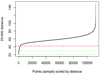 |
Fig. 7. kNN distance plot for field SMC5 (k = MinPts = 25). The two red lines denote the start of the knee formation. The blue line denotes the start of the curve, and the two green lines are placed in the middle between the starting line and the knee formation. The distances are plotted in pixels. |
The kNN plot for the star field data represents the change in star density per average distance: we expect few stars to belong to high-density areas (the first part of the plot before the first knee) and a progressive rise in the number of stars with a lower density up to the point when the density of the background is reached. The first knee indicates the boundary of the over-densities, and the plateau indicates the background density because the stars in the background are uniformly distributed on averaged. There might be none, one, or more than one knee in general, depending on the clumpiness of the source distribution. In the case of the SMC fields we considered, the distance distribution using the kNN method showed very well defined knees that allowed selecting an optimal eps. Based on these plots, we adopted the middle of the rising part of the kNN curve, before the first knee, as the best-fit eps value. This method represents the standard approach for adopting the optimal eps value. However, we developed an additional method that we present in Sect. 4.3. Other methods have been adopted in recent studies to determine the optimal eps value for DBSCAN, which were used to detect open clusters in the Milky Way with Gaia DR2 data. In all cases, the adopted values ranged between zero and the start of the stellar background as identified on the kNN plot. For example, Castro-Ginard et al. (2018) generated a random sample to obtain e(rand) and then adopted the average of e(min) and e(rand) as the eps value. Hunt & Reffert (2021) determined the DBSCAN parameters from the highest curvature point on the nearest-neighbour curve. He et al. (2023) determined the DBSCAN optimal parameters by fitting the kNN curve with the sum of two Gaussian distribution functions.
Table 3 summarizes the results of the kNN analysis for the four SMC fields studied. Column 1 gives the field name, and Col. 2 shows the range of eps values in which the knee forms. In Col. 3 we show a small range of eps distances that reside in the middle of the region prior to the first knee, and finally, the adopted value of the eps parameter for the specified field is provided in Col. 4. It is interesting to note that this value is very similar for all four fields we analysed. This indicates that the areas we examined had similar densities for the cluster and background (field) regions.
Optimal ranges and selected values of eps for each field.
The DBSCAN results were validated using the clusters we studied and classified in Sect. 3. A DBSCAN cluster that coincides with a Class 3 cluster is considered to be a true positive (TP), while a Class 0 object that was not assigned a cluster status by DBSCAN is a true negative (TN). False positives (FP) are objects that are assigned cluster status without actually being clusters, and false negatives (FN) are objects that are not found to be clusters by DBSCAN, but actually are. We used three standard validation metrics, namely, precision, P, defined as P = TP/(TP + FP), recall, R, defined as R = TP/(TP + FN), and F − 1 score, F − 1, which is defined as the harmonic mean of P and R, namely F − 1 = 2PR/(P + R) (see Table 4).
Definitions of TP, FP, TN, and FN.
There is no linear relation between discovery probability and Class number. Cluster Classes 1 and 2 are not found within the eps distance we consider as the best fit. This happens because the optimal eps results in very few or no FP. As the eps value is increased, Classes 1 and 2 appear. With increasing eps, FPs begin to be detected, and only then are Classes 1 and 2 represented.
As a means of validating the choice of the eps value that was achieved following the procedure described above, we ran DBSCAN for a range of eps values from 20 to 40 and calculated P, R, and F − 1 for each experiment. Figure 8 shows the dependence of the P, R, and F − 1 score on the eps value for the four SMC fields we studied. In all cases except for SMC4, the kNN eps values lie within the range of or partially overlap the eps range for which maximum P, R, and F − 1 score values are observed. This is a strong indication that the method we used to determine the optimal eps value is valid. In the case of SMC4, the strong variation in the background across the field renders the adoption of a global eps value somewhat less successful.
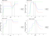 |
Fig. 8. Dependence of precision, recall, and F1-score on the adopted eps value (red, green, and blue lines, respectively) for each one of the four SMC fields. The vertical dotted lines represent the range in the eps values we used, as denoted on Table 3. |
We required from DBSCAN the centres of discovered clusters, and therefore, this gives us the positions of candidate clusters. We are therefore able to cross match the DBSCAN clusters with clusters in the literature becausee we know the Ra/Dec and x/y positions from both cases.
4.3. Core distance-density plots
In the context of DBSCAN, core points are the points for which at least MinPts points are located within an eps distance. It is instructive to see how the core distance (average distance between the core-point stars) correlates with the cluster validation Classes (see Sect. 3.2). For this experiment, we extended our analysis to eps values higher than the optimal values considered in the previous subsection. This allowed us to better differentiate between the behaviour of different cluster Classes because at least some FP will be observed. At the optimal value of eps, FP are very close to zero, as shown by the high precision we presented in the previous subsection. Any eps value higher than the optimal is appropriate for this test. We used the value of 37, but similar results are obtained for higher values. Figure 9 shows three density plots (a density plot is the continuous and smoothed version of the histogram estimated from the data, calculated through a kernel density estimation) of the average distance of the core points for star clusters of Classes 0, 1, 2, and 3. Each line combines the density plots of the average distance of core points per Class. The density plots for Classes 0, 1, and 2 exhibit a distinct peak at high values of core distance, while for Class 3, there is only one peak at low values of core distance. Therefore, these density plots can be used to distinguish high-confidence clusters (Class 3) in a straightforward way. This approach only needs one run of the algorithm. Thus, the reliability of a detected cluster can be extracted from the shape of the core distance-density plot.
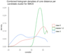 |
Fig. 9. Core distance-density plot combined for Classes 0, 1, and 2 together and 3 for SMC5 and eps 37. |
Further insights into the usefulness of the core distance-density plots can be gained by combining the density plots of all clusters regardless of Class. We constructed the combined core distance-density plots for different eps values. In the left panels of Fig. 10, we show the combined core distance-density plots for three eps values, one high (37), one intermediate (34), and a lower one (31), for field SMC5 as an example. In the right panels of the same figure, we show the corresponding maps of the clusters identified by DBSCAN in each case. The clusters are indicated in red, with the size of the marker corresponding to the actual size of the DBSCAN cluster. Overlaid are encircled numbers providing the cluster Class, when available. For the higher eps values the combined density plots exhibit two distinct peaks. As the eps value is reduced gradually, the height of the second peak (on the right) becomes lower and ultimately vanishes, leaving only the first (left) peak. We find Class 3 clusters when only one peak is visible in the density plot. The density plot requires only very few runs, iterating the algorithm from high to lower eps values.
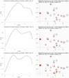 |
Fig. 10. Combined core distance-density plots for all candidate clusters detected by DBSCAN for different eps values (31, 34, and 37) (left) and the positions and shapes of the detected DBSCAN clusters, shown in red, for the corresponding eps values (right). X and Y are pixel positions in the IMACS dataset for field SMC5 (used here as an example). The numbers 0, 1, 2, and 3 shown in circles denote the Class of the actual cluster (if there is one) as determined with the diagnostics of Sect. 3. The extended cluster near the left edge of the maps corresponds to two nearby clusters as detected from DBSCAN with MinPts = 25. This explains the discrepancy when we meticulously count the red clusters and compare them with the cluster count in the title of the plot. |
By using the described technique, we can estimate the appropriate value of eps directly from the core density plot without having a priori knowledge of the class of the objects: we purposefully selected a high value of eps (37 for SMC5), higher than the optimal one (32), which yielded a double-peaked density plot. Gradual reduction of the eps value ultimately yields a single-peaked density plot that corresponds to high confidence clusters of Class 3, without using the technique based on kNN.
It is noteworthy that for the values of the DBSCAN parameters for which we find all high-confidence clusters (Class 3), we do not detect any objects of Class 0 or 1. Cluster Classes 1 and 2 are not found within the optimal eps distance. The reason is that the optimal eps does not result in many false positives. This is a feature of the algorithm. When eps increases and FPs start to appear, Classes 1 and 2 are represented. For parameter values for which we find all clusters of Class 3 and 2, we also find 31% of Class 1 and only 5% of Class 0 objects. Finally, when we adopt the values of eps for which we find 80% of Class 1, then we find 404 additional objects (448% increase of the published sample in these regions), none of which satisfy our diagnostics for being actual star clusters, however.
We can recapitulate the entire method of this section as follows: First, we applied the kNN approach for different MinPts and eps values (which are related via the kNN distance plot and the knee method). We then adopted a MinPts value near the middle of the range of our trials (10–60) and found the eps value via the knee approach. We validated the success of this approach by using the cluster Classes from Sect. 3. Alternatively, in order to distinguish between false and true positives, we can use the core distance-density plot shape for each candidate cluster using a deliberately high eps value and run the algorithm only once. We then applied an additional method for the estimation of eps by using the density histograms of the core distances for all clusters simultaneously (the two-peaks method). The two methods (kNN and density plots) agree well, and both can be used without any a priori knowledge of clustering, characteristic scales, or background density in the fields we studied.
5. Summary and conclusions
The identification of star clusters in the SMC is an ongoing endeavour. It is only relatively recently that machine-learning and data-mining methods and techniques have been employed to detect star clusters in the Magellanic Clouds.
Using high spatial resolution imaging data obtained with the 6.5 m Magellan Telescope (Strantzalis et al. 2019) and Gaia DR3 data, we revisited the SMC star cluster compilation of Bica et al. (2020). Leveraging the high resolution of the Magellan data and the homogeneity of the Gaia data, we reclassified the objects listed in this catalogue that are included in the four fields covered by the study of Strantzalis et al. (2019). The diagnostics used included curve growths and CMDs, as well as statistical indices based on them. Applying these diagnostics, we assigned a Class between 0 and 3 to each object, with 0 indicating a non-cluster, and 3 indicating a high-confidence cluster. According to this classification, 40% of the C, CA and CN clusters in the catalogue of Bica et al. (2020) that lie within the IMACS fields were not confirmed as star clusters. Most of the non-confirmed objects are artefacts caused by the lower spatial resolution of some of the older surveys.
Subsequently, we used the results of this classification to explore and calibrate a star cluster discovery method based on the well-known data clustering algorithm DBSCAN (Ester et al. 1996), which we applied to Gaia DR3 data. DBSCAN is a non-parametric density-based spatial algorithm. Two approaches were used to determine the values of the DBSCAN free parameters (eps and MinPts): kNN, and core distance-density plots. The implementation of both methods is well understood, the choice of values for the variables is justified and reproducible, and both approaches agree regarding the optimal values of the DBSCAN parameters. Finally, none of these approaches requires anything to be known a priori, such as the number of clusters, MinPts, and eps values.
The combined use of the two methods is a very useful tool for the discovery and identification of star clusters in resolved galaxies.
Acknowledgments
The authors thank the anonymous referee for the constructive report which has helped improve the overall quality of the paper. Also, this work presents results from the European Space Agency (ESA) space mission Gaia. Gaia data are being processed by the Gaia Data Processing and Analysis Consortium (DPAC). Funding for the DPAC is provided by national institutions, in particular the institutions participating in the Gaia MultiLateral Agreement (MLA). The Gaia mission website is https://www.cosmos.esa.int/gaia. The Gaia archive website is https://archives.esac.esa.int/gaia. Data available online upon request to the corresponding author.
References
- Bekki, K. 2007, in Triggered Star Formation in a Turbulent ISM, eds. B. G. Elmegreen, & J. Palous, IAU Symp., 237, 373 [Google Scholar]
- Besla, G., Kallivayalil, N., Hernquist, L., et al. 2010, ApJ, 721, L97 [Google Scholar]
- Besla, G., Kallivayalil, N., Hernquist, L., et al. 2012, MNRAS, 421, 2109 [Google Scholar]
- Besla, G., Martínez-Delgado, D., van der Marel, R. P., et al. 2016, ApJ, 825, 20 [Google Scholar]
- Bica, E., Bonatto, C., Dutra, C. M., & Santos, J. F. C. 2008, MNRAS, 389, 678 [Google Scholar]
- Bica, E., Pavani, D. B., Bonatto, C. J., & Lima, E. F. 2019, AJ, 157, 12 [Google Scholar]
- Bica, E., Westera, P., Kerber, L. D. O., et al. 2020, AJ, 159, 82 [Google Scholar]
- Bitsakis, T., González-Lópezlira, R. A., Bonfini, P., et al. 2018, ApJ, 853, 104 [Google Scholar]
- Bruck, M. T. 1975, MNRAS, 173, 327 [NASA ADS] [CrossRef] [Google Scholar]
- Cantat-Gaudin, T., Fouesneau, M., Rix, H.-W., et al. 2023, A&A, 669, A55 [NASA ADS] [CrossRef] [EDP Sciences] [Google Scholar]
- Castro-Ginard, A., Jordi, C., Luri, X., et al. 2018, A&A, 618, A59 [NASA ADS] [CrossRef] [EDP Sciences] [Google Scholar]
- Castro-Ginard, A., Jordi, C., Luri, X., Cantat-Gaudin, T., & Balaguer-Núñez, L. 2019, A&A, 627, A35 [NASA ADS] [CrossRef] [EDP Sciences] [Google Scholar]
- Castro-Ginard, A., Jordi, C., Luri, X., et al. 2020, A&A, 635, A45 [NASA ADS] [CrossRef] [EDP Sciences] [Google Scholar]
- Castro-Ginard, A., Brown, A. G. A., Kostrzewa-Rutkowska, Z., et al. 2023, A&A, 677, A37 [NASA ADS] [CrossRef] [EDP Sciences] [Google Scholar]
- Chiosi, E., Vallenari, A., Held, E. V., Rizzi, L., & Moretti, A. 2006, A&A, 452, 179 [NASA ADS] [CrossRef] [EDP Sciences] [Google Scholar]
- D’Onghia, E., & Fox, A. J. 2016, ARA&A, 54, 363 [CrossRef] [Google Scholar]
- Ester, M., Kriegel, H.-P., Sander, J., Xu, X., et al. 1996, in KDD-96 Proceedings, 96, 226 [NASA ADS] [Google Scholar]
- Gaia Collaboration (Brown, A. G. A., et al.) 2021, A&A, 649, A1 [NASA ADS] [CrossRef] [EDP Sciences] [Google Scholar]
- Glatt, K., Grebel, E. K., & Koch, A. 2010, A&A, 517, A50 [CrossRef] [EDP Sciences] [Google Scholar]
- Hammer, F., Yang, Y. B., Flores, H., Puech, M., & Fouquet, S. 2015, ApJ, 813, 110 [NASA ADS] [CrossRef] [Google Scholar]
- He, Z., Liu, X., Luo, Y., Wang, K., & Jiang, Q. 2023, ApJS, 264, 8 [NASA ADS] [CrossRef] [Google Scholar]
- Hodge, P. 1986, PASP, 98, 1113 [NASA ADS] [CrossRef] [Google Scholar]
- Hodge, P. W., & Wright, F. W. 1974, AJ, 79, 858 [NASA ADS] [CrossRef] [Google Scholar]
- Hunt, E. L., & Reffert, S. 2021, A&A, 646, A104 [NASA ADS] [CrossRef] [EDP Sciences] [Google Scholar]
- Jacyszyn-Dobrzeniecka, A. M., Skowron, D. M., Mróz, P., et al. 2017, Acta Astron., 67, 1 [NASA ADS] [Google Scholar]
- Muraveva, T., Subramanian, S., Clementini, G., et al. 2018, MNRAS, 473, 3131 [Google Scholar]
- Narloch, W., Pietrzyński, G., Gieren, W., et al. 2021, A&A, 647, A135 [NASA ADS] [CrossRef] [EDP Sciences] [Google Scholar]
- Nayak, P. K., Subramaniam, A., Choudhury, S., Indu, G., & Sagar, R. 2016, MNRAS, 463, 1446 [NASA ADS] [CrossRef] [Google Scholar]
- Nayak, P. K., Subramaniam, A., Choudhury, S., & Sagar, R. 2018, A&A, 616, A187 [NASA ADS] [CrossRef] [EDP Sciences] [Google Scholar]
- Piatti, A. E. 2017, ApJ, 834, L14 [Google Scholar]
- Piatti, A. E. 2018, MNRAS, 478, 784 [Google Scholar]
- Piatti, A. E. 2021, A&A, 647, A11 [EDP Sciences] [Google Scholar]
- Piatti, A. E., Sarajedini, A., Geisler, D., Clark, D., & Seguel, J. 2007, MNRAS, 377, 300 [Google Scholar]
- Piatti, A. E., Ivanov, V. D., Rubele, S., et al. 2016, MNRAS, 460, 383 [Google Scholar]
- Schmeja, S. 2011, Astron. Nachr., 332, 172 [NASA ADS] [CrossRef] [Google Scholar]
- Scowcroft, V., Freedman, W. L., Madore, B. F., et al. 2016, ApJ, 816, 49 [NASA ADS] [CrossRef] [Google Scholar]
- Shapley, H., & Wilson, H. H. 1925, Harvard College Obs. Circ., 276, 1 [NASA ADS] [Google Scholar]
- Strantzalis, A., Hatzidimitriou, D., Zezas, A., et al. 2019, MNRAS, 489, 5087 [CrossRef] [Google Scholar]
- Subramanian, S., & Subramaniam, A. 2012, ApJ, 744, 128 [NASA ADS] [CrossRef] [Google Scholar]
All Tables
Star clusters in the catalogue of Bica et al. (2020) within the four IMACS fields.
Number of clusters in the catalogue of Bica et al. (2020) of types C, CN, and CA that were assigned Class 0, 1, or 2 and 3.
All Figures
|
Fig. 1. Spatial distribution of the star clusters of types C, CA, and CN (shown with red, magenta, and green circles, respectively, and the sizes are proportional to the cluster radii) from the catalogue of Bica et al. (2020) overlaid on an image of the SMC obtained with Spitzer-MIPS at 24 μm. The yellow circles represent the new candidate clusters, and the IMACS fields are indicated with white circles. The symbol sizes are proportional to the cluster radii. |
| In the text | |
|
Fig. 2. Images and growth curves for objects of Class 3. In all cases, the growth curves for the clusters (shown in blue) differ significantly from the growth curve for a uniform distribution (shown in red). The cluster radius as provided by the reference catalogue is indicated with a blue circle. B-band IMACS images are presented in the top panels and growth curves in the bottom panels for objects B59, B79, and L41. |
| In the text | |
|
Fig. 3. Images and growth curves for the objects of Class 0. In all cases, the growth curves for the clusters (shown in blue) do not differ significantly from the growth curve for an uniform distribution (shown in red). The cluster radius as provided by the reference catalogue is indicated with a blue circle. B-band IMACS images are presented in the top panels and growth curves in the bottom panels for objects BS259, MA222, and H86-123. |
| In the text | |
|
Fig. 4. CMDs and magnitude and colour distributions of MS stars for B55 (top) and BS259 (bottom). The blue symbols and lines correspond to the cluster region, and the red symbols and lines to the neighbouring background region of equal area. On the CMD, stars selected to be on the MS are denoted with larger symbols. |
| In the text | |
|
Fig. 5. Distribution of ages (top) and radii (bottom) of objects of Class 3 (red line) and Class 0 (blue line). |
| In the text | |
|
Fig. 6. The spatial distribution of the candidate star clusters of Classes 0, (red), 3 (blue) in the SMC (Spitzer). |
| In the text | |
|
Fig. 7. kNN distance plot for field SMC5 (k = MinPts = 25). The two red lines denote the start of the knee formation. The blue line denotes the start of the curve, and the two green lines are placed in the middle between the starting line and the knee formation. The distances are plotted in pixels. |
| In the text | |
|
Fig. 8. Dependence of precision, recall, and F1-score on the adopted eps value (red, green, and blue lines, respectively) for each one of the four SMC fields. The vertical dotted lines represent the range in the eps values we used, as denoted on Table 3. |
| In the text | |
|
Fig. 9. Core distance-density plot combined for Classes 0, 1, and 2 together and 3 for SMC5 and eps 37. |
| In the text | |
|
Fig. 10. Combined core distance-density plots for all candidate clusters detected by DBSCAN for different eps values (31, 34, and 37) (left) and the positions and shapes of the detected DBSCAN clusters, shown in red, for the corresponding eps values (right). X and Y are pixel positions in the IMACS dataset for field SMC5 (used here as an example). The numbers 0, 1, 2, and 3 shown in circles denote the Class of the actual cluster (if there is one) as determined with the diagnostics of Sect. 3. The extended cluster near the left edge of the maps corresponds to two nearby clusters as detected from DBSCAN with MinPts = 25. This explains the discrepancy when we meticulously count the red clusters and compare them with the cluster count in the title of the plot. |
| In the text | |
Current usage metrics show cumulative count of Article Views (full-text article views including HTML views, PDF and ePub downloads, according to the available data) and Abstracts Views on Vision4Press platform.
Data correspond to usage on the plateform after 2015. The current usage metrics is available 48-96 hours after online publication and is updated daily on week days.
Initial download of the metrics may take a while.