| Issue |
A&A
Volume 680, December 2023
|
|
|---|---|---|
| Article Number | A83 | |
| Number of page(s) | 14 | |
| Section | Interstellar and circumstellar matter | |
| DOI | https://doi.org/10.1051/0004-6361/202347300 | |
| Published online | 13 December 2023 | |
G189.6+03.3: The first complete X-ray view provided by SRG/eROSITA
1
Max-Planck-Institut für extraterrestrische Physik,
Giessenbachstraße,
85748
Garching,
Germany
e-mail: This email address is being protected from spambots. You need JavaScript enabled to view it.
2
Max-Planck-Institut für Radioastronomie,
Auf dem Hügel 69,
53121
Bonn,
Germany
Received:
27
June
2023
Accepted:
28
September
2023
Abstract
Context. G189.6+03.3 and IC443 are two examples of supernova remnants (SNRs) located in a region rich in gas and dust, and spatially close to the HII region S249. So far, the actual shape of IC443 is believed to be given by the past action of multiple supernova (SN) explosions, while a third unrelated SN might have originated G189.6+03.3.
Aims. Although the IC443 nebula has been extensively observed in several bands, on the contrary, the nearby and much weaker SNR G189.6+03.3, discovered in 1994 with ROSAT, has received very little attention. Given the relatively large extent of this second remnant, the new dataset provided by the X-ray telescope eROSITA on board the Spectrum Roentgen Gamma mission provides a unique opportunity to characterize it more in detail.
Methods. We provide a full spectral characterization of G189.6+03.3 emission for the first time, together with new images covering the whole remnant. As one of the leading hypotheses is that its emission partially overlaps with the emission from IC443, we test this scenario by dividing the remnant into several regions from which we extracted the spectra.
Results. The new X-ray images provided by eROSITA show an elongated structure. Together with the detection of supersolar abundances of O, Mg, Ne, and Si and a subsolar abundance of Fe, these features could be an indication of a faint SN explosion. The X-ray spectra also highlight the presence of a 0.7 keV plasma component across all of the regions, together with an almost uniform column density.
Conclusions. The ubiquitous presence of the 0.7 keV plasma component is a strong indication that G189.6+03.3 completely overlaps with IC443. We propose that the progenitors of G189.6+03.3 and IC443 could have been expelled from the same binary or multiple system, and this originated two explosions at different times and in different positions.
Key words: ISM: supernova remnants / shock waves / X-rays: ISM / X-rays: general
© The Authors 2023
 Open Access article, published by EDP Sciences, under the terms of the Creative Commons Attribution License (https://creativecommons.org/licenses/by/4.0), which permits unrestricted use, distribution, and reproduction in any medium, provided the original work is properly cited.
This article is published in open access under the Subscribe to Open model.
Open Access funding provided by Max Planck Society.
1 Introduction
The majority of the known supernova remnants (SNRs) were discovered and identified based on their radio band emission. Radio brightness was therefore considered to be a necessary condition for a SNR candidate – for example, detected at X-ray energies – to be finally confirmed as an SNR. An example of such a source is G189.6+03.3, which has remained largely uncharted until today. G189.6+03.3 was clearly identified as an SNR by Asaoka & Aschenbach (1994) using data from the ROSAT observatory obtained during the first ever imaging X-ray All-Sky Survey (RASS). However, the lack of a radio counterpart for quite some years lead to it being given SNR candidate status, a situation that remained unchanged regardless of the fact that its radio emission was detected by Leahy (2004) some years after its discovery.
Subsequent studies of the much brighter SNR G189.1+03.0 (IC443) located at the western edge of G189.6+03.3 often did not even mention the latter. The most likely explanation for this is probably its very low surface brightness: indeed, its shape is barely visible in the early images shown by Asaoka & Aschenbach (1994), which for many years were the only available images of this object. The remnant has an extent of about 0.75 degrees in radius. The distance estimated for G189.6+03.3 is 1.5 kpc, while its age estimate is 3 × 10⁴ yr (Asaoka & Aschenbach 1994).
Nevertheless, Asaoka & Aschenbach (1994) provided a comprehensive overview of the physical properties of G189.6+03.3 and a clear detection at radio wavelength was provided by Leahy (2004) some years after its discovery. Although the sensitivity and spectral resolution of ROSAT were modest when compared with more recent observatories, the authors managed to estimate the mean plasma temperature of G189.6+03.3 to be of the order of 0.14 keV, with a column density in the range of 0.6−1.3 × 1022 cm−2 (90% confidence level). These authors were also the first to propose that an optical filamentary structure located north of G189.6+03.3 might trace the interaction of the remnant with the HII emitting region S249 (Fesen 1984; Braun & Strom 1986). In addition, from the spatial distribution of the column density in some selected regions, Asaoka & Aschenbach (1994) suggested that G189.6+03.3 is overlapping with nearly half of IC443, interpreting the dark lane characterizing the images of IC443 as a result of the overlap of cold material possibly associated with G189.6+03.3. This interpretation was suggested because IC443 is located in a very gas-rich region (Fesen & Kirshner 1980; Fesen 1984; Braun & Strom 1986) with its progenitor probably belonging to a group of massive stars called the Gem OB1 association (Humphreys 1978). While Denoyer (1978), and Troja et al. (2006, 2008) demonstrated that IC443 is interacting with an atomic cloud, other studies (Cornett et al. 1977; Burton et al. 1988; Claussen et al. 1997) showed that a molecular cloud is also interacting with IC443. This confirms that the environment surrounding the remnant is very rich in gas. According to Braun & Strom (1986), strong winds and X-ray emission from these massive stars probably carved a system of cavities where at least one massive star exploded, forming IC443. Therefore, it is not unlikely that another massive star belonging to this association formed G189.6+03.3 well before IC443 was formed.
The only other X-ray observation of a part of G189.6+03.3 was obtained with Suzaku (Mitsuda et al. 2007) on a bright knot located near the northeastern part of the remnant, almost on the opposite side of where the spectral analysis of Asaoka & Aschenbach (1994) was performed. The study by Yamauchi et al. (2020) is particularly important because these authors find evidence of radiative recombination continuum (RRC) emission around 2.5 keV, demonstrating the presence of a recombining plasma, which is similar to what was discovered by Yamaguchi et al. (2009) for the nearby SNR IC443.
Therefore, the launch of the eROSITA telescope in July 2019 (Predehl et al. 2021) on board the Spectrum Roentgen Gamma (SRG) mission (Sunyaev et al. 2021) provided a new opportunity to study extended sources like G189.6+03.3 thanks to eROSlTA’s unlimited field of view (FOV) in its all-sky survey mode. In February 2022, eROSITA completed about four and one-third all-sky surveys. The instrument is composed of seven independent telescope modules (TMs), providing a large effective area (see for details Predehl et al. 2021). Moreover, the almost ~ 1° FOV and a spectral resolution superior to that of the EPIC-PN camera on board XMM-Newton, coupled with the all-sky mode, make this instrument a uniquely powerful tool for the study of SNRs and many other extended sources. We therefore employed the dataset provided by eROSITA to perform the first spatial and spectral analysis of G189.6+03.3 in its full extent.
We divide the paper as follows: in Sect. 2 we describe the reduction and processing of the data, and in Sects. 3 and 4 we present the results obtained by analyzing the images and the spectra of G189.6+03.3. In Sect. 4.1, we analyze in detail the case of the diffuse emission close to the centre of G189.6+03.3. In Sect. 4.2 we describe the diffuse emission observed around two nearby star clusters, M 35 and NGC 2175. In Sect. 5 we discuss our results in the context of the current SN explosion models in order to finally decipher the relation between G189.6+03.3 and IC443. In Sect. 6, we present our conclusions.
2 Data reduction
G189.6+03.3 was located within the eROSITA FOV during all four sky surveys, that is, 2020 April 1 to 8 and October 3 to 12, and 2021 March 29 to April 7 and September 29 to October 9. These observations yield an unvignetted exposure time for G189.6+03.3 of 830s when including all seven telescope modules. In contrast, the deadtime- and vignetting-corrected observing time is computed to be slightly less than half of that, that is 390 s only. To perform the data reduction, the creation of images, and the extraction of energy spectra, we employed the eROSITA scientific analysis software (eSASS) version 211214 and the instrument calibration files included in this software (Brunner et al. 2022)1. Within the eSASS pipeline, X-ray data of the eRASS sky are divided into 4700 partly overlapping sky tiles of 3°.6 × 3°.6 each. These are numbered using six digits, three for right ascension (RA) and three for declination (Dec), representing the sky tile center position in degrees. Employing the command evtool, we started merging the sky tiles numbered 092066, 094069, and 096066 from the eRASS:4 dataset (events from all four scans) in order to produce a merged single event file. The eSASS command radec2xy was applied to align the images on the center region of G189.6+03.3, that is, to the position RA:06h18m30s Dec:+22d10m00s. For imaging, we used the events from all seven telescope modules (TM 1-2-3-4-5-6-7) with the CCD detection PATTERN = 15 and filtering on the good time intervals (absence of solar flaring). We then extracted spectrum, background, a redistribution matrix file (RMF), and ancillary response files (ARFs) applying the command srctool on data from TM 1-2-3-4-6 only. A light leak was detected soon after the launch of eROSITA for the telescope modules TM 5 and 7 (Predehl et al. 2021). As this light leak introduces an extra uncertainty when it comes to the calibration of these detectors, data from TM 5 and 7 are considered to be less suitable for spectroscopic studies. As a consequence, events from these telescope modules were not included in the spectral analysis.
3 Spatial analysis
As a first step, we produced an RGB image from the eRASS:4 dataset reduced as described in Sect. 2. We applied the adaptive smoothing algorithm of Ebeling et al. (2006) to enhance the diffuse emission of the G189.6+03.3 and IC443 complex. In comparison to the original image of Asaoka & Aschenbach (1994), a considerably higher number of details appear in the eROSITA RGB image shown in Fig. 1. The shape of the remnant from Fig. 1 is slightly asymmetric, appearing elongated in the southeast direction; but also in the west part if we consider region “D” to be part of G189.6+03.3. In this case, the shape of the remnant becomes more symmetric, with an “ear-like” feature (see e.g., Grichener & Soker (2017) and references therein for recent discussion on ear-like structures in SNRs).
We notice two interesting features inside the shell-like structure of G189.6+03.3. One is a very dim diffuse emission almost at the center, which could originate from an unresolved central source. We derived a simple test to see whether or not this source is extended, comparing its radial profile with that of a nearby region extracted inside the remnant and also with that of a known point source (nearby star V398 Gem): the result is shown in Fig. 2, and demonstrates that this is not a point source. Nevertheless, the profile appears very similar to the one extracted for another region inside the SNR, suggesting this may simply be an over-density. In Sect. 4 we describe the spectral analysis that we carried out on this object.
A second interesting feature is an unknown bright source located at RA:6:18:53.7, Dec:+21:45:49.8 (indicated by the orange circle in Fig. 3). Inspecting each single eRASS survey, it appears only in eRASS 3. Therefore, we identified the transient as described in Salvato et al. (2022) using Cat-WISE and Gaia EDR3 catalogs, separately. The object is identified as Gaia EDR3 3376739988615000320 and AllWISE source J061853.77+214551.5 (Medan et al. 2021), which is an M-type star at roughly 70 pc (Zhong et al. 2019), ruling out the possibility that it is associated with the remnant.
In the same region, there are also two compact objects: a first object is the fast-moving neutron star CXOU J061705.3+22212 enshrouded by a pulsar wind nebula, which was extensively observed with XMM-Newton and Chandra (Keohane et al. 1997; Bocchino & Bykov 2001; Olbert et al. 2001; Gaensler et al. 2006; Swartz et al. 2015; Greco et al. 2018). It is located at RA (J2000):06h17m05.18s and Dec (J2000):+22:21:27.6 (see Fig. 3). If we assume RA (J2000):06h17m0s and Dec (J2000):+22:34:00 as the center of IC443, the fast moving neutron star is separated from it by 12.6 arcmin while the displacement from the center of G189.6+03.3 is 37′. CXOU J061705.3+22212 has not yet been detected as a radio pulsar. Its location was covered by the FAST GPPS survey2, which observed the source location for 18000s with the PSR backend and a limiting sensitivity of 10 μJy (Han et al. 2021). The second nearby compact object is the radio pulsar PSR B0611+22 located at RA(J2000):06h14m17s Dec(J2000):+22:29:56.848, 1.2° from the center of G189.6+03.3 and 32’ from the center of IC443. When Davies et al. (1972) discovered PSR B0611+22 in the radio band, G189.6+03.3 had not yet been discovered and so they associated the pulsar to IC443. However, today we firmly detect two compact objects and two SNRs spatially close to one another.
Therefore, the immediate question is whether the two compact objects, as well as IC443 and G189.6+03.3, are all at the same distance. If this is found to be the case, we are probably witnessing the stellar endpoint of a binary system formed by two massive stars. To test this scenario, we queried the Australia Telescope National Facility Pulsar Catalogue3 (Manchester et al. 2005) to obtain the dispersion measure (DM) value, age, and proper motion in RA (PMRA) and Dec (PMDEC) for PSR B0611+22. The dispersion measure can be correlated with the column density measured in X-rays. The dispersion measure for B0611+22 is 96.91 cm−3 pc, and this corresponds to a distance of 1.74 kpc or 3.5 kpc depending on the model assumed for the dispersion measure (see Yao et al. 2017, for a recent discussion). Assuming the relation between dispersion measure and column density given by He et al. (2013),
 (1)
(1)
and the equivalent value for the NH measured in X-rays is  cm−2. In the following section, we compare this value to the column density derived from the spectral fits of different regions of G189.6+03.3.
In order to better visualize the amount of material in the region, we over-plotted the X-ray contours of our observation to the WISE archival data. The result is shown in Fig. 4: the emission of G189.6+03.3 partially overlaps with the nearby S249 HII region, which is bright in this image. We remind the reader that Fesen (1984) showed that this region is interacting with IC443.
Observing Fig. 4, we expected different absorption values across G189.6+03.3 and IC443. Therefore, we looked at the optical extinction data provided by Lallement et al. (2019) and available online4. This database uses the parallax-derived distance of Gaia and the optical extinction measured with the same instrument to estimate the distance of the dust. Figure 5 shows the extinction data from three different spots, one from the central region of G189.6+03.3, one in the direction of IC443, and one in the direction of the HII region S249 (indicated in Fig. 4). The optical extinction curves are quite similar to each other, indicating that the three regions are absorbed by the same amount of dust and are therefore likely located at a similar distance from us. However, it is unclear as to whether the arc-like structure visible at optical wavelengths to the north is material that is compressed by the shockwave originating from G189.6+03.3 (as proposed by Asaoka & Aschenbach 1994) or if it is still part of IC443 (Fesen 1984). Even though optical extinction can be related to the X-ray column density value (see e.g., Predehl & Schmitt 1995), we note how deviations from this formula can easily be justified by dust being destroyed by the blast wave during the supernova (SN) explosion (Micelotta et al. 2016; Zhu et al. 2019). In addition, uncertainties in the Gaia optical extinction measurements increase above 2 kpc. Therefore, we only present the profiles in Fig. 5 for qualitative comparison.
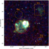 |
Fig. 1 False color image (red: 0.2-0.7 keV, green: 0.7–1.1 keV, blue: 1.1–10 keV) of the SNR IC443 and SNR G189.6+03.3 obtained with eRASS:4 dataset. For each of the three images, we applied the adaptive smoothing algorithm of Ebeling et al. (2006) with a minimum significance of the signal of S /N = 3 and a maximum of S /N = 5. The minimum scale of smoothing is 1 pixel, while the maximum is 8 pixels. The scale of the colors has been particularly stretched to highlight the diffuse emission. In orange, we display the extraction regions employed for the spectral analysis. The red circle is not used for spectral analysis purposes and is simply indicative of the suggested extension of G189.6+03.3 (the red cross marks the center of the circle at RA:06h19m40.8s, Dec:+21:58:03). The magenta cross indicates the center of IC443 at RA:06h17m0s and Dec:+22:34:00. |
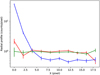 |
Fig. 2 Radial profiles extracted from the light blue circle region in Fig. 3 (red), from a region of the same size located inside G189.6+03.3 (green), and from another region centered on the star V398 Gem (blue), respectively. |
4 Spectral analysis
We carried out our analysis of the X-ray spectra with PyXSPEC, the Python interface of XSPEC (Arnaud 1996), and the errors are expressed in 1σ confidence level. We employed the Cash statistics (Cash 1979), using the version implemented in XSPEC. The choice of using the ratio CSTAT/dof (dof = degree of freedom) to estimate the goodness of the fit is motivated by the fact that for a sufficient number of counts, the C statistic approaches the x2 statistic (Kaastra 2017). In order to estimate the errors in a robust way, we ran an MCMC (Monte Carlo Markov chain) code using the Python library emcee (Foreman-Mackey et al. 2013), running it for 40 000 steps. We considered only the last 2000 steps of the run in order to get the largest possible number of chains converged. We initialized our walkers with a Gaussian distribution centered on the best-fit parameters, employing logarithmically uniform priors on the model components, which were left free to vary during the run. One of the main advantages of this approach over the traditional fitting technique is the capability to probe the parameters space in greater depth (see e.g., van Dyk et al. 2001, for a description of the advantage of using an MCMC-based approach in X-ray astronomy). We extracted the spectra from the regions shown in Fig. 1. Before proceeding with the spectral analysis, we removed the point sources in both background and source regions.
We started modeling the background spectrum following the approach of Okon et al. (2021) and references therein. The background extraction region is indicated in Fig. 1. The model consists of one power-law component representing the cosmic X-ray background with a fixed slope of 1.4 and three collisional equilibrium thermal model (APEC, Smith et al. 2001) components, each one with fixed temperature and solar abundances, but a free normalization. The Local Hot Bubble is modeled with a temperature of 0.105 keV, while the Galactic Halo is described by the other two APEC models with kT = 0.658 keV and kT = 1.22 keV, respectively. We absorbed the Galactic halo and cosmic X-ray background components with the TBabs model (Wilms et al. 2000). Given this modeling, we determined the best-fitting background model, first running a fit on the background region. We then fitted the background best-fitting model and the source model to the spectrum of each one of the regions shown in orange in Fig. 1. As from Fig. 1 the background is not significantly variable across the regions, we fixed the shape of the background model, fitting only a global normalization parameter simultaneously with the source. As an additional test, we checked our results by employing another background region extracted a few degrees south of G189.6+03.3, obtaining the same results. The spectra are shown in Fig. 6.
Following the labeling in Fig. 1, we started fitting region “A” with a constant temperature plane parallel shock thermal model (VPSHOCK, Borkowski et al. 2001) absorbed with the model TBabs (Wilms et al. 2000). This region should contain only the contribution from G189.6+03.3. The goodness of the fit was not acceptable, and so we decided to add another thermal shock component (VPSHOCK) while simultaneously applying a velocity shift (VASHIFT) to the initial model. We were motivated by the fact that from Fig. 1 the inner region A appears to be surrounded by a brighter emission, which we analyzed separately as region “B”. With the two-component model, we assume one component represents the inner emission of the remnant and the other the emission from an expanding shell. In the expanding component (the one multiplied by the velocity shift), we left only O, Mg, Ne, and Fe as free abundances, assuming that these elements are those mainly enriched, and also given that these are associated to the brightest lines. In the same component, we froze the abundance values of C, N, Si, and S to zero in order to avoid excessive degeneracy with the parameters of the other component. In the rest component, we instead set C, N, O, Mg, Ne, Fe, Si, and S free to vary: this model definitely improves the fit statistic (see Table 1 for the goodness of fits). The abundances not mentioned above are left frozen at solar value.
As mentioned in Sect. 1, starting from Yamaguchi et al. (2009), recombination was clearly detected in the spectra of IC443 in several studies, while it was also found to be a relevant process in G189.6+03.3 (Yamauchi et al. 2020). Therefore, we also tested a recombining plasma model (VRNEI, Foster et al. 2017) as a second additive component. The abundances were set as in the double VPSHOCK model and the initial cooling temperature T0 was set frozen to 5 keV. We decided to make the same assumption as that made by Okon et al. (2021): in this way, the O-S elements are fully ionized in the initial condition. Looking at the spectra, no extra residuals appear when a two-component model is applied and the difference in the statistics (Tables 1 and 2) between two VPSHOCK models and a single VPSHOCK plus a recombination component (VRNEI) is minimal. The ionization timescale parameter in both models is close to 1012 cm−3, indicating the gas is close to ionization equilibrium. However, the column density is significantly higher in the double-VPSHOCK model. We tried to investigate this feature, freezing some parameters in the velocity-shifted VPSHOCK component to the same values as the same parameters in the VPSHOCK+VRNEI model. We found that the double-VPSHOCK retrieves a column density  that is compatible with
  obtained with VPSHOCK+VRNEI if the ionization timescale and velocity shift are set equal to the values found in the VPSHOCK of the recombination model. We tried to also add a black-body radiation model to model the faint emission from the inner part (10 km in diameter, distance of 1500 pc, temperature of 0.1 keV) but the fit did not improve significantly.
In region B, we analyzed the bright external part of G189.6+03.3 emission, which is possibly associated with a shell. We initially tested a single-VPSHOCK model, but the fit retrieved strong residuals. The spectra are again better described by a two-component shocked plasma. We use either a VPSHOCK or VRNEI as a second component, we always find a column density of ~4.0 × 1021 cm−2 with similar statistic values. If we use VPSHOCK as a second component on top of the first VPSHOCK, we find a first plasma component with a temperature of  , with the second component showing
  . From Table 1, the double VPSHOCK model provides a CSTAT/dof ratio of close to 1, making it the best fit of all the tests we carried out. Therefore, we find additional evidence in favor of our initial hypothesis: the hot 2.3 keV expanding component can be associated to an expanding shell, while the inner emission is cooler, with a temperature of 0.7 keV. In Sect. 3 we show how the northern part of G189.6+03.3 is coincident with a dust structure visible in WISE data: it seems therefore reasonable to argue that the enhancement in the temperature of the plasma might be due to compression of the shock against a denser medium. This would imply that G189.6+03.3 and the HII region S249 are at the same distance. We also observe that the ionization timescale in the 0.7 keV component for the double VPSHOCK model is 4 × 1011 cm s−3 while in VPSHOCK plus VRNEI this timescale is 3 × 1012 cm s−3. As the statistics improve for the double VPSHOCK, we propose that the plasma is hot and recently shocked in this region. The higher value of τ in the 0.7 keV component in region B compared to the other regions (Table 1 and 2) is probably a consequence of the recent interaction of the gas with the nearby HII region.
We then proceeded to analyze the emission from regions C and D in order to understand whether or not G189.6+03.3 and IC443 overlap in terms of their plasma emission, as initially proposed by Asaoka & Aschenbach (1994). Indeed, these two regions are those covering IC443. For regions C and D, we find a two-component model provides the best fit to the data, as in region B. As visible in Table 1, if VPSHOCK is employed as the second component, we detect a temperature of close to kT ~ 0.7 keV in both regions. Conversely, in region ‘C’, the fits retrieve considerably improved statistics when employing VRNEI as a second component, but do not show hints of the 0.7 keV component (Table 2). Moreover, the column density is also inconsistent with 4.0 × 1021 cm−2, a value found in several other regions. Region C also displays a considerably high expansion velocity, which is not detected in region D. However, a justification for this difference is that the shock has been slowed down by the interaction with a molecular cloud in region D (Cornett et al. 1977; Ustamujic et al. 2021a). Observing Fig. 1, the two regions have similar surface brightness, which is especially relatively high in region C. It is therefore possible that the dim 0.7 keV component is not resolved in the spectrum of this region. We tested this scenario, adding an APEC component to the models employed above. The idea behind this choice is that the material is contained by the molecular cloud, and is possibly reheated by the reverse shock generated by the shock wave impacting the molecular cloud itself. The results are shown in Table 3.
With the addition of the APEC model to the VRNEI+VPSHOCK model, we obtained an improved statistic (Δ CSTAT = 23) and the 0.7 keV component appears again. Considering that the double VPSHOCK description leads to considerably poorer statistics, our conclusion is that the relaxed material (APEC) detected here belongs to G189.6+03.3, while the VSHOCK+VRNEI component is the shocked emission coming from IC443. This confirms previous findings of recombination and overionized material from this region (Yamaguchi et al. 2009; Greco et al. 2018).
Looking at region D, we find the 0.7 keV component with an ionization timescale factor of the plasma of  , again providing strong evidence for a plasma close to ionization equilibrium with physical properties very similar to those found in the other regions. The very low speed detected is additional evidence in support of the hypothesis that this relaxed gas was probably slowed down in the past due to interaction with a nearby molecular cloud. We recall how τ = 1013 s cm−3 is assumed as the upper limit of the ionization timescale parameter, implying collisional equilibrium in the VPSHOCK model (Arnaud 1996; Borkowski et al. 1994, 2001).
In conclusion, in all the regions studied here, we find a plasma component of constant temperature kT = 0.7 keV, suggesting that the emission from G189.06+3.3 covers all the regions analyzed, including those whose emission is associated with IC443 (region C and region D).
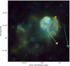 |
Fig. 3 Close up of Fig. 1 zoomed into IC443 and G189.6+03.3. The image is less stretched so as to better show the details within the remnant. The blue circle indicates the position of a putative central source in G189.6+03.3, and the transient is shown in orange (Identified with the source Gaia EDR3 3376739988615000320 and A11WISE J061853.77+214551.5). The green arrow indicates the proper motion direction of the pulsar B0611+22, while the light green arrow shows that of the fast-moving neutron star CXOU J061705.3+22212. Both arrows are obtained by multiplying the proper motion value by the age of each one of the compact objects. For illustrative purposes, the lengths of the arrows have been magnified ten times. The thin dotted yellow line highlights the elongated structure visible in eROSITA, while the orange thick line represents the jet direction suggested by Greco et al. (2018). |
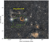 |
Fig. 4 Overplot of the X-ray contours obtained with eROSITA (light green) with the unWISE color archival data (W2, 4.6 μm; Wl, 3.4 μm). |
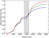 |
Fig. 5 Optical extinction in three different directions. Red: IC443. Green: G189.6+03.3. Blue: HII region S249. The dataset was obtained from the Gaw/2MASS extinction map available at https://astro,acri-st.fr/gaia_dev/. We also report the distance of 1.5 ± 0.2 pc adopted in the present paper (Fesen 1984; Welsh & Sallmen 2003). |
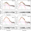 |
Fig. 6 Spectra from regions A, B, C, and D. The solid yellow line indicates the total model, the red dotted line represents the first additive component (VPSHOCK), and the red dashed line the second additive component (VPSHOCK). The dash dot lines show the different background components: the horizontal magenta line is the most significant component of the particle background, the others represent the sky background made by the Local Hot Bubble (dark green), cosmic X-ray background (violet), Cosmic Halo 1 (light violet), and Cosmic Halo 2 (light green). The spectra have been rebinned for better visualization and the parameters of the model are the median values of the last 2000 steps of the emcee run. |
Results from the spectral fits of the different regions using a double VPSHOCK model.
Results from the spectral fits of the different regions using a VPSHOCK plus VRNEI model.
Results from the spectral fits of region C using an additional APEC component on top of the model employed before.
4.1 An unresolved source at the center of G189.6+03.3?
Employing the best fit obtained above and despite the very few counts available, we modeled the emission of the diffuse emission close to the center of G189.6+03.3 described in Sect. 3. The spectra are background subtracted, except for the instrumental component, which we continued to model separately in order to describe the remaining high-energy tail. We first tested an unabsorbed POWERLAW with photon index fixed to 2 and free normalization to derive flux in the 0.2–10 keV band from the light-blue circle indicated in Fig. 3. We also left the column density free to vary, obtaining 0.33 × 1022 cm−2. The unabsorbed background subtracted flux is  . For the same region, we also tested the best-fit VPSHOCK+VRNEI model of region A (as discussed in Sect. 4, this has been proven to be more reliable than double VPSHOCK), obtaining an unabsorbed background-subtracted flux of
  . The spectrum is shown in Fig. 7. Despite the fact that we find a similar value for the CSTAT/DOF ratio (0.59) for both models, we find a considerably higher flux with the power-law model at 90% confidence level. Given its extended nature and the position almost at the center of G189.6+03.3, this object could be a pulsar wind nebula (PWN). Therefore, deeper observations with Chandra or XMM-Newton are needed to assess the nature of the object, considering that no radio detection is associated to this position.
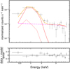 |
Fig. 7 Spectrum of the diffuse emission close to the center of G189.6+03.3 (light blue circle in Fig. 3) modeled with the VPSHOCK+VRNEI model. The data have been rebinned for visualization purposes. The two red lines indicate the two model components, while the magenta represents the instrumental background that we modeled. |
4.2 Two star clusters in the neighborhood
Thanks to the almost unlimited FOV of eROSITA provided by the all-sky scan survey mode, we were able to image two open clusters in the same sky region as IC443 and G189.6+03.3 (Fig. 1). These star clusters are NGC 2175 and NGC 2168 (also known as M35) and are indicated in Figs. 1 and 4, respectively.
Looking at the emission of M 35 above 0.7keV, it is in accordance with the presence of many hot and blue massive stars in the cluster (O,B spectral type). As many of these stars are massive, it is likely some could have already undergone a SN explosion. Strong winds and SN explosions from massive stars could have easily wiped out the dust, which is instead present around NGC 2175. A similar idea was proposed for the Galactic starburst cluster, Westerlund 1 (Muno et al. 2006; Clark et al. 2008; Negueruela et al. 2010). We extracted the spectrum of the diffuse emission around M35, masking the point sources. The spectrum appears to be relatively well (CSTAT/DOF = 1.07) described by a nonequilibrium shocked plasma (VPSHOCK model in XSPEC) with temperature kT = 0.15 ± 0.1 keV and  . In the fit, we left all the abundances free to vary, retrieving most of them as subsolar, except for Ne
  . The low value for the ionization timescale
  points towards a plasma out of equilibrium condition (see Sect. 4 for a discussion about this parameter). This is most likely due to collisionally shocked plasma essentially due to the strong winds coming from massive stars. However, we also consider the fact that this plasma is constantly illuminated by the same stars, and so photoionization effects should be important. Recently, Härer et al. (2023) discussed the importance of shocks in Westerlund 1 and in general for young star clusters in the context of TeV emission associated to Galactic cosmicray acceleration (see also Vieu & Reville 2023). The presence of shocked gas in our spectra of M 35 is in accordance with the turbulent environment needed to accelerate particles to TeV energies.
Moving to NGC 2175, a very faint diffuse emission can be observed in X-rays, which is found to be spatially coincident with a strong HII-emitting region visible in infrared (Fig. 4). We tried to extract the spectrum from the region indicated in Fig. 1, but we found it to be indistinguishable from the background. Additional observations are needed to provide a larger statistics with which to characterize the gas.
5 Discussion
In the previous Section, we show indications for the existence of a ubiquitous 0.7 keV plasma component present in all the regions analyzed. We find the column density is close to 4.0 × 1021 cm−2 in regions A, B, and D (only for the double VPSHOCK scenario). Some differences can arise between the two models in each region, resulting in slightly different absorption values, but the overall picture is a uniform absorber covering all the regions. For a detailed discussion of each region, see Sect. 4.
From these findings, we argue that the ubiquitous emission from the 0.7 keV plasma is associated with G189.6+03.3, which we find to be a foreground object, as first proposed by Asaoka & Aschenbach (1994), placed in front of IC443. In this context, the higher column density measured in region C when using a recombination model, together with high expansion velocity, might indicate that IC443 is a background object emerging from below G189.6+03.3. In addition, we clarified this aspect, adding another thermal component to the original model, again finding 0.7 keV. This shows that this component was not fitted with the previous model, probably because it is too dim, but it is there. This supports the idea that G189.6+03.3 is in front of IC443.
Ustamujic et al. (2021a) describe how the actual shape of IC443 might be the result of an interaction with two molecular clouds. Specifically, Fig. 3 of Ustamujic et al. (2021a) nicely fits the scenario in which IC443 is emerging from below an absorber. Moreover, from recent optical/UV data, Ritchey et al. (2020) propose that the star HD 254755 may be absorbed by material in the foreground that is possibly associated with G189.6+03.3. However, while Asaoka & Aschenbach (1994) initially proposed only a part of G189.6+03.3 is overlapping with IC443, our dataset suggests this may not be true, especially given that we detect an almost uniform column density. Our spectral analysis suggests instead that G189.6+03.3 is present in all the regions analyzed, including those associated with IC443 (C,D). In Fig. 1, we draw a red circle surrounding G189.6+03.3 in order to highlight this hypothesis (its center is shown as a red cross in Fig. 3). Moreover, Greco et al. (2018) recently showed that part of our region D is a shock ejecta and its shape can be correlated with the direction of the proper motion of the fast-moving neutron star to the south: these authors conclude that this structure belongs to IC443 and that the plasma is overionized. The same authors propose that the structure could be associated with a jet feature, as we indicate in Fig. 3. In the same figure, we also observe that, in the eROSITA image, G189.6+03.3 stretches from west to east. It is possible that two jet activities took place. The direction of the first is indicated with a yellow line in Fig. 3, which interestingly crosses the putative position of the unresolved source inside G189.6+03.3: this jet should be associated with the progenitor of G189.6+03.3 with its W part not visible due the very intense emission from IC443. The second jet structure is the one investigated by Greco et al. (2018) and should be related to IC443.
Starting from this interesting jet scenario, we want to figure out the possible types of progenitors. According to Smartt (2009), the progenitors with jets are very massive stars with M > 30 M⊙, specifically luminous blue variable (LBV) stars. However, recent papers, such as Chiotellis et al. (2021) and Ustamujic et al. (2021b), demonstrated the influence of massive progenitors in shaping the circumstellar medium (CSM) through the action of winds. The final effect can be an elongated shape similar to what is expected to be created by a jet and enriched ejecta. From our observation, we find supersolar abundances for O, Ne, Mg, and Si in the 0.7 keV plasma component. These abundances are close to what is described in Ustamujic et al. (2021b) for an LBV case. Contrary to what is predicted by this model, we detect subsolar iron abundances, but this can be easily explained by a poor modeling of the Fe L-shell lines, which are not resolved in eROSITA. Moreover, the effective area of eROSITA strongly decreases above 2 keV, making it almost unsuitable for observation of the strong Fe lines expected to arise from iron-rich ejecta. Nevertheless, the faint SN explosion model presents many of the features we highlight above. Specifically, these kinds of SNe are predicted to have high abundance ratios in the range [C/Fe]-[Al/Fe] as a consequence of a high amount of fallback material (Nomoto et al. 2013) and a jet-like structure. We indeed observe an elongated structure stretching from SE to NW in Fig. 3. We therefore evaluated the ratios between the abundances of O, Ne, Mg and S with the abundance of Si for each region. Ideally, we would have employed Fe, but given that it is almost not resolved in our data, we decided to employ Si, which is the element produced immediately before Fe during the explosion of a massive star. We show the results in Figs. 8 and 9. We observe that the ratio is above 1 for O, Ne, and Mg in several regions analyzed, as predicted with Fe in faint SNe for both the models tested.
Above we consider only single-star explosion models from core-collapse SNe; nevertheless, most of the stars are in binary systems. This is especially true for massive stars, which are likely to be born in crowded gas-rich areas of the Galaxy. Therefore, SN explosions are commonly driven by binary interaction (for a recent discussion, see Laplace et al. 2021). In Sect. 4, we show how the enhancement of the temperature of the plasma in region B might indicate that G189.6+03.3 is interacting with the HII region S249, especially looking at Fig. 4. As it is well known that IC443 is also interacting with this region (Fesen 1984; Ambrocio-Cruz et al. 2017), this suggests the two remnants are interacting with the same HII region, which would imply they are at the same distance, regardless of whether or not the progenitor is in a single or binary system. This would also be consistent with observing similar optical extinction measurement values in different points of the region, as described in Sect. 3. To test this scenario, we decided to assume a common distance (d = 1500 pc) for the two remnants and estimate the velocity of a hypothetical compact object associated to G189.6+03.3. As an explosion site, we consider the center of the red circle (RA:06h18m37.3s, Dec:+22:14:41.3) in Fig. 1 and shown as a red cross in Fig. 3. We took the coordinates of the diffuse emission (RA:06h19m40.8s, Dec:+21:58:03) described in Sect. 4.1 and visible in Fig. 3 as the current position of the object. Assuming 30 kyr as the time of explosion, the resulting velocity is around 315 km s−1. This value could be tested in the future with dedicated pointed observation on the bright spot. Assuming the same explosion site for J061705.3+22212, the fast-moving neutron star located close to the center of IC443, but assuming 3 kyr as the age and today’s position, we obtain a velocity of 3200 km s−1. Considering that the typical proper motion values found for other compact objects by Mayer & Becker (2021) are on average much lower than 3000 km s−1, we argue that an alternative mechanism to a simple natal kick from the SN explosion should be in place. The mechanism we propose to justify this very high proper motion value is a slingshot effect. Given the evidence provided for the existence of two separate remnants, it is appealing to consider a progenitor hosted in a system with three or more stars. Different works (see e.g., Thompson 2011; Naoz 2016; Hamers et al. 2022) have shown how the trajectories of the stars in such systems can be severely altered by the presence of a third star. The effect is even more chaotic when more stars are considered. Therefore, a slingshot effect might be a suitable explanation for finding one progenitor star very far from the other and a compact object with a very high proper motion value.
The slingshot mechanism would also explain why the proper motion of J061705.3+2221 is not aligned with the center of IC443 (Swartz et al. 2015; Greco et al. 2018), nor with the center of G189.6+03.3. Moreover, as shown by Ustamujic et al. (2021a), the center of the emission of IC443 determined by the maximum intensity of the X-ray emission is probably the result of complex interplay between the expanding shock wave and a molecular cloud. Therefore, it is likely that the direction of the compact object is not aligned with it. Having two SN explosions in two different regions would explain why the column density in region C is different from those measured in the other regions. However, it is also possible that two single stars belonging to the same association of stars – namely Gem OB1 – originated IC443 and G189.6+03.3, respectively. In this respect, the simulations of Ustamujic et al. (2021a) show how the single-explosion scenario could also explain the observed shape of IC443.
We also want to discuss how several papers (Yamaguchi et al. 2009; Matsumura et al. 2017) have demonstrated the presence of recombining plasma in the region of IC443. We also obtain good fits with such a model superimposed over shocked material. Interestingly, Yamauchi et al. (2020) detect a two-component recombining plasma in the northeast spot of G189.6+03.3 with Suzaku, one of which has a temperature of 0.7 keV. It is remarkable that values close to this temperature can also be found in all of the regions we tested and this is even more remarkable for region D, which is relatively far from the spot observed by Yamauchi et al. (2020). Comparing with Yamauchi et al. (2020), in this region, we find an ionization timescale of the same order of magnitude with the VPSHOCK+VRNEI model, but with poorer fit statistics compared to our double-VPSHOCK model. To explain this difference, we note how Tanaka et al. (2022) recently underlined the contribution that charge exchange can have in SNR X-ray spectra. To highlight this effect, the authors employ high-resolution spectra, which have a resolving power that our instrument cannot reach. Therefore, differences in the composition and density between the clouds in regions B and D might actually result in different contributions of charge exchange that cannot be resolved in our spectra. As charge exchange is likely to occur at the contact point between shock front and neutral material, this might explain the difference between our fit and those presented by Yamauchi et al. (2020). Nevertheless, considering that eROSITA is more sensitive to soft X-rays and instead Suzaku collects more photons in hard X-rays, the results can be considered relatively consistent among themselves.
In the same area of the sky, there are also two different compact objects. We tried to understand whether or not these could be associated with IC443 and G189.6+03.3. Starting from J061705.3+22212, the column density of 0.7 × 1021 cm−2 reported in Greco et al. (2018) is similar to what we obtain in region C (Sect. 4). Therefore, the most straightforward conclusion is that J061705.3+22212 is probably associated with IC443, as shown by many previous studies (Keohane et al. 1997; Swartz et al. 2015; Greco et al. 2018). Regarding the pulsar PSR B0611+22, the proper motion direction completely rules out the possibility that this object is correlated with G189.6+03.3 or with IC443. This is despite the fact that the column density derived in Sect. 3 is consistent with the column density measured for G189.6+03.3 (~4.0 × 1021 cm−2). This would imply that the source is at least as distant as the remnants, which does not exclude the possibility that PSR B0611+22 is located much farther away, as indicated from some models of dispersion measure. Therefore, given the proper motion direction and the great uncertainties in the dispersion measure models, it is less speculative to assume that this pulsar is not associated with either of the two SNRs.
In addition to these two compact objects, Bykov et al. (2008) and Zhang et al. (2018) showed the presence of several point sources at the eastern boundary of our region C thanks to deep Chandra, XMM-Newton, and NuSTAR observations. The nature of these objects is still unclear, especially given that at least two of them are found to be variable. Moreover, we observe that one of these objects (dubbed “srcla” in Bykov et al. 2008) appears to be a neutron star embedded in a pulsar wind nebula. Further studies are needed to assess whether it can be associated with IC443orG189.6+03.3.
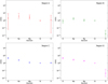 |
Fig. 8 Logarithmic ratio of the X element (O, Ne, Mg, Si, S) abundances with that of Si. The abundances are derived from a two-component fit employing two shock models (VPSHOCK). |
6 Conclusions
In this work, we finally confirm that G189.6+03.3 is a SNR. We find its emission can be represented by a two-thermal-component plasma, one of which is represented by a 0.7 keV temperature gas in equilibrium, which is found in all the regions analyzed. If we also consider that we detect a uniform absorption over the entire remnant close to ~4.0 × 1021 cm−2, we can argue that a unique diffuse emission covers the whole system. The high surface brightness of region C (Fig. 1) complicated the detection of the covering 0.7 keV component, which we manage to find by adding an additional APEC component to our models. Given the ubiquitous presence of this plasma at equilibrium, we conclude that G189.6+03.3 completely overlaps with IC443.
We obtain high abundance ratios of [O/Si], [Ne/Si], and [Mg/Si] in most of the regions and an elongated structure, which are all indications in favor of a faint SN explosion. From observing an enhancement of the temperature in the second plasma component of region B, we consider the possibility that G189.6+03.3 is interacting with the HII region S249, which is what IC443 appears to be doing. In this case, the two remnants should be placed at the same distance, presenting two possibilities: in one scenario, two isolated massive stars belonging to the group Gem OB1 generated the two remnants. An alternative and intriguing scenario is that, instead, it is two objects belonging to a multiple system that generated the two remnants.
Given these two hypotheses, we discuss the association with the remnants of the two nearby compact objects, confirming that CXOU J061705.3+22212 can be associated with IC443, while the pulsar PSR B0611+22 is unrelated to any of the two remnants. However, we suggest a third compact object could be in the field, seen as unresolved faint emission near the center of G189.6+03.3 (Sect. 4.1). Nevertheless, we also report how several unidentified point sources were observed in the past in the eastern part of IC443 and how it may also be possible that one of them is a compact object associated to one of the two remnants.
In conclusion, given the large number of new features shown in this work, we underline the necessity for new pointed observations of G189.6+03.3. A pointed observation toward the center would provide the means to assess the existence of a compact object, helping us to shed light on whether the progenitor was indeed a faint SN or the explosion happened via a different channel.
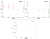 |
Fig. 9 Logarithmic ratio of the X element (O, Ne, Mg, Si, S) abundances with that of Si. The abundances are derived from a two-component fit employing one single temperature parallel shock model (VPSHOCK) and a recombination additive model (VRNEI). We do not show the plot for region C because the 0.7 keV component is absent when VRNEI is employed. |
Acknowledgements
We thank the anonymous referee for the useful comments and suggestions that helped to improve the quality of the manuscript. We would like to thank all the eROSITA team for the helpful discussions and suggestions provided during the realization of the paper. The image in Fig. 4 has been extracted with Aladin Desktop (Bonnarel et al. 2000) tool and replotted using astropy. F.C. acknowledges support from the Deutsche Forschungsgemeinschaft through the grant BE 1649/11-1 and from the International Max-Planck Research School on Astrophysics at the Ludwig-Maximilians University (IMPRS). F.C. thanks Hans-Thomas Janka for the useful discussion about SN explosion models and abundance yields. W.B. thanks James Turner for pointing out the observation of the source location of CXCO J061705.3+22212 in the FAST GPPS. This work is based on data from eROSITA, the soft X-ray instrument aboard SRG, a joint Russian-German science mission supported by the Russian Space Agency (Roskosmos), in the interests of the Russian Academy of Sciences represented by its Space Research Institute (IKI), and the Deutsches Zentrum für Luft- und Raumfahrt (DLR). The SRG spacecraft was built by Lavochkin Association (NPOL) and its subcontractors, and is operated by NPOL with support from the Max Planck Institute for Extraterrestrial Physics (MPE). The development and construction of the eROSITA X-ray instrument was led by MPE, with contributions from the Dr. Karl Remeis Observatory Bamberg & ECAP (FAU Erlangen-Nuernberg), the University of Hamburg Observatory, the Leibniz Institute for Astrophysics Potsdam (AIP) and the Institute for Astronomy and Astrophysics of the University of Tübingen, with the support of DLR and the Max Planck Society. The Argelander Institute for Astronomy of the University of Bonn and the Ludwig Maximilians Universität Munich also participated in the science preparation for eROSITA. The eROSITA data shown here were processed using the eSASS software system developed by the German eROSITA consortium. This work makes use of the Astropy Python package (https://www.astropy.org/, Astropy Collaboration 2013, 2018). A particular mention goes to the in-development coordinated package of Astropy for region handling called Regions (https://github.com/astropy/regions). We acknowledge also the use of Python packages Matplotlib (Hunter 2007), PyLaTex (https://github.com/JelteF/PyLaTeX/) and NumPy (Harris et al. 2020).
References
- Ambrocio-Cruz, P., Rosado, M., de la Fuente, E., Silva, R., & Blanco-Piñon, A. 2017, MNRAS, 472, 51 [NASA ADS] [CrossRef] [Google Scholar]
- Arnaud, K. A. 1996, ASP Conf. Ser., 101, 17 [Google Scholar]
- Asaoka, I., & Aschenbach, B. 1994, A&A, 284, 573 [NASA ADS] [Google Scholar]
- Astropy Collaboration (Robitaille, T. P., et al.) 2013, A&A, 558, A33 [NASA ADS] [CrossRef] [EDP Sciences] [Google Scholar]
- Astropy Collaboration (Price-Whelan, A. M., et al.) 2018, AJ, 156, 123 [Google Scholar]
- Bocchino, F., & Bykov, A. M. 2001, A&A, 376, 248 [NASA ADS] [CrossRef] [EDP Sciences] [Google Scholar]
- Bonnarel, F., Fernique, P., Bienaymé, O., et al. 2000, A&AS, 143, 33 [NASA ADS] [CrossRef] [EDP Sciences] [Google Scholar]
- Borkowski, K. J., Sarazin, C. L., & Blondin, J. M. 1994, ApJ, 429, 710 [NASA ADS] [CrossRef] [Google Scholar]
- Borkowski, K. J., Lyerly, W. J., & Reynolds, S. P. 2001, ApJ, 548, 820 [Google Scholar]
- Braun, R., & Strom, R. G. 1986, A&A, 164, 193 [NASA ADS] [Google Scholar]
- Brunner, H., Liu, T., Lamer, G., et al. 2022, A&A, 661, A1 [NASA ADS] [CrossRef] [EDP Sciences] [Google Scholar]
- Burton, M. G., Geballe, T. R., Brand, P. W. J. L., & Webster, A. S. 1988, MNRAS, 231, 617 [NASA ADS] [Google Scholar]
- Bykov, A. M., Krassilchtchikov, A. M., Uvarov, Y. A., et al. 2008, ApJ, 676, 1050 [NASA ADS] [CrossRef] [Google Scholar]
- Cash, W. 1979, ApJ, 228, 939 [Google Scholar]
- Chiotellis, A., Boumis, P., & Spetsieri, Z. T. 2021, MNRAS, 502, 176 [NASA ADS] [CrossRef] [Google Scholar]
- Clark, J. S., Muno, M. P., Negueruela, I., et al. 2008, A&A, 477, 147 [NASA ADS] [CrossRef] [EDP Sciences] [Google Scholar]
- Claussen, M. J., Frail, D. A., Goss, W. M., & Gaume, R. A. 1997, ApJ, 489, 143 [NASA ADS] [CrossRef] [Google Scholar]
- Cornett, R. H., Chin, G., & Knapp, G. R. 1977, A&A, 54, 889 [NASA ADS] [Google Scholar]
- Davies, J. G., Lyne, A. G., & Seiradakis, J. H. 1972, Nature, 240, 229 [NASA ADS] [CrossRef] [Google Scholar]
- Denoyer, L. K. 1978, MNRAS, 183, 187 [NASA ADS] [CrossRef] [Google Scholar]
- Ebeling, H., White, D. A., & Rangarajan, F. V. N. 2006, MNRAS, 368, 65 [NASA ADS] [Google Scholar]
- Fesen, R. A. 1984, ApJ, 281, 658 [NASA ADS] [CrossRef] [Google Scholar]
- Fesen, R. A., & Kirshner, R. P. 1980, ApJ, 242, 1023 [NASA ADS] [CrossRef] [Google Scholar]
- Foreman-Mackey, D., Hogg, D. W., Lang, D., & Goodman, J. 2013, PASP, 125, 306 [Google Scholar]
- Foster, A. R., Smith, R. K., & Brickhouse, N. S. 2017, AIP Conf. Ser., 1811, 190005 [Google Scholar]
- Gaensler, B. M., Chatterjee, S., Slane, P. O., et al. 2006, ApJ, 648, 1037 [NASA ADS] [CrossRef] [Google Scholar]
- Greco, E., Miceli, M., Orlando, S., et al. 2018, A&A, 615, A157 [NASA ADS] [CrossRef] [EDP Sciences] [Google Scholar]
- Grichener, A., & Soker, N. 2017, MNRAS, 468, 1226 [NASA ADS] [CrossRef] [Google Scholar]
- Hamers, A. S., Glanz, H., & Neunteufel, P. 2022, ApJS, 259, 25 [NASA ADS] [CrossRef] [Google Scholar]
- Han, J. L., Wang, C., Wang, P. F., et al. 2021, Res. Astron. Astrophys., 21, 107 [CrossRef] [Google Scholar]
- Härer, L. K., Reville, B., Hinton, J., Mohrmann, L., & Vieu, T. 2023, A&A, 671, A4 [NASA ADS] [CrossRef] [EDP Sciences] [Google Scholar]
- Harris, C. R., Millman, K. J., van der Walt, S. J., et al. 2020, Nature, 585, 357 [NASA ADS] [CrossRef] [Google Scholar]
- He, C., Ng, C. Y., & Kaspi, V. M. 2013, ApJ, 768, 64 [NASA ADS] [CrossRef] [Google Scholar]
- Humphreys, R. M. 1978, ApJS, 38, 309 [NASA ADS] [CrossRef] [Google Scholar]
- Hunter, J. D. 2007, Comput. Sci. Eng., 9, 90 [NASA ADS] [CrossRef] [Google Scholar]
- Kaastra, J. S. 2017, A&A, 605, A51 [NASA ADS] [CrossRef] [EDP Sciences] [Google Scholar]
- Keohane, J. W., Petre, R., Gotthelf, E. V., Ozaki, M., & Koyama, K. 1997, ApJ, 484, 350 [NASA ADS] [CrossRef] [Google Scholar]
- Lallement, R., Babusiaux, C., Vergely, J. L., et al. 2019, A&A, 625, A135 [NASA ADS] [CrossRef] [EDP Sciences] [Google Scholar]
- Laplace, E., Justham, S., Renzo, M., et al. 2021, A&A, 656, A58 [NASA ADS] [CrossRef] [EDP Sciences] [Google Scholar]
- Leahy, D. A. 2004, AJ, 127, 2277 [NASA ADS] [CrossRef] [Google Scholar]
- Manchester, R. N., Hobbs, G. B., Teoh, A., & Hobbs, M. 2005, AJ, 129, 1993 [Google Scholar]
- Matsumura, H., Tanaka, T., Uchida, H., Okon, H., & Tsuru, T. G. 2017, ApJ, 851, 73 [NASA ADS] [CrossRef] [Google Scholar]
- Mayer, M. G. F., & Becker, W. 2021, A&A, 651, A40 [NASA ADS] [CrossRef] [EDP Sciences] [Google Scholar]
- Medan, I., Lépine, S., & Hartman, Z. 2021, AJ, 161, 234 [NASA ADS] [CrossRef] [Google Scholar]
- Micelotta, E. R., Dwek, E., & Slavin, J. D. 2016, A&A, 590, A65 [NASA ADS] [CrossRef] [EDP Sciences] [Google Scholar]
- Mitsuda, K., Bautz, M., Inoue, H., et al. 2007, PASJ, 59, S1 [NASA ADS] [CrossRef] [Google Scholar]
- Muno, M. P., Law, C., Clark, J. S., et al. 2006, ApJ, 650, 203 [NASA ADS] [CrossRef] [Google Scholar]
- Naoz, S. 2016, ARA&A, 54, 441 [Google Scholar]
- Negueruela, I., Clark, J. S., & Ritchie, B. W. 2010, A&A, 516, A78 [NASA ADS] [CrossRef] [EDP Sciences] [Google Scholar]
- Nomoto, K., Kobayashi, C., & Tominaga, N. 2013, ARA&A, 51, 457 [CrossRef] [Google Scholar]
- Okon, H., Tanaka, T., Uchida, H., et al. 2021, ApJ, 921, 99 [NASA ADS] [CrossRef] [Google Scholar]
- Olbert, C. M., Clearfield, C. R., Williams, N. E., Keohane, J. W., & Frail, D. A. 2001, ApJ, 554, L205 [NASA ADS] [CrossRef] [Google Scholar]
- Predehl, P., & Schmitt, J. H. M. M. 1995, A&A, 500, 459 [Google Scholar]
- Predehl, P., Andritschke, R., Arefiev, V., et al. 2021, A&A, 647, A1 [EDP Sciences] [Google Scholar]
- Ritchey, A. M., Jenkins, E. B., Federman, S. R., et al. 2020, ApJ, 897, 83 [NASA ADS] [CrossRef] [Google Scholar]
- Salvato, M., Wolf, J., Dwelly, T., et al. 2022, A&A, 661, A3 [NASA ADS] [CrossRef] [EDP Sciences] [Google Scholar]
- Smartt, S. J. 2009, ARA&A, 47, 63 [NASA ADS] [CrossRef] [Google Scholar]
- Smith, R. K., Brickhouse, N. S., Liedahl, D. A., & Raymond, J. C. 2001, ApJ, 556, L91 [Google Scholar]
- Sunyaev, R., Arefiev, V., Babyshkin, V., et al. 2021, A&A, 656, A132 [NASA ADS] [CrossRef] [EDP Sciences] [Google Scholar]
- Swartz, D. A., Pavlov, G. G., Clarke, T., et al. 2015, ApJ, 808, 84 [NASA ADS] [CrossRef] [Google Scholar]
- Tanaka, Y., Uchida, H., Tanaka, T., et al. 2022, ApJ, 933, 101 [NASA ADS] [CrossRef] [Google Scholar]
- Thompson, T. A. 2011, ApJ, 741, 82 [NASA ADS] [CrossRef] [Google Scholar]
- Troja, E., Bocchino, F., & Reale, F. 2006, ApJ, 649, 258 [NASA ADS] [CrossRef] [Google Scholar]
- Troja, E., Bocchino, F., Miceli, M., & Reale, F. 2008, A&A, 485, 777 [NASA ADS] [CrossRef] [EDP Sciences] [Google Scholar]
- Ustamujic, S., Orlando, S., Greco, E., et al. 2021a, A&A, 649, A14 [NASA ADS] [CrossRef] [EDP Sciences] [Google Scholar]
- Ustamujic, S., Orlando, S., Miceli, M., et al. 2021b, A&A, 654, A167 [NASA ADS] [CrossRef] [EDP Sciences] [Google Scholar]
- van Dyk, D. A., Connors, A., Kashyap, V. L., & Siemiginowska, A. 2001, ApJ, 548, 224 [NASA ADS] [CrossRef] [Google Scholar]
- Vieu, T., & Reville, B. 2023, MNRAS, 519, 136 [Google Scholar]
- Welsh, B. Y., & Sallmen, S. 2003, A&A, 408, 545 [NASA ADS] [CrossRef] [EDP Sciences] [Google Scholar]
- Wilms, J., Allen, A., & McCray, R. 2000, ApJ, 542, 914 [Google Scholar]
- Yamaguchi, H., Ozawa, M., Koyama, K., et al. 2009, ApJ, 705, L6 [NASA ADS] [CrossRef] [Google Scholar]
- Yamauchi, S., Oya, M., Nobukawa, K. K., & Pannuti, T. G. 2020, PASJ, 72, 81 [NASA ADS] [CrossRef] [Google Scholar]
- Yao, J. M., Manchester, R. N., & Wang, N. 2017, ApJ, 835, 29 [NASA ADS] [CrossRef] [Google Scholar]
- Zhang, S., Tang, X., Zhang, X., et al. 2018, ApJ, 859, 141 [NASA ADS] [CrossRef] [Google Scholar]
- Zhong, J., Li, J., Carlin, J. L., et al. 2019, ApJS, 244, 8 [NASA ADS] [CrossRef] [Google Scholar]
- Zhu, H., Slane, P., Raymond, J., & Tian, W. W. 2019, ApJ, 882, 135 [NASA ADS] [CrossRef] [Google Scholar]
The software version is denoted according to the date when it was released, i.e. 14.12.2021.
The Five-hundred-meter Aperture Spherical radio Telescope (FAST) Galactic Plane Pulsar Snapshot http://zmtt.bao.ac.cn/GPPS/GPPSnewPSR.html
All Tables
Results from the spectral fits of the different regions using a double VPSHOCK model.
Results from the spectral fits of the different regions using a VPSHOCK plus VRNEI model.
Results from the spectral fits of region C using an additional APEC component on top of the model employed before.
All Figures
|
Fig. 1 False color image (red: 0.2-0.7 keV, green: 0.7–1.1 keV, blue: 1.1–10 keV) of the SNR IC443 and SNR G189.6+03.3 obtained with eRASS:4 dataset. For each of the three images, we applied the adaptive smoothing algorithm of Ebeling et al. (2006) with a minimum significance of the signal of S /N = 3 and a maximum of S /N = 5. The minimum scale of smoothing is 1 pixel, while the maximum is 8 pixels. The scale of the colors has been particularly stretched to highlight the diffuse emission. In orange, we display the extraction regions employed for the spectral analysis. The red circle is not used for spectral analysis purposes and is simply indicative of the suggested extension of G189.6+03.3 (the red cross marks the center of the circle at RA:06h19m40.8s, Dec:+21:58:03). The magenta cross indicates the center of IC443 at RA:06h17m0s and Dec:+22:34:00. |
| In the text | |
|
Fig. 2 Radial profiles extracted from the light blue circle region in Fig. 3 (red), from a region of the same size located inside G189.6+03.3 (green), and from another region centered on the star V398 Gem (blue), respectively. |
| In the text | |
|
Fig. 3 Close up of Fig. 1 zoomed into IC443 and G189.6+03.3. The image is less stretched so as to better show the details within the remnant. The blue circle indicates the position of a putative central source in G189.6+03.3, and the transient is shown in orange (Identified with the source Gaia EDR3 3376739988615000320 and A11WISE J061853.77+214551.5). The green arrow indicates the proper motion direction of the pulsar B0611+22, while the light green arrow shows that of the fast-moving neutron star CXOU J061705.3+22212. Both arrows are obtained by multiplying the proper motion value by the age of each one of the compact objects. For illustrative purposes, the lengths of the arrows have been magnified ten times. The thin dotted yellow line highlights the elongated structure visible in eROSITA, while the orange thick line represents the jet direction suggested by Greco et al. (2018). |
| In the text | |
|
Fig. 4 Overplot of the X-ray contours obtained with eROSITA (light green) with the unWISE color archival data (W2, 4.6 μm; Wl, 3.4 μm). |
| In the text | |
|
Fig. 5 Optical extinction in three different directions. Red: IC443. Green: G189.6+03.3. Blue: HII region S249. The dataset was obtained from the Gaw/2MASS extinction map available at https://astro,acri-st.fr/gaia_dev/. We also report the distance of 1.5 ± 0.2 pc adopted in the present paper (Fesen 1984; Welsh & Sallmen 2003). |
| In the text | |
|
Fig. 6 Spectra from regions A, B, C, and D. The solid yellow line indicates the total model, the red dotted line represents the first additive component (VPSHOCK), and the red dashed line the second additive component (VPSHOCK). The dash dot lines show the different background components: the horizontal magenta line is the most significant component of the particle background, the others represent the sky background made by the Local Hot Bubble (dark green), cosmic X-ray background (violet), Cosmic Halo 1 (light violet), and Cosmic Halo 2 (light green). The spectra have been rebinned for better visualization and the parameters of the model are the median values of the last 2000 steps of the emcee run. |
| In the text | |
|
Fig. 7 Spectrum of the diffuse emission close to the center of G189.6+03.3 (light blue circle in Fig. 3) modeled with the VPSHOCK+VRNEI model. The data have been rebinned for visualization purposes. The two red lines indicate the two model components, while the magenta represents the instrumental background that we modeled. |
| In the text | |
|
Fig. 8 Logarithmic ratio of the X element (O, Ne, Mg, Si, S) abundances with that of Si. The abundances are derived from a two-component fit employing two shock models (VPSHOCK). |
| In the text | |
|
Fig. 9 Logarithmic ratio of the X element (O, Ne, Mg, Si, S) abundances with that of Si. The abundances are derived from a two-component fit employing one single temperature parallel shock model (VPSHOCK) and a recombination additive model (VRNEI). We do not show the plot for region C because the 0.7 keV component is absent when VRNEI is employed. |
| In the text | |
Current usage metrics show cumulative count of Article Views (full-text article views including HTML views, PDF and ePub downloads, according to the available data) and Abstracts Views on Vision4Press platform.
Data correspond to usage on the plateform after 2015. The current usage metrics is available 48-96 hours after online publication and is updated daily on week days.
Initial download of the metrics may take a while.