| Issue |
A&A
Volume 680, December 2023
|
|
|---|---|---|
| Article Number | A8 | |
| Number of page(s) | 14 | |
| Section | Planets and planetary systems | |
| DOI | https://doi.org/10.1051/0004-6361/202346840 | |
| Published online | 05 December 2023 | |
Photometric follow-up of the 20 Myr old multi-planet host star V1298 Tau with CHEOPS and ground-based telescopes★
1
INAF – Osservatorio Astrofisico di Torino,
Via Osservatorio 20,
10025
Pino Torinese, Italy
e-mail: This email address is being protected from spambots. You need JavaScript enabled to view it.
2
INAF – Osservatorio Astrofisico di Catania,
Via S. Sofia 78,
95123
Catania, Italy
3
INAF – Osservatorio Astronomico di Padova,
Vicolo dell’Osservatorio 5,
35122
Padova, Italy
4
Aix-Marseille Univ., CNRS, CNES, LAM,
Marseille, France
5
Department of Physics, University of Rome “Tor Vergata”,
Via della Ricerca Scientifica 1,
00133
Rome, Italy
6
Max Planck Institute for Astronomy,
Königstuhl 17,
69117
Heidelberg, Germany
7
Gruppo Astrofili Catanesi,
Via Milo 28,
95125
Catania, Italy
8
Stockholm University, Department of Astronomy AlbaNova University Center,
106 91
Stockholm, Sweden
9
INAF – Osservatorio Astronomico di Palermo,
Piazza del Parlamento 1,
90134
Palermo, Italy
10
Instituto de Astrofísica de Canarias (IAC),
Calle Vía Láctea s/n,
38200
La Laguna, Tenerife, Spain
11
Departamento de Astrofísica, Universidad de La Laguna (ULL),
38206
La Laguna, Tenerife, Spain
12
Dipartimento di Fisica e Chimica E. Segré, Università di Palermo,
Via Archirafi 36,
90100
Palermo, Italy
13
Dipartimento di Matematica e Fisica, Università Roma Tre,
Via della Vasca Navale 84,
00146
Roma, Italy
14
Centro de Astrobiología CSIC-INTA,
Carretera de Ajalvir km 4,
28850
Torrejón de Ardoz, Madrid, Spain
Received:
8
May
2023
Accepted:
22
September
2023
Abstract
Context. The 20 Myr old star V1298 Tau hosts at least four planets. Since its discovery, this system has been a target of intensive photometric and spectroscopic monitoring. To date, the characterisation of its architecture and planets’ fundamental properties has been very challenging.
Aims. The determination of the orbital ephemeris of the outermost planet V1298 Tau e remains an open question. Only two transits have been detected so far by Kepler/K2 and TESS, allowing for a grid of reference periods to be tested with new observations, without excluding the possibility of transit timing variations. Observing a third transit would allow for better constraints to be set on the orbital period and would also help in determining an accurate radius for V1298 Tau e because the previous transits showed different depths.
Methods. We observed V1298 Tau with the CHaracterising ExOPlanet Satellite (CHEOPS) to search for a third transit of planet e within observing windows selected to test three of the shortest predicted orbital periods. We also collected ground-based observations to verify the result found with CHEOPS. We reanalysed Kepler/K2 and TESS light curves to test how the results derived from these data are affected by alternative photometric extraction and detrending methods.
Results. We report the CHEOPS detection of a transit-like signal that could be attributed to V1298 Tau e. If so, that result would imply that the orbital period calculated from fitting a linear ephemeris to the three available transits is close to ~45 days. Results from the ground-based follow-up marginally support this possibility. We found that i) the transit observed by CHEOPS has a longer duration compared to that of the transits observed by Kepler/K2 and TESS; and ii) the transit observed by TESS is >30% deeper than that of Kepler/K2 and CHEOPS, and it is also deeper than the measurement previously reported in the literature, according to our reanalysis.
Conclusions. If the new transit detected by CHEOPS is found to be due to V1298 Tau e, this would imply that the planet experiences TTVs of a few hours, as deduced from three transits, as well as orbital precession, which would explain the longer duration of the transit compared to the Kepler/K2 and TESS signals. Another and a priori less likely possibility is that the newly detected transit belongs to a fifth planet with a longer orbital period than that of V1298 Tau e. Planning further photometric follow-up to search for additional transits is indeed necessary to solve the conundrum, as well as to pin down the radius of V1298 Tau e.
Key words: stars: individual: V1298 Tau / planetary systems / techniques: photometric
Based on data collected within the CHEOPS AO-3 proposal PR230032 Pinning down orbital period, transit ephemeris, and radius of the infant planet V1298 Tau e.
© The Authors 2023
 Open Access article, published by EDP Sciences, under the terms of the Creative Commons Attribution License (https://creativecommons.org/licenses/by/4.0), which permits unrestricted use, distribution, and reproduction in any medium, provided the original work is properly cited.
This article is published in open access under the Subscribe to Open model. This email address is being protected from spambots. You need JavaScript enabled to view it. to support open access publication.
1 Introduction
V1298 Tau (also known as K2-309) is a 20 ± 10 Myr-old K1 star of bolometric luminosity: L = 0.954 ± 0.040 L⊙; magnitude: V = 10.12 ± 0.05; distance: 109.5 ± 0.7 pc (Suárez Mascareño et al. 2021) that hosts four transiting planets discovered by Kepler/K2 (David et al. 2019a,b). This very young multi-planet system provides a unique opportunity to characterise planets at a very early phase after their formation. In turn, this allows us to constrain evolutionary models whose theoretical predictions remain untested to date due to the paucity of such systems detected so far. Right after the discovery, V1298 Tau became a target of intense multi-instrument, multi-band spectroscopic and photometric follow-up (Poppenhaeger et al. 2021; Feinstein et al. 2021; Suárez Mascareño et al. 2021; Vissapragada et al. 2021; Gaidos et al. 2022; Johnson et al. 2022). The study carried out by Suárez Mascareño et al. (2021) had the primary aim of measuring masses and bulk densities of the four planets in the V1298 Tau system through spectroscopic observations. Their results show that V1298 Tau b has a mass of 0.64 ± 0.19 MJup and a density similar to that of giant planets in the Solar System and other known old giant exoplanets. For the outermost V1298 Tau e, for which only one transit was detected at that time, Suárez Mascareño et al. (2021) determined an orbital period of Pe = 40.2 ± 0.1 days, a mass of 1.16 ± 0.30 MJup, and a density slightly larger, but compatible within error bars, than that of most of the older giant exoplanets. This unexpected result suggests that giant planets of such a young age might evolve and contract within the first million years after system’s birth, thus challenging current models of planetary formation and evolution. Following the results of Suárez Mascareño et al. (2021), Maggio et al. (2022) investigated the current escape rates from the planetary atmospheres and predicted the future evolution of atmospheric photo-evaporation, while Tejada Arevalo et al. (2022) investigated stability constraints on the system’s orbital architecture.
Despite a first and demanding follow-up, the results by Suárez Mascareño et al. (2021) and their implications need to be confirmed; thus, an accurate characterisation of the V1298 Tau system remains an open issue and a hot topic. In September–October 2021 the Transiting Exoplanet Survey Satellite (TESS) observed V1298 Tau and detected a second transit attributed to planet e, as reported by Feinstein et al. (2022). They constrained the orbital period of the outermost planet to a grid of discrete values (i.e. Pe > 44 days, which is not in agreement with the result found by Suárez Mascareño et al. 2021 through spectroscopy) that is the only reasonable calculation when just two transits are detected. The discrete periods in the grid have been determined by dividing, for integer numbers, the time separation between the epochs of central transit observed by Kepler/K2 and TESS, and they have to be interpreted as a guidance to search for future transits of planet e. These periods would correspond to actual values of Pe if there are no substantial changes in the orbital parameters over short time scales and without the presence of large transit timing variations (TTVs). The information currently available about the system does not allow us to reliably predict any significant orbital instability and an upcoming transit follow-up strategy must be necessarily based on the grid of orbital periods defined by Feinstein et al. (2022).
Feinstein et al. (2022) also showed that the transit depths of V1298 Tau bcd measured from TESS data are slightly shallower, but compatible within 1–2σ, than those observed by Kepler/K2, while the transit depth of V1298 Tau e is ~3σ larger. They conclude by proposing a few scenarios to qualitatively explain this discrepancy in radius measurements between Kepler/K2 and TESS, all of them involving phenomena that are not well characterised yet for systems with very young ages which make any interpretation very complex, going from the rapidly evolving stellar activity to haze-dominated planetary atmospheres. Sikora et al. (2023) presented a reanalysis of the spectroscopic and photometric data of V1298 Tau, including additional RVs to the dataset of Suárez Mascareño et al. (2021). Concerning V1298 Tau e, and with a reference to the grid of guidance orbital periods derived by Feinstein et al. (2022), Sikora et al. (2023) have concluded that periods of Pe > 55.4 days can be ruled out at 3σ level. Additionally, they placed a tight constraint on Pe (Pe = 46.768131 ± 0.000076 days, assuming a circular orbit, although the actual orbital architecture of V1298 Tau e remains unknown.
In order to improve the characterisation of this system, we carried out a follow-up study of V1298 Tau with the CHaracterising ExOPlanet Satellite (CHEOPS) space telescope (Benz et al. 2021). Our aim has been twofold1: i) detecting additional transits of planet e, providing better constraints to its orbital period, and a first identification of TTVs, with the consequent improvement of the results by Feinstein et al. (2022) and ii) getting a new measurement of its radius, possibly helping to explain the different transit depths measured from Kepler/K2 and TESS light curves (LCs). In this work, we present results from the CHEOPS monitoring conducted between 18 November and 18 December 2022, as well as from further ground-based photometric follow-up that was motivated by the outcomes of CHEOPS observations. We also reanalysed the TESS photometry that we extracted using an alternative pipeline to correct for contamination from nearby faint stars and we compare the results to those of Feinstein et al. (2022).
2 Description of the photometric data
2.1 Kepler/K2
We used the EVEREST 2.0 (Luger et al. 2018) version of the Kepler/K2 LC, which had been analysed by David et al. (2019b) and Feinstein et al. (2022). The time series covers about 71 days, from 8 February 2015 to 20 April 2015 (Kepler/K2 Campaign 4).
2.2 TESS
V1298 Tau was observed by TESS between 16 September and 6 November 2021 (Sectors 43 and 44), and the observations were analysed shortly after by Feinstein et al. (2022). We re-extracted the LC from the TESS Full Frame Images (FFIs) with the PATHOS pipeline described by Nardiello et al. (2019, 2020). First, we extracted the long-cadence LC (cadence of 10 min) by using six different photometric apertures (PSF-fitting, 1-px, 2-px, 3-px, 4-px, and 5-px radius aperture photometry) after subtracting from each FFI the sources within 3 arcmin from V1298 Tau. Then, we corrected the LC by applying the cotrending basis vectors (CBVs) calculated as in Nardiello et al. (2021). We selected the best photometric aperture comparing the point-to-point (P2P) rms of the different LCs, finding that the lower P2P rms is that associated with the PSF-fitting light curve. V1298 Tau is an ideal target to be analysed with the PATHOS pipeline, that was developed to extract high-precision light curves in crowded fields, like open clusters. The PSF-fitting photometry performed with empirical PSFs allow us to minimise the dilution effects due to the contamination of close-by stars (following the TIC catalogue, there are 63 sources within 3 arcmin, with 2 of them characterised by T ~ 9.6 and T ~ 7.9). Moreover, in Nardiello et al. (2022), we discuss the fact that our CBV correction of systematic errors in the light curves is expected to perform more effectively than other pipelines in the case of active stars such as V1298 Tau (no spurious signals or transit deformations were present in our final light curves).
 |
Fig. 1 Light curve of V1298 Tau collected on the night of 8 February 2022 with the Schmidt 67/92 cm telescope at the INAF-Astrophysical Observatory of Asiago. The red dots correspond to the binned light curve, and the green curve represents the transit model of planet e based on the ephemeris and transit depth derived by Feinstein et al. (2022). |
2.3 CHEOPS
We were awarded a total of 112 CHEOPS orbits to test three orbital periods of V1298 Tau e with the highest probability among those calculated by Feinstein et al. (2022) from the temporal separation between the two transits seen by Kepler/K2 and TESS, namely 44.1699, 45.0033, and 46.7681 (±0.0001) days. It must be emphasised that the grid of periods proposed by Feinstein et al. (2022) originates from just two observed transits and they can be used as a guidance to search for a third transit that would better constraint the orbital ephemeris. Our original plan was dividing the 112 orbits in six visits, two visits per test period, in order to collect two transits in the case of a successful detection and get a robust measurement of the orbital period and planet’s radius. In practice, three over six visits have been executed. We did not select P = 45.8687 days as a test period from the grid because only one CHEOPS visit could be accommodated in the available time span, due to observing constraints. Concerning this period, we did not find clear evidence for a transit event in photometry collected between BJDTDB 2459619.2380 and 2459619.4459 (8 February 2022), with the Schmidt 67/92 cm telescope at the INAF-Astrophysical Observatory of Asiago, when a transit was predicted with ingress, centre, and egress BJDTDB 2459619.24662, 2459619.40162, and 2459619.55662, respectively. This LC is shown in Fig. 1 and was extracted as described in Nardiello et al. (2015, 2016). Looking at the data, we cannot claim a detection with a significance better than nearly 2σ. Also, possible large TTVs should be taken into account before discarding P = 45.8687 days from the list of the possible guidance orbital periods. The TTVs cannot be reliably predicted yet because, as already mentioned, many critical information about the system are still missing. Nonetheless, we found convenient for the sake of our proposal to focus on the other three high-probability test periods that we selected. The observing windows have been centred to the predicted time of central transit assuming no TTVs, and their time span (nearly 1 or 2 days) has been defined to allocate to some extent possible, but still unknown TTVs.
We extracted the LC using the point spread function (PSF) photometry package PIPE2 (Brandeker et al. 2022), which is suitable for crowded fields. This pipeline models the background stars before extracting the photometry of the target by fitting a PSF. The PSF fitting is weighted by the signal and noise of each pixel, thus the extraction is less sensitive than aperture photometry to background star contamination. We use this curve in the present analysis. A comparison with the default data reduction pipeline (DRP) of CHEOPS (Hoyer et al. 2020) reveals a general 30% improvement in the overall photometric scatter. However, as a cross-check we also analysed the DRP photometry, finding no differences in the results within the uncertainties. For convenience, we show the bandpasses of the Kepler/K2, TESS and CHEOPS space telescopes in Fig. 2.
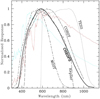 |
Fig. 2 Bandpasses of Kepler/K2, TESS, and CHEOPS normalised to their peak values, as a function of wavelength. The cyan and red curves represent the spectral energy distributions of a Teff = 5500 K and Teff = 4500 K dwarf star, respectively (image taken from https://www.cosmos.esa.int/web/cheops/performances-bandpass). |
2.4 Ground-based observations
V1298 Tau was observed during the night of 31 January-01 February 2023 by ground-based facilities in Italy and Spain. This joint follow-up was aimed to support the findings of CHEOPS described in Sect. 3, and the involved facilities are described in the following.
Asiago Copernico. We gathered a photometric series through a Sloan r filter with the AFOSC instrument (Asiago Faint Object Spectrograph and Camera) mounted at the 1.82-m Copernico telescope at Cima Ekar, in northern Italy3. A total of 3364 frames were collected with a constant exposure time of 5 s from 17:07 UT to 00:18 UT, when the target elevation went below the safety limit. The sky was mostly clear throughout the series with a few passing thin veils. The 81%-illuminated Moon at just 16° from the line of sight resulted in a very high background level and a scatter larger than usual, but with no significant impact on photometric accuracy. The images, purposely defocused to ~7″ FWHM to improve photometric accuracy and avoid saturation, were bias- and flat-field corrected using standard procedures. A LC was then extracted with the STARSKY code (Nascimbeni et al. 2013), a photometric pipeline developed by the TASTE project (Nascimbeni et al. 2011) to perform high-precision differential aperture photometry over defocused images.
Asiago Schmidt. We also acquired a photometric series through a Sloan i filter with a second telescope at the same observing site, the Asiago 67/92 cm Schmidt camera operating in robotic mode4. A total of 836 frames were collected with a constant exposure time of 7 s from 17:28 UT to 00:04 UT, with two ~ 30 min gaps in the first half due to technical issues. A differential LC was extracted using the same STARSKY procedure applied to the Asiago Copernico data.
Calar Alto. V1298 Tau was also observed with the Zeiss 1.23 m telescope at the observatory of Calar Alto (Spain), using a Cousins-I filter. We defocussed the telescope to improve the quality of the photometric data, a technique often used for transit follow-up (Southworth et al. 2009). We used unbinned and windowed CCD (DLR-MKIII CCD camera5, field of view 21.4′ × 21.4′) in order to decrease the saturation threshold and the readout time. The monitoring started on 31 January 2023 18:45 UT (airmass 1.06), and ended on 01 February 2023 00:24 UT (airmass 2.31). The exposure time was gradually increased from 30 to 75 s with the increase of the airmass. The images were reduced using master-flat and master bias frames which were collected before the scientific observations. The calibrated time series were corrected for pointing variations, and aperture differential photometry was performed with the APER routine, which is part of the IDL ASTROLIB library (Landsman 1993).
Catania. Photometric observations were collected with the 25-cm Newtonian telescope of Gruppo Astrofili Catanesi (Catania, Italy; lon. 15:05:32 E, lat. +37:30:23, alt. 42 m) using a Johnson-Cousins R filter. The telescope was equipped with a coma corrector and a CCD camera Sbig ST-7 XME. Overall, 243 frames were acquired from 17:37 UT to 00:33 UT with a constant exposure time of 100 s, chosen to reduce the effects of scintillation. To optimise the signal-to-noise ratio (S/N), a slight defocus was used, obtaining a FWHM of about 7″. After standard calibration of each image with bias, dark and flat field frames, the light curve was obtained via an un-weighted ensemble aperture photometry with the software AstroImage J (Collins et al. 2017).
3 Light curve modelling
We analysed the LCs of all instruments in a Bayesian framework. We used the python package SnappyKO (Parviainen & Korth 2020) to model the transits. Correlated signals due to stellar activity are modelled through a Gaussian process (GP) regression using the S+LEAF python library (Delisle et al. 2020, 2022). All the details of the GP modelling are provided in Appendix A.
The likelihood maximisation is performed with a Markov chain Monte Carlo (MCMC) using the package emcee version 3.1.3 (Foreman-Mackey et al. 2013), a python implementation of the affine invariant MCMC ensemble sampler by Goodman & Weare (2010). We ran the code in the HOTCAT computing infrastructure (Bertocco et al. 2020; Taffoni et al. 2020) to speed-up the computational time.
3.1 Kepler/K2 light curve
We masked the transits of planets bcd from the Kepler/K2 LC by computing the time of transits using the ephemeris of David et al. (2019b) and trimming a time window of 1.5 times the corresponding transit duration centred on the expected transit time. Then, we flattened the LC using the best-fit model of David et al. (2019b), in order to identify and reject stellar flares (using a +5σ clipping threshold above the best-fit model).
As discussed in Appendix A, we found that the best GP model is a combination of a quasi-periodic Exponentialsine periodic (ESP) kernel to trace the rotational signal and stochastically-driven harmonic oscillator (SHO) kernel to model the low-frequency correlated noise, which is likely of stellar origin, as it is recovered also in the analysis of the TESS LC (see Sect. 3.2).
We fit the data using a model containing simultaneously the transit signal of planet e (assuming a circular orbit) and the correlated stellar rotation signal. We used the priors listed in Table 1. For the orbital period Pe we used a uniform prior of 𝒰(35, 100) days and for the time of central transit, we used a uniform prior of 𝒰(2457096.46, 2457096.79) BJDTDB centred on the epoch of transit indicated by David et al. (2019b). We used the stellar density instead of fitting directly the scaled semi-major axis, a/R*, adopting a Gaussian prior based on the measurement of Suárez Mascareño et al. (2021). To fit the limb darkening (LD) coefficients (adopting a quadratic law), we used priors based on the results of David et al. (2019b). The Kepler/K2 LC has a cadence of 29.4 min. Following a common practice, in order to mitigate morphological distortions introduced when fitting transit light curves with such a long cadence (see e.g. Kipping 2010), we used an oversampling factor of 3. This means that each simulated photometric data point at the epoch of a real observation is calculated as the average value of three evenly spaced simulated data points each corresponding to a 10-min exposure.
We ran the markov chain monte carlo (MCMC) for 100 000 steps, which turned out to be ~150 times the auto-correlation length of the chains, estimated following Goodman & Weare (2010). This indicated successful convergence, as suggested by Sokal (1997) and adapted to parallel Monte Carlo chains6. The best-fit model of the Kepler/K2 LC is shown in Fig. 3, while in Fig. 4 we show the detrended transit signal (black dots). We obtained a transit best-fit solution consistent with David et al. (2019b) within 1σ (Table 1).
3.2 TESS light curve
For the fit of the TESS LC, we used the same approach adopted for the Kepler/K2 data, as described above. Also in this case, we found out that a mixture of a ESP and SHO kernels provides a more realistic representation of the correlated noise in the LC and through several tests, we found that using different kernels does not affect the transit parameters. Following the results of Feinstein et al. (2022), we used the prior 𝒰(2 459 481.63,2 459 481.96) BJDTDB for the time of transit and a Gaussian prior for the LD coefficients. We used an over-sampling factor of 3 to model the data with a cadence of 10 min. The best-fit model and the detrended transit signal are shown in Figs. 3 and 4 (orange dots), respectively. For comparison, we also show in Fig. 4 the TESS transit measured by Feinstein et al. (2022; green data points), which has a lower depth. This discrepancy is due to both the different LC extraction methods and GP regression analysis, as it is evident looking at Fig. C.1. The two LCs looks very similar, except for the out of transit segments and our GP-modelled flux is higher during the transit timespan, determining a deeper transit in our case overall.
Model parameters for the fit of the Kepler/K2 and TESS data.
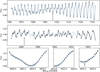 |
Fig. 3 Kepler/K2, TESS, and CHEOPS LCs of V 1298 Tau from top to bottom row, respectively. In each panel, the blue solid line shows the best-fit model. The arrows indicate the transits of the companion labelled as planet e by David et al. (2019b) and Feinstein et al. (2022), based on data from K2 and TESS. |
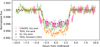 |
Fig. 4 Comparison of the detrended transit LCs discussed in this work as seen by Kepler/K2, TESS and CHEOPS. For each dataset, the best-fit transit model is shown by curves with the same colour as the data points. The green data points identify the detrended and flattened TESS light curve analysed by Feinstein et al. (2022), obtained from the jupyter notebook made publicly available by the authors online (https://github.com/afeinstein20/v1298tau_tess/blob/main/notebooks/TESS_V1298Tau.ipynb). |
3.3 CHEOPS light curve
We modelled the LC of all the CHEOPS visits using the same framework described above and taking advantage of some of the results from the previous analysis. First of all, we found that a simple undamped SHO kernel could effectively mitigate the correlated signal present in the LC that is due to the stellar rotation. This is expected from the fact that the Lomb-Scargle (LS) peri-odogram of the data shows only the rotational peak – and not its harmonics. Moreover, the adoption of the SHO kernel minimises the number of free parameters compared to the ESP kernel. We assumed that the low-frequency correlated noise detected in the Kepler/K2 and TESS data could not be recovered in CHEOPS data due to the limited time span and sparse sampling. Thus, we fit the GP correlated noise using a Gaussian prior for the stellar rotation frequency, vrot, measured in the TESS data (corresponding to the rotation period of ~2.9 days). For the LD coefficients, we used Gaussian priors based on the results of David et al. (2019b) because Kepler and CHEOPS passbands are similar (Fig. 2; and Benz et al. 2021). The prior on the time of inferior conjunction, T0, is uniform and spans the full extent of the CHEOPS follow-up (𝒰(2 459 901.8, 2459 932.5) BJDTDB) in order to keep the search for a transit signal blind. We adopted a uniform prior of 𝒰(35, 100) days for the orbital period of a possible transiting companion.
The CHEOPS LCs are affected by periodic instrumental noise due to the roll of the telescope. We modelled this systematic effect jointly with the transit and stellar rotational signals by using a harmonic expansion up to the fifth harmonic of a periodic signal phased with the roll angle of the telescope, as described in Scandariato et al. (2022). A posteriori, we also found some residual correlation with the coordinates (xPSF, yPSF) of the cen-troid of the stellar PSF, which we corrected by including in the model a bi-linear detrending in xPSF and yPSF.
The results of this analysis are: (i) the non-detection of transit-like signals in the first and second visit. This result puts some constraints on the orbit of the planet V1298 Tau e, but it is not conclusive and it does not allow us to exclude that the orbital period (assuming the presence of TTVs not yet verified) is close to P = 44.1699 and 46.7681 days (Feinstein et al. 2022). This point is further discussed in Sect. 4; (ii) the detection of a transit-like signal in the first half of the third CHEOPS slot (last panel in Fig. 3), where a transit of V1298 Tau e is expected to occur if the orbital period were close to 45.0033 days, assuming some TTVs. During the third visit, there were no predicted transits of any of the other three planets, well within the uncertainties, according to the ephemeris calculated by Feinstein et al. (2022). The Bayesian information criterion (BIC) of this model is −34 064. Then, we fit the data without including the transit signal. The corresponding solution has a BIC = −34 048 (∆BIC = +16); thus, this model is highly disfavoured with respect to the one that includes the transit.
We derived a transit duration of T14 ~ 9 h and an impact parameter of  which are, respectively, longer and shorter than the values measured from Kepler/K2 and TESS data (Table 2 and Fig. 4). Specifically, the discrepancies between the transit duration measured by CHEOPS and the duration observed by Kepler/K2 and TESS are
  , and
, and  , respectively (in case of values with asymmetric error bars, in the calculation we used the average values of the upper and lower uncertainties). For the impact parameter, the discrepancies between the measurements are
  , and
, and  Our value of the orbital period Porb = 58 ± 7 days is consistent within 2σ with the value of 45 days expected for the third visit by CHEOPS. The derived transit depth
  is in very good agreement with that measured from Kepler/K2 photometry,
  , but differs more significantly from that we derived from our re-processed TESS LC7,
  . The time of central transit occurs ~6 h earlier than the epoch predicted by the ephemeris of Feinstein et al. (2022; BJDTDB 2459 931.8299±0.0015, corresponding to transit number 10 after the TESS observations). In principle, significant TTVs could not be ruled out, and would explain the significant discrepancy with the predicted epoch T0. We note that the best-fit timescale of the SHO kernel is ~2 days (Table 2), meaning that the gaussian process (GP) model cannot filter out features of the LC with shorter timescales, such as the planetary ingress and egress. Thus, we conclude that the GP is not responsible for altering the shape of the transit signal. We show in Fig. C.2 the original transit LCs gathered by the three telescopes we analysed in this work, with our best-fit GP models overplotted.
As a final test, we fit the CHEOPS LC but substituting the GP detrending with a fifth-degree polynomial (a polynomial for each CHEOPS visit). The polynomial detrending does not perform as effectively as the GP in this case, as it is confirmed by the presence of correlated noise in the residuals of the best fit. This introduces biases in the estimated best-fit parameters, but the advantage is that polynomials are less prone to absorb astrophysical signals or introduce false positives than GPs. Following this alternative approach, we still found a transit signal in the first half of the third visit which is again significantly favoured by the BIC over the model without a transit. The best-fit parameters (as noted above) are less reliable due to the worse quality of the detrending; nonetheless in both cases (fixed and free orbital period), the transit duration is longer than that observed by Kepler/K2 and TESS.
3.4 Ground-based follow-up
All the ground-based photometric data we gathered during the night of 31 January 2023 (Sect. 2.4) are plotted in Fig. 5. We remark that all the instruments that we used could in principle significantly detect a transit with a depth of ~0.5%. We globally fit all of them with the PyORBIT code (Malavolta et al. 2016, 2018), using the emcee MCMC sampler, to search for a transit of planet e that was predicted to occur by assuming the orbital period Pe = 45.0003 d. Except for the shallow transit of V1298 Tau c (ingress: 2459976.28146; centre: 2459 976.37856; egress: 2459976.47566 BJDTDB, based on the ephemeris of Feinstein et al. 2022; depth ~0.1%), no other transit event was predicted in that observing window. To model the observations, we adopted a single-planet transit model where all the stellar and planetary parameters were fixed to the values published by Feinstein et al. (2022) and only the central transit time, T0, and a linear baseline of f (t) = a0 + a1 ⋅ t were left free to vary using a uninformative prior. After 100 000 steps, with a thinning factor of 100 and a burn-in phase of 20 000 steps, the posterior distribution of T0 regularly converged to T0 = 2459 976.0918 ± 0.0016 BJDTDB. This indicated that only the egress of planet e was captured by the Asiago Copernico and Schmidt LCs and had been missed by the other two observing sites, as can be seen by the maximum a-posteriori probability (MAP) model plotted as a black line in Fig. 5. This unexpected finding is in striking contrast with our initial prediction of T0 = 2459 976.8309 BJDTDB and would imply an O–C of about –12 h.
We note that the egress-like feature falls at the very beginning of our coverage, during nautical twilight at Asiago, and this feature could be influenced by the sky conditions. On the other hand, all the instrumental diagnostics look perfectly nominal for both LCs, which agree equally well with the best-fit transit model, and in particular with the transit depth and the ingress-egress duration (T14) of planet V1298 Tau e.
Model parameters for the fit of the CHEOPS data.
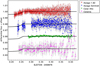 |
Fig. 5 Ground-based photometry collected on the night of 31 January to 01 February 2023 from different European Observatories. |
4 Discussion and conclusions
The main result presented in this work is the detection of a transit in the LC of the young star V1298 Tau collected by CHEOPS between 17 and 18 December 2022. The signal falls within a time interval when a transit of the planet V1298 Tau e was predicted to occur, if its orbital period was, in fact, close to Pe = 45.0033 days. This result does not appear to be compatible with an orbital period close to Pe = 46.7681 days, which is the most probable value proposed by Sikora et al. (2023). This is because no transit would then be expected to fall within the third CHEOPS observing slot, even though this conclusion is necessarily based on a very limited amount of information that we have so far about the orbital dynamics of V1298 Tau e.
We reanalysed the individual transits observed by Kepler/K2 and TESS that have been ascribed to V1298 Tau e and compared them with the signal that we detected in the CHEOPS LC, finding some differences which make a coherent description of this puzzling system challenging. The main observational results and findings from the comparative analysis of the three Kepler/K2, TESS, and CHEOPS transits can be summarised as follows (see Sect. 3.3 for details).
The transit duration as seen by CHEOPS is significantly longer than that derived from Kepler/K2 and TESS observations. We note that our derived transit duration from TESS data is longer than that observed by Kepler/K2, but compatible within ~3σ.
Without constraining the orbital period in the MCMC analysis, we obtained posteriors for Porb that are in agreement within 1σ for the three telescopes, but the impact parameter derived from CHEOPS data is significantly lower
 , as expected for a transit with a longer duration.
The transit depth as seen by CHEOPS is consistent with that of the Kepler/K2 transit, while the transit depth measured from the TESS LC is larger. This implies a radius for the transiting companion of ~0.74 RJup (Kepler/K2 and CHEOPS), or ~0.98 RJup (TESS). We remark that Feinstein et al. (2022) found a radius of ~3σ larger in the TESS data (Rp = 0.89 ± 0.04 RJup) than that found in the Kepler/K2 data by David et al. (2019b); in our case, this discrepancy increases to ~4σ (i.e. the ratio Rp/R★ measured by TESS is ~34% higher than for Kepler/K2). That is because our derived TESS transit is deeper than that of Feinstein et al. (2022), as shown in Fig. 4, implying a larger planet radius (0.98 ± 0.06 vs. 0.89 ± 0.04 RJup).
Regarding the comparison between our derived TESS LC and that of Feinstein et al. (2022), we investigated whether a similar difference in the transit depths is also observed for planet b, which has a transit depth comparable to that of planet e (Appendix B). In this case, we recovered a transit depth slightly shallower, but fully in agreement within the error bars (Fig. B.1). We conclude that it appears that a significant difference with Feinstein et al. (2022) is only observed for planet e.
These results do not have a straightforward interpretation, bringing into question the actual nature of the transiting compan-ion(s). Nonetheless, it must be emphasised that any reasonable explanation is naturally constrained by the limited number of the observed transits. We propose two main interpretative frameworks based on the available data.
First, we begin with the hypothesis that Kepler/K2, TESS, and CHEOPS had indeed observed the same planet V1298 Tau e, as previously identified by David et al. (2019b) and Feinstein et al. (2022). Thanks to CHEOPS, this assumption would solve the uncertainty on the orbital period, implying Pe ~ 45 days, while also implying that the outermost planet in the system experiences changes to the orbital parameters on a timescale of a few years. Indeed, a change in the orbital elements occurring over short timescales would explain the presence of large TTVs (Fig. 6) and transit duration variations (TDV). As an illustrative case, we performed a few N-body numerical integration of the V1298 Tau system for different random choices of the initial orbital angles of planet b and e (mean anomaly and nodal longitude). For this exercise, we adopted the masses of V1298 Tau b and e derived by Suárez Mascareño et al. (2021) and mild eccentricities (0.01–0.05). We see from Fig. C.3 that the orbital period could change significantly over a very short timescale, therefore, the orbit of V1298 Tau e is likely to be chaotic. Changes in the orbital parameters can determine a corresponding change in the transit parameters over a few years, which is an interval similar to the time span covered by the photometric observations. We emphasise that the result of Fig. C.3 is only suggestive because of our limited prior knowledge about the system’s architecture and fundamental properties. As an alternative and illustrative case, we ran another loosely constrained set of dynamical integrations over a time interval of 10 yr by imposing circular orbits and fixing the longitude of the ascending nodes to 180 deg. In this case, planet masses have been drawn from the posteriors derived by Sikora et al. (2023). The results show that there could be a significant probability that we may have missed transits in the first two CHEOPS observing slots, that is if the orbital period Pe is close to 46.76 and 44.17 days, respectively, and TTVs are ≲1 h. If this were the case, it would imply that the observed transit in the third CHEOPS slot belongs to a fifth companion. Any in-depth analysis of the system’s dynamics can be performed only after additional transits of planet e will be observed, and must be left to future studies. We fit the three transits by fixing Pe to 45.0033 days and tested both circular and eccentric orbits (Tables 1 and 2). In all the cases, the BIC statistics does not strongly favour these models over those with Pe treated as a free parameter. The CHEOPS data are better fitted by a circular model (∆BIC = −18), but the posterior of the stellar density significantly differs from the prior. That is not surprising, because a larger stellar radius (lower stellar density) has to be assumed to explain a longer transit duration when fixing Pe to 45 days. We recover a correct stellar density when we include the eccentricity as a free parameter, and we get  . In the cases of Kepler/K2 and TESS, a circular model does not result in a similar issue. This first scenario is tentatively supported by ground-based photometry (Sect. 3.4) that we collected 45 days after the transit detected by CHEOPS. The results from this follow-up do not exclude the possibility that we detected the egress of V1298 Tau e, with the transit occurring approximately −12 h earlier than predicted assuming the reference period from Feinstein et al. (2022). We note that a study of the V1298 Tau system focused on the determination of TTVs is not yet available in the literature. Obviously, to confirm this scenario additional and intensive photometric follow-up is necessary. Unfortunately, at the time of writing, we know that TESS is not going to observe V1298 Tau during Cycle 6 starting from Sept. 20238. New observations with CHEOPS are indeed required and they must be scheduled allowing for a sufficiently large observational window to take into account several hours of TTVs, which are presently not predictable.
Within a second framework, we interpret the transit detected by CHEOPS as due to a new planet-sized companion in the system, different from that observed by Kepler/K2 and TESS, which here we assume to be produced by the same planet. Assuming circular orbits, this would reconcile the different observed transit duration, and it would exclude Pe = 45.0033 days from the list of possible orbital periods of the Kepler/K2 and TESS companion. A future photometric follow-up is indeed necessary also to confirm this scenario, in case no additional transits corresponding to P ~ 45 days will be detected. However, taking into account the 71-day time span of almost uninterrupted observations, the chances that Kepler/K2 would have detected one transit of a planet with Porb = 58 ± 7 days are not negligible, in that it falls nearly 2σ within the duration of the Kepler/K2 observing window.
Whatever the correct scenario is, we need to find an explanation also for the different transit depth observed by Kepler/K2, TESS, and CHEOPS. For a preliminary assessment, we neglect the differences in the Kepler/K2 (CHEOPS) and TESS pass-bands (Fig. 2). In active stars where a significant fraction of the disk is covered by spots, as it is expected in the case of V1298 Tau, unocculted starspots during a transit would produce an apparent increase in the planet’s radius up to 10%, when the transits occur at very different locations in a starspot modulated LC (e.g. see Eq. (17) in Morris 2020). That is to say, assuming that the planet does not cover any of the spots during its transit, when the unocculted spots occupy a smaller area of the stellar disc (i.e. at a maximum of the LC) the out-of-transit stellar brightness baseline will be higher, and the transit depth will be shallower and vice versa. Here, the transits observed by Kepler/K2 and CHEOPS occur close to a minimum in their LCs, while the TESS transit is located close to a maximum of the stellar brightness (Fig. 3). Thus, assuming that the results of a GP model do not depend on where the transit is located on the LC, we would expect the TESS transit to be shallower than the other two, while we observe the opposite. We could reconcile the observations of the three individual transits, at least qualitatively, by assuming that the atmosphere and surface magnetic activity of V1298 Tau is faculae-dominated instead of being spot-dominated. For pre-main sequence stars, this is a plausible scenario, especially for fast rotators for which an anti-correlation between X-ray and simultaneous optical variability is observed (e.g. Guarcello et al. 2019). Nonetheless, that possibility has not been yet investigated for V1298 Tau. We also investigated a possible dependence of the transit depths of planet b from the specific location of the transit signals on the TESS LC. The two transits occurred at different phases of the LC and they perfectly match (Fig. C.4).
Considering the effects of starspot occultation by a transiting planet, this might, in principle, explain the observed differences if we assume an uninterrupted band of dark spots extended in latitude running through all the stellar disk. When the transit chord runs within that band, depending on the fraction of the dark strip covered by the planet disk a transit depth would be more or less affected, and significantly change. This is indeed a ad hoc scenario that should be tested with additional transit observations and modelling, but it would explain the observations if we assume that the planet was covering a larger part of the dark band when observed K2/Kepler and CHEOPS. Starspots on the stellar disc may produce small variations in the apparent duration of a transit (longer or shorter), of the order of 4%, as estimated by Oshagh et al. (2013). Therefore, it looks hard to invoke starspots to explain the 1.5-h longer duration observed by CHEOPS, which is nearly 20% longer than the duration of the Kepler/K2 and TESS transits.
The detection of a new transit-like signal with interesting properties is indeed an important outcome of this study; nonetheless our result does not allow us to draw unambiguous conclusions on the identity of the transiting companion(s) detected by three different telescopes. This outcome is not surprising in that V1298 Tau is a very challenging system to be characterised, both in terms of planet properties and architecture, and stellar activity. The more plausible interpretation may be that we observed the same transiting planet detected by Kepler/K2 and TESS with an orbital period of ~45 days (from a linear ephemeris), which shows TTVs and TDVs due to dynamical instability of its orbit. After all, we detected a transit within the time window where it was expected to occur assuming one of the orbital periods in the grid of Feinstein et al. (2022) as a guidance. The hypothesis of a fifth planet in the system appears less probable with the data currently available. We plan to observe V1298 Tau again with the CHEOPS telescope in the near future, with the primary aim of detecting more transit signals of planet e, and revising the results of this study. The priority will be looking for transits to confirm an orbital period of ~45 days. At the same time, we will analyse a time series of hundreds of RVs of V1298 Tau, most of them collected with the HARPS-N spectrograph as a continuation of the work by Suárez Mascareño et al. (2021). As also shown by the studies of Sikora et al. (2023) and Blunt et al. (2023), the analysis of the RVs for such an active star is notoriously very challenging, especially if the transit ephemeris are not well constrained for all the planets in the system. Our goal will be to exploit the synergy between CHEOPS and RV follow-up in order to improve the characterisation of the orbital and fundamental physical parameters of the planets in the V1298 Tau system. This, in turn, will allow for a well-informed analysis of the planet formation history and of the current architecture and dynamical state of the system, thereby improving the results of a preliminary investigation carried out by Turrini et al. (2023).
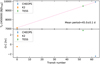 |
Fig. 6 Transit timing variations for the three transits observed by Kepler/K2, TESS, and CHEOPS assuming that they are all ascribable to V1298 Tau e. The observed epochs of central transit have been fitted with a linear function, resulting in a mean orbital period of 45.0 ± 0.1 days. |
Acknowledgements
This work has been supported by the PRIN-INAF 2019 “Planetary systems at young ages (PLATEA)” and ASI-INAF agreement n.2018- 16-HH.0. CHEOPS is an ESA mission in partnership with Switzerland with important contributions to the payload and the ground segment from Austria, Belgium, France, Germany, Hungary, Italy, Portugal, Spain, Sweden and the United Kingdom. G.S., V.N., G.B., and L.B. acknowledge support from CHEOPS ASI-INAF agreement n. 2019-29-HH.0. L.M. acknowledges support from the “Fondi di Ricerca Scientifica d’Ateneo 2021” of the University of Rome “Tor Vergata”. A.S.M. acknowledges financial support from the Spanish MICINN project PID2020-117493GB-I00 and the Government of the Canary Islands project ProID2020010129. V.B., M.M., N.L., and M.Z. acknowledge support from the Agencia Estatal de Investigación del Ministerio de Ciencia e Innovación under grants PID2019-109522GBC51(53). This work includes data collected with the TESS mission, obtained from the MAST data archive at the Space Telescope Science Institute (STScI). Funding for the TESS mission is provided by the NASA Explorer Program. STScI is operated by the Association of Universities for Research in Astronomy, Inc., under NASA contract NAS 5–26555. This paper also includes data collected by the Kepler mission and obtained from the MAST data archive at the Space Telescope Science Institute (STScI). Funding for the Kepler mission is provided by the NASA Science Mission Directorate. STScI is operated by the Association of Universities for Research in Astronomy, Inc., under NASA contract NAS 5–26555. The results presented in this work are also based on observations collected at the Centro Astronómico Hispano en Andalucía (CAHA) at Calar Alto, operated jointly by Junta de Andalucía and Consejo Superior de Investigaciones Científicas (IAA- CSIC), and at Copernico 1.82 m and Schmidt 67/92 telescopes (Asiago Mount Ekar, Italy), INAF – Osservatorio Astronomico di Padova. We kindly thank S. Ciroi for having shared his observing time at the Copernico 1.82 m telescope. This work is dedicated to the memory of A.C.P., a young star returned too soon among the stars.
Appendix A GP modelling of the light curves
The Kepler/K2 and TESS LCs of V1298 Tau clearly show a periodic signal that gradually changes with time. This kind of correlated noise is typically generated by stellar active regions co-rotating with the star. To extract the characteristic frequencies of the stellar signal, we first masked the planetary transits in the Kepler/K2 and TESS LCs by using the ephemeris obtained by David et al. (2019b) and Feinstein et al. (2022). Then we computed the power spectral density (PSD) of the remaining LCs using LS periodogram (Scargle 1982). Both periodograms show two peaks at frequencies v ~ 0.35 d−1 and v ~ 0.70 d−1 respectively (Fig. A.1). Since the latter is twice the former, we speculate that the peak at lower frequency corresponds to the stellar rotation (Prot ~2.9 d), while the second peak is its first harmonic.
In their analysis of the planetary transits, David et al. (2019b) and Feinstein et al. (2022) modelled the stellar variability as a “rotation” GP defined as the sum of two simple harmonic oscillator (SHO) kernels. The simple SHO kernel takes a PSD of the form:
 (A.1)
(A.1)
where v0 is the undamped frequency of the oscillator (not to confuse with the corresponding angular frequency ω0), S0 fixes the scale of the PSD and Q is the quality factor of the oscillations. The simple SHO kernel can model only one peak in the PSD of the data. In the case of pluri-modal PSDs, a SHO for each mode in the PSD is needed. This explains the approach of David et al. (2019b) and Feinstein et al. (2022).
The exact parametrisation of the mixture of SHO kernels is discussed in David et al. (2019b). Since it is difficult to relate the mathematical representation of this GP (scale S and quality Q) to the physical properties of the LCs (amplitude of the correlated noise and its timescale), we converted the best-fit GP parameters into physical via the following equations9:
 (A.2)
(A.2)
 (A.3)
(A.3)
 (A.4)
(A.4)
For the case of the Kepler/K2 LC, David et al. (2019b) derived two SHO GPs with periods of 2.87 d and 5.74 d, amplitudes of 12 mmag and 7 mmag and timescales of 14 d and 5 d. For the TESS LC, Feinstein et al. (2022) used the same rotation GP model and they obtained periods of 2.97 d and 5.94 d and timescales of 6 d and 1 d. Unfortunately, they forgot to report the scales S of the two GPs, which are needed to compute the corresponding noise amplitudes. In the following discussion, we thus assume the same amplitudes derived by David et al. (2019b).
In both cases, the stellar rotation period is successfully recovered as the periodicity of the first SHO component, the second component corresponding to the first harmonic. We remark though that the timescales of the rotation GP are a few times the period of the oscillations (2.87 d and 2.97 d for Kepler/K2 and TESS respectively). This is critical in particular for the TESS analysis, where the first SHO component has a timescale of roughly two oscillation periods, while the second component has a timescale that comparable with or shorter than the stellar rotation period. From a physical point of view, when the timescale of the oscillation is close or less than the period of the oscillations, then the periodicity of the signal is suppressed by the fast exponential decay due to the short timescale. As a result, such systems do show a correlated signal but without the characteristic repeating pattern similar to undamped oscillators, clearly visible in the Kepler/K2 and TESS LCs (Fig. 3).
From a more quantitative perspective, we compared the PSD of the data with the typical PSD corresponding to the GPs derived by David et al. (2019b) and Feinstein et al. (2022). For each GP, we generated 1000 LCs using the same timestamps of the corresponding LC (either Kepler/K2 or TESS) to take into account any aliasing effect due to the time sampling. Finally, for each set of 1000 LSs, we computed the average LS periodogram and its 1- σ uncertainty. The results are shown in Fig. A.1. The most striking feature of these average periodograms is that they recover the two peaks in the periodogram of the data, but the peaks are broader than the peaks in the periodogram of the data. This means that the quality factor Q of the oscillations in the rotation GPs underestimate the true values or, in physical units, the timescales of the oscillations are shorter than in the data. This is most critical for the TESS LC, where the Q of the second SHO GP is so low (and the corresponding timescale is so short) that the corresponding peak at v ~ 0.70 d−1 is completely flattened out.
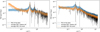 |
Fig. A.1 Analysis of the PSD of the Kepler/K2 (left) and TESS (right) LCs. In each panel, the black solid line shows the PSD of the LC after masking the planetary transits. The two vertical dashed lines mark the frequencies 0.35 d−1 and 0.70 d−1. The confidence band in orange shows the average periodogram obtained using the rotation GP, as discussed in the text. Similarly, the blue confidence band corresponds to the GP model used in this work. |
A closer look at the periodograms shows a hint of a decreasing slope at low frequencies (v < 0.3 d−1). This may indicate the presence of an additional correlated noise (other than the stellar rotation) with a PSD that decreases with v. The presence of a slope at low frequencies is a challenge for the SHO GP and also for the rotation GP, as by construction their corresponding PSD is flat for frequencies lower than the peak frequencies.
We ran a few simulation tests by generating LCs using a rotation GP combined with an overdamped SHO, whose PSD monotonically decreases with v (Foreman-Mackey et al. 2017). In order to save computing time, we fitted the LCs by means of least-square regression. We found that the presence of a neglected GP biases the fit of the rotation GP towards lower quality factors and shorter timescales. In the most critical cases, the fit of the rotation GP also diverged towards unrealistic timescales and/or amplitudes of the correlated noise. This can explain why David et al. (2019b) and Feinstein et al. (2022) use informative priors in their analysis. In the frequency domain, the fit of the simulated LCs leads to a rotation GP whose corresponding LS periodogram has broader peaks compared to the periodogram of the fitted LC. In other words, the best-fit rotation GP tries to include the spectral power due to the extra GP by broadening the rotation peaks.
In the domain of Fourier analysis, the assumption of a PSD that does not match the observations leads to a biased spectral decomposition of the signal. It is difficult to asses how this translates in the GP analysis framework and any further detailed analysis is not the scope of this work. Nonetheless, we tested a different GP for two reasons. First of all, we aimed at a better representation of the correlated noise in the Kepler/K2 and TESS LCs in order to put our analysis on more solid ground. Secondly, we wanted to asses how the planetary parameters are affected by the choice of a different GP model.
We modelled the correlated noise using the S+LEAF python library (version 2.1.2 Delisle et al. 2020, 2022). This library implements the exponential-sine periodic (ESP) GP, an approximation of the quasi-periodic kernel, with the generic element of the kernel matrix k(∆t) described by the equation:
 (A.5)
(A.5)
where σESP is the standard deviation of the GP, λESP is its timescale, vESP is the rotational frequency (≡ vrot in Table 1), and ηESP is the scale of the oscillations, which sets how the spectral power is distributed among the harmonics of the periodic signal. In the current implementation of this kernel it is necessary to set the number of harmonics to include through the nharm keyword: since the PSD of the data shows two predominant peaks (the fundamental and first harmonics), we manually set the nharm = 2.
We initially tried to use this GP to fit by least-square regression the same stellar LCs discussed above, but we did not find any satisfactory results, mainly because the fit did not converge to a realistic set of GP parameters. Once again, some tests showed that a low-frequency power excess might prevent the ESP GP to properly model the correlated noise on its own. We thus added an extra SHO GP in order to take into account the slope at low frequencies discussed above, obtaining a more meaningful set of GP parameters.
First of all, for the Kepler/K2 LC the ESP GP converged to  and λESP=17 d, while for the TESS LC we obtained σESP = 11 mmag, PESP=2.90 d and λESP = 30 d. Thus, we recovered similar periodicities, timescales and amplitudes for the two LCs, small differences being likely due to differences in the bandpasses and/or different active stellar latitudes at the epoch of the observations. Most importantly, we derived a GP timescale approximately an order of magnitude longer than the rotation period.
The SHO GP converged to σSHO=1.7 (3.3) ppm, ¶SHO=1 (2) d and λSHO=0.4 (0.2) d for the Kepler/K2 (TESS) LC. By means of Eqs. A.2–A.3, these parameters translate into Q=1.2 and Q=0.3 for the Kepler/K2 and TESS LC respectively. These two quality factors are close to the critical damping value of  , below which the PSD of the SHO GP becomes monotonically decreasing with v. From a physical point of view, this corresponds to an overdamped GP that can be representative of low-frequencies stellar processes. As an example, the overdamped SHO GP with fixed Q = 1/2 is commonly used to model the surface granulation of convective stars (Harvey 1985; Kallinger et al. 2014).
Similarly to what we have done above, we used our best-fit composite GP to simulate 1000 LCs, using either the time sampling of Kepler/K2 or TESS. Then we computed the mean LS periodogram, obtaining the PSDs shown in Fig. A.1. Our GP model is able to better reproduce the two peaks in the PSD of the data and also provides a better match at low frequencies. For all the reasons discussed so far in this Appendix, in our combined analysis of the stellar correlated signal and the planetary transits (Sect. 3.1 and 3.2) we adopted the mixture of a SHO and a ESP GP models. We also remark that we used uninformative priors on all the GP parameters (see Table 1) without any issue in the convergence of the MCMC chains.
Appendix B Comparing our TESS transit of V1298 Tau b with the analysis of Feinstein et al. (2022)
To assess whether and how our pipeline to extract the TESS LC (Sect. 2.2) and GP model affect the properties of the transits with respect to the analysis of Feinstein et al. (2022), we also considered transits of planet b. To simplify the analysis, we only focused on the transit around BJD 2457 091.2 in the Kepler/K2 LC, and the transit around BJD 2459 505.2 in the TESS LC. These transits do not overlap with transits of other planets, and are well sampled. The results of our LC fitting are shown in Fig. B.1, together with the best-fit rotational GP signal derived by David et al. (2019b) and Feinstein et al. (2022). Our derived depth for the TESS transit is  , which is shallower than the transit analysed by Feinstein et al. (2022)
  , with a discrepancy
  . We confirm the difference in the transit depth as seen by the Kepler/K2 and TESS telescopes pointed out by Feinstein et al. (2022).
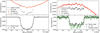 |
Fig. B.1 Portions of Kepler/K2 and TESS LCs showing a transit of planet V1298 Tau b (left and right panel respectively). The plots at the top show the undetrended LCs analysed in our work centred on the transit (black dots), and the data after removing the best-fit planetary transit (red dots) to show the GP signal during the transit timespan. The plots at the bottom show the transit signals after subtracting the best-fit GP model. The corresponding detrended and flattened TESS light curve analysed by Feinstein et al. (2022) is shown for comparison (green cross symbols). It has been obtained from the jupyter notebook made publicly available by Feinstein et al. (2022)10. |
Appendix C Additional plots
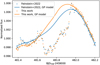 |
Fig. C.1 Comparison between our extracted TESS LC (orange dots) showing the transit attributed to V1298 Tau e, and the one extracted by Feinstein et al. (2022) (blue dots), including the corresponding best-fit GP models (solid curves). |
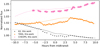 |
Fig. C.2 Undetrended LCs of the three transits analysed in our work and shown in Fig. 4 (Kepler/K2, TESS, and CHEOPS), with our calculated best-fit GP models overplotted. An offset has been added to each curve in order to improve the clarity of the plot. |
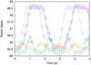 |
Fig. C.3 Temporal evolution of the orbital period of V1298 Tau e, assuming that K2/Kepler, TESS, and CHEOPS observed a transit of the same planet. This illustrative result is based on a few simulated N- body integrations covering a time span of five years, as described in Section 4. Each curve in the plot represents a simulation. |
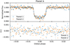 |
Fig. C.4 Comparison between the two consecutive transits of V1298 Tau b observed by TESS around epochs BJDTDB 2 459 481 (transit 1) and 2 459 505 (transit 2). |
References
- Benz, W., Broeg, C., Fortier, A., et al. 2021, Exp. Astron., 51, 109 [Google Scholar]
- Bertocco, S., Goz, D., Tornatore, L., et al. 2020, ASP Conf. Ser., 527, 303 [NASA ADS] [Google Scholar]
- Blunt, S., Carvalho, A., David, T. J., et al. 2023, AJ, 166, 62 [NASA ADS] [CrossRef] [Google Scholar]
- Brandeker, A., Heng, K., Lendl, M., et al. 2022, A&A, 659, L4 [NASA ADS] [CrossRef] [EDP Sciences] [Google Scholar]
- Collins, K. A., Kielkopf, J. F., Stassun, K. G., & Hessman, F. V. 2017, AJ, 153, 77 [Google Scholar]
- David, T. J., Cody, A. M., Hedges, C. L., et al. 2019a, AJ, 158, 79 [NASA ADS] [CrossRef] [Google Scholar]
- David, T. J., Petigura, E. A., Luger, R., et al. 2019b, ApJ, 885, L12 [Google Scholar]
- Delisle, J. B., Hara, N., & Ségransan, D. 2020, A&A, 638, A95 [EDP Sciences] [Google Scholar]
- Delisle, J. B., Unger, N., Hara, N. C., & Ségransan, D. 2022, A&A, 659, A182 [NASA ADS] [CrossRef] [EDP Sciences] [Google Scholar]
- Feinstein, A. D., Montet, B. T., Johnson, M. C., et al. 2021, AJ, 162, 213 [NASA ADS] [CrossRef] [Google Scholar]
- Feinstein, A. D., David, T. J., Montet, B. T., et al. 2022, ApJ, 925, L2 [NASA ADS] [CrossRef] [Google Scholar]
- Foreman-Mackey, D., Hogg, D. W., Lang, D., & Goodman, J. 2013, PASP, 125, 306 [Google Scholar]
- Foreman-Mackey, D., Agol, E., Ambikasaran, S., & Angus, R. 2017, AJ, 154, 220 [Google Scholar]
- Gaidos, E., Hirano, T., Beichman, C., et al. 2022, MNRAS, 509, 2969 [Google Scholar]
- Goodman, J., & Weare, J. 2010, Commun. Appl. Math. Comput. Sci., 5, 65 [Google Scholar]
- Guarcello, M. G., Flaccomio, E., Micela, G., et al. 2019, A&A, 628, A74 [NASA ADS] [CrossRef] [EDP Sciences] [Google Scholar]
- Harvey, J. 1985, ESA Spec. Publ., 235, 199 [Google Scholar]
- Hoyer, S., Guterman, P., Demangeon, O., et al. 2020, A&A, 635, A24 [NASA ADS] [CrossRef] [EDP Sciences] [Google Scholar]
- Johnson, M. C., David, T. J., Petigura, E. A., et al. 2022, AJ, 163, 247 [NASA ADS] [CrossRef] [Google Scholar]
- Kallinger, T., De Ridder, J., Hekker, S., et al. 2014, A&A, 570, A41 [NASA ADS] [CrossRef] [EDP Sciences] [Google Scholar]
- Kipping, D. M. 2010, MNRAS, 408, 1758 [Google Scholar]
- Landsman, W. B. 1993, ASP Conf. Ser., 52, 246 [Google Scholar]
- Luger, R., Kruse, E., Foreman-Mackey, D., Agol, E., & Saunders, N. 2018, AJ, 156, 99 [Google Scholar]
- Maggio, A., Locci, D., Pillitteri, I., et al. 2022, ApJ, 925, 172 [NASA ADS] [CrossRef] [Google Scholar]
- Malavolta, L., Nascimbeni, V., Piotto, G., et al. 2016, A&A, 588, A118 [NASA ADS] [CrossRef] [EDP Sciences] [Google Scholar]
- Malavolta, L., Mayo, A. W., Louden, T., et al. 2018, AJ, 155, 107 [NASA ADS] [CrossRef] [Google Scholar]
- Morris, B. M. 2020, ApJ, 893, 67 [Google Scholar]
- Nardiello, D., Bedin, L. R., Nascimbeni, V., et al. 2015, MNRAS, 447, 3536 [CrossRef] [Google Scholar]
- Nardiello, D., Libralato, M., Bedin, L. R., et al. 2016, MNRAS, 455, 2337 [NASA ADS] [CrossRef] [Google Scholar]
- Nardiello, D., Borsato, L., Piotto, G., et al. 2019, MNRAS, 490, 3806 [NASA ADS] [CrossRef] [Google Scholar]
- Nardiello, D., Piotto, G., Deleuil, M., et al. 2020, MNRAS, 495, 4924 [Google Scholar]
- Nardiello, D., Deleuil, M., Mantovan, G., et al. 2021, MNRAS, 505, 3767 [NASA ADS] [CrossRef] [Google Scholar]
- Nardiello, D., Malavolta, L., Desidera, S., et al. 2022, A&A, 664, A163 [NASA ADS] [CrossRef] [EDP Sciences] [Google Scholar]
- Nascimbeni, V., Piotto, G., Bedin, L. R., & Damasso, M. 2011, A&A, 527, A85 [NASA ADS] [CrossRef] [EDP Sciences] [Google Scholar]
- Nascimbeni, V., Cunial, A., Murabito, S., et al. 2013, A&A, 549, A30 [NASA ADS] [CrossRef] [EDP Sciences] [Google Scholar]
- Oshagh, M., Santos, N. C., Boisse, I., et al. 2013, A&A, 556, A19 [NASA ADS] [CrossRef] [EDP Sciences] [Google Scholar]
- Parviainen, H., & Korth, J. 2020, MNRAS, 499, 3356 [NASA ADS] [CrossRef] [Google Scholar]
- Poppenhaeger, K., Ketzer, L., & Mallonn, M. 2021, MNRAS, 500, 4560 [Google Scholar]
- Scandariato, G., Singh, V., Kitzmann, D., et al. 2022, A&A, 668, A17 [NASA ADS] [CrossRef] [EDP Sciences] [Google Scholar]
- Scargle, J. D. 1982, ApJ, 263, 835 [Google Scholar]
- Sikora, J., Rowe, J., Barat, S., et al. 2023, AJ, 165, 250 [NASA ADS] [CrossRef] [Google Scholar]
- Sokal, A. 1997, Monte Carlo Methods in Statistical Mechanics: Foundations and New Algorithms, eds. C. DeWitt-Morette, P. Cartier, & A. Folacci (Boston, MA: Springer US), 131 [Google Scholar]
- Southworth, J., Hinse, T. C., Jørgensen, U. G., et al. 2009, MNRAS, 396, 1023 [NASA ADS] [CrossRef] [Google Scholar]
- Suárez Mascareño, A., Damasso, M., Lodieu, N., et al. 2021, Nat. Astron., 6, 232 [Google Scholar]
- Taffoni, G., Becciani, U., Garilli, B., et al. 2020, ASP Conf. Ser., 527, 307 [NASA ADS] [Google Scholar]
- Tejada Arevalo, R., Tamayo, D., & Cranmer, M. 2022, ApJ, 932, L12 [NASA ADS] [CrossRef] [Google Scholar]
- Turrini, D., Marzari, F., Polychroni, D., et al. 2023, A&A, 679, A55 [NASA ADS] [CrossRef] [EDP Sciences] [Google Scholar]
- Vissapragada, S., Stefánsson, G., Greklek-McKeon, M., et al. 2021, AJ, 162, 222 [NASA ADS] [CrossRef] [Google Scholar]
We based our proposal on the hypothesis by Feinstein et al. (2022) that the two individual transits observed by Kepler/K2 and TESS belong to the same planetary companion V1298 Tau e.
Feinstein et al. (2022) found  using their version of TESS photometry, corresponding to a transit depth 0.0043 ± 0.0003.
All Tables
All Figures
|
Fig. 1 Light curve of V1298 Tau collected on the night of 8 February 2022 with the Schmidt 67/92 cm telescope at the INAF-Astrophysical Observatory of Asiago. The red dots correspond to the binned light curve, and the green curve represents the transit model of planet e based on the ephemeris and transit depth derived by Feinstein et al. (2022). |
| In the text | |
|
Fig. 2 Bandpasses of Kepler/K2, TESS, and CHEOPS normalised to their peak values, as a function of wavelength. The cyan and red curves represent the spectral energy distributions of a Teff = 5500 K and Teff = 4500 K dwarf star, respectively (image taken from https://www.cosmos.esa.int/web/cheops/performances-bandpass). |
| In the text | |
|
Fig. 3 Kepler/K2, TESS, and CHEOPS LCs of V 1298 Tau from top to bottom row, respectively. In each panel, the blue solid line shows the best-fit model. The arrows indicate the transits of the companion labelled as planet e by David et al. (2019b) and Feinstein et al. (2022), based on data from K2 and TESS. |
| In the text | |
|
Fig. 4 Comparison of the detrended transit LCs discussed in this work as seen by Kepler/K2, TESS and CHEOPS. For each dataset, the best-fit transit model is shown by curves with the same colour as the data points. The green data points identify the detrended and flattened TESS light curve analysed by Feinstein et al. (2022), obtained from the jupyter notebook made publicly available by the authors online (https://github.com/afeinstein20/v1298tau_tess/blob/main/notebooks/TESS_V1298Tau.ipynb). |
| In the text | |
|
Fig. 5 Ground-based photometry collected on the night of 31 January to 01 February 2023 from different European Observatories. |
| In the text | |
|
Fig. 6 Transit timing variations for the three transits observed by Kepler/K2, TESS, and CHEOPS assuming that they are all ascribable to V1298 Tau e. The observed epochs of central transit have been fitted with a linear function, resulting in a mean orbital period of 45.0 ± 0.1 days. |
| In the text | |
|
Fig. A.1 Analysis of the PSD of the Kepler/K2 (left) and TESS (right) LCs. In each panel, the black solid line shows the PSD of the LC after masking the planetary transits. The two vertical dashed lines mark the frequencies 0.35 d−1 and 0.70 d−1. The confidence band in orange shows the average periodogram obtained using the rotation GP, as discussed in the text. Similarly, the blue confidence band corresponds to the GP model used in this work. |
| In the text | |
|
Fig. B.1 Portions of Kepler/K2 and TESS LCs showing a transit of planet V1298 Tau b (left and right panel respectively). The plots at the top show the undetrended LCs analysed in our work centred on the transit (black dots), and the data after removing the best-fit planetary transit (red dots) to show the GP signal during the transit timespan. The plots at the bottom show the transit signals after subtracting the best-fit GP model. The corresponding detrended and flattened TESS light curve analysed by Feinstein et al. (2022) is shown for comparison (green cross symbols). It has been obtained from the jupyter notebook made publicly available by Feinstein et al. (2022)10. |
| In the text | |
|
Fig. C.1 Comparison between our extracted TESS LC (orange dots) showing the transit attributed to V1298 Tau e, and the one extracted by Feinstein et al. (2022) (blue dots), including the corresponding best-fit GP models (solid curves). |
| In the text | |
|
Fig. C.2 Undetrended LCs of the three transits analysed in our work and shown in Fig. 4 (Kepler/K2, TESS, and CHEOPS), with our calculated best-fit GP models overplotted. An offset has been added to each curve in order to improve the clarity of the plot. |
| In the text | |
|
Fig. C.3 Temporal evolution of the orbital period of V1298 Tau e, assuming that K2/Kepler, TESS, and CHEOPS observed a transit of the same planet. This illustrative result is based on a few simulated N- body integrations covering a time span of five years, as described in Section 4. Each curve in the plot represents a simulation. |
| In the text | |
|
Fig. C.4 Comparison between the two consecutive transits of V1298 Tau b observed by TESS around epochs BJDTDB 2 459 481 (transit 1) and 2 459 505 (transit 2). |
| In the text | |
Current usage metrics show cumulative count of Article Views (full-text article views including HTML views, PDF and ePub downloads, according to the available data) and Abstracts Views on Vision4Press platform.
Data correspond to usage on the plateform after 2015. The current usage metrics is available 48-96 hours after online publication and is updated daily on week days.
Initial download of the metrics may take a while.